
Spatiotemporal Characteristics and Determinants of Rural Construction Land in China’s Developed Areas: A Case Study of the Yangtze River Delta
Abstract
:1. Introduction
2. Study Area and Methodology
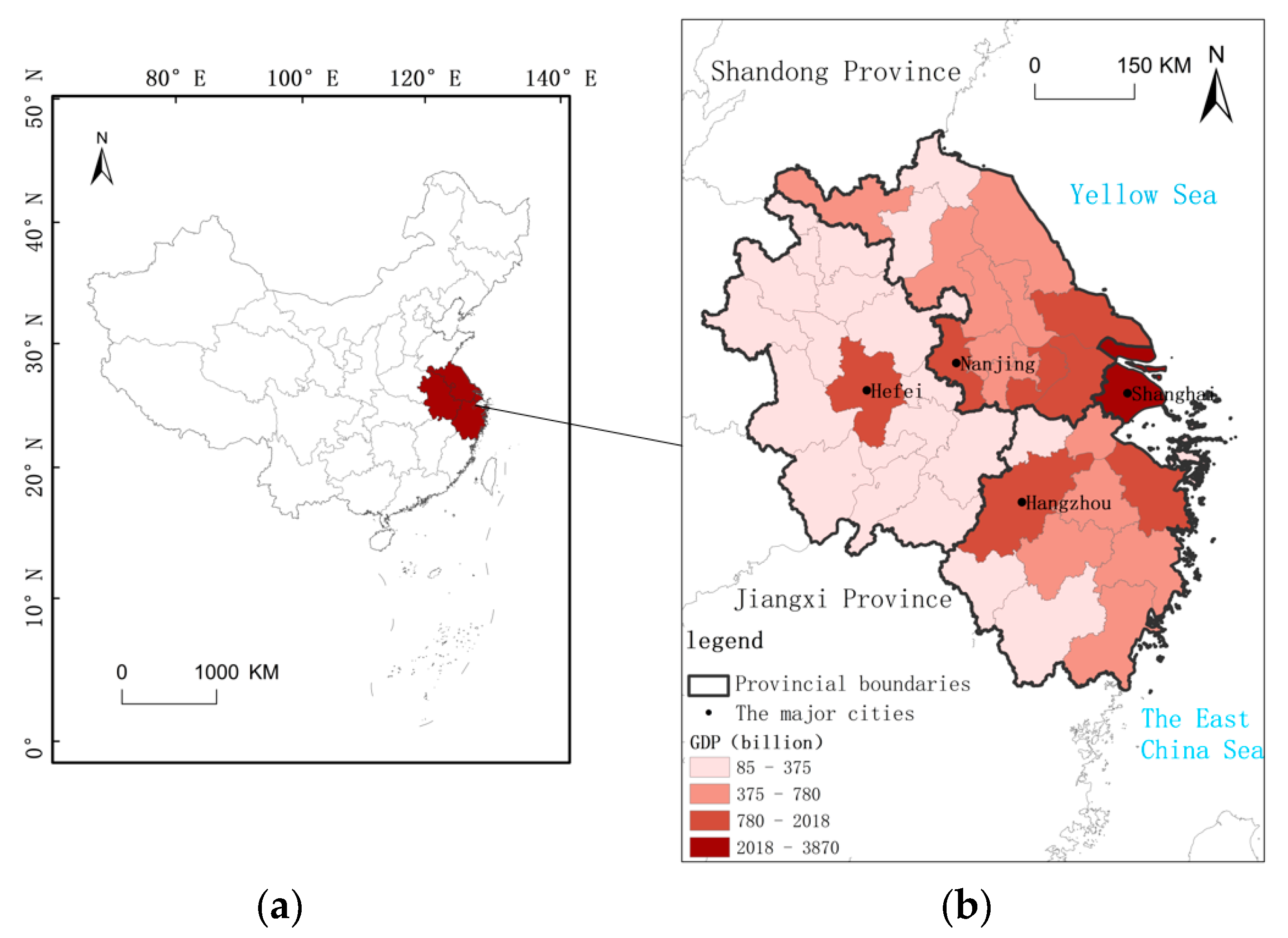
2.1. Study Area
2.2. Data
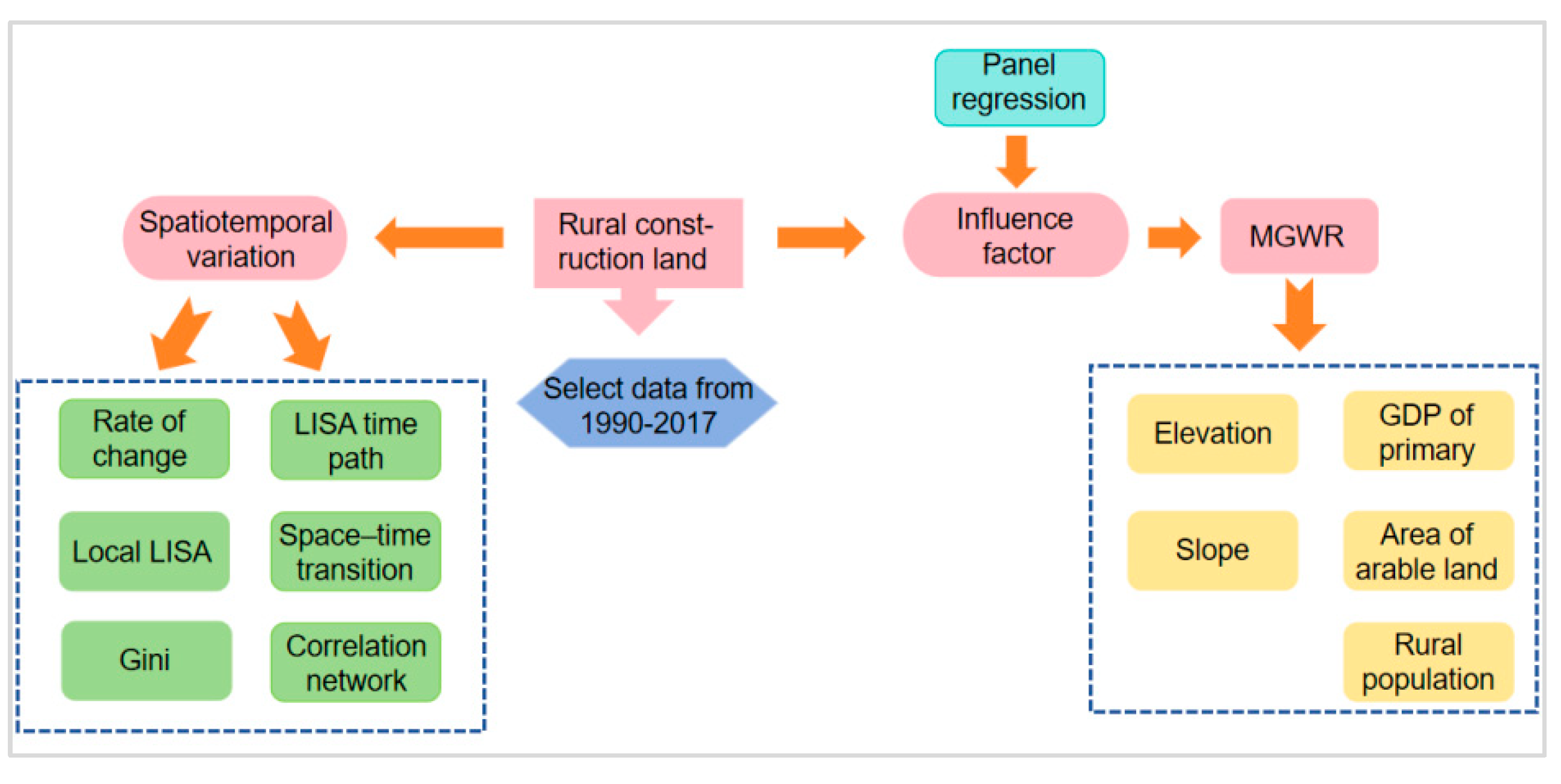
2.3. Methodology
2.3.1. Annual Growth Rate of Construction Land
2.3.2. Gini Coefficient
2.3.3. Exploratory Spatiotemporal Data Analysis (ESTDA)
- (1)
- Moran’s I
- (2)
- LISA (Local Indicators of Spatial Association) time path
- (3)
- LISA space–time transition
- (4)
- Correlation network
2.3.4. Multiscale Geographically Weighted Regression (MGWR)
3. Results
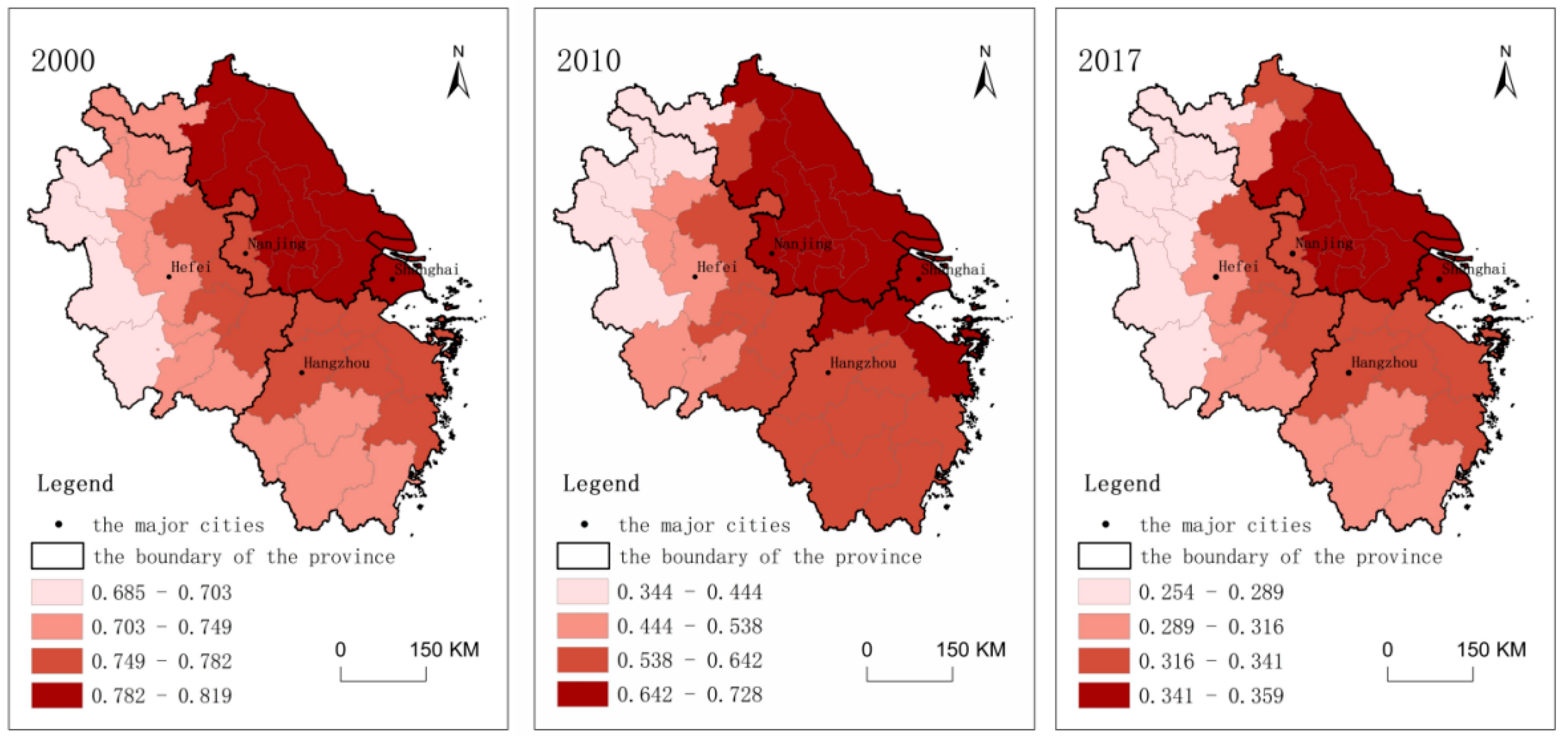
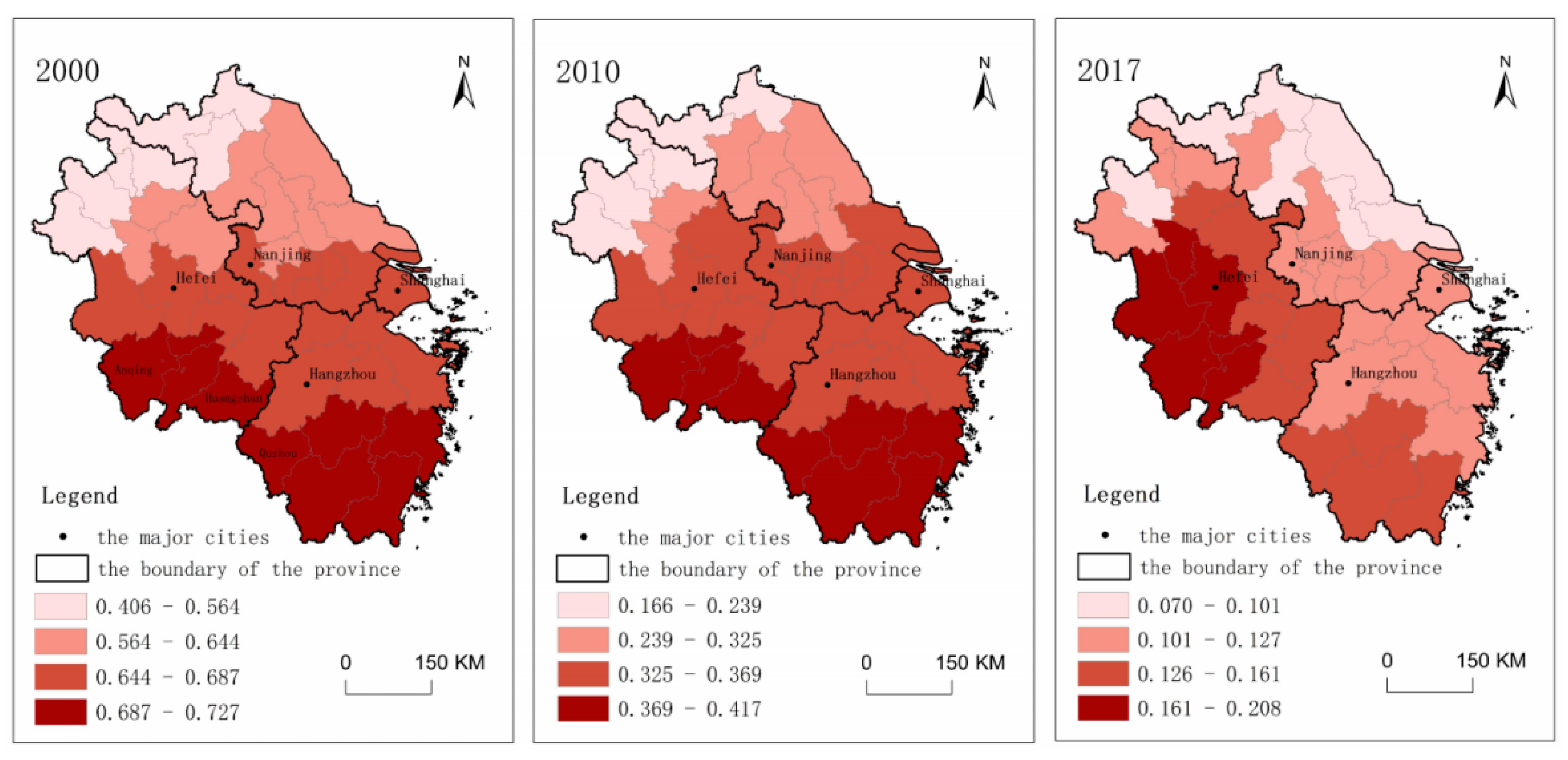
3.1. Spatiotemporal Dynamics of RCL in the YRD Region
3.1.1. Spatial and Temporal Patterns of RCL in the YRD Region
- (1)
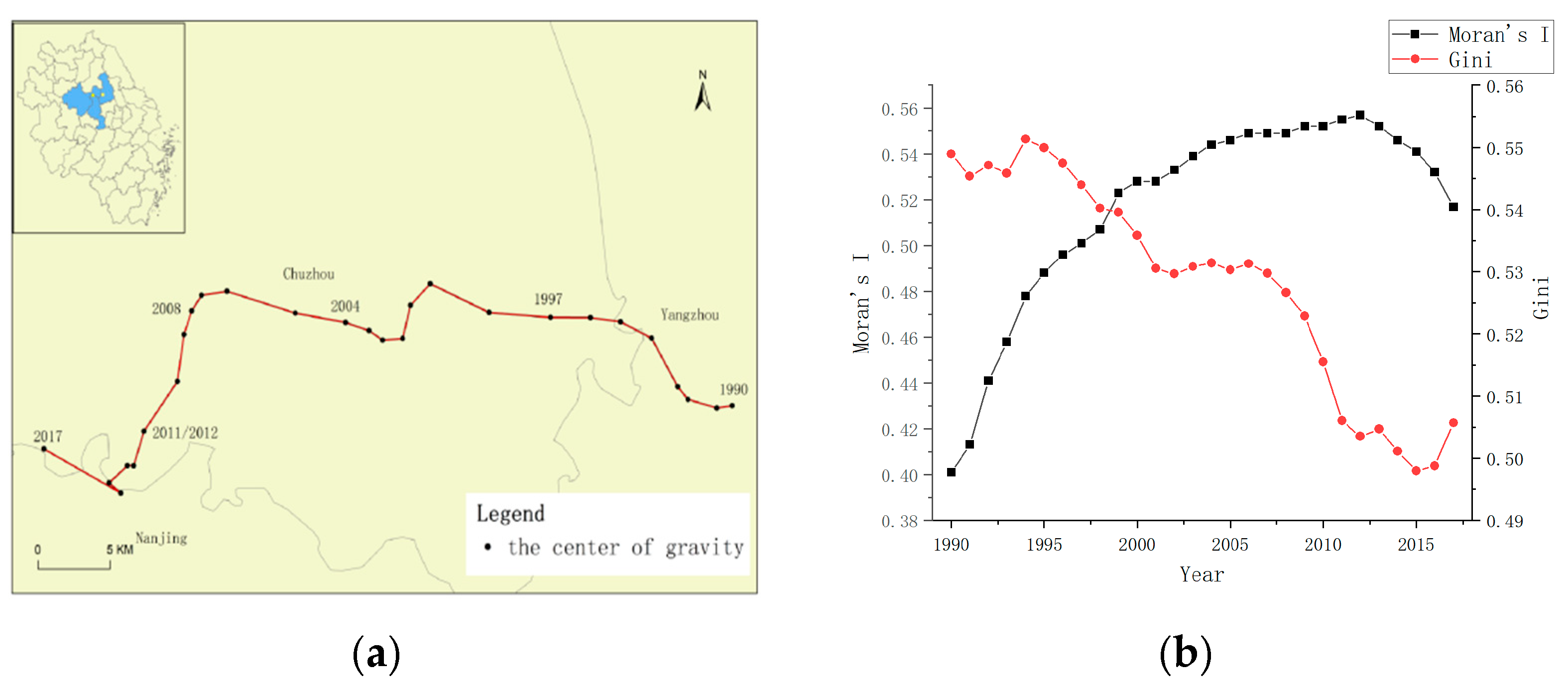
- Global features
- (2)
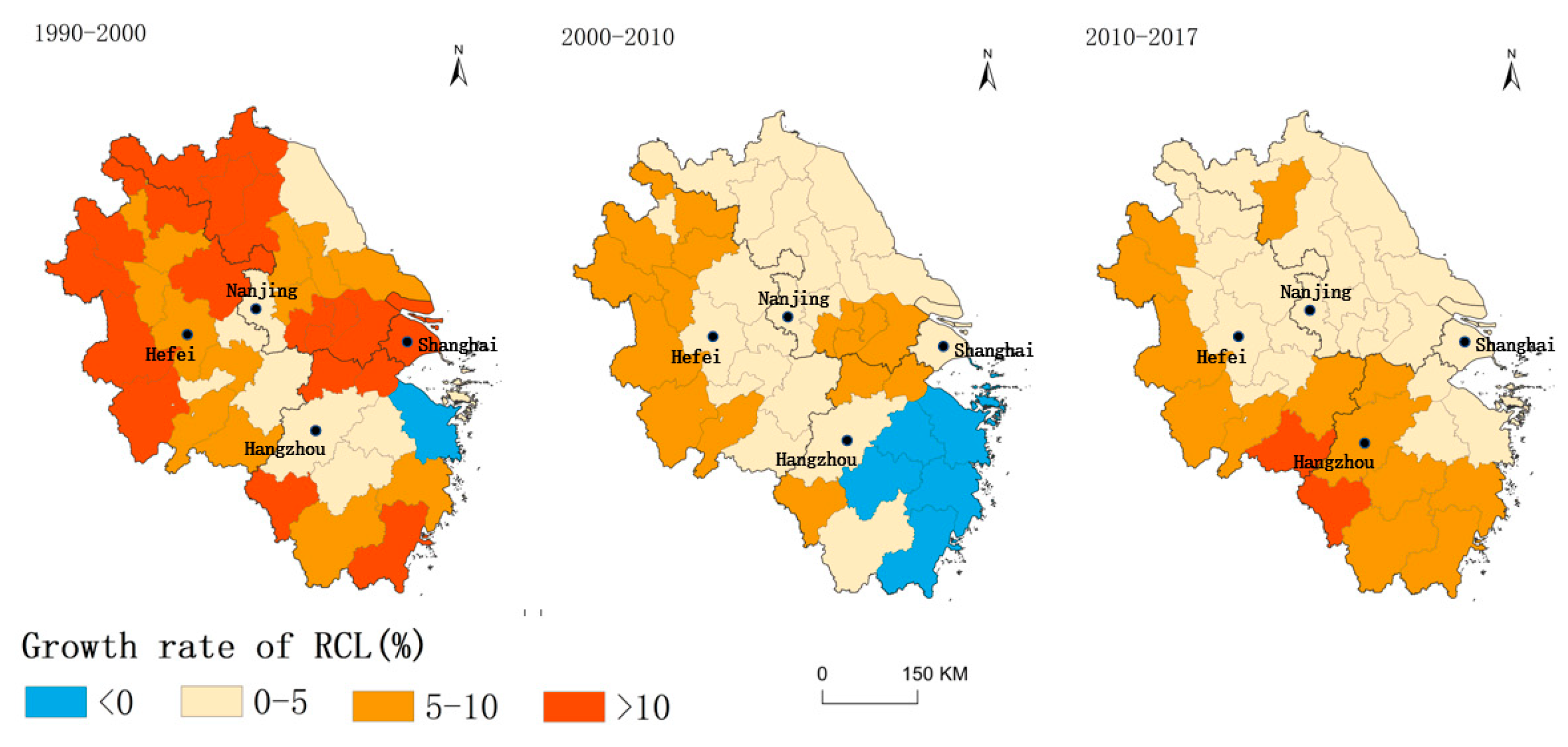
- Spatial and temporal patterns of changes in RCL
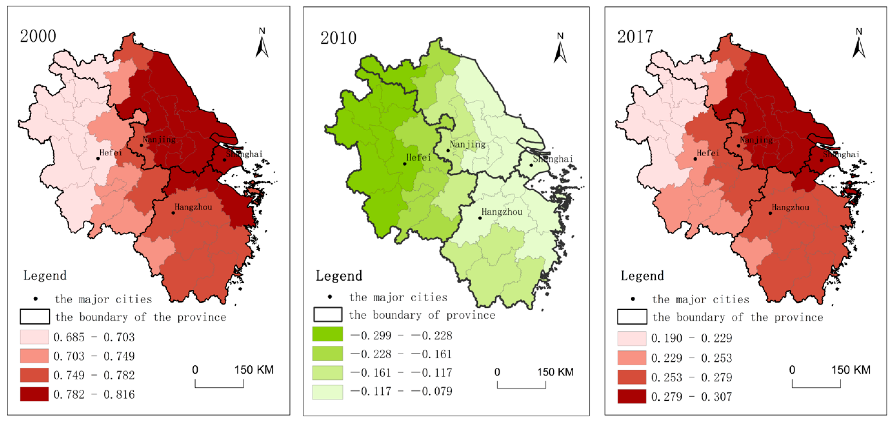
3.1.2. Dynamics of the Local Spatial Dependence of RCL
3.1.3. Local Clustering of Changes in RCL
3.1.4. Inter-City Competition for RCL
3.2. Determinants of RCL
3.2.1. Baseline Results
3.2.2. Spatial and Temporal Variations in the Effects of the Determinants
- (1)
- GDP of primary industry
- (2)
- Area of arable land
- (3)
- Elevation and slope
- (4)
- Rural population
4. Discussion
4.1. Mechanisms of the Effects of Determinants on RCL
4.2. Other Factors Influencing RCL
4.3. Policy Implications
4.4. Contributions and Limitations
5. Conclusions
Author Contributions
Funding
Data Availability Statement
Acknowledgments
Conflicts of Interest
References
- The Impact of Global Land-Cover Change on the Terrestrial Water Cycle|Nature Climate Change. Available online: https://www.nature.com/articles/nclimate1690 (accessed on 16 August 2023).
- Liao, G.; He, P.; Gao, X.; Lin, Z.; Huang, C.; Zhou, W.; Deng, O.; Xu, C.; Deng, L. Land use optimization of rural production–living–ecological space at different scales based on the BP–ANN and CLUE–S models. Eco. Ind 2022, 137, 108710. [Google Scholar] [CrossRef]
- Qu, Y.; Zhan, L.; Jiang, G.; Ma, W.; Dong, X. How to Address “Population Decline and Land Expansion (PDLE)” of Rural Residential Areas in the Process of Urbanization: A Comparative Regional Analysis of Human-Land Interaction in Shandong Province. Habitat Int. 2021, 117, 102441. [Google Scholar] [CrossRef]
- Liu, Y.; Yang, R.; Long, H.; Gao, J.; Wang, J. Implications of Land-Use Change in Rural China: A Case Study of Yucheng, Shandong Province. Land Use Policy 2014, 40, 111–118. [Google Scholar] [CrossRef]
- Long, H.; Li, Y.; Liu, Y.; Woods, M.; Jian, Z. Accelerated Restructuring in Rural China Fueled by “increasing vs. Decreasing Balance” Land-Use Policy for Dealing with Hollowed Villages. Land Use Policy 2012, 29, 11–22. [Google Scholar] [CrossRef]
- Juan, R. Cuadrado-Roura Population Imbalances in Europe. Urban Concentration versus Rural Depopulation. Reg. Sci. Policy Pract. 2023, 15, 713–716. [Google Scholar]
- Deng, X.; Yuan, Y.; Li, Z.; Song, W.; W, Z. Impacts of Land-Use Change on Valued Ecosystem Service in Rapidly Urbanized North China Plain. Ecol. Mod. 2015, 318, 245–253. [Google Scholar] [CrossRef]
- Alexandratos, N. Countries with Rapid Population Growth and Resource Constraints: Issues of Food, Agriculture, and Development. Popul. Dev. Rev. 2005, 31, 237–258. [Google Scholar] [CrossRef]
- Tan, S.; Zhang, M.; Wang, A.; Ni, Q. Spatio-Temporal Evolution and Driving Factors of Rural Settlements in Low Hilly Region—A Case Study of 17 Cities in Hubei Province, China. Int. J. Environ. Res. Public Health 2021, 18, 2387. [Google Scholar] [CrossRef]
- Morris, L.R. Using Homestead Records and Aerial Photos to Investigate Historical Cultivation in the United States. Rangelands 2012, 34, 12–17. [Google Scholar] [CrossRef]
- Li, Q.; Liu, G. Is Land Nationalization More Conducive to Sustainable Development of Cultivated Land and Food Security than Land Privatization in Post-Socialist Central Asia? Glob. Food Secur. 2021, 30, 100560. [Google Scholar] [CrossRef]
- Wang, Z.; Yang, Z. Research Progress, Problems and Prospects of “Non-Grain” of Cultivated Land in China. Asian Agric. Res. 2022, 14, 26–31. [Google Scholar]
- Niu, F.; Han, M. Urban Floorspace Distribution and Development Prediction Based on Floorspace Development Model. Comput. Environ. Urban Syst. 2018, 69, 63–73. [Google Scholar] [CrossRef]
- Siciliano, G. Urbanization Strategies, Rural Development and Land Use Changes in China: A Multiple-Level Integrated Assessment. Land Use Policy 2012, 29, 165–178. [Google Scholar] [CrossRef]
- Donaghy, K.P. Urban Environmental Imprints after Globalization. Reg. Environ. Chang. 2012, 12, 395–405. [Google Scholar] [CrossRef]
- Niu, F.; Wang, F. Modelling Urban Housing Development and A Beijing Case Study. Sci. Geogr. Sin. 2020, 40, 97–102. (In Chinese) [Google Scholar] [CrossRef]
- Dissanayake, P.; Hettiarachchi, S.; Siriwardana, C. Increase in Disaster Risk Due to Inefficient Environmental Management, Land Use Policies and Relocation Policies. Case Studies from Sri Lanka. Procedia Eng. 2018, 212, 1326–1333. [Google Scholar] [CrossRef]
- McMichael, G. Land conflict and informal settlements in Juba, South Sudan. Urban Stud. 2016, 53, 2721–2737. [Google Scholar] [CrossRef]
- Jia, W.; Yang, L. Conflict in Informal Rural Construction Land Transfer Practices in China: A Case of Hubei. Land Use Policy 2021, 109, 105573. [Google Scholar] [CrossRef]
- Chen, S.; Ma, Z. Influencing Factors of Rural Land Internal Circulation Market in Guangdong Province. Asian Agric. Res. 2021, 12, 28–33. [Google Scholar]
- Li, D.; Lei, G.; Liu, C. Spatio-temporal Coupling of RCL and Population Distribution in Liaoning Province. Agric. Econ. 2022, 8, 98–100. (In Chinese) [Google Scholar]
- Liu, J.; Xu, G. A Study on the Effectiveness of China’s Rural Land Reform Policies since the 1990s: The Case of Qidu Town of Suzhou, Jiangsu Province. Int. Rev. Spat. Plan. Sustain. Dev. 2020, 8, 38–57. [Google Scholar] [CrossRef] [PubMed]
- Wang, M.L.; Qing, Y. Multi-Dimensional Hollowing Characteristics of Traditional Villages and Its Influence Mechanism Based on the Micro-Scale: A Case Study of Dongcun Village in Suzhou, China. Land Use Policy 2021, 101, 105146. [Google Scholar] [CrossRef]
- Liu, J.; Sun, P.; Xu, Y.; Fan, X. Study on the Coordinated Regional Development of Villages and Towns in Loess Hills and Gullies: A Case Study of Yuzhong County, Gansu Province. J. China Agric. Univ. 2016, 21, 132–140. (In Chinese) [Google Scholar]
- Cao, Y.; Bai, Z.; Sun, Q.; Zhou, W. Rural Settlement Changes in Compound Land Use Areas: Characteristics and Reasons of Changes in a Mixed Mining-Rural-Settlement Area in Shanxi Province, China. Habitat Int. 2017, 61, 9–21. [Google Scholar] [CrossRef]
- Huang, C.; Deng, L.; Gao, X.; Luo, Y.; Liu, L. Rural Housing Land Consolidation and Transformation of Rural Villages under the “Coordinating Urban and Rural Construction Land” Policy: A Case of Chengdu City, China. Low Carbon Econ. 2013, 4, 95–103. [Google Scholar] [CrossRef]
- Liu, Y.; Luo, T.; Liu, Z.; Kong, X.; Li, J.; Tan, R. A Comparative Analysis of Urban and Rural Construction Land Use Change and Driving Forces: Implications for Urban–Rural Coordination Development in Wuhan, Central China. Habitat Int. 2015, 47, 113–125. [Google Scholar] [CrossRef]
- Yang, M.; Yao, Z.; Cao, L.; Zhang, H.; Huang, J. Spatial-Temporal Evolution Characteristics and Influencing Factors of County Rural Hollowing in Henan. Cienc. Rural 2019, 49, 1–14. [Google Scholar] [CrossRef]
- Li, Y.; Liu, Y.; Long, H. The spatiotemporal changes of rural population and rural residential land use in China. J. Nat. Resour. 2010, 25, 1629–1638. (In Chinese) [Google Scholar]
- Gong, P.; Li, X.; Zhang, W. 40-Year (1978–2017) Human Settlement Changes in China Reflected by Impervious Surfaces from Satellite Remote Sensing. Sci. Bull. 2019, 64, 756–763. [Google Scholar] [CrossRef]
- Jing, S.; Yan, Y.; Niu, F.; Song, W. Urban Expansion in China: Spatiotemporal Dynamics and Determinants. Land 2022, 11, 356. [Google Scholar] [CrossRef]
- Zhang, J.; Yu, L.; Li, X.; Zhang, C.; Shi, T.; Wu, X.; Yang, C.; Gao, W.; Li, Q.; Wu, G. Exploring Annual Urban Expansions in the Guangdong-Hong Kong-Macau Greater Bay Area: Spatiotemporal Features and Driving Factors in 1986–2017. Remote Sens. 2020, 12, 2615. [Google Scholar] [CrossRef]
- Pengcheng Laboratory. Available online: http://data.starcloud.pcl.ac.cn/zh (accessed on 8 August 2022).
- Resource and Environmental Science and Data Center of Chinese Academy of Sciences. Available online: https://www.resdc.cn/ (accessed on 1 August 2022).
- Four Dimensional New—Empowering Smart Travel to Help Better Life. Available online: https://www.navinfo.com/ (accessed on 8 September 2022).
- National Geographic Information Public Service Platform Tiantu. Available online: https://www.tianditu.gov.cn/ (accessed on 8 August 2022).
- China Economic and Social Big Data Research Platform. Available online: https://data.cnki.net/yearBook?type=type&code=A (accessed on 10 August 2022).
- National Bureau of Statistics. Available online: http://www.stats.gov.cn/ (accessed on 8 August 2022).
- Jiang, L.; Deng, X.; Seto, K.C. Multi-level modeling of urban expansion and cultivated land conversion for urban hotspot counties in China. Landsc. Urban Plan. 2012, 108, 131–139. [Google Scholar] [CrossRef]
- Wolf, I.D.; Sobhani, P.; Esmaeilzadeh, H. Assessing Changes in Land Use/Land Cover and Ecological Risk to Conserve Protected Areas in Urban–Rural Contexts. Land 2023, 12, 231. [Google Scholar] [CrossRef]
- Jin, X.; Jin, Y.; Mao, X. Ecological Risk Assessment of Cities on the Tibetan Plateau Based on Land Use/Land Cover Changes—Case Study of Delingha City. Ecol. Indic. 2019, 101, 185–191. [Google Scholar] [CrossRef]
- Li, G.; Sun, S.; Fang, C. The Varying Driving Forces of Urban Expansion in China: Insights from a Spatial-Temporal Analysis. Landsc. Urban Plan. 2018, 174, 63–77. [Google Scholar] [CrossRef]
- Li, M.; Zhang, G.; Liu, Y.; Cao, Y.; Zhou, C. Determinants of Urban Expansion and Spatial Heterogeneity in China. Int. J. Environ. Res. Public Health 2019, 16, 3706. [Google Scholar] [CrossRef]
- Ma, Z.; Zhou, A.; Jiang, X.; Zhou, W. The Influence of Elevation and Slope on the Dynamic Change of Land Use/Cover in Wushan County. J. Soil Water Conserv. 2003, 02, 107–109+183. (In Chinese) [Google Scholar] [CrossRef]
- Study on Characteristics and Differences of Spatial Structure of Forest Parks in Chongqing—IOPscience. Available online: https://iopscience.iop.org/article/10.1088/1755-1315/829/1/012014 (accessed on 7 August 2023).
- Zhang, X.; Pan, J. Spatio-temporal Dynamic Identification and Driver Detection of Urban Sprawl in China. Hum. Geogr. 2021, 36, 114–125. (In Chinese) [Google Scholar] [CrossRef]
- Rey, S.J.; Ye, X.; Páez, A.; Buliung, R.N.; Dall’Erba, S. Comparative Spatial Dynamics of Regional Systems; Springer: Berlin/Heidelberg, Germany, 2010. [Google Scholar] [CrossRef]
- Ye, X.; Sergio, R. A Framework for Exploratory Space-Time Analysis of Economic Data. Ann. Reg. Sci. 2013, 50, 315–339. [Google Scholar] [CrossRef]
- Zhang, M.; Tan, S.; Pan, Z.; Hao, D.; Zhang, X.; Chen, Z. The Spatial Spillover Effect and Nonlinear Relationship Analysis between Land Resource Misallocation and Environmental Pollution: Evidence from China. J. Environ. Manag. 2022, 321, 115873. [Google Scholar] [CrossRef]
- Zhang, N.; Xiong, K.; Xiao, H.; Zhang, J.; Shen, C. Ecological Environment Dynamic Monitoring and Driving Force Analysis of Karst World Heritage Sites Based on Remote-Sensing: A Case Study of Shibing Karst. Land 2023, 12, 184. [Google Scholar] [CrossRef]
- Ji, X.; Wang, T.; Tao, Z.; Cheng, Y.; Fu, Y. Dynamic Analysis of Inbound Passenger Flow Distribution in China from the Perspective of Spatiotemporal Interaction. Hum. Geogr. 2016, 31, 153–160. (In Chinese) [Google Scholar] [CrossRef]
- Fotheringham, A.S.; Yang, W.; Kang, W. Multiscale Geographically Weighted Regression (MGWR). Ann. Am. Assoc. Geogr. 2017, 107, 1247–1265. [Google Scholar] [CrossRef]
- Cao, X.; Shi, Y.; Zhou, L.; Tao, T.; Yang, Q. Analysis of Factors Influencing the Urban Carrying Capacity of the Shanghai Metropolis Based on a Multiscale Geographically Weighted Regression (MGWR) Model. Land 2021, 10, 578. [Google Scholar] [CrossRef]
- Zhong, J.; Yang, X.; Zhu, Y. Spatiotemporal Change Characteristics and Influencing Factors of Rural Residential Land Use in the Yangtze River Delta. J. Anhui Norm. Univ. 2022, 45, 49–57. (In Chinese) [Google Scholar] [CrossRef]
- Lijuan, Z.; Guoyi, Z. Applying the Strategy of Village Revitalization to Manage the Rural Hollowing in Daba Mountains Area of China. Appl. Econ. Financ. 2018, 5, 108. [Google Scholar] [CrossRef]
- Hu, S.; Liu, Y.; Xu, K. Hollow Villages and Rural Restructuring in Major Rural Regions of China: A Case Study of Yucheng City, Shandong Province. Chin. Geogr. Sci. 2011, 21, 354–363. [Google Scholar] [CrossRef]
- Chen, X.; Ren, Z.; Qin, G. Analysis on the Construction of Socialist New Countryside and the Problem of “Hollow Villages”. J. Yunnan Agric. Univ. 2013, 7, 6–9. (In Chinese) [Google Scholar]


| Category | Variable | Reference |
|---|---|---|
| Socioeconomic factors | GDP of primary industry | [31] |
| rural population | [28] | |
| area of arable land | [40,41] | |
| accessibility | [42] | |
| GDP | [43] | |
| Physical factors | elevation | [31,44] |
| slope | [31,44] |
| Type of Transition | Description | Transitions |
|---|---|---|
| I | Self-transition with neighborhood stabilization | HHt→LHt+1, LHt+1→HHt+1, HLt→LLt+1, LLt→HLt+1 |
| II | Self-stabilization with neighborhood transition | HHt→HLt+1, LHt→LLt+1, HLt→HHt+1, LLt→LHt+1 |
| III | Self-transition with neighborhood transition | HHt→LLt+1, LHt→HLt+1, HLt→LHt+1, LLt→HHt+1 |
| IV | Self-stabilization with neighborhood stabilization | HHt→HHt+1, LHt→LHt+1, HLt→HLt+1, LLt→LLt+1 |
| ID | Correlation Coefficient | Coevolution Strength |
|---|---|---|
| 1 | −1 to −0.5 | Strong decoupling |
| 2 | −0.5–0 | Weak decoupling |
| 3 | 0–0.5 | Weak coevolution |
| 4 | 0.5–0.9 | Moderate coevolution |
| 5 | 0.9–1.0 | Strong decoupling |
| Time Period | t/t + 1 | HH | HL | LH | LL | Type | SHTI | |
|---|---|---|---|---|---|---|---|---|
| 1990–2000 | HH | 0.238 | 0 | 0 | 0 | I | 0.023 | 0.023 |
| HL | 0.023 | 0.071 | 0 | 0 | II | 0.023 | ||
| LH | 0.023 | 0 | 0.095 | 0 | III | 0 | ||
| LL | 0 | 0 | 0 | 0.523 | IV | 0.954 | ||
| 2000–2010 | HH | 0.285 | 0 | 0 | 0 | I | 0.023 | 0.012 |
| HL | 0.023 | 0.047 | 0 | 0 | II | 0.046 | ||
| LH | 0.023 | 0 | 0.071 | 0 | III | 0 | ||
| LL | 0 | 0 | 0.023 | 0.5 | IV | 0.931 | ||
| 2010–2017 | HH | 0.357 | 0 | 0 | 0 | I | 0.07 | −0.001 |
| HL | 0 | 0.023 | 0 | 0 | II | 0.023 | ||
| LH | 0.023 | 0 | 0.047 | 0.023 | III | 0 | ||
| LL | 0 | 0.047 | 0 | 0.452 | IV | 0.907 |
| Adj-R2 | X1 | X2 | X3 | X4 | X5 | X6 | X7 |
|---|---|---|---|---|---|---|---|
| 0.697 | 0.219 ** (2.26) | −0.167 (−1.06) | 0.728 *** (6.43) | 0.011 (0.26) | −0.256 (−1.27) | 0.418 ** (3.25) | −0.819 *** (−4.87) |
Disclaimer/Publisher’s Note: The statements, opinions and data contained in all publications are solely those of the individual author(s) and contributor(s) and not of MDPI and/or the editor(s). MDPI and/or the editor(s) disclaim responsibility for any injury to people or property resulting from any ideas, methods, instructions or products referred to in the content. |
© 2023 by the authors. Licensee MDPI, Basel, Switzerland. This article is an open access article distributed under the terms and conditions of the Creative Commons Attribution (CC BY) license (https://creativecommons.org/licenses/by/4.0/).
Share and Cite
Niu, F.; Wang, L.; Sun, W. Spatiotemporal Characteristics and Determinants of Rural Construction Land in China’s Developed Areas: A Case Study of the Yangtze River Delta. Land 2023, 12, 1902. https://doi.org/10.3390/land12101902
Niu F, Wang L, Sun W. Spatiotemporal Characteristics and Determinants of Rural Construction Land in China’s Developed Areas: A Case Study of the Yangtze River Delta. Land. 2023; 12(10):1902. https://doi.org/10.3390/land12101902
Chicago/Turabian StyleNiu, Fangqu, Lan Wang, and Wei Sun. 2023. "Spatiotemporal Characteristics and Determinants of Rural Construction Land in China’s Developed Areas: A Case Study of the Yangtze River Delta" Land 12, no. 10: 1902. https://doi.org/10.3390/land12101902