Identifying Ecological Security Patterns Considering the Stability of Ecological Sources in Ecologically Fragile Areas

Abstract

Ecological security patterns (ESPs) provide an effective spatial approach for identifying critical conservation areas and ensuring regional ecological security. However, prior research has not paid much attention to the importance of the stability of ecological sources in time-series changes, which is especially critical for maintaining ecological functions in ecologically fragile areas. Focusing on the Ningxia Hui Autonomous Region (NHAR) of China, this study evaluated the spatiotemporal change patterns in ecosystem services importance (ESI) from 2000 to 2020, integrating the spatial principal component analysis (SPCA) and circuit theory to propose a novel ESP construction framework that aims to address the issue of insufficient consideration of source stability. A total of 93 stable ecological sources were identified, with the capacity to ensure the continuous provision of high-level ecosystem services and resistance to external disturbances. The extraction of 234 ecological corridors and 430 ecological nodes effectively enhanced the stable flow of ecological processes and connectivity. The stable ESP, constituted by the above ecological elements, can serve as core ecological space and basic skeleton to maintain the regional sustainable landscape. This study provides scientific references for identifying key priority conservation areas and formulating targeted ecological conservation and restoration strategies in ecologically fragile areas.

1. Introduction

With the rapid development of global and regional socioeconomics and the continuous increase in human activities, ecological concerns, such as the degradation of ecological functions, loss of species habitats, and biodiversity reduction, have become increasingly prominent, putting regional ecological security and ecosystem stability under enormous pressure [1,2]. How to maintain the ecosystem structure and function stability to achieve regional ecological security and sustainable development remains a major global challenge [3]. Ecological security reflects not only the integrity and health of ecosystems but also the human capacity to survive and adapt to environmental threats [4]. Efforts to ensure and regulate regional ecological security have shifted from isolated ecosystem control towards the pursuit of comprehensive ecological governance approaches. In this context, the ecological security patterns (ESPs), which comprehensively consider the interactions between ecological processes and landscape patterns, provide spatial solutions to address regional ecological security concerns [5]. Compared to other regions, ecosystems in ecologically fragile areas face more severe ecological security challenges due to their heightened vulnerability to the impacts of climate change and human activities; this is coupled with their limited capacity for stability and post-disturbance recovery. Therefore, constructing an effective ESP in these areas is vital for regional ecological management and sustainable development.

ESP refers to a potential landscape pattern composed of key positions and spatial connections critical for ensuring the security of ecological processes [6,7]. Its primary objective is to facilitate the circulation of regional materials and energy while maintaining the structural and functional stability of ecosystems through the identification and adjustment of internal nodes and corridors [8,9]. The concepts of ESP, along with ecological networks (ENs), green infrastructure (GI), and urban growth boundaries (UGBs), collectively aim to promote ecological conservation and sustainable development. These concepts, while aligned in their overarching goals, exhibit distinct focuses due to the diverse academic backgrounds, focal areas, and practical challenges faced in different regions. ENs focus on biodiversity and habitat conservation [10,11], GI aims to protect urban natural landscapes [12], while UGBs serve to prevent uncontrolled urban expansion [13]. In comparison, ESPs focus on protecting key ecological processes and functions, emphasize the bottom line of ecological security, and pursue a balance between ecological protection and economic development. The construction of ESPs offers an effective means of spatial planning oriented to the regional sustainable development [14], and it has become a major national strategic objective in China for harmonizing ecosystem protection with sustainable economic growth.

Presently, the research framework of ‘ecological source identification-resistance surface construction-ecological corridor extraction’ has emerged as the fundamental paradigm for ESP construction [8,15,16]. Ecological sources are the origin of species diffusion and the flow of ecological functions, and they can provide high-level ecosystem services [4]. Beyond the direct designation of nature reserves, large-scale habitat patches, water bodies, and forests as ecological sources [17,18,19,20], the identification of ecological sources through a comprehensive evaluation using multiple indicators, such as ecosystem importance, ecological sensitivity, and landscape connectivity, has been widely used with the ongoing attention to ecological processes and functions [14,18,21]. The construction of an ecological resistance surface is the foundation for accurately extracting ecological corridors. Initially, this surface is established by assigning values to various land use types, forming the basic resistance surface. Subsequent refinements incorporate human activity indicators, such as the nighttime lighting index [22], impervious surface index [23], and construction land index [2] to better capture the heterogeneity of the landscape. In recent years, several scholars have adopted comprehensive index evaluation approaches that quantify the interplay between natural and social factors, thereby constructing resistance surfaces for a more accurate reflection of study area conditions [21,24,25]. Nevertheless, these methods are influenced by subjective judgment to a certain extent. To mitigate this, spatial principal component analysis (SPCA) is utilized to determine the weights of the comprehensive evaluation indices, effectively eliminating the correlation and redundancy among factors and thus avoiding irrational weight assignments in multi-criteria evaluations [26]. Ecological corridors, crucial for facilitating the movement of species and ecosystem services within ESPs, are typically identified using the minimum cumulative resistance (MCR) model [27] and circuit theory [28]. While the MCR model rapidly identifies ecological corridors, it may fall short in defining the specific scope and key nodes of potential corridors [15]. Circuit theory, based on random walk theory, offers accurate identification of key ecological corridors, pinch points, and barriers by simulating ecological processes through the relationship between current and resistance. It has been widely used to address the constraints of the MCR model in ecological protection analysis [29]. Furthermore, researchers have explored ESP construction across various scales, including national scale [30], regional scale [2], river basins [29], urban agglomerations [4,9], and individual cities [8,31]. Through evaluation and optimization of the spatial structure, these studies aimed to achieve the optimal allocation of regional ESPs, thereby supporting regional sustainable development.

Temporal considerations are as pivotal in landscape planning as spatial dimensions [1]. The rapid alterations in the environment, attributed to factors like climate change and urbanization, have intensified landscape fragmentation [11] and expedited the transformation and depletion of ecosystem services [32]. Studies have observed an acceleration in ecosystem service changes [33], implying that ecological sources, identified through ecosystem services, evolve over time, thereby influencing regional stability and the long-term sustainability of ecosystem processes. Indeed, the sustainability of the ecosystem relies significantly on ecological stability, with only those ecosystems capable of persisting over time ensuring the continued functioning of the entire ecosystem [34,35]. In this context, to fulfill their role effectively, ecological sources should provide high-quality ecosystem services and landscape connectivity, and, more importantly, they should be capable of offering stable and continuous ecosystem services. However, at the present stage, ESPs tend to be based on current ecological sources, with insufficient consideration for the long-term stability and temporal continuity of these sources amidst ongoing environmental change [36]. Despite recent studies that have delved into the spatiotemporal dynamics of the ESP [30,37], the static source hypothesis based on specific time snapshots may ignore changes or losses in sources over time and space. This may not provide clear information on which sources can serve as key areas for long-term ecological protection under external interference, potentially leading to biases in the identification of priority areas of protection and restoration.

Ningxia Hui Autonomous Region (NHAR) is a typical representative of arid and semi-arid areas in northwest China; as the only province entirely within the Yellow River Basin, it assumes a key role in the ecological protection barrier area of the basin. The delicate ecological environment of NHAR, constrained by limited water resources, is particularly susceptible to the impacts of both natural processes and human activities, heightening the risk of ecological degradation and instability. Moreover, NHAR occupies a strategic position in China’s Silk Road Economic Belt, making the need to balance environmental protection and economic development a pressing concern [37]. Focusing on NHAR, this study proposes a novel ESP framework, aiming to address the currently insufficient attention to dynamic changes and stability of sources in ecological source identification. The main research objectives include the following: (1) assessing the stability of sources by analyzing spatiotemporal change patterns of ecosystem services importance (ESI) and integrating landscape connectivity to identify ecological sources; (2) establishing an ecological resistance surface that incorporates the influences of natural conditions, human interference, and environmental response factors; and (3) determining ecological corridors and strategic nodes, thereby constructing an ESP considering the stability of sources. This study contributes to formulating sustainable policies for ecological protection and restoration, offering valuable insights for ESP construction in ecologically fragile regions.

2. Study Area and Data Collection

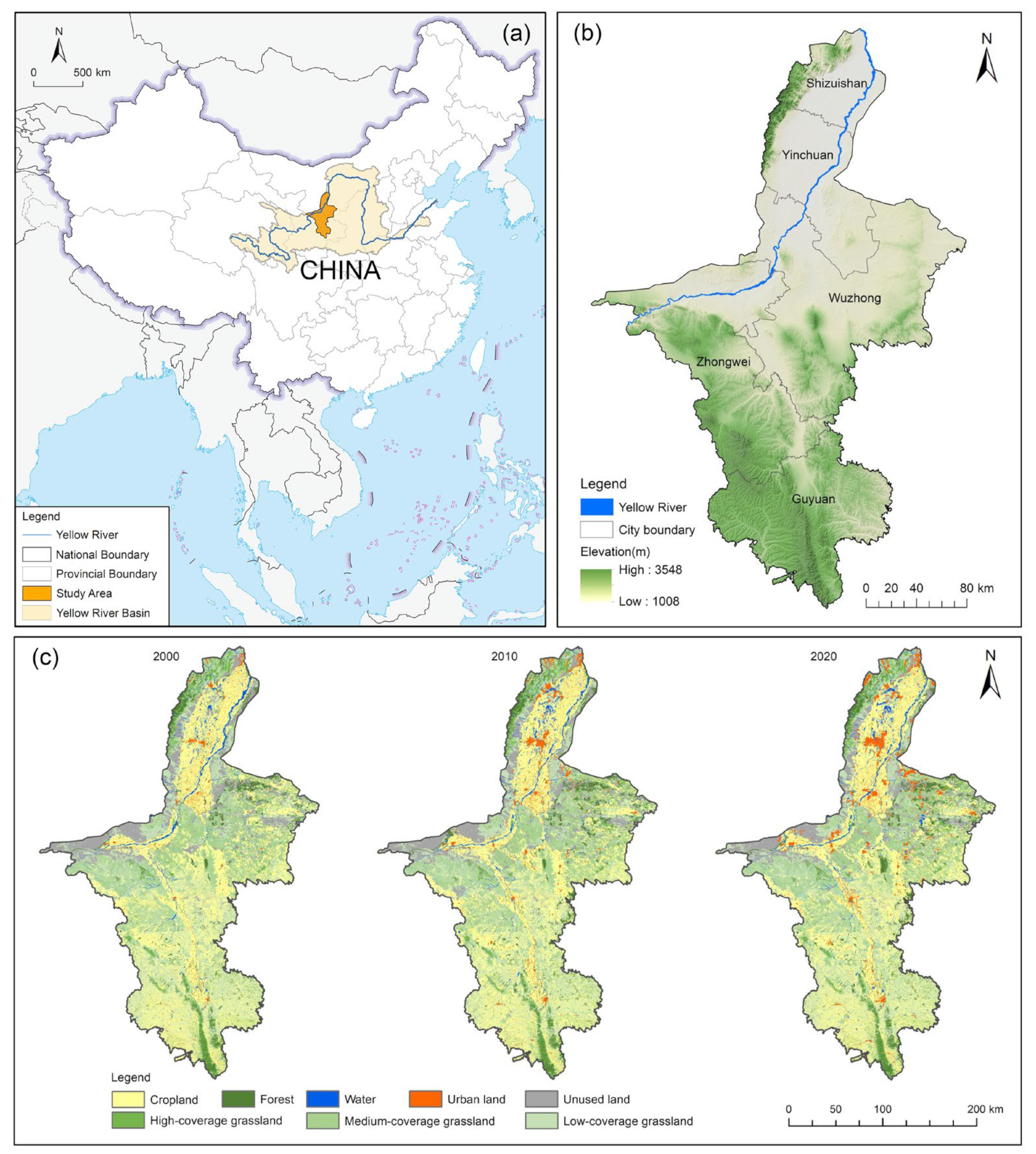
2.1. Study Area

NHAR is located in the center of China’s east–west axis, within the middle of the upper reaches of the Yellow River Basin (104°17′–107°93′ E and 35°14′–39°23′ N) (Figure 1). It spans approximately 460 km from north to south and 298 km from east to west, covering a total land area of 66,400 km². As of the end of 2019, the population was approximately 6.95 million, with an urbanization rate of 59.68%. NHAR is in the arid and semi-arid desert climate zone, with an annual precipitation of 289 mm, an annual evaporation of 1250 mm, and an average annual temperature ranging from 3.9 to 11.5 °C [38]. NHAR’s terrain descends from high in the south to low in the north, comprising the Yellow River alluvial plain in the north, the farming-pastoral transition zone in the middle, and the loess plateau in the south [39]. These geographical variances foster a diverse ecosystem and abundant natural resources. As the only province entirely within the Yellow River Basin, NHAR plays a significant role in the ecological preservation of the basin and the northwest region’s ecological security barrier, contributing greatly to the maintenance of the ecological stability and health of the Yellow River Basin. However, due to specific climatic characteristics and geographical divisions, NHAR’s environment is more sensitive and fragile. The rapid urbanization of its northern plain has resulted in landscape fragmentation, while the central arid area faces severe land desertification challenges [18]. Additionally, the issue of soil erosion in the loess-covered hills and gullies of the southern region is notably severe. This combination of factors elevates the risk of regional ecological degradation. Despite commendable progress in sand control, vegetation restoration, and soil and water conservation, leading to the recovery and improvement of the ecological environment, NHAR confronts ongoing ecological and environmental challenges. These include issues like water scarcity, desertification, and the inherent fragility and instability of its ecosystems.

2.2. Data Sources and Processing

This study collected data from the years 2000, 2010, and 2020, using a wide range of datasets related to land use data, digital elevation model (DEM), and the normalized difference vegetation index (NDVI), among others. Specific details regarding the data sources, precision units, and utilization of these datasets can be found in

Table 1. Data sources and description.

Data	Products	Related Uses	Time/Precision Unit	Data Sources
Land use data	China land use/cover remote sensing monitoring database	SC, WY, HQ, Resistance factor	2000, 2010, 2020 (30 m)	Resource and Environment Science and Data Center (http://www.resdc.cn, accessed on 25 November 2022)
Digital elevation model (DEM)	ASTER GDEM V3	SC, WY, Resistance factor	2009 (30 m)	Geospatial Data Cloud (http://www.gscloud.cn, accessed on 16 June 2022)
Normalized difference vegetation index (NDVI)	30 m annual maximum NDVI dataset in China from 2000 to 2020 [40]	SC, Resistance factor	2000, 2010, 2020 (30 m)	National Ecosystem Science Data Center (http://www.nesdc.org.cn, accessed on 8 September 2022)
Net primary productivity (NPP)	MOD17A3HGF	CS	2000, 2010, 2020 (500 m)	The Land Processes Distributed Active Archive Center (LPDAAC) (https://lpdaac.usgs.gov, accessed on 8 September 2022)
Soil data	China soil map based harmonized world soil database (HWSD) v1.2	SC, WY	1995 (1:1,000,000)	National Tibetan Plateau Data Center (http://data.tpdc.ac.cn, accessed on 25 September 2022)
Precipitation	1 km monthly precipitation dataset for China (1901–2020) [41]	SC, WY	2000, 2010, 2020 (1 km)	National Tibetan Plateau Data Center (http://data.tpdc.ac.cn, accessed on 25 September 2022)
Evapotranspiration	1 km monthly potential evapotranspiration dataset in China (1990–2021) [42]	WY	2000, 2010, 2020 (1 km)	National Tibetan Plateau Data Center(http://data.tpdc.ac.cn, accessed on 25 September 2022)
Population density	Population Counts/Constrained Individual Countries 2020 UN Adjusted	Resistance factor	2020 (100 m)	Worldpop Dataset (http://www.worldpop.org, accessed on 25 November 2022)
Nighttime light data (NTL)	VIIRS	Resistance factor	2020 (500 m)	Earth Observation Group (https://payneinstitute.mines.edu/eog/, accessed on 25 November 2022)
Transportation network	China fundamental geography database	Resistance factor	2019 (1:1,000,000)	National catalogue service for geographic information (www.webmap.cn, accessed on 11 June 2023)
Water network	China fundamental geography database	Resistance factor	2019 (1:1,000,000)	National catalogue service for geographic information (www.webmap.cn, accessed on 11 June 2023)
Administration boundary	China fundamental geography database	The boundary of the study area	2019 (1:1,000,000)	National catalogue service for geographic information (www.webmap.cn, accessed on 11 June 2023)

Note: HQ, SC, WY, and CS represent habitat quality, soil conservation, water yield, and carbon sequestration, respectively.

. According to our study purposes and regional landscape characteristics, land use types were classified into eight categories: cropland, forest, high-coverage grassland, medium-coverage grassland, low-coverage grassland, water, urban land, and unused land. To ensure consistency, all spatial data were transformed to a consistent spatial reference system (WGS_1984_UTM_Zone_48N), and raster data grids were harmonized to 30 m × 30 m.

3. Methods

The construction of ESP considering the stability of sources includes the following steps (Figure 2): (1) stable ecological sources are identified and classified based on the assessment of the ESI from 2000 to 2020, analysis of ESI change patterns, evaluation of sources stability, and landscape connectivity analysis; (2) a comprehensive resistance surface is constructed utilizing the SPCA method; and (3) the ecological corridors and strategic nodes are extracted using circuit theory, and an ESP that considers stability of sources is constructed. Based on this framework, recommendations for policy formulation and sustainable development are proposed.

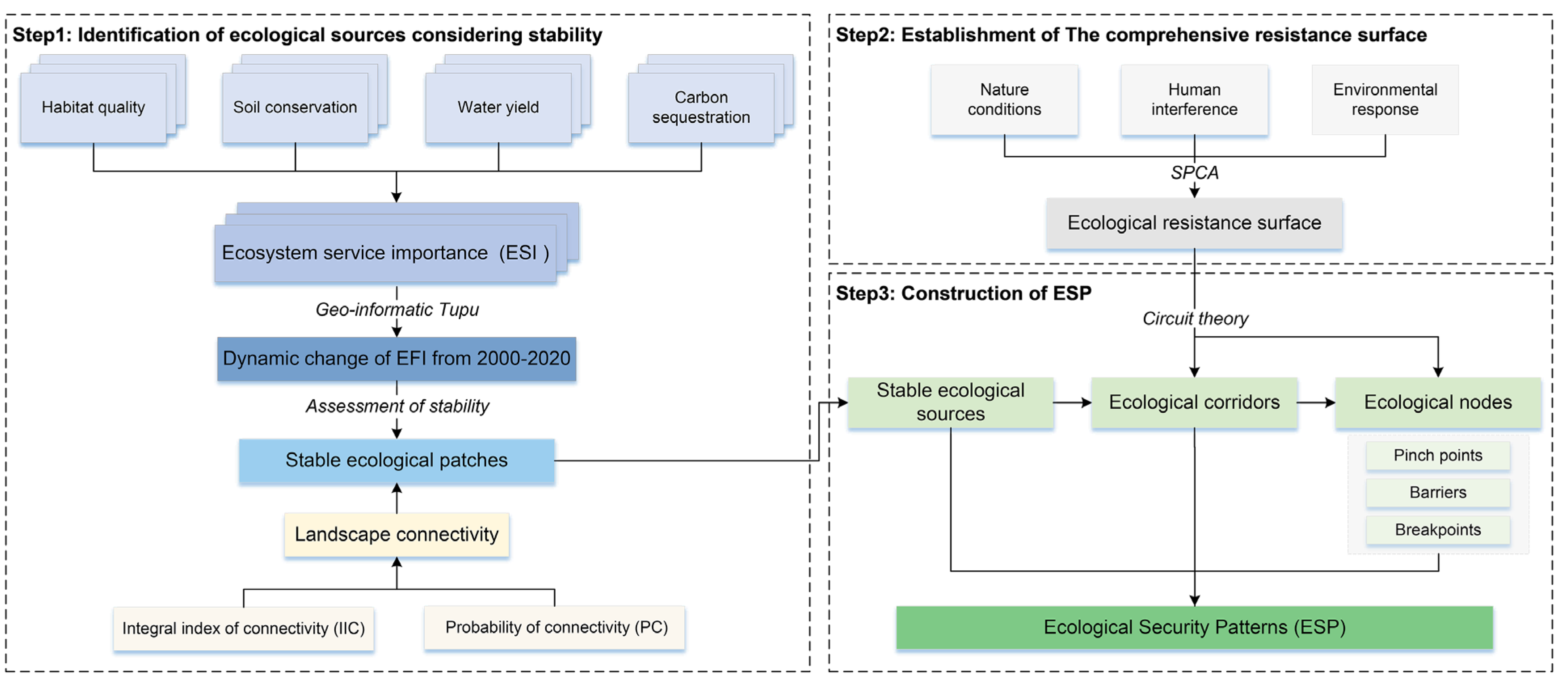
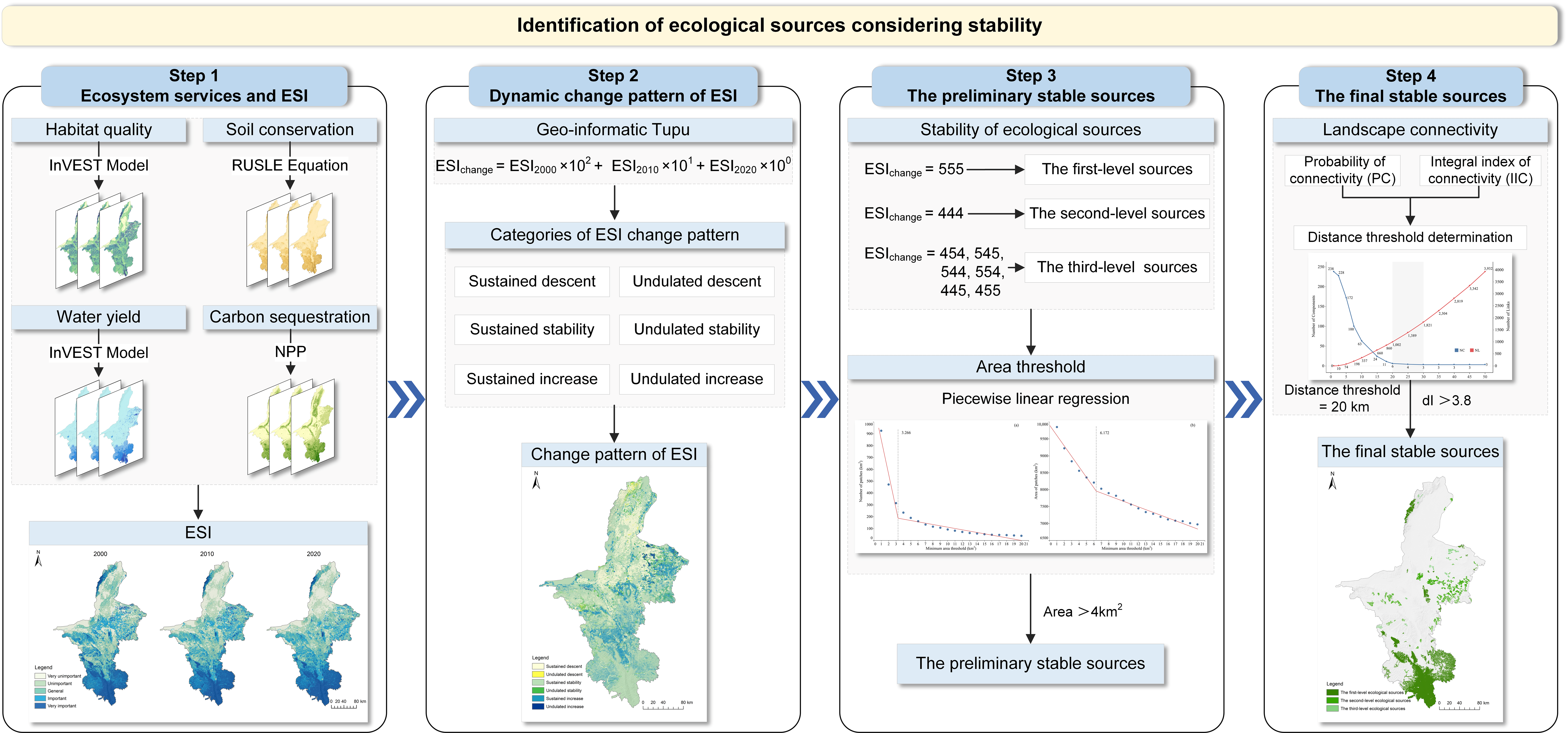
3.1. Identification of Ecological Sources Considering Stability

Ecological sources are important ecological patches that promote ecological processes, maintain ecosystem integrity, and provide essential ecosystem services, which are critical for ensuring regional ecological security [14,25]. However, due to the dynamic nature of external disturbances, these ecological sources may change over time. If a particular landscape remains consistent throughout the study period, it is considered a stable system [43]. In this study, we used the stability of ecological sources to characterize the ability of sources to maintain relatively stable ecological functions or services for a certain period in the face of external disturbances. The stability here is not absolute but relative stability during the research period. Therefore, the ability of ecological patches to consistently and stably deliver high-quality ecological functions and sustainable ecosystem services within a given timeframe should be a key criterion for identifying ecological sources. Additionally, these ecological patches should also maintain landscape connectivity, as higher landscape connectivity is more conducive to maintaining the stability of ecosystems [44]. To determine ecological sources, this study employed a comprehensive identification methodology that considers the stability of ecosystem function and landscape connectivity (Figure 3).

3.1.1. ESI Assessment for the Years 2000, 2010, and 2020

The ESI refers to the importance of services provided directly or indirectly by ecosystems, which serves as an indicator of ecological function to a certain extent. Evaluating the ESI can be used to identify key ecological patches that provide high-quality or high-quantity ecosystem services [3,14]. In consideration of the study area’s environmental characteristics and ecological functions, four ecosystem services were selected to assess the ESI: habitat quality, soil conservation, water yield, and carbon sequestration.

Habitat quality refers to the ability of the regional ecosystem to provide the necessary conditions for species survival, which is crucial for biodiversity protection [45,46]. High-quality habitats can provide optimal conditions for species survival, resulting in increased biodiversity. Habitat quality was estimated through the habitat quality module of the integrated valuation of ecosystem services and trade-offs (InVEST) model [47] as follows:

$$Q_{xj}=H_j(1-(\frac{D_{xj}^2}{D_{xj}^2+k^Z}))$$

(1)

where $Q_{xj}$ and $H_j$ represent the habitat quality and habitat suitability of grid x for land use type j, respectively; $D_{xj}$ indicates the habitat degradation degree of grid x; z is a constant value of 2.5; and k is the half-saturation constant. The resulting values range from 0 to 1, with higher values signifying superior habitat quality [23].

Soil conservation service refers to the ecosystem’s function in reducing soil erosion caused by water erosion through its structure and processes. The Revised Universal Soil Loss Equation (RUSLE) [48], which defines soil conservation as the difference between potential and actual soil erosion, was used to evaluate soil conservation. The formula is as follows:

$$A=R\times K\times LS\times (1-C\times P)$$

(2)

where $A$ is the average annual soil conservation (t/hm²·a); $R$ is the rainfall erosivity factor (MJ·mm/hm²·h·a); $K$ is the soil erodibility factor based on the mass percentage of sand, silt, clay, and organic carbon (t·hm²·h/(MJ·mm·hm²)); $LS$ is the slope length and steepness factor; $C$ is the cover and management factor; and $P$ is the erosion control practice factor.

Water yield refers to the yield of annual water contributing to human living, activities, and industrial water consumption [46]. The assessment of water yield often involves employing the water balance model, which quantifies the difference between regional precipitation and evapotranspiration as the ecosystem’s water yield. In this study, the water yield module of the InVEST model was used to evaluate the water yield as follows:

$$Y_{xj}=(1-\frac{{AET}_x}{P_x})\times P_x$$

(3)

where $Y_{xj}$ is the water yield value of grid x for land use type j (mm), ${AET}_x$ is the actual annual evapotranspiration of grid x (mm), and $P_x$ is the annual precipitation of grid x (mm). The specific parameters of habitat quality and water yield are detailed in Tables S1–S3 in Supplementary Materials. For detailed information regarding the verification of habitat quality, soil conservation, and water yield, please refer to Supplementary Materials.

Carbon sequestration is the biological process by which organisms convert inorganic carbon into organic compounds through photosynthesis [3]. Vegetation provides significant amounts of aboveground leaves for carbon sequestration and mediates the increase in greenhouse gases. Net primary productivity (NPP) can directly characterize vegetative productivity and serves as a commonly used proxy for assessing carbon sequestration in ecosystems [29].

The ESI was evaluated using a spatial overlay analysis based on the equal weight of the four ecosystem services’ estimation, and the specific formula is as follows:

$$ESI=HQ+SC+WY+CS$$

(4)

where HQ, SC, WY, and CS represent the standardized values for the four ecosystem services. The ESI value was divided into five grades (1—very unimportant, 2—unimportant, 3—general, 4—important, and 5—very important) using the quantile classification method, with the higher grade indicating the stronger ecological function of the patches and the greater importance of the patches to the ecosystem.

3.1.2. Construction of Change Monitoring Model for ESI

Change monitoring provides an objective means to measure the ESI within the research area at a specific time, which can be used to define the specific scopes of ESI change regions. Based on the geo-information Tupu theory [49], this study quantified the overall conversion process of the ESI from 2000 to 2020 and analyzed the temporal evolution and spatial distribution of the ESI. By categorizing the types of change patterns, this approach assessed whether the ESI remained stable, increased, or decreased between 2000 and 2020. The calculation formula is as follows:

$${ESI}_{change}={ESI}_{2000}\times {10}^2+{ESI}_{2010}\times {10}^1+{ESI}_{2020}\times {10}^0$$

(5)

where ${ESI}_{change}$ represents the codes of the ESI change patterns, while ${ESI}_{2000}$, ${ESI}_{2010}$, and ${ESI}_{2020}$ denote the ESI values for 2000, 2010, and 2020, respectively. Considering the complexity of change in the ESI, the change patterns were divided into six types based on the distinctive characteristics of ESI evolution. As shown in

Table 2. The categories of ESI change patterns from 2000 to 2020.

Types	Code Changes	Description
Sustained descent	211, 221, 311, 321, 322, 331, 332, 411, 421, 422, 431, 432, 433, 441, 442, 443, 511, 521, 522, 531, 532, 533, 541, 542, 543, 544, 551, 552, 553, 554	The ESI consistently decreased from 2000 to 2020.
Undulated descent	231, 241, 251, 312, 341, 342, 351, 352, 412, 413, 423, 451, 452, 453, 512, 513, 514, 523, 524, 534	The ESI exhibited a continuous decrease from 2000 to 2020, but there was an increasing or decreasing trend in 2010.
Sustained stability	111, 222, 333, 444, 555	The ESI remained stable from 2000 to 2020.
Undulated stability	121, 131, 141, 151, 212, 232, 242, 252, 313, 323, 343, 353, 414, 424, 434, 454, 515, 525, 535, 545	The ESI remained stable from 2000 to 2020, but there was an increasing or decreasing trend in 2010.
Sustained increase	112, 113, 114, 115, 122, 123, 124, 125, 133, 134, 135, 144, 145, 155, 223, 224, 225, 233, 234, 235, 244, 245, 255, 334, 335, 344, 345, 355, 445, 455	The ESI consistently increased from 2000 to 2020.
Undulated increase	132, 142, 143, 152, 153, 154, 213, 214, 215, 243, 253, 254, 314, 315, 324, 325, 354, 415, 425, 435	The ESI exhibited a continuous increase from 2000 to 2020, but there was an increasing or decreasing trend in 2010.

, an ${ESI}_{change}$ value of 345 indicates that the ESI shifted from the general state in 2000 to important in 2010 and ultimately to very important in 2020. These categories provide a structured framework for understanding the changes in the ESI over the specified periods.

3.1.3. Assessing the Stability and Identifying the Preliminary Stable Sources

Consistent with the common practice in the identification of ecological sources based on static snapshots, where patches classified as ‘very important’ or ‘important’ in ESI were typically considered ecological sources, this paper identified ecological patches with ESI change types 555 and 444 as potential stable ecological sources. These sources have consistently remained at the ‘very important’ and ‘important’ levels from 2000 to 2020, thus being considered stable in temporal changes, and this stability indicated their reliability in providing essential ecosystem services for regional development. Additionally, ecological patches that have undergone ESI changes but consistently remained within the top two importance categories were also considered candidate regions for stable ecological sources. These included types 454 and 545 (undulated stability), 544 and 554 (sustained descent), and 445 and 455 (sustained increase), where the functionality of these ecological patches may be slightly affected by external disturbances. The ecological sources were graded based on the ecological function importance and stability, with 555 being level 1, 444 being level 2, and 454, 545, 544, 554, 445, and 455 being level 3. Furthermore, ecological sources with sufficient scales can ensure the stability of ecological function [50]. The optimal area threshold for identifying ecological sources was determined using piecewise linear regression and overlay adjustment with protected areas, and ecological patches with an area exceeding 4 km² were regarded as the preliminary ecological sources. The determination of the optimal area threshold is shown in Figure S2 in Supplementary Materials.

3.1.4. Determination of Final Ecological Sources

Landscape connectivity refers to the degree to which a landscape facilitates or obstructs species movement and ecological flows [51]. It is an essential indicator for measuring ecological processes, and good connectivity can effectively enhance biodiversity preservation and the stability of ecological services [44]. The integral index of connectivity (IIC) and the probability of connectivity (PC) are common metrics for evaluating landscape connectivity. The IIC index assesses the importance of any landscape element or combination of landscape elements in maintaining overall connectivity. The PC index is defined as the probability of two species, located at random in the landscape, migrating into interconnected habitat areas, with this possibility of connectivity being related to the distance between habitat patches [52,53]. The formulas for IIC and PC are as follows:

$$IIC=\frac{\sum _{i=1}^n\sum _{j=1}^n\frac{a_i{a}_j}{1+n{l}_{ij}}}{A_L^2}$$

(6)

$$PC=\frac{\sum _{i-1}^n\sum _{j=1}^n{a}_i\times a_j{\times P}_{ij}^{\mathrm{*}}}{A_L^2},(0<PC<1)$$

(7)

where n is the total number of ecological patches, $n{l}_{ij}$ is the number of links in the shortest path between patches i and j, $a_i$ and $a_j$ are the areas of patched i and j, respectively, $A_L$ is the total landscape area, and $P_{ij}^{*}$ is the maximum product of dispersal probabilities along the links of all possible paths between patches i and j [54].

The delta values for the above index (dI) were used to represent the importance of existing patches in maintaining landscape connectivity and the change in overall connectivity that occurred after the destruction or removal of a patch [31]. The formula is as follows:

$$dI=\frac{I-I_{remove}}{I}\times 100\mathrm{\%}$$

(8)

where I is the index value (IIC and PC) when all of the patches are present in the landscape and $I_{remove}$ is the index value after the removal of a single patch, such as after the loss of a certain habitat patch [55]. A higher dI value indicates the higher connectivity importance of the patch.

The distance threshold is the maximum distance that ecological flows can reach within a certain range, and its determination is an important step for connectivity calculation [56,57]. This study determined the optimal range for the distance threshold by calculating the number of landscape links (NLs) and compositions (NCs) using various predefined thresholds. To further refine the distance threshold, the dIIC and dPC of the 20 largest preliminary ecological sources were evaluated at 1000 m intervals for trend analysis, and the final distance threshold was determined by comparing R² values and the highest correlation between dIIC and dPC. For detailed information, please refer to Figures S3 and S4 in Supplementary Materials. The dIIC and dPC values of all preliminary ecological sources were calculated with the final distance threshold of 20 km and a connection probability of 0.5, and the final ecological source was identified based on the patch importance assessed by the two indicators with equal weight. The landscape connectivity analysis was conducted using the ArcGIS 10.5 software plug-in module Conefor Inputs for ArcGIS 10. x and Conefer 2.6 software (http://www.conefor.org/, accessed on 12 December 2022).

3.2. Construction of the Comprehensive Resistance Surface

The ecological resistance surface reflects the resistance of species migration in space as well as the flow of material and energy within an ecosystem [3,15]. Recognizing that land use patterns and human activities significantly impact this resistance, a comprehensive resistance index system has been established incorporating three resistance factors: natural conditions, human interferences, and environmental response (

Table 3. The ecological resistance factors and resistance coefficient.

Resistance Classification	Resistance Factors	Resistance Coefficient
		1	2	3	4	5
Natural conditions	Elevation (km)	<1.3	1.3–1.5	1.5–1.8	1.8–2.1	>2.1
	Slope (°)	<6	6–12	12–20	20–30	>30
	Land use types	Forest/Water	High-coverage grassland/ Medium-coverage grassland	Cropland/ Low-coverage grassland	Unused land	Urban land
	Distance from rivers (km)	<1	1–3	3–5	5–10	>10
Human interference	Distance from railways (km)	>7.5	5–7.5	3–5	1–3	<1
	Distance from expressways (km)	>7.5	5–7.5	3–5	1–3	<1
	Distance from main roads (km)	>5	2–5	1–2	0.5–1	<0.5
	Nighttime light index	<3	3–12	12–27	27–50	>50
	Population density (People/km2)	<270	270–1200	1200–3000	3000–6200	>6200
Environmental response	FVC	>0.55	0.38–0.55	0.25–0.38	0.14–0.25	<0.14

). The natural conditions parameters included aspects such as elevation, slope, land use type, and distance from rivers, and the human interference factors were represented by distance from railways, expressways, and main roads (national and provincial), as well as the nighttime light index and population density. The fractional vegetation coverage (FVC) calculated by the NDVI was selected as the environmental response factor to reflect the vegetation resource utilization response to human activities. Incorporating these factors into the resistance index system enables a more comprehensive consideration of the ecological processes involving the flows of material, information, and ecology, both among different land use types and among patches of the same land use type [14]. The resistance factors were classified into five levels using the natural breakpoint method, in conjunction with relevant references. The corresponding resistance values were designated as 1, 2, 3, 4, and 5, with higher values indicating a greater level of resistance and 1 representing the lowest resistance.

To construct the resistance surface, SPCA was employed to determine the weight of each resistance factor within the comprehensive resistance index system. SPCA converts information from multiple raster layers into several principal component factors that retain the key information of the original factors by rotating the spatial coordinate axis of the characteristic spectrum [9,58]. This process avoids correlation and information redundancy among the factors, leading to a more rational allocation of weights for comprehensive evaluation indices, thereby enhancing the objectivity and comprehensiveness of weight assignment [25]. The SPCA in this study was conducted using the Principal Components tool in ArcGIS 10.5, and the formula is as follows:

$$R=\sum _{i=1}^m\sum _{j=1}^n{a}_{ij}{F}_j$$

(9)

where $a_{ij}$ is the jth principal component corresponding to the ith grid and $F_j$ is the eigenvalue contribution rate of the jth principal component. Generally, we selected only those principal components with cumulative variance contribution rates exceeding 90% [59].

3.3. Determination of Ecological Corridors and Ecological Strategic Nodes

3.3.1. Extraction of Ecological Corridors

Ecological corridors are important channels for species migration and ecological flows, typically appearing as linear or ribbon-shaped elements within the landscape [30,60]. These corridors could maintain the connectivity among ecological sources, thereby enhancing the stability of ecological functions [50]. The circuit theory has been widely applied to identify ecological corridors; it simulates species or energy movement in the landscape based on the characteristics of random walks of electrons in circuits [7,28], integrating all potential pathways between habitat patches and predicting the likelihood of successful species dispersal. In circuit theory, an ecological source is regarded as a node, the landscape as a conductive surface, and the species or energy as electrons. The heterogeneous landscape can be abstracted as a circuit composed of nodes and resistors, with 1 A current input from any source while other sources are grounded. The accumulated current value from one source to another is calculated by iterating through all the connections between ecological sources, reflecting the net number of times with which species or energy reaches the destination node through the corridors. The identification of ecological corridors was accomplished using the Linkage Mapper tool within ArcGIS 10.5. Additionally, the Centrality Mapper tool was employed to calculate current flow centrality to assess the importance of ecological corridors in maintaining overall network connectivity. The corridors were then categorized into three levels based on accumulated currents using the quantile method: key ecological corridors, important ecological corridors, and general ecological corridors.

3.3.2. Extraction of Pinch Points, Barriers, and Breakpoints

There are some key nodes in ecological corridors that play an effective control or promotion role in the ecological process, such as pinch points and barriers. Pinch points are high-flow key areas in the ecological process, and their degradation or loss may disrupt connectivity between source areas, thus demanding priority attention in ecological protection efforts [3]. Barriers are regions where landscape features obstruct the movement of species and ecological processes between ecologically important patches. Restoring these barriers can significantly enhance landscape connectivity [15]. Within the framework of circuit theory, pinch points are identified as areas with the highest accumulated current values within the corridors, while barriers are recognized as areas with the highest accumulated current recovery values. The identification of these key nodes was carried out through the application of the Pinchpoint Mapper and Barrier Mapper tools. The weighted distance of the corridor was set to 1000 m since the core positions and connectivity of pinch points would not be affected by changes in corridor width [29]. The moving window approach was used to determine the barriers, with a minimum search radius of 200 m, a maximum search radius of 1000 m, and a step size of 200 m. The natural breakpoint method was then applied to classify the results into three levels, with the highest level being designated as ecological pinch points and barriers, respectively. Furthermore, considering the potential hindrance posed by road networks to biological migration and ecological flow within ecosystems [5], intersections of the railways and expressways with corridors were regarded as the ecological breakpoints through overlay analysis.

4. Results

4.1. Spatial Distribution of Ecological Sources

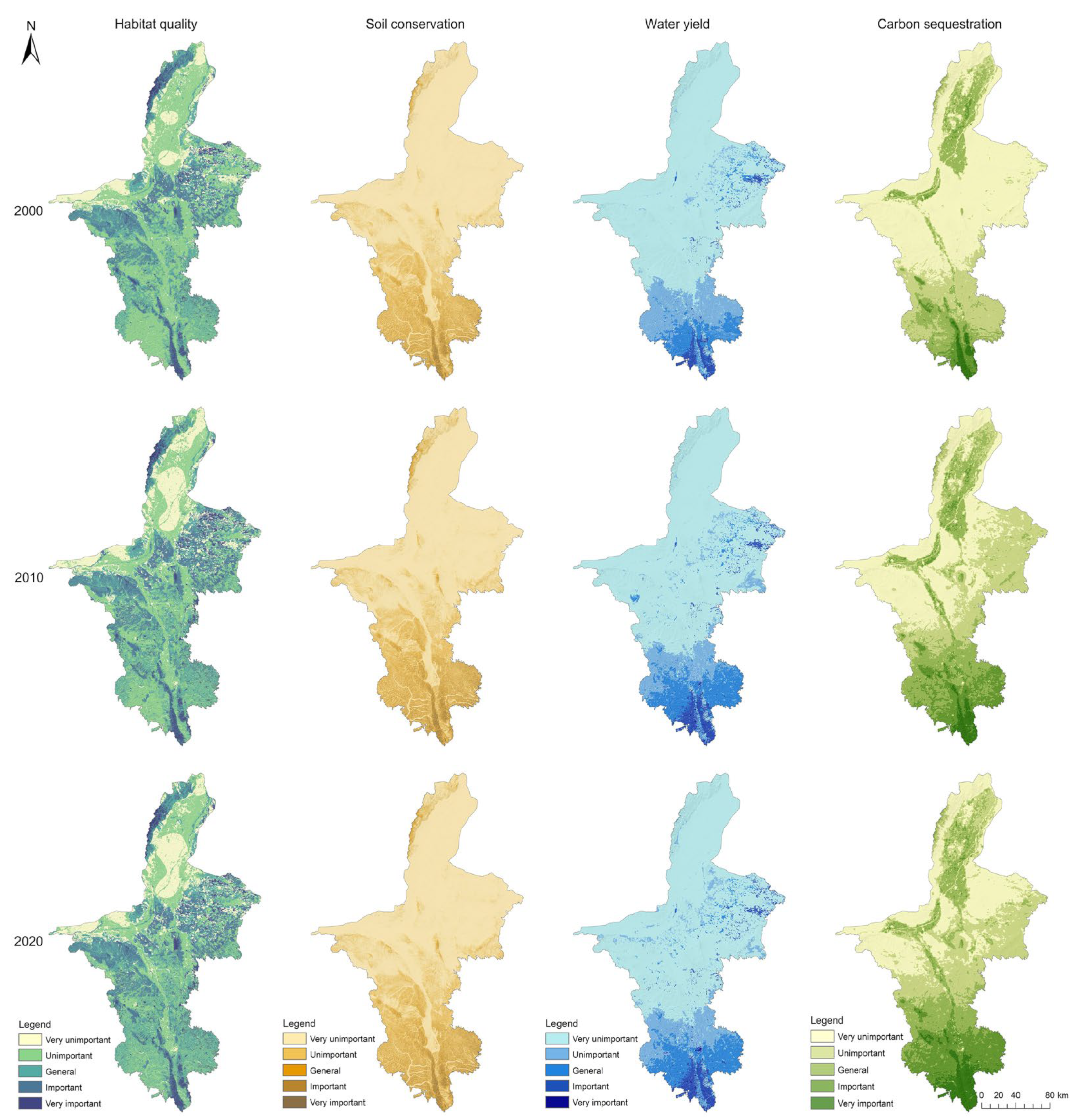
4.1.1. Spatial–Temporal Distribution of Ecosystem Services

According to the evaluation results of the four ecosystem services, it can be observed that these ecosystem services vary substantially in terms of both spatial and temporal scales (Figure 4). Areas with high habitat quality were primarily concentrated in the northern Helan Mountain region and the southern Liupan Mountain region, with scattered distributions in the central NHAR. As grassland was the dominant natural resource in the study area, certain regions with higher grass coverage also exhibited high habitat quality. The distribution of soil conservation was influenced by the combined effects of precipitation, topography, and vegetation. As a result, areas with high soil conservation were prominently located in the forests and grassland surrounding Helan Mountain and Liupan Mountain. High water yield areas were mainly distributed in the southern Liupan Mountain region and the eastern desert grassland area. However, due to climatic heterogeneity, water yield values were lower in the northern regions of NHAR. High-value carbon sequestration areas were primarily located in regions with substantial forest cover, such as Helan Mountain and Liupan Mountain, while cropland and dense grassland-covered areas also contributed significantly to carbon sequestration.

The study area experienced an overall increase in ecosystem services between 2000 and 2020. The habitat quality declined in the northern urban areas due to urban expansion, while other regions showed a steady improvement in habitat quality, with significant progress observed in Luo Mountain, which is located in the central region and the eastern desert areas. Although changes in the spatial variation of soil conservation were not readily evident over time, the total amount of soil conservation increased continuously, with a 29.87% increase in 2010 compared to 2000 and a 9.72% increase in 2020 compared to 2010. In terms of water yield and carbon sequestration, significant changes occurred over the past two decades. Water yield remained stable in the southern part of the study area, whereas notable increases were observed in the western and central regions. Concurrently, carbon sequestration displayed a clear gradient of improvement.

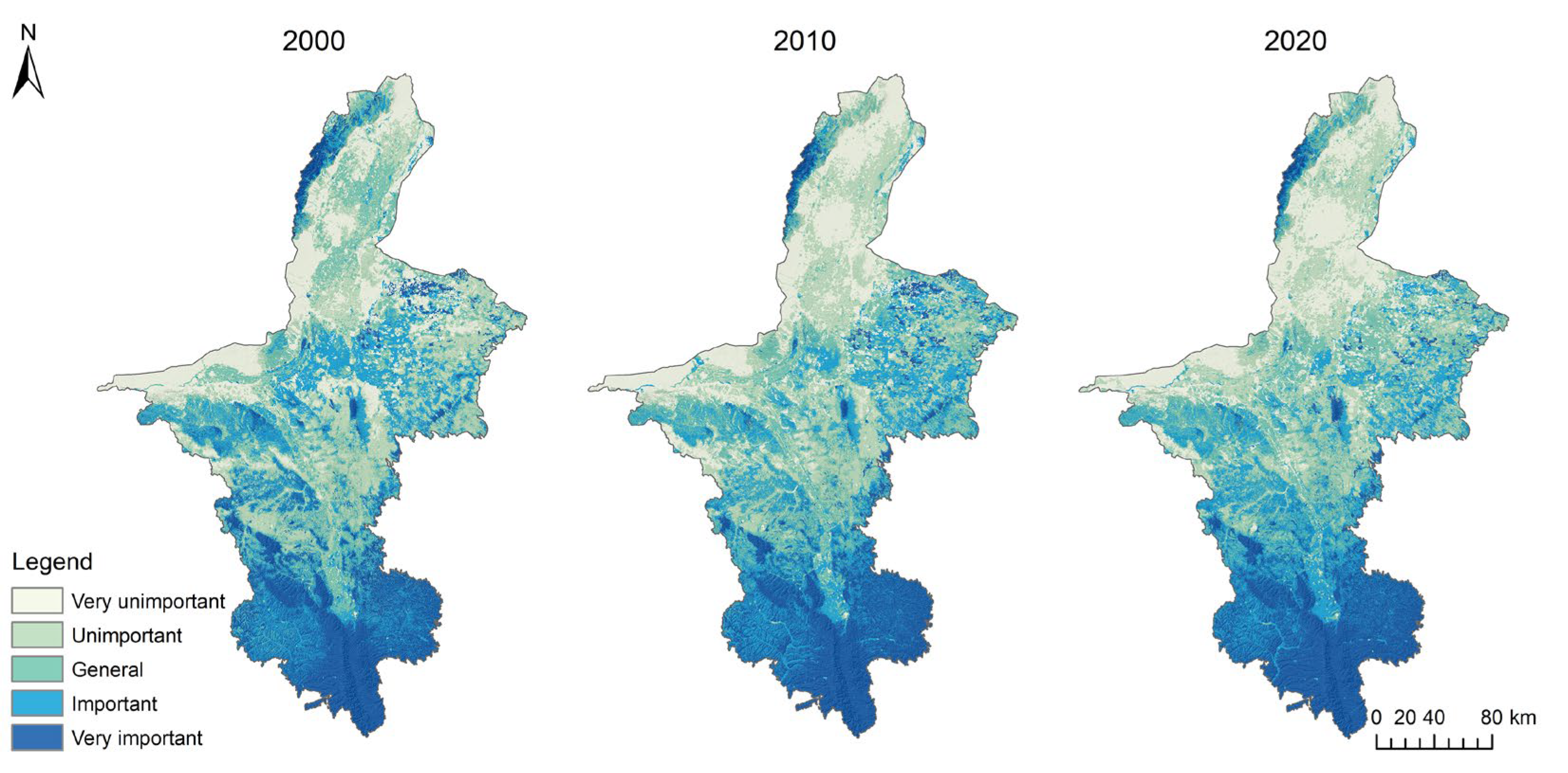
4.1.2. Spatial Patterns of the ESI

The spatial patterns of the ESI for the period of 2000 to 2020 are shown in Figure 5. Among the five levels of the ESI, the very unimportant level was mainly concentrated in the northern and northwestern regions of NHAR. The important level was primarily observed in the central and southern regions. The very important level was mainly distributed in the southern mountainous areas, the northern Helan Mountain region, and the central Luo Mountain region. These areas provided higher ecosystem services due to the presence of natural or semi-natural terrestrial ecosystems and protected areas. Additionally, the very important level displayed a dispersed distribution in the western and eastern regions of the study area, where these regions had high values of water yield and habitat quality. Although the overall spatial patterns of the ESI have remained relatively consistent over time, notable changes were observed in certain areas, such as the northern plain, the central Luo Mountain area, and the eastern desert area. This indicates the dynamic nature of the ESI and highlights the need for dynamic management and conservation of these regions to ensure the long-term sustainability of these fundamental services.

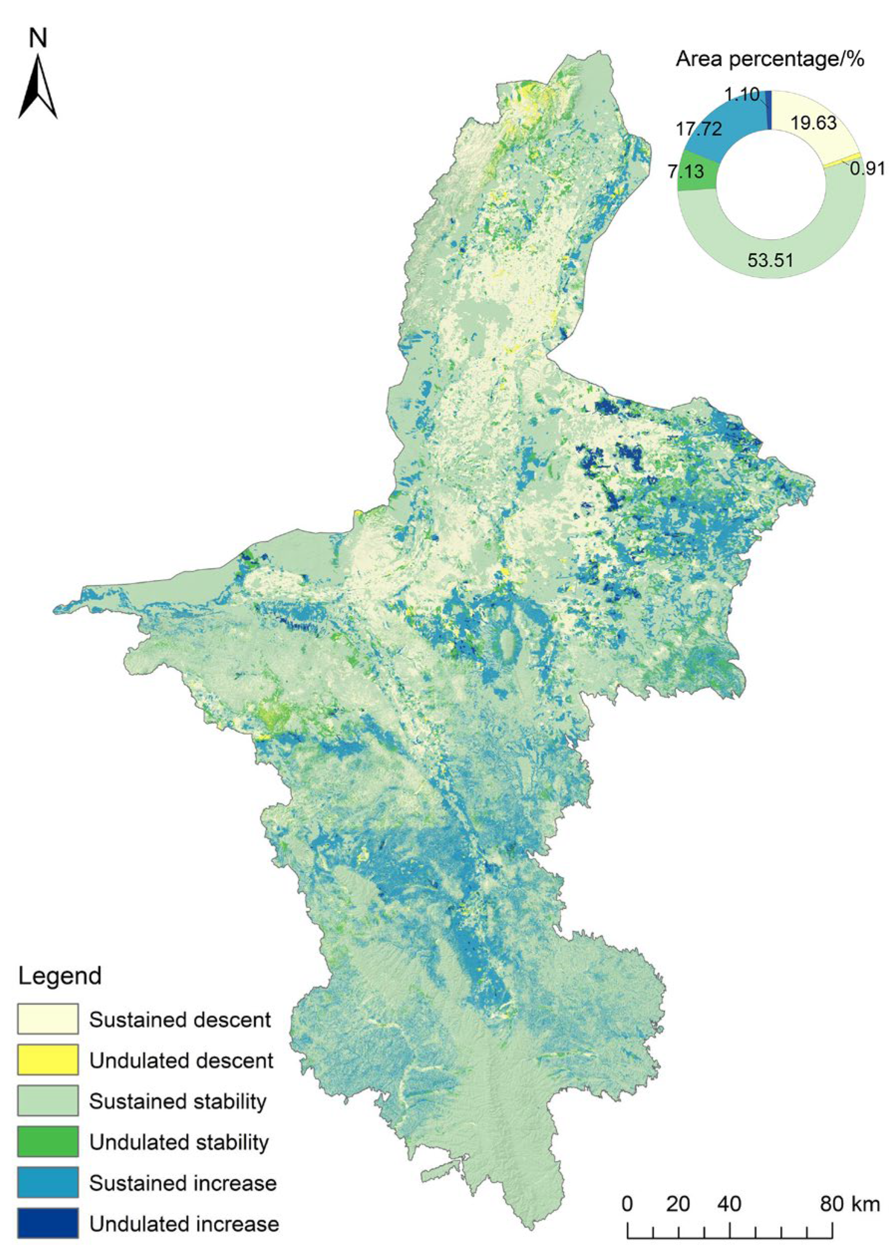
4.1.3. Overall Change Patterns of the ESI

The overall change patterns of the ESI from 2000 to 2020 are shown in Figure 6. A significant portion, accounting for 60.64% of the study area, maintained its original ESI level (sustained and undulated stability type), with the sustained stability region accounting for 53.31%. These areas were primarily concentrated in desert grasslands, urban areas, and regions with high vegetation coverage, such as Helan Mountain and Liupan Mountain. The ecosystems in these regions were at two extremes and displayed good stability against external interference. The areas with an increased ESI (sustained and undulated increase) covered 18.82% of the study area and were mainly observed in the northern coastal region of the Yellow River, the desert grassland in the western and eastern parts, the central region near the Luo Mountain, and the south-central part. The rise in the ESI within these areas may be attributed to the development of regional green industries, the implementation of ecological governance and conservation along the Yellow River, and the effective control of desertification in central parts. The areas with a decreased ESI (sustained and undulated descent), totaling 20.54% of the total area, were mainly concentrated in urban areas in the northern and central parts of NHAR. The past 20 years have witnessed the rapid growth of urbanization in China, and urban expansion inevitably has a direct or indirect impact on the regional ecological environment. The urban expansion pattern in northern and central NHAR is mainly edge expansion [2]. However, the ESI was increasing in certain places on the edge of urban areas, implying that incorporating regional ecological protection into urbanization construction may help to coordinate the conflict between protection and development.

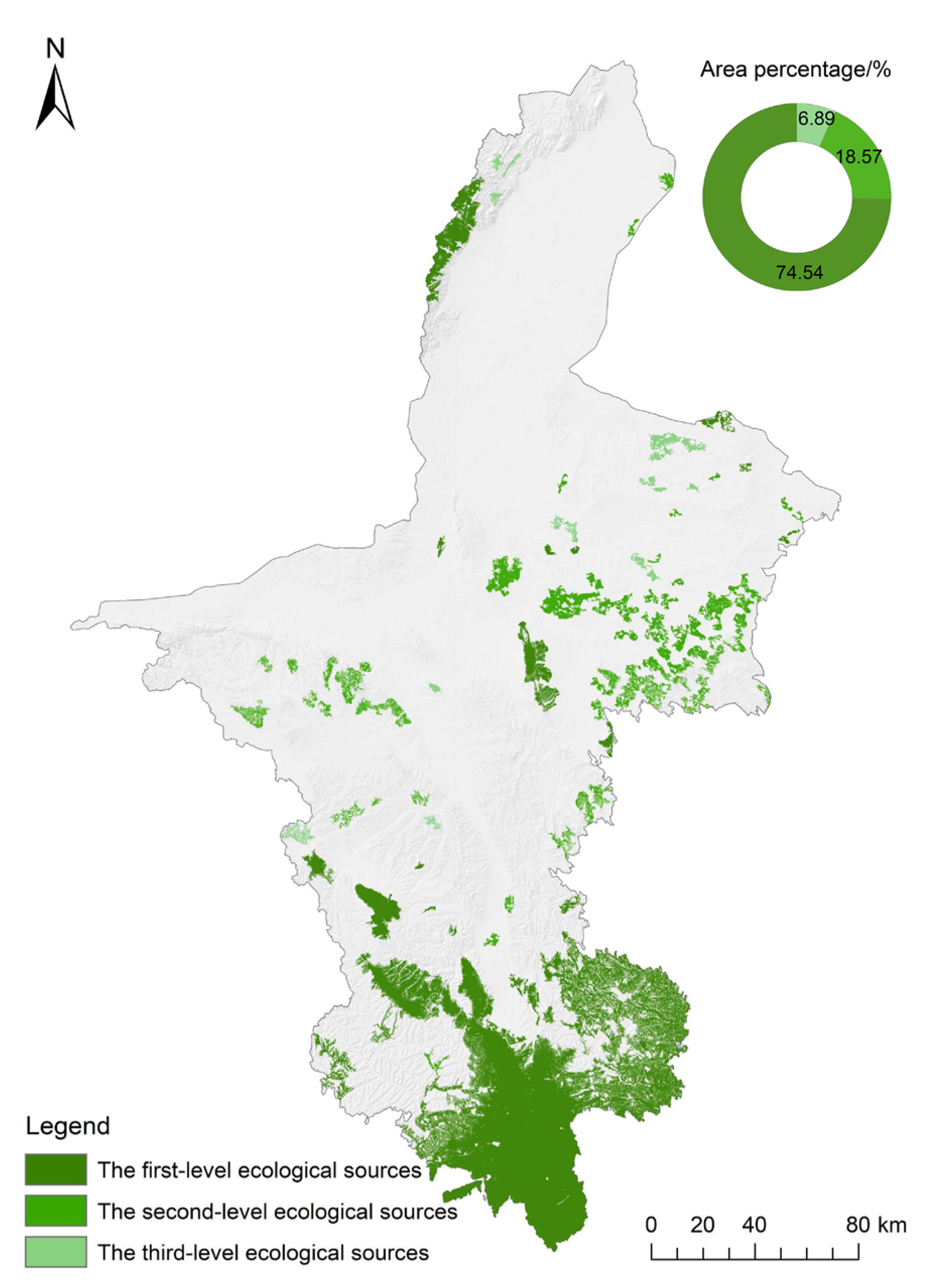
4.1.4. The Distribution Characteristics of Ecological Sources

By extracting stable ecological patches larger than 4 km² in size, a total of 238 preliminary ecological sources were identified, and patches with connectivity importance greater than 3.8 were screened to finally obtain 93 stable ecological sources (Figure 7). These ecological source areas accounted for 16% of the total study area, and their distribution was unbalanced. Most ecological sources were located in the southern, central, and eastern regions, while the ecological sources in the northern and western parts were relatively scarce and more dispersed. Within these stable ecological source areas, the first and second-level source areas accounted for 93% of the total source area, with the first level comprising 75.54%. The first-level sources were primarily located within natural reserves such as Helan Mountain, Luo Mountain, Liupan Mountain, Nanhua Mountain, Huoshizhai, Yunwu Mountain, Dangjiacha, the Qingtongxia Reservoir Wetland, and Haba Lake. The second-level sources were mainly distributed in the western and eastern regions of the study area, while the third-level source areas were scattered across the northern, northeastern, and central-southern regions of the study area. In general, the stable ecological sources in NHAR exhibited a spatial pattern with the first-level ecological sources of Helan Mountain, Luo Mountain, and Liupan Mountain as the core, the second-level ecological sources dominating the eastern and western wings, and the third-level ecological sources scattered between the first- and second-level sources.

The composition analysis of land use types in ecological sources showed that the primary land use types in stable ecological sources were grassland, forest, and cropland. Grassland covered 61.34% of the total source area, followed by forest, which covered 16.58% of the area. The grasslands were further classified into high, medium, and low coverage types, accounting for 6.43%, 31.73%, and 23.18% of the ecological source area, respectively, demonstrating that medium-coverage grassland emerged as the most prominent land use type that contributes to the ecological sources. NHAR exhibits typical characteristics of a desert-to-grassland ecosystem transition, with grassland being the most abundant and important terrestrial ecosystem [39]. Under conditions of climate and limited water resources, medium-coverage grassland provides a more suitable habitat for the biota of the desert/grassland. From 2000 and 2020, the overall structure of land use in ecological sources remained relatively stable, with noticeable changes occurring in specific sources (Figure 8). The most common types of changes observed involve mutual transformations between forest and grassland, such as the shifts from predominantly grassland to predominantly forest in sources No.22, No.24, No.25, and No.47, the changes from grassland to forest in sources No.61 and No.64, and the changes from medium-coverage grassland to high-coverage grassland in source No.86. Furthermore, although cropland provides space for species diffusion in natural ecosystems [24], land use changes in sources containing cropland, such as in sources No.1, No.3, and No.8, maybe more complicated due to their heightened susceptibility to human activities. Therefore, in the process of ecological protection and restoration, it is imperative to reinforce the ecological function of grassland, prioritize the assessment and management of cropland quality, and promote the combination of sustainable agriculture and species protection to enhance the safety and stability of natural ecosystems [61]. In general, there were more significant changes in the land use composition of ecological sources from 2000 to 2010 compared to 2010 to 2020, indicating relatively stable land use in ecological sources from 2010 to 2020.

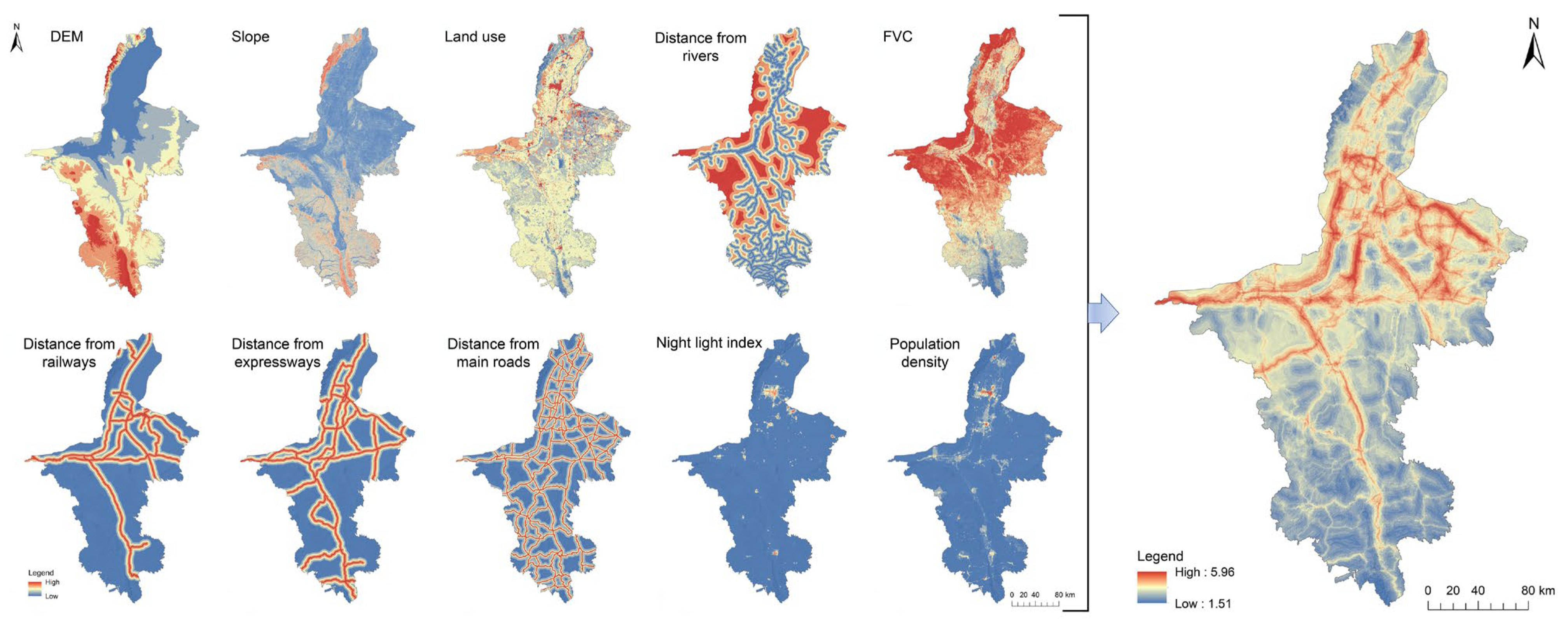
4.2. Analysis of Ecological Resistance Surface

The SPCA results showed that the cumulative contribution rate of the first seven principal components reached 93.423%, effectively summarizing the resistance composition within the study area.

Table 4. Factor loading matrix of spatial principal components.

Index Type	Restraint Factors	PC1	PC2	PC3	PC4	PC5	PC6	PC7	PC8	PC9	PC10
Natural conditions	Elevation	−0.452	−0.204	0.449	0.025	0.099	0.015	0.113	0.726	0.043	0.005
	Slope	−0.321	−0.226	0.268	−0.216	0.343	0.558	0.195	−0.510	0.002	−0.008
	Land use	0.122	0.031	−0.106	0.103	−0.156	−0.039	0.957	0.028	−0.138	−0.013
	Distance from rivers	−0.081	0.720	0.588	0.118	0.047	−0.243	0.046	−0.226	0.019	0.000
Human interference	Distance from railways	0.498	−0.030	0.056	−0.202	0.796	−0.201	0.077	0.160	−0.035	−0.003
	Distance from expressways	0.535	−0.128	0.479	−0.461	−0.451	0.209	−0.032	0.080	−0.024	0.002
	Distance from main roads	0.337	−0.280	0.287	0.818	0.037	0.202	−0.081	−0.069	−0.047	0.014
	Night light index	0.042	−0.013	−0.012	0.006	−0.003	−0.006	0.080	−0.019	0.526	0.845
	Population density	0.070	−0.034	−0.005	0.031	−0.012	−0.019	0.100	−0.023	0.835	−0.534
Environmental response	FVC	0.131	0.539	−0.232	0.062	0.083	0.709	−0.030	0.351	0.034	−0.007
Principal component eigenvalues	-	1.411	0.903	0.504	0.459	0.378	0.300	0.265	0.211	0.065	0.021
Cumulative contribution rate (%)	-	31.221	51.208	62.370	72.532	80.904	87.552	93.423	98.102	99.534	100

presents the original evaluation factor loads corresponding to each principal component. Among these components, distance from railways and expressways had advantages in the first principal component, demonstrating that human interference was the most important factor contributing to resistance surface. The load values of distance from rivers and FVC greatly exceeded the contributions of other factors in the second principal component, which reflected the contribution of natural conditions and environmental response to ecological resistance. In the third primary component, the distance from rivers, distance from expressways, and elevation had relatively higher load values, with the contribution of elevation being comparable to that of the distance from expressways. Distance from main roads and distance from railways contributed the most to the fourth and fifth principal components, respectively. FVC and slope exhibited the highest contributions for the sixth principal component, while land use was the dominant factor in the seventh principal component. Moreover, the load effects of the nighttime lighting index and population density were not representative of the ecological resistance surface among the seven principal components. Overall, the formation of ecological resistance in the study area was the result of a comprehensive effect of natural conditions, human interference, and environmental response factors, with FVC having a relatively weaker influence compared to human interference and natural conditions. Considering the study area’s arid and semi-arid characteristics, as well as the fragile ecological environment, water sources played a crucial role in facilitating species migration and ecological flow, and activities related to transportation that promote economic development may increase the resistance of ecological flow [31].

The ecological resistance surface was calculated according to the first seven principal components and their contribution rate (Figure 9). Generally, the average ecological resistance of NHAR was 3.24, with notable regional variations. The high resistance areas were mainly concentrated in the urban areas along the Yellow City Belt, the deserts in the west and east, and the urban areas in the central and southern parts along the expressways. The low resistance areas were primarily distributed in the northern part of NHAR, including the Helan Mountain region and the region along the Yellow River, as well as the central-southern and southern sections of the study area. The low-value areas were clearly separated from the high-value areas, resulting in a resistance distribution pattern characterized by low resistance in the south, high resistance in the middle, and intermediate resistance in the north.

4.3. Construction of the ESP

The ESP in NHAR consisted of ecological sources, ecological corridors, pinch points, barriers, and breakpoints (Figure 10). A total of 234 ecological corridors were identified, with an average length of 17.780 km (ranging from 0.042 to 150.634 km) and a total length of 4160.67 km. The ecological corridors effectively connected the northern, central, and southern parts of NHAR, establishing stable ecological linkages and providing the structural foundation for material circulation and energy flow within the ecosystem. Spatially, these corridors were densely distributed and cobweb-shaped in the central and southern regions, while the opposite was observed in the north. Key ecological corridors, totaling 691.45 km (16.6% of the total corridor length), were mainly located in the central and southeastern parts of the study area. The total length of important ecological corridors was 1888.66 km (45.4% of the total corridor length), with a majority located in the eastern and western regions of the study area. The general ecological corridors, with a combined length of 1580.56 km (38% of the total corridor length), were mainly distributed in the north, east, and south, connecting the ecological sources in these regions to form three densely interconnected network clusters. Overall, each level of ecological corridor played a distinct role in regional ecological connectivity. Key ecological corridors were the backbone of the overall ecological connections, ensuring the integrity and continuity of ecological processes in both north–south and east–west directions within the study area. Important ecological corridors primarily facilitated connections between different levels of ecological sources, providing essential pathways for species movement and ecological flows. Meanwhile, general ecological corridors, although relatively short, performed an important function in connecting clusters of ecological sources, thereby improving local connectivity and maintaining biodiversity.

Ecological strategic nodes identified in this study include pinch points, barriers, and breakpoints. A total of 231 pinch points were identified, covering an area of 1141.46 km². These pinch points were primarily concentrated in the central axis of the study area, and the land use types involved were cropland, medium-coverage grassland, and low-coverage grassland. Notably, these pinch points were primarily observed within key ecological corridors, particularly the north–south corridors linking the northern and central regions, as well as the east–west corridors within the south-central region. Due to the constraints of roads and residential areas, these regions lacked viable, low-cost alternatives and required focused protection. Furthermore, our study identified 45 ecological barriers, covering a total area of 175.4 km². They were mainly located in low-coverage grassland and bare land within the eastern and western regions of the study area, causing certain resistance to ecological flows. Future actions are recommended to improve and restore these barriers to optimize the connectivity between ecological resources. Additionally, 154 breakpoints were identified, with over 56% being influenced by expressways. These points were concentrated in densely populated areas with extensive transportation networks, such as cities or towns, indicating a high probability of ecological corridor fragmentation, and should be prioritized for future ecological restoration.

5. Discussion

5.1. Application of ESP Framework Considering Source Stability

Identifying the ecological sources is the most critical step in constructing ESPs, and the ecological sources’ location significantly influences the ESPs’ spatial structure. Ecological importance assessment based on ecosystem services is the most commonly used method for identification of ecological sources [62]. With the rapid environmental changes, it is evident that ecosystem services are dynamic. The results revealed that all four ecosystem services exhibited temporal and spatial heterogeneity, with habitat quality, water yield, and carbon sequestration showing noticeable dynamic changes. Despite habitat quality in the northern region inevitably declining due to urban expansion, the water yield and carbon sequestration clearly increased. Previous studies have underscored the significant influence of policy-driven human activities on ecological processes, both in promoting and inhibiting them [16]. A series of ecological restoration plans implemented in this area, such as converting cropland to forests and grasslands, may have played a significant role in enhancing regional ecosystem services [63].

However, the dynamic growth of ecosystem services, influenced by various land use types, landscape patterns, and development intensity, increases the difficulty of source identification [58]. Our results illustrated significant changes in the spatial distribution of the ESI over time. As regional ecological security is a dynamic process, the ESP constructed by identifying the sources with multi-period ESI static snapshots helps understand the spatial variation of regional ecological risks and the evolution process of an ESP [23,64]. However, this method may ignore the dynamic nature of sources over time, which may lead to potential deviations in ecological management policy formulation. The stable sources identified in this study can ensure a sustained supply of high-level ecosystem functions and resistance to external interference. They also have reliable ecological integrity and connectivity to support a more stable flow of energy, materials, and services among ecological patches. Ecological protection and restoration are inherently long-term, sustainable processes. Consideration of source stability can assist decision-makers in effectively determining core or key areas that can remain stable in dynamic changes, as well as providing additional information to identify priority areas in ecological protection and restoration.

The spatial superposition of stable ecological sources and nature reserves showed that first-level ecological sources were primarily distributed across major nature reserves, indicating that nature reserves remain an essential area for providing stable and high-quality ecosystem services for a long time. The European Union (EU) Biodiversity 2030 Strategy aims to protect at least 30% of terrestrial areas by 2030 [65], implying the need for expansion of a protective scope [66]. However, focusing solely on the extent of protected areas without evaluating their effectiveness may hinder the achievement of conservation goals [67]. It has been reported that approximately one-third of the world’s protected areas experience significant human pressures, highlighting the necessity of mitigating these pressures to enhance the effectiveness of these areas [31,68]. Stable ecological sources can offer direction for the reserve’s future development, serving as the core areas or priority areas for reserve planning with strict control measures, which will help improve protection effectiveness within the constraints of limited resources, thus realizing the future protection vision.

The prioritization issue is a rather common topic of conservation science when limited economic resources necessitate the identification of sites that offer maximum benefits through protection [69]. The construction of ESPs is beneficial in determining priority areas for protection within resource planning and management, as well as maintaining the minimum ecological security of the region. However, due to abrupt climate change and rapid urbanization, ecological sources and corridors may be occupied by non-ecological land, which is not conducive to the long-term stability of the ESP [70]. Those ecological sources capable of consistently providing stable ecosystem services contribute to ensuring the sustained operation of the ESP, and thus, they can be considered the ‘backbone’ of a sustainable landscape. An ESP constructed based on stable sources has reliable integrity and connectivity, which can be regarded as the ‘bottom line’ within the ecological bottom line. On the one hand, it is a fundamental protection requirement or potential goal for regional ecological protection, serving as the basis for expanding and optimizing key protected areas. On the other hand, any human activities that disrupt this potential goal may lead to discordance between ecological protection and economic development. Therefore, the steady state of ESPs characterized by source stability is useful for early warnings of regional ecological security. Furthermore, ecological conservation increasingly focuses on core functions and services to enhance cost-effectiveness [34]. The ESP framework established in this study can contribute to rationally allocating and conserving ecological protection costs, which is critical for future ecological protection and restoration planning.

5.2. Management Implications Based on the Identified ESP

Achieving high-quality development and protecting land space required the preservation and responsible utilization of ecological space. A sustainable ESP can provide a fundamental guide for ecological space management and contribute to enhancing regional ecological conservation and sustainable development. This study found that stable ecological sources are unevenly distributed, with fewer sources in disturbed areas, particularly in the northern and western regions. These areas are surrounded by three deserts, making them susceptible to the influence of natural factors, potentially impacting long-term ecosystem stability. Human activities and urbanization significantly impact the function and services of regional ecosystems, subsequently affecting the regional ecology’s balance [14]. Therefore, as policies and plans are proposed and implemented, it is crucial to consider the stability of ecological landscape elements and scientifically harmonize the interplay of ecology, production, and living space to achieve the multiple goals of improving ecological protection, driving economic and social development, and fostering human well-being, which is especially important in ecologically fragile areas.

It is noteworthy that the edges of ecological patches are more prone to fragmentation under disturbance, leading to habitat loss and reduced ecological functions. In contrast, the core areas of ecological landscapes, which are usually better protected, can provide stable and reliable ecological services. Therefore, the stability-based classification method for sources can effectively enhance the formulation of targeted ecological protection policies. Specifically, first-level sources, providing stable and high-quality ecological functions, should be considered core areas of nature reserves and receive the highest priority protection. The primary focus in these areas should be on maintaining the stability of existing ecological functions. Establishing ecological buffer zones around these sources can reduce human disturbances to the core areas, thus preserving the integrity and functionality of critical ecosystems from degradation. For second-level sources, which are constrained by the environmental background of the study region, measures suitable for local conditions should be adopted to improve ecological functions or services, such as selecting suitable drought-resistant vegetation for ecological restoration, to ensure the long-term stability of the ecosystem. Furthermore, the third-level sources, possessing the potential to develop into higher-level source areas, flexible management and restoration strategies, should be implemented for these areas, with a focus on monitoring and evaluating changes in ecological functions, recognizing the impacts of various disturbances, and emphasizing the enhancement of the ecosystem’s resilience.

Ecological corridors function as vital bridges connecting ecological sources, effectively facilitating ecological processes [2,52]. This study’s findings emphasized the role of ecological corridors in establishing close ecological relationships among stable ecological sources. Considering the geographical layout of NHAR, which is characterized by being short from east to west and long from north to south, the key corridors were critical for maintaining landscape connectivity. The north–south key corridors connected the ecological sources of Helan Mountain in the north to Luo Mountain in the middle, while the east–west key corridors bridged the sources separated by residential areas in the central and southern regions. These corridors subsequently connected with Liupan Mountain in the south, forming an ESP with Helan Mountain–Luo Mountain–Liupan Mountain as the core sources. Notably, the ecological sources within these ‘Three Mountain’ regions were also classified as first-level sources, underlining their significance in preserving the stability and integrity of the regional ecosystem. The 14th Five-Year Plan [71] designates NHAR’s ‘One River and Three Mountains’ region as a pivotal area for ecological system construction, protection, and restoration projects. The ‘Three Mountains’ are crucial ecological security barriers, with specialized ecological protection and restoration plans having been formulated for each of them. Although ‘Three Mountains’ serve diverse ecological functions due to their distinct environmental characteristics, they occupy a central ecological position as the core ecological sources of northern, central, and southern parts of NHAR. Thus, it is recommended to continually deepen ecological protection and restoration efforts for the ‘Three Mountains’ to promote their radiation effect while enhancing the protection of important and general corridors to strengthen the connections between the ‘Three Mountains’ and surrounding ecological sources.

Several ecological nodes that restrict and hinder ecosystem connectivity have been identified as the potential landscape basis for regional ecological protection actions. These pinch points were primarily observed within key ecological corridors, emphasizing the importance of protecting these key corridors. Available habitats, such as steppingstones, can be placed along long key corridors to reduce spatial distance and enhance the ecosystem’s flexibility. Furthermore, the impact of road construction on ecological network connectivity has been a focal point in recent research, as roads may obstruct species migration or alter migration routes [72]. The distance from railways, expressways, and main roads was found to contribute significantly to the high resistance values in this study. This implies the need for close attention to the impact of roads on ecological resistance, the restoration of ecological breakpoints formed by the intersection of ecological corridors and roads, and the strengthening of the development of green infrastructure along transportation arteries to improve the connectivity and stability of the ecosystem.

6. Conclusions

In ecologically fragile regions, the impacts of climate change and human activities on ecosystems are particularly pronounced, directly influencing the maintenance of regional ecological security. Constructing an ESP for these fragile areas aids in identifying and protecting key regions, thereby enhancing the integrity and stability of natural ecosystems. This study integrated the evaluation of ESI change patterns, the SPCA method, and circuit theory to propose an ESP identification framework that prioritizes source stability, providing a novel approach for the construction of regional ESPs in fragile ecological areas. The main results are as follows:

(1)

A total of 93 stable ecological sources were identified in the NHAR and primarily located in its southern, central, and eastern regions. The dominant land use types within these sources included grassland, forest, and cropland. These sources were critical for regional ecological conservation, providing the region with stable and high-quality ecosystem services.

(2)

The ecological resistance surface was collectively shaped by natural conditions, human disturbance, and environmental response factors, with the impact of natural conditions and human disturbances being particularly significant. The distribution of resistance surfaces showed significant spatial variation, with high resistance values mainly concentrated in urban areas, regions with dense road networks, and desert zones.

(3)

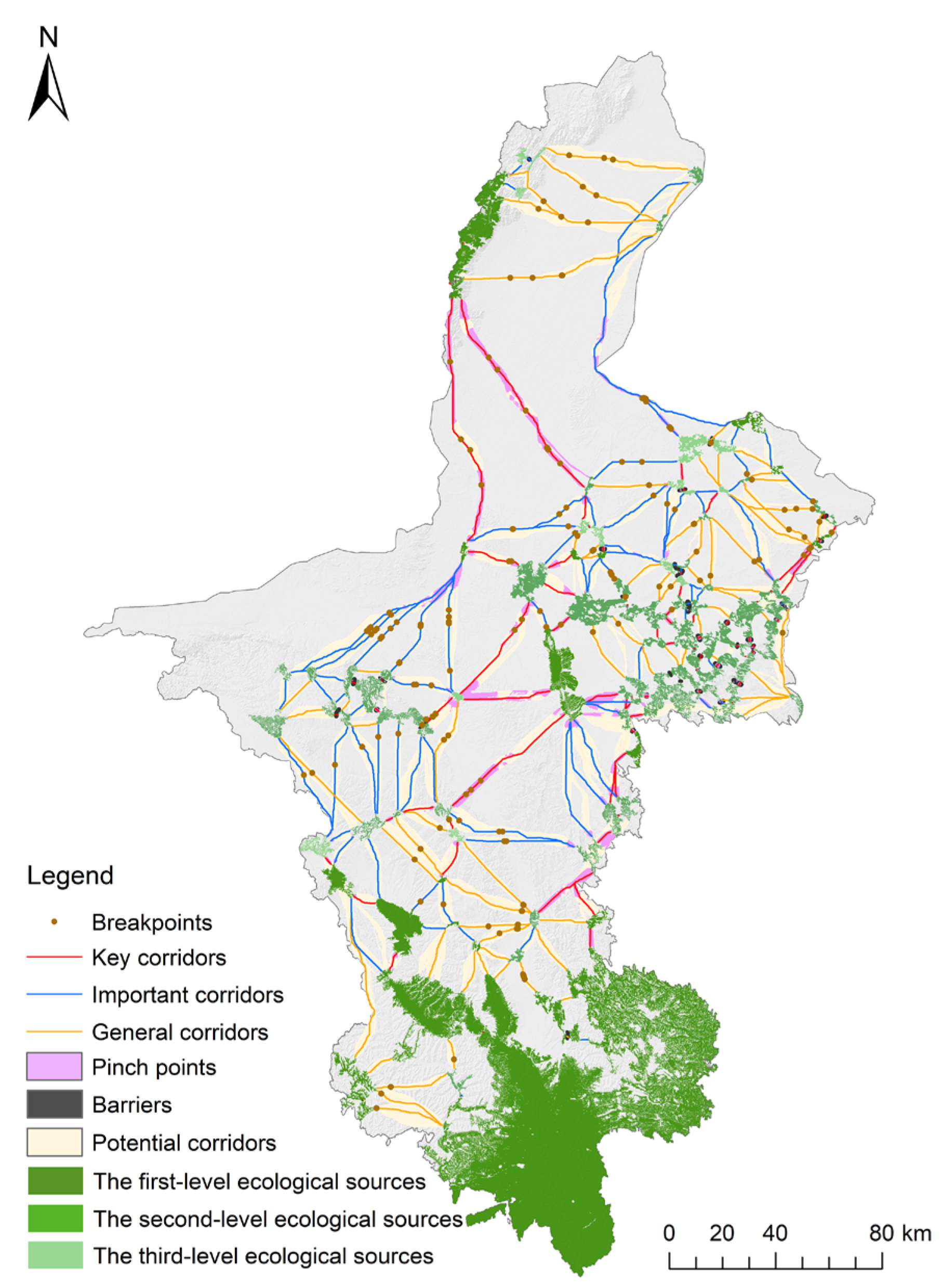
This study identified 4160.67 km of ecological corridors, including 691.45 km of key corridors, 1888.66 km of important corridors, and 1580.56 km of general corridors, and various types of corridors played diverse roles in maintaining stable ecological connectivity across the region. Additionally, the identified 231 ecological pinch points, 45 barriers, and 154 breakpoints were significant for enhancing connectivity and should be prioritized for ecological protection and restoration. The constructed ESP can serve as a key area for preserving regional sustainable landscapes and as a foundation for future optimization of ecological planning.

Overall, the ESP proposed in our study made up for past deficiency of not fully considering the stability of sources in ESP construction. The findings can provide vital insights for policymakers in identifying stable and sustainable priority protection areas and offer valuable scientific and technical support for formulating targeted ecological conservation and restoration strategies in ecologically fragile areas with similar characteristics.

It is worth noting that ecological security involves both ecological and social dimensions. This study primarily concentrated on the ecosystem service supply. However, it is essential to extend further research to incorporate a broader range of key ecological processes and the dynamic changes in the demand for ecosystem services, particularly in the context of increasing attention to human well-being. Additionally, due to limitations in the availability of species data, our study did not consider the specific habitat requirements of certain species and focused solely on the spatial positioning of ecological corridors, neglecting their width. In fact, the width of ecological corridors significantly influences species migration routes [73], and ecological corridors should be designed with ecological considerations regarding their practical significance and widths [2]. Consequently, the next research direction is to investigate the optimal width of ecological corridors by considering the specific migration characteristics of species, the ecological effects of corridors [74], and the impact of changes in landscape patterns and ecosystem functions on these corridors.

References

1. Modica, G.; Praticò, S.; Laudari, L.; Ledda, A.; Di Fazio, S.; De Montis, A. Implementation of multispecies ecological networks at the regional scale: Analysis and multi-temporal assessment. J. Environ. Manag. 2021, 289, 112494. [Google Scholar] [CrossRef] [PubMed]
2. Wei, L.; Zhou, L.; Sun, D.; Yuan, B.; Hu, F. Evaluating the impact of urban expansion on the habitat quality and constructing ecological security patterns: A case study of Jiziwan in the Yellow River Basin, China. Ecol. Indic. 2022, 145, 109544. [Google Scholar] [CrossRef]
3. Peng, J.; Yang, Y.; Liu, Y.; Hu, Y.n.; Du, Y.; Meersmans, J.; Qiu, S. Linking ecosystem services and circuit theory to identify ecological security patterns. Sci. Total Environ. 2018, 644, 781–790. [Google Scholar] [CrossRef] [PubMed]
4. Jia, Q.; Jiao, L.; Lian, X.; Wang, W. Linking supply-demand balance of ecosystem services to identify ecological security patterns in urban agglomerations. Sustain. Cities Soc. 2023, 92, 104497. [Google Scholar] [CrossRef]
5. Ding, M.; Liu, W.; Xiao, L.; Zhong, F.; Lu, N.; Zhang, J.; Zhang, Z.; Xu, X.; Wang, K. Construction and optimization strategy of ecological security pattern in a rapidly urbanizing region: A case study in central-south China. Ecol. Indic. 2022, 136, 108604. [Google Scholar] [CrossRef]
6. Yu, K. Security patterns and surface model in landscape ecological planning. Landsc. Urban Plan. 1996, 36, 1–17. [Google Scholar] [CrossRef]
7. Fan, F.; Liu, Y.; Chen, J.; Dong, J. Scenario-based ecological security patterns to indicate landscape sustainability: A case study on the Qinghai-Tibet Plateau. Landsc. Ecol. 2021, 36, 2175–2188. [Google Scholar] [CrossRef]
8. Peng, J.; Zhao, S.; Dong, J.; Liu, Y.; Meersmans, J.; Li, H.; Wu, J. Applying ant colony algorithm to identify ecological security patterns in megacities. Environ. Model. Softw. 2019, 117, 214–222. [Google Scholar] [CrossRef]
9. Dai, L.; Liu, Y.; Luo, X. Integrating the MCR and DOI models to construct an ecological security network for the urban agglomeration around Poyang Lake, China. Sci. Total Environ. 2021, 754, 141868. [Google Scholar] [CrossRef]
10. Jongman, R.H.G.; Külvik, M.; Kristiansen, I. European ecological networks and greenways. Landsc. Urban Plan. 2004, 68, 305–319. [Google Scholar] [CrossRef]
11. Bennett, A.F. Linkages in the Landscape: The Role of Corridors and Connectivity in Wildlife Conservation; IUCN: Gland, Switzerland; Cambridge, UK, 2003. [Google Scholar]
12. Tzoulas, K.; Korpela, K.; Venn, S.; Yli-Pelkonen, V.; Kaźmierczak, A.; Niemela, J.; James, P. Promoting ecosystem and human health in urban areas using Green Infrastructure: A literature review. Landsc. Urban Plan. 2007, 81, 167–178. [Google Scholar] [CrossRef]
13. Long, Y.; Han, H.; Lai, S.-K.; Mao, Q. Urban growth boundaries of the Beijing Metropolitan Area: Comparison of simulation and artwork. Cities 2013, 31, 337–348. [Google Scholar] [CrossRef]
14. Chen, W.; Zhao, H.; Li, J.; Zhu, L.; Wang, Z.; Zeng, J. Land use transitions and the associated impacts on ecosystem services in the Middle Reaches of the Yangtze River Economic Belt in China based on the geo-informatic Tupu method. Sci. Total Environ. 2020, 701, 134690. [Google Scholar] [CrossRef] [PubMed]
15. Gou, M.; Li, L.; Ouyang, S.; Shu, C.; Xiao, W.; Wang, N.; Hu, J.; Liu, C. Integrating ecosystem service trade-offs and rocky desertification into ecological security pattern construction in the Daning river basin of southwest China. Ecol. Indic. 2022, 138, 108845. [Google Scholar] [CrossRef]
16. Wei, H.; Zhu, H.; Chen, J.; Jiao, H.; Li, P.; Xiong, L. Construction and Optimization of Ecological Security Pattern in the Loess Plateau of China Based on the Minimum Cumulative Resistance (MCR) Model. Remote Sens. 2022, 14, 5906. [Google Scholar] [CrossRef]
17. Aminzadeh, B.; Khansefid, M. A case study of urban ecological networks and a sustainable city: Tehran’s metropolitan area. Urban Ecosyst. 2010, 13, 23–36. [Google Scholar] [CrossRef]
18. Yang, Z.; Ma, C.; Liu, Y.; Zhao, H.; Hua, Y.; Ou, S.; Fan, X. Provincial-Scale Research on the Eco-Security Structure in the Form of an Ecological Network of the Upper Yellow River: A Case Study of the Ningxia Hui Autonomous Region. Land 2023, 12, 1341. [Google Scholar] [CrossRef]
19. Xu, W.; Wang, J.; Zhang, M.; Li, S. Construction of landscape ecological network based on landscape ecological risk assessment in a large-scale opencast coal mine area. J. Clean. Prod. 2021, 286, 125523. [Google Scholar] [CrossRef]
20. Li, H.; Chen, H.; Wu, M.; Zhou, K.; Zhang, X.; Liu, Z. A Dynamic Evaluation Method of Urban Ecological Networks Combining Graphab and the FLUS Model. Land 2022, 11, 2297. [Google Scholar] [CrossRef]
21. Li, L.; Huang, X.; Wu, D.; Wang, Z.; Yang, H. Optimization of ecological security patterns considering both natural and social disturbances in China’s largest urban agglomeration. Ecol. Eng. 2022, 180, 106647. [Google Scholar] [CrossRef]
22. Huang, L.; Wang, J.; Fang, Y.; Zhai, T.; Cheng, H. An integrated approach towards spatial identification of restored and conserved priority areas of ecological network for implementation planning in metropolitan region. Sustain. Cities Soc. 2021, 69, 102865. [Google Scholar] [CrossRef]
23. Wang, Z.; Luo, K.; Zhao, Y.; Lechner, A.M.; Wu, J.; Zhu, Q.; Sha, W.; Wang, Y. Modelling regional ecological security pattern and restoration priorities after long-term intensive open-pit coal mining. Sci. Total Environ. 2022, 835, 155491. [Google Scholar] [CrossRef] [PubMed]
24. Shen, Z.; Wu, W.; Chen, S.; Tian, S.; Wang, J.; Li, L. A static and dynamic coupling approach for maintaining ecological networks connectivity in rapid urbanization contexts. J. Clean. Prod. 2022, 369, 133375. [Google Scholar] [CrossRef]
25. Nie, W.; Xu, B.; Yang, F.; Shi, Y.; Liu, B.; Wu, R.; Lin, W.; Pei, H.; Bao, Z. Simulating future land use by coupling ecological security patterns and multiple scenarios. Sci. Total Environ. 2023, 859, 160262. [Google Scholar] [CrossRef]
26. Nie, W.; Shi, Y.; Siaw, M.J.; Yang, F.; Wu, R.; Wu, X.; Zheng, X.; Bao, Z. Constructing and optimizing ecological network at county and town Scale: The case of Anji County, China. Ecol. Indic. 2021, 132, 108294. [Google Scholar] [CrossRef]
27. Knaapen, J.P.; Scheffer, M.; Harms, B. Estimating habitat isolation in landscape planning. Landsc. Urban Plan. 1992, 23, 1–16. [Google Scholar] [CrossRef]
28. McRae, B.H.; Dickson, B.G.; Keitt, T.H.; Shah, V.B. Using circuit theory to model connectivity in ecology, evolution, and conservation. Ecology 2008, 89, 2712–2724. [Google Scholar] [CrossRef] [PubMed]
29. Zhang, Y.; Zhao, Z.; Fu, B.; Ma, R.; Yang, Y.; Lü, Y.; Wu, X. Identifying ecological security patterns based on the supply, demand and sensitivity of ecosystem service: A case study in the Yellow River Basin, China. J. Environ. Manag. 2022, 315, 115158. [Google Scholar] [CrossRef]
30. Liu, H.; Niu, T.; Yu, Q.; Yang, L.; Ma, J.; Qiu, S.; Wang, R.; Liu, W.; Li, J. Spatial and temporal variations in the relationship between the topological structure of eco-spatial network and biodiversity maintenance function in China. Ecol. Indic. 2022, 139, 108919. [Google Scholar] [CrossRef]
31. Zeng, W.; Tang, H.; Liang, X.; Hu, Z.; Yang, Z.; Guan, Q. Using ecological security pattern to identify priority protected areas: A case study in the Wuhan Metropolitan Area, China. Ecol. Indic. 2023, 148, 110121. [Google Scholar] [CrossRef]
32. Lyu, R.; Clarke, K.C.; Zhang, J.; Feng, J.; Jia, X.; Li, J. Spatial correlations among ecosystem services and their socio-ecological driving factors: A case study in the city belt along the Yellow River in Ningxia, China. Appl. Geogr. 2019, 108, 64–73. [Google Scholar] [CrossRef]
33. Snäll, T.; Triviño, M.; Mair, L.; Bengtsson, J.; Moen, J. High rates of short-term dynamics of forest ecosystem services. Nat. Sustain. 2021, 4, 951–957. [Google Scholar] [CrossRef]
34. Lü, D.; Lü, Y.; Gao, G.; Sun, S.; Wang, Y.; Fu, B. A landscape persistence-based methodological framework for assessing ecological stability. Environ. Sci. Ecotechnol. 2024, 17, 100300. [Google Scholar] [CrossRef]
35. Jóźwik, J.; Dymek, D. Spatial diversity of ecological stability in different types of spatial units: Case study of Poland. Acta Geogr. Slov. 2021, 61, 57–74. [Google Scholar] [CrossRef]
36. Guilherme, F.; Gonçalves, J.A.; Carretero, M.A.; Farinha-Marques, P. Assessment of land cover trajectories as an indicator of urban habitat temporal continuity. Landsc. Urban Plan. 2024, 242, 104932. [Google Scholar] [CrossRef]
37. Ji, X.; Wu, D.; Yan, Y.; Guo, W.; Li, K. Interpreting regional ecological security from perspective of ecological networks: A case study in Ningxia Hui Autonomous Region, China. Environ. Sci. Pollut. Res. 2023, 30, 65412–65426. [Google Scholar] [CrossRef]
38. Xu, J.; Wang, S.; Xiao, Y.; Xie, G.; Wang, Y.; Zhang, C.; Li, P.; Lei, G. Mapping the spatiotemporal heterogeneity of ecosystem service relationships and bundles in Ningxia, China. J. Clean. Prod. 2021, 294, 126216. [Google Scholar] [CrossRef]
39. Du, L.; Gong, F.; Zeng, Y.; Ma, L.; Qiao, C.; Wu, H. Carbon use efficiency of terrestrial ecosystems in desert/grassland biome transition zone: A case in Ningxia province, northwest China. Ecol. Indic. 2021, 120, 106971. [Google Scholar] [CrossRef]
40. Dong, J.; Zhou, Y.; You, N. A 30-m Annual Maximum NDVI Dataset in China from 2000 to 2020. 2021. Available online: http://www.nesdc.org.cn/sdo/detail?id=60f68d757e28174f0e7d8d49 (accessed on 26 December 2023).
41. Peng, S. 1-km Monthly Precipitation Dataset for China (1901–2022). 2020. Available online: http://loess.geodata.cn/data/datadetails.html?dataguid=192891852410344&docid=490 (accessed on 26 December 2023).
42. Peng, S. 1 km Monthly Potential Evapotranspiration Dataset in China (1901–2022). 2022. Available online: http://loess.geodata.cn/data/datadetails.html?dataguid=34595274939620&docid=74 (accessed on 26 December 2023).
43. Van Meerbeek, K.; Jucker, T.; Svenning, J.-C. Unifying the concepts of stability and resilience in ecology. J. Ecol. 2021, 109, 3114–3132. [Google Scholar] [CrossRef]
44. Saura, S.; Torné, J. Conefor Sensinode 2.2: A software package for quantifying the importance of habitat patches for landscape connectivity. Environ. Model. Softw. 2009, 24, 135–139. [Google Scholar] [CrossRef]
45. Feng, Z.; Jin, X.; Chen, T.; Wu, J. Understanding trade-offs and synergies of ecosystem services to support the decision-making in the Beijing–Tianjin–Hebei region. Land Use Pol. 2021, 106, 105446. [Google Scholar] [CrossRef]
46. Xia, H.; Yuan, S.; Prishchepov, A.V. Spatial-temporal heterogeneity of ecosystem service interactions and their social-ecological drivers: Implications for spatial planning and management. Resour. Conserv. Recycl. 2023, 189, 106767. [Google Scholar] [CrossRef]
47. Natural Capital Project. InVEST 3.14.1 User’s Guide. The Natural Capital Project. Stanford University, University of Minnesota, Chinese Academy of Sciences, The Nature Conservancy, World Wildlife Fund, Stockholm Resilience Centre and the Royal Swedish Academy of Sciences. Available online: https://naturalcapitalproject.stanford.edu/software/invest (accessed on 7 May 2003).
48. Benavidez, R.; Jackson, B.; Maxwell, D.; Norton, K. A review of the (Revised) Universal Soil Loss Equation ((R)USLE): With a view to increasing its global applicability and improving soil loss estimates. Hydrol. Earth Syst. Sci. 2018, 22, 6059–6086. [Google Scholar] [CrossRef]
49. Guo, Z.; Xie, Y.; Guo, H.; Zhang, X.; Wang, H.; Bie, Q.; Xi, G.; Ma, C. Do the ecosystems of Gansu Province in Western China’s crucial ecological security barrier remain vulnerable? Evidence from remote sensing based on geospatial analysis. J. Clean. Prod. 2023, 402, 136740. [Google Scholar] [CrossRef]
50. Jiang, H.; Peng, J.; Dong, J.; Zhang, Z.; Xu, Z.; Meersmans, J. Linking ecological background and demand to identify ecological security patterns across the Guangdong-Hong Kong-Macao Greater Bay Area in China. Landsc. Ecol. 2021, 36, 2135–2150. [Google Scholar] [CrossRef]
51. Taylor, P.D.; Fahrig, L.; Henein, K.; Merriam, G. Connectivity Is a Vital Element of Landscape Structure. Oikos 1993, 68, 571. [Google Scholar] [CrossRef]
52. Zhang, L.; Peng, J.; Liu, Y.; Wu, J. Coupling ecosystem services supply and human ecological demand to identify landscape ecological security pattern: A case study in Beijing–Tianjin–Hebei region, China. Urban Ecosyst. 2017, 20, 701–714. [Google Scholar] [CrossRef]
53. Pascual-Hortal, L.; Saura, S. Comparison and development of new graph-based landscape connectivity indices: Towards the priorization of habitat patches and corridors for conservation. Landsc. Ecol. 2006, 21, 959–967. [Google Scholar] [CrossRef]
54. Carranza, M.L.; D’Alessandro, E.; Saura, S.; Loy, A. Connectivity providers for semi-aquatic vertebrates: The case of the endangered otter in Italy. Landsc. Ecol. 2012, 27, 281–290. [Google Scholar] [CrossRef]
55. Saura, S.; Pascual-Hortal, L. A new habitat availability index to integrate connectivity in landscape conservation planning: Comparison with existing indices and application to a case study. Landsc. Urban Plan. 2007, 83, 91–103. [Google Scholar] [CrossRef]
56. Yu, H.; Huang, J.; Ji, C.; Li, Z.A. Construction of a Landscape Ecological Network for a Large-Scale Energy and Chemical Industrial Base: A Case Study of Ningdong, China. Land 2021, 10, 344. [Google Scholar] [CrossRef]
57. Xie, J.; Xie, B.; Zhou, K.; Li, J.; Xiao, J.; Liu, C.; Zhang, X. Multiple Probability Ecological Network and County-Scale Management. Land 2023, 12, 1600. [Google Scholar] [CrossRef]
58. Lu, Z.; Li, W.; Zhou, S. Constructing a resilient ecological network by considering source stability in the largest Chinese urban agglomeration. J. Environ. Manag. 2023, 328, 116989. [Google Scholar] [CrossRef]
59. Liu, C.; Wu, X.; Wang, L. Analysis on land ecological security change and affect factors using RS and GWR in the Danjiangkou Reservoir area. China. Appl. Geogr. 2019, 105, 1–14. [Google Scholar] [CrossRef]
60. Keeley, A.T.H.; Beier, P.; Keeley, B.W.; Fagan, M.E. Habitat suitability is a poor proxy for landscape connectivity during dispersal and mating movements. Landsc. Urban Plan. 2017, 161, 90–102. [Google Scholar] [CrossRef]
61. Li, L.; Hu, R.; Huang, J.; Bürgi, M.; Zhu, Z.; Zhong, J.; Lü, Z. A farmland biodiversity strategy is needed for China. Nat. Ecol. Evol. 2020, 4, 772–774. [Google Scholar] [CrossRef]
62. Li, H.; Zhang, T.; Cao, X.-S.; Zhang, Q.-Q. Establishing and Optimizing the Ecological Security Pattern in Shaanxi Province (China) for Ecological Restoration of Land Space. Forests 2022, 13, 766. [Google Scholar] [CrossRef]
63. Liu, Y.; Lü, Y.; Fu, B.; Harris, P.; Wu, L. Quantifying the spatio-temporal drivers of planned vegetation restoration on ecosystem services at a regional scale. Sci. Total Environ. 2019, 650, 1029–1040. [Google Scholar] [CrossRef]
64. Wang, S.; Wu, M.; Hu, M.; Xia, B. Integrating ecosystem services and landscape connectivity into the optimization of ecological security pattern: A case study of the Pearl River Delta, China. Environ. Sci. Pollut. Res. 2022, 29, 76051–76065. [Google Scholar] [CrossRef]
65. Miu, I.V.; Rozylowicz, L.; Popescu, V.D.; Anastasiu, P. Identification of areas of very high biodiversity value to achieve the EU Biodiversity Strategy for 2030 key commitments. PeerJ 2020, 8, e10067. [Google Scholar] [CrossRef]
66. Timmers, R.; Van Kuijk, M.; Verweij, P.A.; Ghazoul, J.; Hautier, Y.; Laurance, W.F.; Arriaga-Weiss, S.L.; Askins, R.A.; Battisti, C.; Berg, Å.; et al. Conservation of birds in fragmented landscapes requires protected areas. Front. Ecol. Environ. 2022, 20, 361–369. [Google Scholar] [CrossRef]
67. Shrestha, N.; Xu, X.; Meng, J.; Wang, Z. Vulnerabilities of protected lands in the face of climate and human footprint changes. Nat. Commun. 2021, 12, 1632. [Google Scholar] [CrossRef] [PubMed]
68. Ghoddousi, A.; Loos, J.; Kuemmerle, T. An Outcome-Oriented, Social–Ecological Framework for Assessing Protected Area Effectiveness. Bioscience 2021, 72, 201–212. [Google Scholar] [CrossRef] [PubMed]
69. Myers, N.; Mittermeier, R.A.; Mittermeier, C.G.; Da Fonseca, G.A.; Kent, J. Biodiversity hotspots for conservation priorities. Nature 2000, 403, 853–858. [Google Scholar] [CrossRef] [PubMed]
70. Li, L.; Huang, X.; Wu, D.; Yang, H. Construction of ecological security pattern adapting to future land use change in Pearl River Delta. China. Appl. Geogr. 2023, 154, 102946. [Google Scholar] [CrossRef]
71. The General Office of the People’s Government of Ningxia Hui Autonomous Region. The 14th Five-Year Plan for the Protection and Utilization of Natural Resources in Ningxia Hui Autonomous Region. Available online: https://www.nx.gov.cn/zwgk/qzfwj/202109/t20210924_3045970.html (accessed on 25 September 2023).
72. Dominguez, J.C.; Calero-Riestra, M.; Olea, P.P.; Malo, J.E.; Burridge, C.P.; Proft, K.; Illanas, S.; Viñuela, J.; García, J.T. Lack of detectable genetic isolation in the cyclic rodent Microtus arvalis despite large landscape fragmentation owing to transportation infrastructures. Sci. Rep. 2021, 11, 12534. [Google Scholar] [CrossRef]
73. Lindenmayer, D.B.; Nix, H.A. Ecological Principles for the Design of Wildlife Corridors. Conserv. Biol. 1993, 7, 627–631. [Google Scholar] [CrossRef]
74. Fahrig, L. Effects of Habitat Fragmentation on Biodiversity. Annu. Rev. Ecol. Evol. Syst. 2003, 34, 487–515. [Google Scholar] [CrossRef]
Figure 1. The location of Ningxia Hui Autonomous Region (NHAR); (a) geographical location of the study area (produced based on the standard map with reference number GS (2019)1708); (b) elevation; and (c) land use maps of the years 2000, 2010, and 2020.
Land 13 00214 g001
Figure 2. Methodological framework for constructing the ESP in NHAR.
Land 13 00214 g002
Figure 3. Process of identifying ecological sources considering stability.
Land 13 00214 g003
Figure 4. Spatial–temporal distribution of ecosystem services in NHAR.
Land 13 00214 g004
Figure 5. Spatial distribution of the ESI in NHAR for the years 2000, 2010, and 2020.
Land 13 00214 g005
Figure 6. The overall change patterns of the ESI and the area proportion of various pattern types.
Land 13 00214 g006
Figure 7. Spatial distribution of stable ecological sources and the area proportion of three levels of sources.
Land 13 00214 g007
Figure 8. Composition and proportions of land use types in stable ecological sources for the years 2000, 2010, and 2020.
Land 13 00214 g008
Figure 9. Ecological resistance factors and comprehensive ecological resistance surface in NHAR.
Land 13 00214 g009
Figure 10. The ESP construction in NHAR.
Land 13 00214 g010