County-Level Land Use Carbon Budget in the Yangtze River Economic Belt, China: Spatiotemporal Differentiation and Coordination Zoning

Abstract

The local land use carbon budget (LUCB) balance is an important factor in achieving regional carbon neutrality. As the basic unit of China’s economic development and social governance, the county level is an important part of the realization of the “double carbon” goal. This paper focuses on 1069 county units within the Yangtze River Economic Belt (YREB). It utilizes data on land use, nighttime light, energy consumption, and social and economic factors to construct carbon emission models. The spatiotemporal characteristics of LUCB in these county units are analyzed using standard deviational ellipse (SDE) and spatial autocorrelation methods. Additionally, a zoning study is conducted by examining the economic contribution coefficient (ECC) of carbon emissions, the ecological support coefficient (ESC), and their coupling relationship. The results show that (1) the total land use carbon emissions (LUCE) increased significantly during the research period, and the total carbon sink was relatively stable. (2) The LUCB is spatially high in the east and low in the west, with the center of gravity moving to the southwest as a whole. (3) The LUCB shows positive spatial autocorrelation and has significant spatial agglomeration characteristics, which are mainly high–high and low–low regional agglomeration types. (4) The ECC is high in the east and low in the west, the ESC is high in the west and low in the east, and the coordination and coupling degrees of the two are low. (5) According to the ECC and ESC, the county unit is divided into a low-carbon conservation area, an economic development area, a carbon sink development area, and a comprehensive optimization area. This study is helpful in promoting the sustainable development of carbon neutrality and low carbon in the YREB.

1. Introduction

In response to the challenge of global warming, the main cause of which is carbon emissions caused by human activities, 197 countries have adopted policies to target net zero emissions [1]. In September 2020, the Chinese government put forward the strategic goal of reaching its carbon peak by 2030 and achieving carbon neutrality by 2060 [2,3]. As the carrier of human production, life, and the terrestrial ecosystem, land has dual attributes. On the one hand, land use constitutes the primary contributor to carbon emissions, making up 27% of the overall human emissions [4]. On the other hand, land use is closely related to carbon sink [5], mainly absorbing carbon dioxide from the air for vegetation photosynthesis [6]. Studies have shown that global terrestrial ecosystems (woodlands, grasslands) absorbed 31% of the carbon emissions from human activities during 2010–2019 [7]. The land use carbon budget (LUCB) is the sum of carbon emissions and carbon sinks under different land use modes, so it is of great significance to study the LUCB to promote regional carbon neutrality.

Scholars have conducted a lot of research on the LUCB, mainly focusing on the calculation of the LUCB, spatial distribution characteristics, research scale, and influencing factors. In the calculation and research of the LUCB, scholars mainly use the Bookkeeping Model [8,9,10], Sample site inventory method [11,12], and the IPCC emission factor method [4,13,14]. In terms of the research on the spatial distribution characteristics of land use carbon emissions (LUCEs), scholars have studied the spatial characteristics of different types of LUCE and found that different types of land use show obvious spatial differences in terms of carbon budget. For example, woodlands [15] and grasslands [16] are the main contributors to carbon sinks, while construction land [17] and industrial land [18] are the main contributors to carbon emissions. In terms of the research scale of the LUCB, scholars have mainly studied the global [19,20], national [21,22], and urban [23] scales. In studies on the influencing factors of the LUCB, Log-mean partition index (LMDI) [24], IPAT model [25], population, affluence, and the technology regression random influence model (STIRPAT) [26] are often used. There is little research on the coordination zoning of the carbon budget. At present, carbon balance zoning is mainly based on the economic contribution coefficient (ECC) and ecological support coefficient (ESC).

While scholars have extensively studied LUCE, there are still some deficiencies. Energy consumption data are often the main basis for the indirect calculation of carbon emissions from construction land. However, China’s energy consumption data are relatively complete at the provincial level, while there are serious deficiencies at the county level [27]. Therefore, there are few studies on carbon emissions from land use at the county level. However, the county level is the basic spatial unit and carrier of China’s economic development and industrial transfer [28], which is of great significance for China to achieve the goal of “dual carbon”. Therefore, it is urgent to study LUCE at the county level. With the progress of remote sensing technology, studies have found that there is a significant correlation between nighttime light intensity and energy consumption carbon emissions, and the data on energy carbon emissions can be retrieved on a smaller scale with the help of nighttime light data [9].

The YREB plays a vital role in China’s economic development. In November 2018, the CPC Central Committee and the State Council emphasized that the Yangtze River Economic Belt (YREB) should utilize its geographical advantages [29]. It should focus on common protection, avoid large-scale development, prioritize ecology and green development, and rely on the Yangtze River as a golden waterway [30]. The goal is to promote coordinated development in the upper, middle, and lower reaches of the Yangtze River, along with high-quality development along the river. However, there are still many difficulties in the construction of ecological civilization and the road to green development in the YREB. Rapid economic development has intensified the expansion of construction, accelerated the loss of high-quality cropland and ecological land, and caused a large amount of carbon emissions [31]. Based on this, this paper takes 1069 county units in the YREB as its research object and uses land use data, nighttime light data, energy consumption data, and social and economic data to build carbon emission models and analyze the spatiotemporal characteristics of the carbon budget of county units in the YREB by using standard deviational ellipse (SDE) and spatial autocorrelation methods. Then, by analyzing the ECC, the ESC, and the coupling relationship between the two, this paper conducts a zoning study, and on this basis, puts forward policy suggestions for the future development of various zoning units in order to provide a basis for the low-carbon development of the YREB.

2. Study Area and Data Source

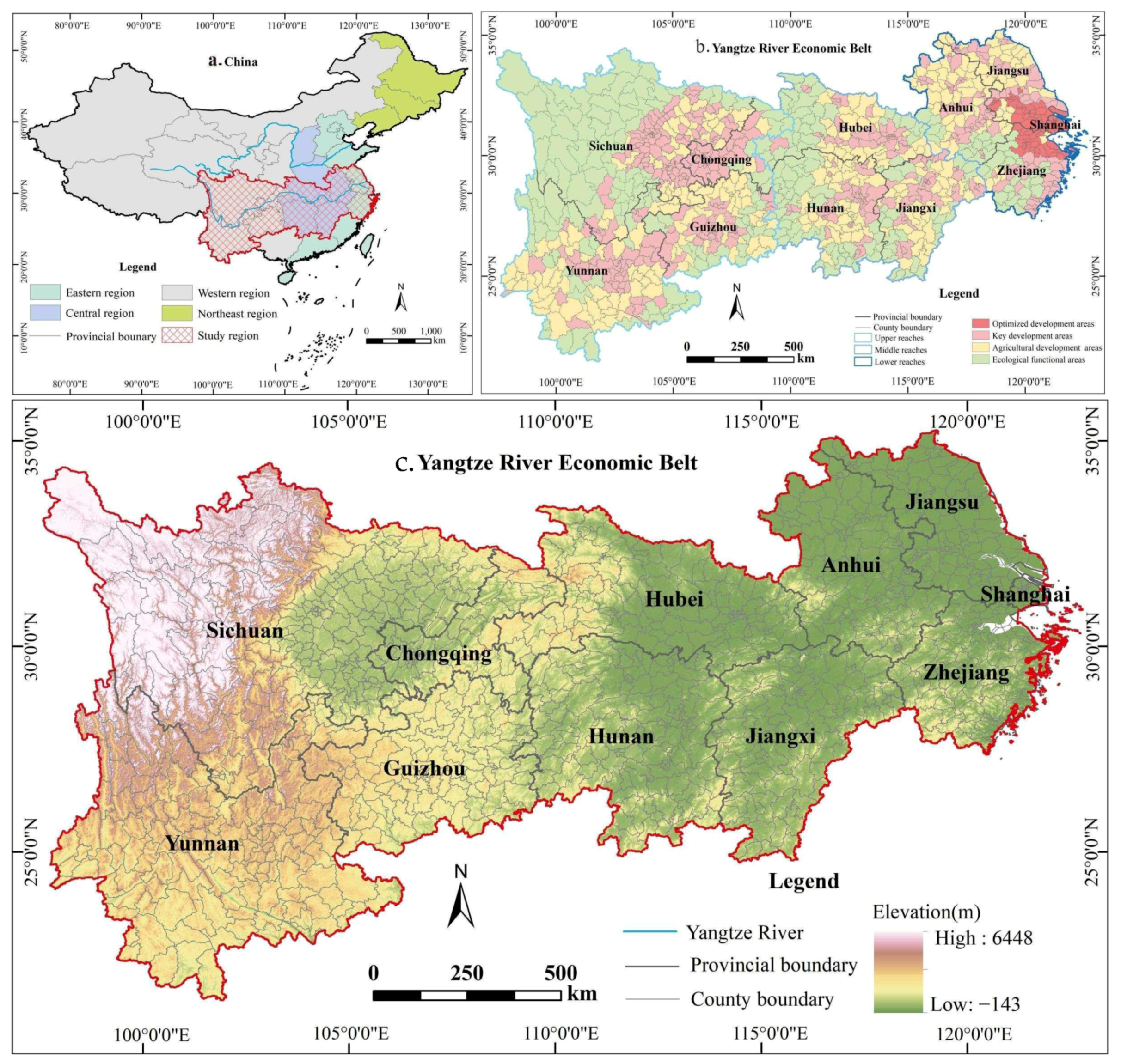
2.1. Overview of the Study Area

The YREB (Figure 1) stands as a preeminent economic powerhouse within the Chinese territorial landscape, representing a focal point of national developmental aspirations. It spans the vast expanse of the country’s western, central, and eastern regions, encompassing the provinces and municipalities of Sichuan, Guizhou, Yunnan, Hunan, Hubei, Jiangxi, Anhui, Zhejiang, Jiangsu, Shanghai, and Chongqing, collectively encompassing a landmass of roughly 2.05 million square kilometers. Within this expansive region, Shanghai, Zhejiang, Jiangsu, and Anhui constitute the lower reaches of the Yangtze River, while Jiangxi, Hubei, and Hunan form the middle reaches, and Chongqing, Guizhou, Sichuan, and Yunnan comprise the upper reaches.

2.2. Data Sources

Land use data were procured from the Landsat TM image interpretation data (https://www.resdc.cn/, accessed on 1 January 2022). Following the classification methodology outlined by esteemed predecessors [32], the categorization of land use types encompasses cropland, woodland, grassland, water, construction land, and unused land, amounting to a comprehensive suite of six distinct types. The energy data come from the balance table of terminal energy consumption in the China Energy Statistical Yearbook (2001–2021). The nighttime light data are derived from the Chinese long-time series night light dataset (2000–2020) corrected by Xiao (2022). The social and economic data mainly come from the 2021 China County Statistical Yearbook and the Statistical Bulletin of National Economic and Social Development of each district and county.

2.3. Calculation and Research Methods

2.3.1. Approach for Computing LUCB

Methodology for Calculating Carbon Emissions Directly

The carbon emission model is as follows:

$${{\rm E}}_{\kappa }={\displaystyle \sum E_i}={\displaystyle \sum T_i}\times {\delta }_i\times 44/12$$

(1)

where E_k represents the direct carbon emissions; E_i denotes the carbon emissions generated within the ith land use type; T_i corresponds to the area of the ith land use type; δ_i is the carbon emission (absorption) coefficient for the ith land use type; and “44/12” is utilized to transform the mass of carbon into a mass of carbon dioxide. Drawing upon the insights of previous research [33,34], the established carbon emission (absorption) coefficients for cropland, woodland, grassland, water, and unused land are determined as 0.422 t/ha².a −0.644 t/ha².a, −0.021 t/ha².a, −0.253 t/ha².a, and −0.005 t/ha².a, respectively.

2.3.2. Methodology for Calculating Indirect Carbon Emissions

The carbon emissions from construction land are indirectly calculated based on energy consumption data. In this context, we utilize the terminal energy consumption data from the China Energy Statistical Yearbook, excluding energy consumption in agriculture, forestry, animal husbandry, fisheries, and water conservancy. The specific types of energy include raw coal, washed anthracite, other washed coal, shaped coal, coke, other coking products, coke oven gas, blast furnace gas, other gases, natural gas, crude oil, gasoline, kerosene, diesel, fuel oil, liquefied petroleum gas, refinery dry gas, other petroleum products, electricity, and heat. The calculation of carbon emissions from fossil energy sources follows the referenced formula outlined below:

$$E_1={\displaystyle {\sum }_{i=1}^{18}{e}_i\times {cef}_i}$$

(2)

$${cef}_i=c{c}_i\times nc{v}_i\times o_i\times 44/12$$

(3)

where E₁ represents the carbon emissions resulting from the consumption of fossil energy, and e_i denotes various types of energy. The variables cef_i, cc_i, ncv_i, and o_i signify the carbon emission factor, carbon content per unit heat value, net calorific value, and carbon oxidation rate for different energy types, respectively. The values for carbon content per unit heat value and carbon oxidation rate are sourced from the “Provincial Greenhouse Gas Inventory Compilation Guidelines”. The lower heating value of fossil energy is derived from the “China Energy Statistical Yearbook”.

The carbon emissions resulting from electricity and heat, denoted as E₂, are computed utilizing the methodology proposed by previous research [35].

$$E=E_1+E_2$$

(4)

where E stands for total energy consumption emissions.

Based on the night light data, the carbon emissions of energy consumption at the provincial level were inverted to the county level according to the top-down decomposition method of predecessors [36]. It is assumed that there is a linear relationship between the Digital Number (DN) value of night light brightness and energy carbon emissions, and the higher the DN value, the larger the carbon emissions, and this hypothesis has a consistent relationship at the provincial and county scales. The estimation model is as follows:

$$C{E}_i=a\times TN{L}_i+\theta$$

(5)

where CE_i is the carbon emission of province i; TNL_i is the total DN value of province i; a is the regression coefficient, and θ represents the error value.

In order to reduce heteroscedasticity fluctuations, logarithmic processing of the two variables is performed, and the formula is as follows:

$$LnC{E}_i=a_{i}LnTN{L}_i+{\beta }_i+\theta$$

(6)

where a_i represents the regression coefficient of each province; β_i represents a fixed coefficient for each province; and θ represents the error value.

According to the above series of tests, the carbon emission model is as follows:

LnCE_it = a_iLnTNL_it + β_i + 0.5595 I = 1, 2, …, 11; t = 2000, 2001, …, 2020

(7)

AdjR² = 0.9058 F-stat = 106.3944 F.prob = 0.0000

where CE_it represents the energy consumption carbon emissions of province i in year t, TNL_it represents the DN value of province i in year t, regression coefficient a and fixed coefficient β change with the change in i of the specific province, and AdjR² is an evaluation metric in regression analysis used to assess the goodness of fit of a model to observed data. This shows that the remote sensing data of night light can explain the carbon emission of energy consumption very significantly. According to the regression coefficient and fixed coefficient of each province, the energy carbon emission of the corresponding province is obtained based on the nighttime light data. This work compares each province’s statistics on energy carbon emissions with the predicted values using Lv’s study methodology (2020) in an effort to further confirm the accuracy of the estimated energy carbon emissions of each province. The average error is 10.41%, and the fitting coefficient of the two is R² = 0.92, which meets the accuracy requirements. A top-down model is used to estimate carbon emissions from energy consumption at the county level, as follows:

$$C_c=C_i\times (C{E}_c/C{E}_i)$$

(8)

where C_c represents the adjusted energy carbon emissions of a particular county; C_i represents the statistical value of energy carbon emissions in a specific province; CE_c represents an estimate of energy carbon emissions for a particular county; and CE_i represents estimates of energy carbon emissions for a particular province.

2.4. Research Methods

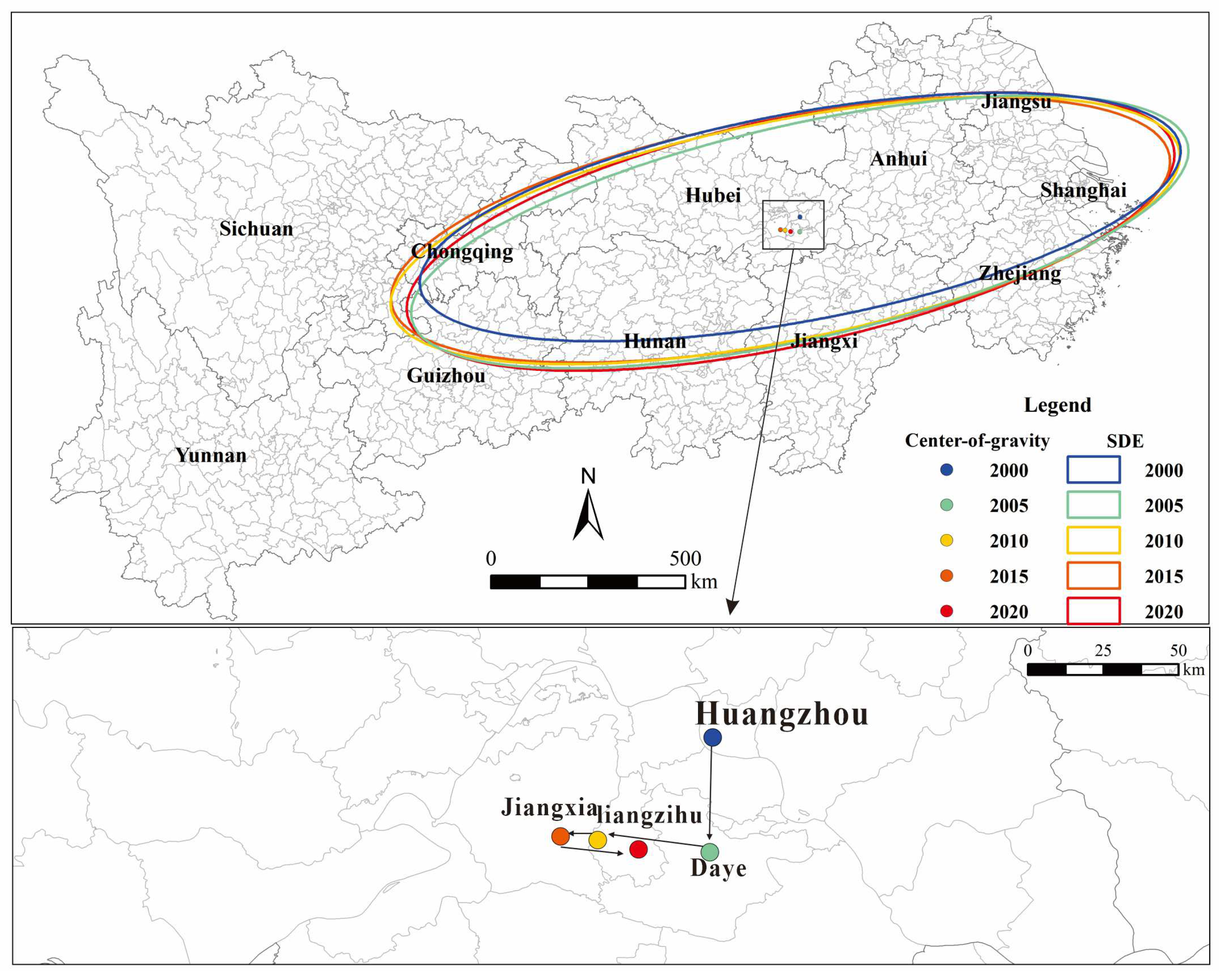
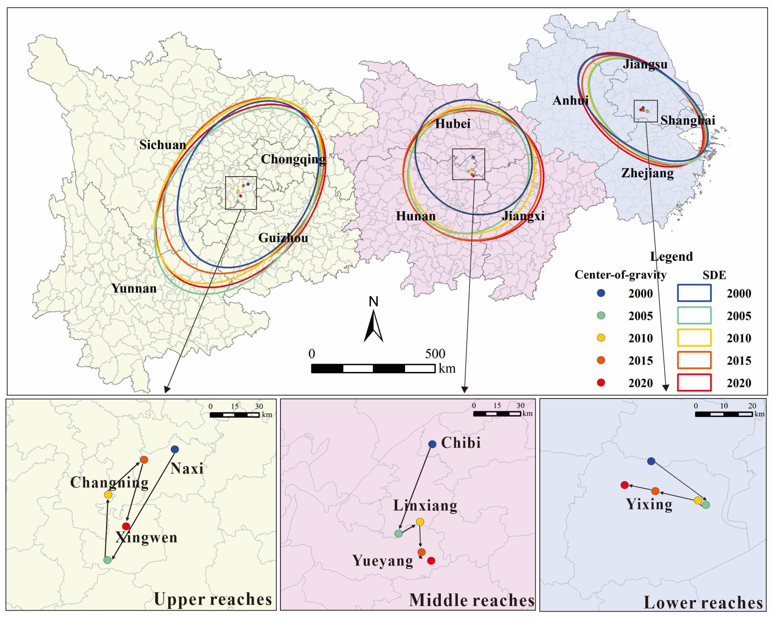
2.4.1. Standard Deviational Ellipse Analysis Method

Standard deviation ellipse (SDE) is a spatial statistical technique to measure the distribution pattern of geographical elements. The spatiotemporal distribution characteristics of LUCB at the county level in China can be analyzed through the parameters of the center of gravity, angle θ, X-axis, and Y-axis standard difference. The long axis of the ellipse symbolizes the principal orientation of the dataset distribution, while its area signifies the level of concentration (dispersion) within the dataset distribution [37]. The specific formula is as follows:

$$\overline{X}=\frac{1}{n}{\displaystyle \sum _{i=1}^n{x}_i}, \overline{Y}=\frac{1}{n}{\displaystyle \sum _{i=1}^n{y}_i}$$

(9)

where $\overline{X}$ and $\overline{Y}$ represents the center-of-gravity coordinates; $x_i$ and $y_i$ represent the coordinates of each administrative unit’s center in this study area; and n signifies the total number of counties.

2.4.2. Global Spatial Autocorrelation Analysis

Global spatial autocorrelation uses Moran’s global index, which is expressed as follows [38]:

$$I=\frac{n{\displaystyle {\sum }_{i=1}^n{\displaystyle {\sum }_{j=1}^n{w}_{ij}\left(xi-\overline{x}\right)\left(xj-\overline{x}\right)}}}{{\displaystyle {\sum }_{i=1}^n{\displaystyle {\sum }_{j=1}^n{w}_{ij}{\displaystyle {\sum }_{i=1}^n{\left(xi-\overline{x}\right)}^2}}}}$$

(10)

where I is Moran’s global index value; n represents the number of research objects; x_i and x_j are the observed values of the target genus characteristics in the study object i and j; w_ij is the adjacent weight of objects i and j; and $\bar{x}$ represents the mean value of the attribute pertaining to the research object.

$$Z(I)=\frac{I-E(I)}{\sqrt{VAR\left(I\right)}}$$

(11)

where the Z(I) value is computed for hypothesis testing to assess whether there is a significant spatial autocorrelation among the observed values; E(I) and Var(I) represent the mean value and variance of I, respectively.

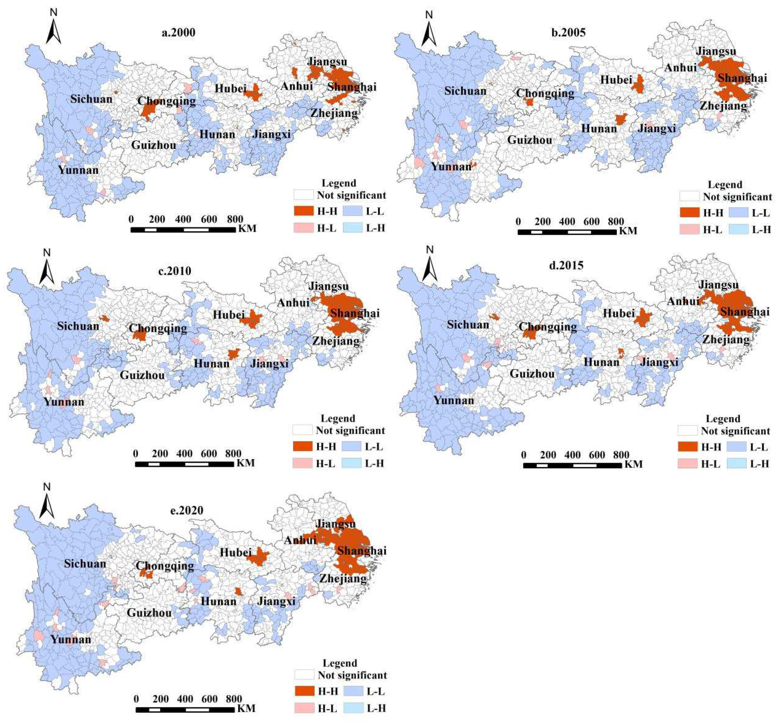
2.4.3. Local Spatial Autocorrelation Analysis

Local spatial autocorrelation (LISA) can effectively reveal the agglomeration of elements at specific locations in the study area, and the LISA index can decompose Moran’s global I into each part of the entire spatial range. The expression is as follows [39]:

$$I_i=x_i^{’}{\displaystyle \sum _{j=1}^n{w}_{ij}}{x}_j^{’}$$

(12)

where I_i is Moran’s local index; x’_i and x’_j are standardized unit observations; and w_ij is the weight.

2.4.4. ECC-The Economic Contribution Coefficient of Carbon Emission

ECC is used to measure regional carbon emission differences from the perspective of economic benefits and reflects regional carbon productivity [10]. The expression is as follows:

$$ECC=\frac{G_i/G}{C_i/C}$$

(13)

where G_i and C_i are the GDP and carbon emissions of each county unit; G and C represent the total GDP and total LUCE of the entire YREB. If ECC > 1, it indicates that the economic contribution rate of county units surpasses the carbon emissions contribution rate. Conversely, if ECC < 1, it indicates that the economic contribution rate of county units is less than the contribution rate of carbon emissions.

2.4.5. ESC—The Ecological Support Coefficient of Carbon Sink

The ESC can be used to measure the carbon absorption capacity of a region by the following formula [40]:

$$ESC=\frac{{CA}_i/CA}{C_i/C}$$

(14)

where CA_i and C_i are carbon absorption and carbon emission of each county unit; CA and C represent the total carbon absorption and total LUCE in the YREB. If ESC > 1, it indicates that the contribution rate of carbon absorption is greater than that of carbon emission, indicating that the county unit has a high carbon sink capacity. On the contrary, if ESC < 1, it indicates that the contribution rate of carbon emission is greater than that of carbon absorption, indicating that the county unit has a relatively low carbon sink capacity.

2.4.6. Coupling Coordination Degree

Coupling degree refers to the interaction between two or more systems to achieve a coordinated development of the dynamic correlation relationship, which can reflect the degree of interdependence between systems and mutual constraints [41]. The degree of coordination refers to the degree of benign coupling in the coupling relationship, which can show the quality of the coordination state. The formula for calculating the coupling coordination degree H of carbon emission economic contribution and ecological bearing is as follows:

$$H=\sqrt{{\left\{f(x)g(x){\left[\frac{f(x)+g(x)}{2}\right]}^{-2}\right\}}^k\left[af(x)+bg(x)\right]}$$

(15)

where f(x) and g(x), respectively, represent standardized economic contribution and ecological bearing of carbon emissions; a and b are undetermined coefficients; and a + b = 1. In the process of coordinated development of the ECC and ESC, there is little difference in the degree of mutual promotion between the two, so the values of a and b are 0.5. K is the adjustment coefficient. There are two subsystems of ecological contribution and ecological bearing in this paper, so the value is 2. 0 ≤ H ≤ 1, where the larger the value, the higher the coupling coordination degree.

3. Results and Discussion

3.1. Spatiotemporal Evolution Characteristics of the LUCB

3.1.1. Characteristics of Time Evolution

By computation, we obtained the carbon emissions, carbon sink, and carbon balance (the sum of carbon emissions and sink) of the YREB for five periods in 2000, 2005, 2010, 2015, and 2020. The overall LUCB in the YREB exhibited a continuous upward trend (Figure 2a). In different phases, the period from 2000 to 2010 witnessed a relatively rapid increase in the total LUCB, potentially attributed to the swift urbanization in China during this time, marked by the rapid expansion of construction land and consequential carbon emissions [42]. From 2010 to 2020, the growth rate of the LUCB slowed down. This deceleration might be ascribed to the introduction of ecological civilization construction in 2012, elevating sustainable development to the realm of green development [43]. The issuance of the “Opinions on Accelerating the Promotion of Ecological Civilization Construction” by the CPC Central Committee and the State Council in 2015 [44], along with the release of the “Outline of the Development Plan for the YREB” in 2016 [45], further strengthened ecological protection in the YREB, hastening the economic transformation and consequently reducing the growth rate of carbon balance in the region.

Carbon emissions predominantly originate from construction land. From 2000 to 2020, the carbon emissions proportion surged from 89.75% to 96.75%. Conversely, the carbon emissions from cropland, while comparatively modest, saw its share diminish from 10.25% to 3.25% during this period (Figure 2a). This further elucidates that the rapid urbanization in the YREB exacted a substantial toll on croplands. Carbon sinks play a crucial role in regional carbon balance, and during the study period, the fluctuation in the carbon sink of the YREB remained marginal. Among these, woodland emerges as the preeminent contributor to a carbon sink, constituting over 96% of the overall carbon sink in the YREB. It is trailed by water, grassland, and unused land in terms of their contributions. Overall, the total carbon sink remained relatively stable during the study period. This stability can be attributed to the fact that the total carbon sink is calculated by multiplying the corresponding carbon sink coefficients with the areas of woodland, grassland, water, and unused land. The variations among these land types remained relatively consistent, contributing to the overall stability of the carbon sink. In contrast to the substantial increase in carbon emissions, the changes in the carbon sink appear more uniform. This emphasizes further the continuous rise in carbon emissions in the YREB, where the capacity of land use changes to offset the growing carbon emissions is considerably smaller than the emissions themselves.

In the regional-level analysis (Figure 2b), the carbon emissions in the YREB are predominantly concentrated in the lower reaches, followed by the middle and upper reaches. This occurrence is primarily attributed to the forefront position of the lower reaches in China’s economic development, where rapid economic growth demands extensive energy consumption. This consequently induces notable population concentration and drives the continuous enlargement of construction land, resulting in the emission of significant carbon levels. The proportion of carbon sinks in each region remains relatively stable, with the upstream region exhibiting the highest proportion, followed by the midstream and downstream regions. The consistent relationship between the proportion of LUCB in each region once again underscores that LUCE is the primary factor driving the increase in the LUCB. However, over the study period, the proportion of LUCB in the middle and upper reaches gradually increased, while the downstream region’s proportion of LUCB gradually decreased. This shift can be attributed to the implementation of national policies such as the Western Development and Central Rise, which facilitated further economic development in the middle and upper reaches, accelerating the urbanization process and promoting the expansion of construction land [46]. Simultaneously, the middle and upper reaches further absorbed traditional enterprises from the lower reaches, resulting in a significant increase in carbon emissions in these areas. In contrast, the lower reaches, being economically developed with higher technological proficiency and relatively higher energy utilization efficiency, experienced a relatively lower growth rate in carbon emissions compared with the middle and upper reaches.

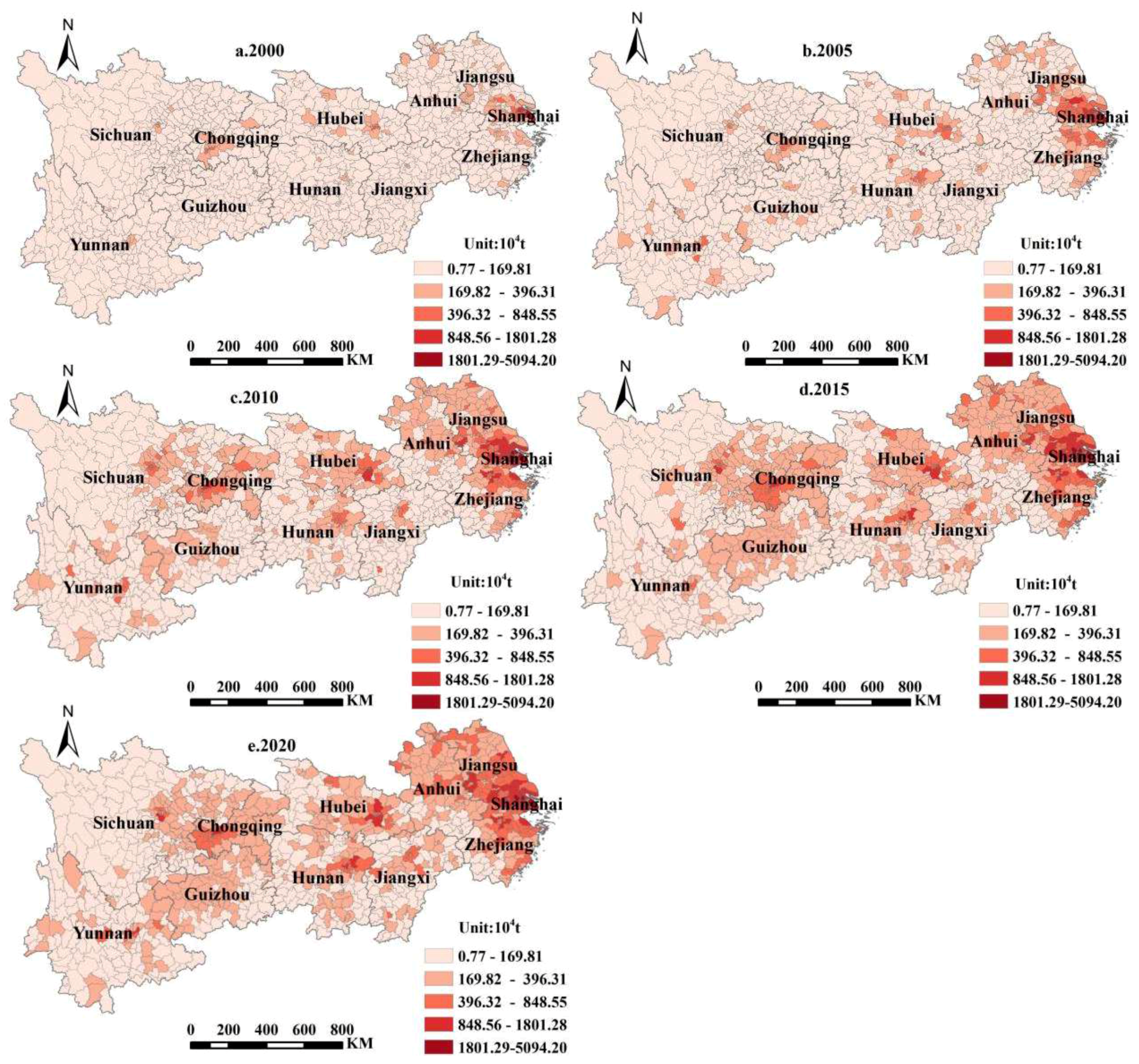
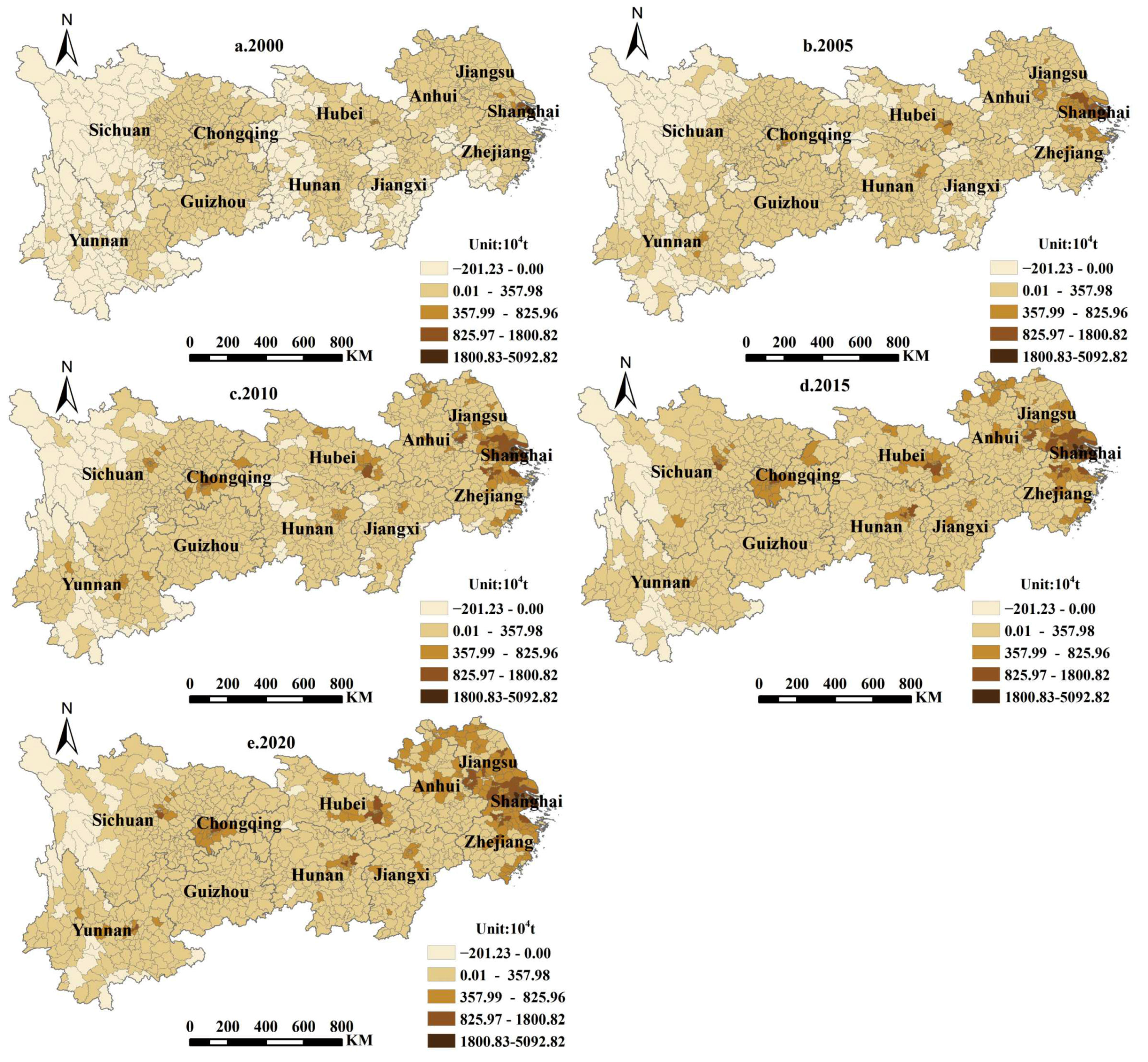
3.1.2. Spatial Evolution Characteristics

The LUCEs in counties within the YREB exhibit a pronounced spatial imbalance (Figure 3), portraying an overarching trend of higher values in the east and lower values in the west. Throughout the entire study period (2000–2020), LUCEs showed a gradual overall increase, yet the absolute disparities among regions were incessantly widening. This phenomenon may be attributed to the rapid development of China’s industrial economy and the continuous escalation of energy consumption, leading to an increasingly conspicuous economic imbalance among regions. Specifically, lower reaches exhibit relatively higher LUCEs in counties, particularly in provinces such as Jiangsu, Zhejiang, and Shanghai. Over time, the high-value regions of LUCEs in counties in the middle and upper reaches further expand. Upon comparison, counties with generally lower LUCEs are predominantly located in the upstream provinces of Sichuan and Yunnan.

The spatial pattern of carbon sinks in land use across YREB counties contrasts with that of the LUCEs (Figure 4), exhibiting higher characteristics in the western regions and lower attributes in the eastern regions. The counties with high carbon sink value are mainly concentrated in Sichuan, Yunnan, and Guizhou provinces in the upper reaches of the Yangtze River and in northern Hubei province in the middle reaches of the Yangtze River, which play an important role in maintaining the ecological security of the YREB [47]. The low carbon sinks are mainly distributed in the downstream Jiangsu province, Shanghai, and Anhui province. On the whole, the spatial change in land use carbon sink in the whole YREB remained stable from 2000 to 2020, indicating that the overall fluctuation of carbon sink had little impact on the overall LUCB.

The spatial characteristics of the LUCB in the YREB are basically consistent with those of carbon emissions (Figure 5), which also indicates that LUCEs in the YREB are the main reason affecting the total LUCB. During 2000–2020, the number of high-value LUCB areas increased, gradually expanding from the lower reaches of the Yangtze River to the middle and upper reaches of the Yangtze River. Specifically, these high-value areas are mainly distributed in the Zhejiang and Jiangsu provinces, including Shanghai, Suzhou, Wuxi, Nantong, Changzhou, Nanjing, Hangzhou, Ningbo, Jinhua, Wuhan, Changsha, Chongqing, Chengdu, Kunming, and so on. These county-level administrative units with high carbon budgets are the key areas for carbon emission control in the YREB.

From the center-of-gravity perspective (Figure 6), the LUCB in counties within the YREB at various characteristic time points is situated between 114°24′21″ E–114°51′39″ E and 30°14′2″ N–30°34′12″ N, predominantly within Hubei province. Examining the trajectory and direction of center-of-gravity migration, the center-of-gravity distribution of the LUCB in the YREB shows an overall southwestward movement. On a phased basis, from 2000 to 2005, the center of gravity moved southward from Huangzhou to Daye; from 2005 to 2015, it continued westward through Liangzi Lake in Wuhan, ultimately reaching Jiangxia; and from 2015 to 2020, it retraced its path from Jiangxia back to Liangzi Lake. This indicates that throughout the entire study period, the LUCB in counties within the middle and upper reaches of the Yangtze River exhibited a growth rate consistently higher than the overall average of the YREB. However, it is noteworthy that the COVID-19 pandemic in 2020 significantly impacted Hubei province, leading to a noticeable decline in the LUCB levels of its counties, thereby causing the phenomenon of center-of-gravity migration reversal.

From 2000 to 2020, the SDE of LUCB in counties within the YREB exhibited a spatial distribution pattern resembling a near “east–west” orientation (Figure 7). In terms of SDE area, the area continuously expanded over the study period, indicating a trend of spatial dispersion in the LUCB of the YREB. In terms of differentiation direction, from 2000 to 2020, the orientation angle of the SDE representing the spatial distribution of the LUCB fluctuated but generally showed a decreasing trend (from 72.79° to 70.89°), with a small change in magnitude. This suggests that the dispersal direction of the LUCB in the YREB remained relatively stable. Regarding the semiaxis lengths, the length of the major semiaxis increased from 858.99 km in 2000 to 876.46 km in 2020, while the length of the minor semiaxis increased from 262.90 km to 289.12 km. This indicates a centripetal aggregation trend in the northeast–southwest direction and a spatial dispersal trend in the northwest–southeast direction for the LUCB in county-level units within the YREB.

Unlike the general spatial differentiation observed in the LUCB across the YREB (Figure 7), the directional attributes of the LUCB in the upper, middle, and lower reaches of the YREB display more distinct tendencies concerning center-of-gravity displacement and shape differentiation. In the lower reaches, the center-of-gravity position remains relatively stable, primarily concentrated around Yixing. The center of gravity in the middle reaches continues its southward migration, shifting from Chibi in Hubei province to Yueyang in Hunan province. Meanwhile, the center of gravity in the upper reaches is mainly concentrated in the southeast of Sichuan province. The SDE in the downstream region primarily exhibits a “northwest–southeast” pattern, contrasting with the orientation of the overall SDE for the YREB. The middle reaches’ SDE shows minimal differences in the lengths of the major and minor axes, indicating a relatively dispersed spatial distribution of the LUCB, likely associated with the small developmental disparities among the three provinces in the middle reaches. In the lower reaches, the distribution direction of the SDE is more similar to that of the overall SDE for the YREB, with a significant increase in its area. In comparison with the entire YREB, the LUCB in counties within the upper reaches exhibits a more distinct trend of dispersion.

3.1.3. Spatial Correlation Analysis

During the research period from 2000 to 2020, Moran’s I indices for the LUCB in counties within the YREB consistently yielded positive values. The mean value of Moran’s I is 0.64, and the p-value passed the test at the 1% significance level. This signifies a significant positive spatial correlation in the LUCB across the YREB, indicating that counties with higher and lower LUCB are spatially adjacent. When observing the temporal trend, the global Moran’s I for LUCB demonstrates an overall fluctuating decline, suggesting a gradual increase in spatial disparities among counties in the YREB.

The spatial distribution characteristics of LUCB in the YREB (Figure 8) reveal a tendency towards clustering in high–high and low–low regions, accompanied by sporadic occurrences in high–low and low–high regions. Broadly, from the year 2000 to 2020, high–high clustering areas were predominantly found in the lower reaches of the Yangtze River, encompassing Zhejiang province, Jiangsu province, and Shanghai. The quantity of such regions shows a consistent upward trajectory, with sporadic instances in the middle reaches around Wuhan and Changsha, as well as downstream in Chongqing and Chengdu. Low–low clustering areas are primarily situated in Sichuan province, Yunnan province, and Jiangxi province, with a secondary concentration in the middle reaches of Hubei and Hunan. Additionally, sporadic occurrences are noted in Zhejiang province downstream. Low–high clustering areas are mainly distributed around high–high clustering regions, with their numbers increasing from 1 in 2000 to 7 in 2020. These areas exhibit lower carbon balance levels but are influenced by positive spillover effects from high-carbon regions. High–low clustering areas are sporadically dispersed in Hunan, Hubei, and Jiangxi in the middle reaches, as well as in Sichuan and Yunnan in the upstream region. The quantity of such areas has increased from 4 in 2000 to 14 in 2020, indicating a reduction in spatial correlation in land use carbon balances at the county level during this period, consistent with Moran’s global I results.

3.2. Coordinated Zoning of the LUCB in the YREB

3.2.1. Spatial Distribution of ECC

The ECC within the YREB exhibits a prevailing pattern with elevated values in the eastern regions and diminished values in the western regions (Figure 9). Counties with ECC < 1 are predominantly concentrated in the upper reaches, specifically in the Sichuan, Yunnan, and Guizhou provinces. These areas exhibit relatively lower levels of economic development, technological sophistication, and energy utilization efficiency, thereby resulting in an ECC smaller than the contribution rates of carbon emissions. In contrast, counties in the middle and upper reaches demonstrate relatively advanced economic development, with technological advancements enhancing energy utilization efficiency. Consequently, the economic contribution in these areas surpasses the contribution of carbon emissions. Based on this, counties with ECC > 1 are primarily distributed in these regions.

During the course of this investigation, the number of county-level units with ECC > 1 declined from 452 in the years 2000–2015 to 362, subsequently rising to 367 in the year 2020. This trend can be attributed to the period from 2000 to 2010, during which China underwent rapid economic growth and urbanization. However, economic development during this period was relatively extensive, characterized by excessive reliance on resource-intensive and highly polluting industries. Particularly, in the YREB, economic growth was concentrated in high-carbon-emission industries such as energy, steel, and coal, leading to substantial carbon emissions. At the same time, escalating urbanization rates have driven the swift enlargement of construction land, intensifying the overexploitation of land resources and negatively influencing carbon emissions. Since 2012, the Chinese government has emphasized sustainable development and ecological civilization construction, progressively undertaking economic restructuring and reinforcing environmental protection measures to alter this carbon-intensive development pattern. However, adjustments to economic and energy structures are gradual processes, and carbon emissions may continue to grow for a certain period. As these adjustments deepen, the rate of carbon emission growth is expected to gradually decrease.

3.2.2. Spatial Distribution of ESC

The ESC observed in YREB counties follows a general trend, with higher values in the western regions and lower values in the eastern regions, showcasing a pattern fundamentally opposite to that of the ECC (Figure 10). Specifically, counties with ESC < 1 are predominantly concentrated in the upper reaches of the Yangtze River, including Sichuan, Yunnan, and Guizhou, as well as the central provinces of Hubei, Hunan, and Jiangxi. These areas boast a commendable ecological foundation, featuring expansive woodland and grassland areas, predominantly characterized by mountainous and hilly terrain, serving as crucial ecological barriers in the YREB. They safeguard the ecological security of not only the region but the entirety of China as well. However, due to their relatively underdeveloped economies, sparse populations, and smaller scales of construction land, these areas exhibit higher ESC.

3.2.3. Coupling Coordination Analysis

Between 2000 and 2020, the coordination between ECC and ESC across counties in the YREB ranged from 0.1710 to 0.1911. In contrast to previous studies at the prefecture level along the Yangtze River, where the coupling coordination ranged from 0.3422 to 0.5691 [14,37,48], the coupling coordination at the county level was inferior, indicating a more pronounced spatial heterogeneity among administrative units at the county level [49]. In comparison with the prefecture level, the counties in the YREB exhibit significant disparities in economic development, industrial structure, and land use patterns, contributing to their lower coupling coordination characteristics.

Upon closer examination, the mean values of coupling coordination for ECC and ESC across counties in the YREB were 0.1827, 0.1721, 0.1911, 0.1844, and 0.1710, respectively, demonstrating a trend of initial decline followed by an ascent and subsequent decline. The peak coupling coordination was observed in 2010, attributable to the simultaneous rapid economic development and rationalization/improvement of economic structures within the YREB. Simultaneously, there was a heightened emphasis on ecological considerations, leading to a substantial increase in the coupling coordination between ECC and ESC. Post-2010, both indicators experienced a reduction in coupling coordination. This phenomenon can be attributed to the fact that, on average across counties in the YREB, as socioeconomic development reaches a certain stage, the contribution rates of carbon emissions and carbon absorption tend to stabilize under equivalent conditions. Conversely, the ESC is constrained by the quality of the regional ecological environment, the formulation and implementation of ecological protection policies, and other factors. Therefore, after reaching a certain stage of development, the ESC of carbon in the YREB weakened due to the influence of these factors. In comparison, the impact on ECC coefficients was less pronounced. This suggests that, except for a few counties that indiscriminately pursue rapid socioeconomic development, resulting in environmental degradation and the weakening of regional ESC, even with the subsequent implementation of ecological protection policies, the process is protracted. As a result, this leads to a reduction in coupling coordination between the two indicators.

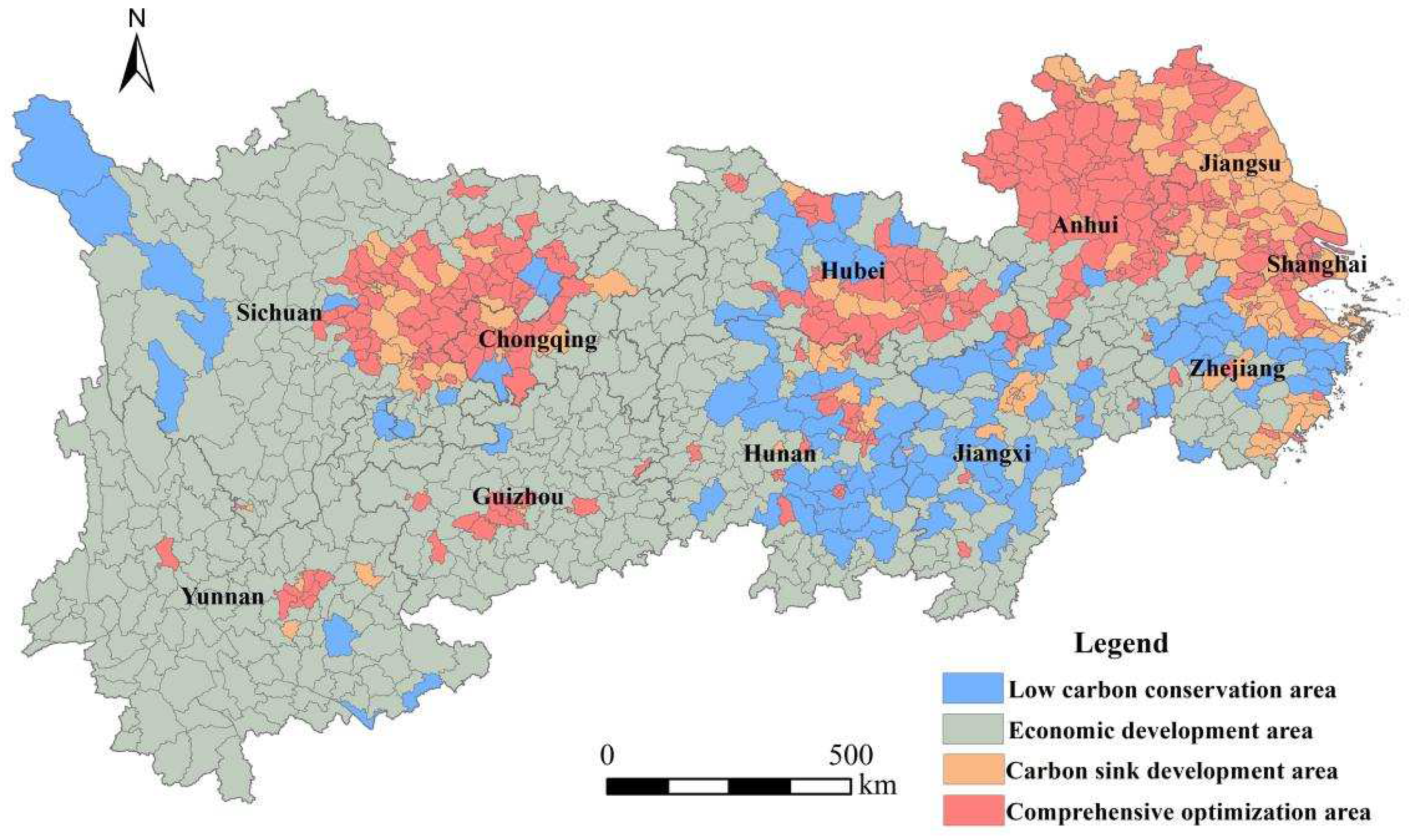
3.2.4. Carbon Emission and Economic Development Zoning

According to the average characteristics of the ECC and ESC in the 5th phase, and referring to previous studies [14,37,50], this paper divides 1069 county units in the YREB into four types of regions: low-carbon conservation area, economic development area, carbon sink development area, and comprehensive optimization area (Figure 11).

When ESC > 1 and ECC > 1, it designates a low-carbon conservation area, predominantly found in Zhejiang province, as well as the central regions of Hunan, Hubei, and Jiangxi provinces. In these locales, carbon productivity and energy utilization exhibit notable efficiency, while the ecological resources supporting carbon sinks are abundantly endowed. The robust capacity for carbon absorption and carrying is evident, striking a relative balance between socioeconomic development and the preservation of ecological resources. Counties falling into the category of low carbon retention areas either possess a strong economic foundation or are endowed with rich tourism resources. It is imperative to sustain the harmonious development of both the economy and the environment. This involves intensifying efforts to protect ecological resources and, concurrently, fostering new energy, high-tech, and ecological industries. The vigorous development of the tertiary sector should be emphasized, facilitating the convergence of leading industries toward low-carbon sectors. Additionally, strategies to enhance the utilization efficiency of land for production and living purposes should be devised, aiming to curtail changes in various land uses.

When ESC > 1 and ECC < 1, it falls within the ambit of an economic development zone. This region’s county units are primarily situated in the downstream areas of the Yangtze River, with notable provinces including Sichuan, Yunnan, and Guizhou. These areas exhibit robust carbon sequestration capabilities, yet their economic contributions to carbon emissions are relatively low, indicative of lower utilization efficiency in areas such as energy. Provinces like Sichuan and Yunnan, functioning as ecological barriers in the YREB, hold heightened ecological significance. Hence, these locales should strive to enhance ecological resources and safeguard ecological functions while advancing the practical development of emerging environmentally friendly industries and eco-tourism. Accelerating the research and introduction of low-carbon technologies, drawing insights from the developmental experiences of provinces in low-carbon retention areas, is recommended. Rational land use planning is crucial, aiming to simultaneously increase carbon productivity and energy utilization efficiency, thereby elevating their ecological barrier functions within the YREB and effectively leveraging their role as carbon sinks.

When ESC < 1 and ECC > 1, these regions fall under the category of carbon sink development area. Counties in this category are predominantly situated in the downstream regions of the Yangtze River, notably in areas like Jiangsu province and Shanghai. There are sporadic instances found in several urban clusters within Chengd–Chongqing and the middle reaches of the Yangtze River. While these areas may exhibit lower carbon absorption capacity, their economic development is relatively robust, accompanied by substantial carbon emissions. Provinces like Shanghai and Jiangsu boast economic prosperity and diverse industries, attracting a significant influx of people from other regions for work and settlement, resulting in high population density and rapid expansion of production and living land use. These regions should vigorously enhance the utilization efficiency of various land types, mitigate the pace of expansion in construction land, and leverage their superior industrial foundation to drive the transformation and upgrading of the industrial structure toward low carbon. Simultaneously, leveraging their advanced technological foundation, they can promote technological innovation in manufacturing. Continuing the emphasis on clean energy sources such as natural gas, reducing the proportion of high-carbon and traditional energy usage, and rigorously protecting ecological resources while planning to increase ecological land use will contribute to enhancing their carbon sink capabilities.

When ESC < 1 and ECC < 1, the region falls into the category of comprehensive optimization area. Counties of this category are predominantly found in the southeastern region of Hubei province, situated in the middle reaches of the Yangtze River, and in the southeastern part of Sichuan province, located in the upper reaches. Overall, these areas exhibit relatively low carbon economic contributions and limited carbon absorption capacity. Despite some counties being home to provincial capital cities such as Wuhan in Hubei province and Chengdu in Sichuan province, these areas, while experiencing generally high economic development, also generate significant carbon emissions. Therefore, overall, these regions should focus on controlling carbon emissions and promoting green development. By restricting the development of industries with high carbon emissions and low energy utilization rates and simultaneously investing in scientific and technological advancements while incorporating exemplary low-carbon practices, the aim is to transform production processes, enhance energy efficiency, optimize industrial layouts, leverage policy or geographical advantages to foster industrial agglomeration, and form circular industrial chains, thereby reducing carbon emissions. Strengthening the management and protection of ecological resources, expanding ecological land use such as forests and grasslands, restoring and enhancing carbon sink ecosystems, increasing carbon absorption capacity, and promoting low-carbon sustainable development are crucial aspects of the comprehensive optimization strategy.

4. Conclusions

This study focused on 1069 county-level units within the YREB and conducted an analysis of the spatiotemporal characteristics of the LUCB for these units. Additionally, a regional study was conducted by examining the ECC of carbon emissions, ESC, and their coupling relationship. The following conclusions were drawn.

Between 2000 and 2020, the total LUCEs in the YREB exhibited significant growth. Constructed land stands as the primary source of carbon emissions, while woodlands serve as the principal contributors to carbon sequestration. The spatial distribution of LUCEs in the counties along the YREB presents an “east high, west low” pattern, in stark contrast to the spatial configuration of carbon sinks. The spatial center of gravity for the LUCB across county units in the YREB moved predominantly toward the southwest. This spatial arrangement exhibits positive spatial autocorrelation, featuring significant spatial clustering, primarily in the form of high–high and low–low aggregation. The YREB’s county units showcase a pattern where the ECC displays an “east high, west low” characteristic, while the ESC exhibits a “west high, east low” feature, indicating a relatively low degree of coordination between the two. Based on the ECC and ESC coefficients, this paper categorizes the county units into low-carbon conservation areas, areas for economic development, carbon sink development areas, and comprehensive optimization areas.

Some limitations persist: In the estimation of carbon sinks, a uniform coefficient from previous studies is applied to various land uses, yet substantial regional disparities exist across the entire YREB. Consequently, the carbon emission coefficients for land use may not perfectly align with the actual regional conditions, introducing potential errors in the calculated carbon emissions. Additionally, due to data limitations, the carbon emissions or absorption from cropland, particularly the emissions from plants within cultivated land, were not considered. Furthermore, in the recommendations for zoning optimization, a comprehensive multi-indicator system was not established. Therefore, future research endeavors should delve further into these aspects for a more nuanced understanding.

References

1. van Soest, H.L.; den Elzen MG, J.; van Vuuren, D.P. Net-zero emission targets for major emitting countries consistent with the Paris Agreement. Nat. Commun. 2021, 12, 2140. [Google Scholar] [CrossRef] [PubMed]
2. Wang, Y.; Guo, C.; Chen, X.; Jia, L.Q.; Guo, X.; Chen, R.S.; Zhang, M.S.; Chen, Z.; Wang, H.D. Carbon peak and carbon neutrality in China: Goals, implementation path and prospects. China Geol. 2021, 4, 720–746. [Google Scholar] [CrossRef]
3. Zhao, X.; Ma, X.; Chen, B.; Shang, Y.; Song, M. Challenges toward carbon neutrality in China: Strategies and counter measures. Resour. Conserv. Recycl. 2022, 176, 105959. [Google Scholar] [CrossRef]
4. Hong, C.; Burney, J.A.; Pongratz, J.; Nabel, J.E.M.S.; Mueller, N.D.; Jackson, R.B.; Davis, S.J. Global and regional drivers of land-use emissions in 1961–2017. Nature 2021, 589, 554–561. [Google Scholar] [CrossRef] [PubMed]
5. Ruehr, S.; Keenan, T.F.; Williams, C.; Zhou, Y.; Lu, X.; Bastos, A.; Canadell, J.G.; Prentice, I.C.; Sitch, S. Evidence and attribution of the enhanced land carbon sink. Nat. Rev. Earth Environ. 2023, 4, 518–534. [Google Scholar] [CrossRef]
6. Jiang, Y.; Sun, Y.; Liu, Y.; Li, X. Exploring the correlation between waterbodies, green space morphology, and carbon dioxide concentration distributions in an urban waterfront green space: A simulation study based on the carbon cycle. Sustain. Cities Soc. 2023, 98, 104831. [Google Scholar] [CrossRef]
7. Piao, S.; He, Y.; Wang, X.; Chen, F. Estimation of China’s terrestrial ecosystem carbon sink: Methods, progress and prospects. Sci. China Earth Sci. 2022, 65, 641–651. [Google Scholar] [CrossRef]
8. Bultan, S.; Nabel, J.E.M.S.; Hartung, K.; Ganzenmüller, R.; Xu, L.; Saatchi, S.; Pongratz, J. Tracking 21st-century anthropogenic and natural carbon fluxes through model-data integration. Nat. Commun. 2022, 13, 5516. [Google Scholar] [CrossRef]
9. Gidden, M.J.; Gasser, T.; Grassi, G.; Forsell, N.; Janssens, I.; Lamb, W.F.; Minx, J.; Nicholls, Z.; Steinhauser, J.; Riahi, K. Aligning climate scenarios to emissions inventories shifts global benchmarks. Nature 2023, 624, 102–108. [Google Scholar] [CrossRef]
10. Yang, H.; Chen, W. Spatio-temporal pattern of urban vegetation carbon sink and driving mechanisms of human activities in Huaibei, China. Environ. Sci. Pollut. Res. 2022, 29, 31957–31971. [Google Scholar] [CrossRef]
11. Mishra, U.; Torn, M.S.; Masanet, E.; Ogle, S.M. Improving regional soil carbon inventories: Combining the IPCC carbon inventory method with regression kriging. Geoderma 2012, 189–190, 288–295. [Google Scholar] [CrossRef]
12. Samariks, V.; Lazdiņš, A.; Bārdule, A.; Kalēja, S.; Butlers, A.; Spalva, G.; Jansons, Ā. Impact of Former Peat Extraction Field Afforestation on Soil Greenhouse Gas Emissions in Hemiboreal Region. Forests 2023, 14, 184. [Google Scholar] [CrossRef]
13. Köne, A.Ç.; Büke, T. Factor analysis of projected carbon dioxide emissions according to the IPCC-based sustainable emission scenario in Turkey. Renew. Energy 2019, 133, 914–918. [Google Scholar] [CrossRef]
14. Wu, H.; Deng, K.; Dong, Z.; Meng, X.; Zhang, L. Comprehensive assessment of land use carbon emissions of a coal resource-based city, China. J. Clean. Prod. 2022, 379, 134706. [Google Scholar] [CrossRef]
15. Spawn, S.A.; Lark, T.J.; Gibbs, H.K. Carbon emissions from cropland expansion in the United States. Environ. Res. Lett. 2019, 14, 45009. [Google Scholar] [CrossRef]
16. Castaño-Sánchez, J.P.; Izaurralde, R.C.; Prince, S.D. Land-use conversions from managed grasslands to croplands in Uruguay increase medium-term net carbon emissions to the atmosphere. J. Land Use Sci. 2021, 16, 240–259. [Google Scholar] [CrossRef]
17. Wang, H.H.; He, Y.Y.; Shi, W.Y.; Zeng, W.; He, Y. Spatiotemporal spillover effect and efficiency of carbon emissions from land use in China. Environ. Dev. Sustain. 2023, 1–39. [Google Scholar] [CrossRef]
18. Wu, S.; Hu, S.G.; Frazier, A.E. Spatiotemporal variation and driving factors of carbon emissions in three industrial land spaces in China from 1997 to 2016. Technol. Forecast. Soc. Chang. 2021, 169, 120837. [Google Scholar] [CrossRef]
19. Houghton, R.A.; House, J.I.; Pongratz, J.; Van Der Werf, G.R.J.; Defries, R.S.; Hansen, M.; Le, Q.C. Carbon emissions from land use and land-cover change. Biogeosciences 2012, 9, 5125–5142. [Google Scholar] [CrossRef]
20. Yue, T.; Long, R.Y.; Chen, H.; Zhao, X. The optimal CO2 emissions reduction path in Jiangsu province: An expanded IPAT approach. Appl. Energy 2013, 112, 1510–1517. [Google Scholar] [CrossRef]
21. Feng, Y.; Chen, S.; Tong, X.; Lei, Z.K.; Gao, C.; Wang, J.F. Modeling changes in China’s 2000–2030 carbon stock caused by land use change. J. Clean. Prod. 2020, 252, 119659. [Google Scholar] [CrossRef]
22. Trainor, A.M.; Mcdonald, R.I.; Fargione, J. Energy Sprawl Is the Largest Driver of Land Use Change in United States. PLoS ONE 2016, 11, e162269. [Google Scholar] [CrossRef]
23. Diao, J.; Liu, J.; Zhu, Z.; Li, M.; Sleeter, B.M. Substantially Greater Carbon Emissions Estimated Based on Annual Land-Use Transition Data. Remote Sens. 2020, 12, 1126. [Google Scholar] [CrossRef]
24. Li, H.; Zhao, Y.H.; Wang, S.; Liu, Y. Spatial-temporal characteristics and drivers of the regional residential CO2 emissions in China during 2000–2017. J. Clean. Prod. 2020, 276, 124116. [Google Scholar] [CrossRef]
25. Yue, C.; Ciais, P.; Houghton, R.A.; Nassikas, A.A. Contribution of land use to the interannual variability of the land carbon cycle. Nat. Commun. 2020, 11, 3170. [Google Scholar] [CrossRef] [PubMed]
26. Wang, P.; Wu, W.S.; Zhu, B.Z.; Wei, Y. Examining the impact factors of energy-related CO2 emissions using the STIRPAT model in Guangdong Province, China. Appl. Energy 2013, 106, 65–71. [Google Scholar] [CrossRef]
27. Lv, Q.; Liu, H.; Wang, J.; Liu, H.; Shang, Y. Multiscale analysis on spatiotemporal dynamics of energy consumption CO2 emissions in China: Utilizing the integrated DMSP-OLS and NPP-VIIRS nighttime light datasets. Sci. Total Environ. 2020, 703, 134394. [Google Scholar] [CrossRef]
28. Bi, Y.; Zheng, L.; Wang, Y.; Li, J.; Yang, H.; Zhang, B. Coupling relationship between urbanization and water-related ecosystem services in China’s Yangtze River Economic Belt and its socio-ecological driving forces: A county-level perspective. Ecol. Indic. 2023, 146, 109871. [Google Scholar] [CrossRef]
29. Lin, Y.; Peng, C.; Shu, J.; Zhai, W.; Cheng, J. Spatiotemporal characteristics and influencing factors of urban resilience efficiency in the Yangtze River Economic Belt, China. Environ. Sci. Pollut. Res. 2022, 29, 39807–39826. [Google Scholar] [CrossRef]
30. Yang, X.; Feng, Z.; Chen, Y. Evaluation and obstacle analysis of high-quality development in Yellow River Basin and Yangtze River Economic Belt, China. Humanit. Soc. Sci. Commun. 2023, 10, 757. [Google Scholar] [CrossRef]
31. Zhou, Y.; Zhong, Z.; Cheng, G. Cultivated land loss and construction land expansion in China: Evidence from national land surveys in 1996, 2009, and 2019. Land Use Policy 2023, 125, 106496. [Google Scholar] [CrossRef]
32. Li, L.; Li, J.F.; Peng, L.; Wang, X.; Sun, S. Spatiotemporal evolution and influencing factors of land-use emissions in the Guangdong-Hong Kong-Macao Greater Bay Area using integrated nighttime light datasets. Sci. Total Environ. 2023, 893, 164723. [Google Scholar] [CrossRef] [PubMed]
33. Fang, J.Y.; Guo, Z.D.; Piao, S.L.; Chen, A.P. Terrestrial vegetation carbon sinks in China, 1981–2000. Sci. China Ser. D Earth Sci. 2007, 50, 1341–1350. [Google Scholar] [CrossRef]
34. Sun, H.; Liang, H.M.; Chang, X.L.; Cui, Q.; Tao, Y. Land Use Patterns on Carbon Emission and Spatial Association in China. Econ. Geogr. 2015, 35, 154–162. [Google Scholar]
35. Qi, S.; Fu, K. Comparative Analysis of the Accounting Method of Provincial Carbon Emission During the Low Carbon Transition. Wuhan Univ. J. (Philos. Soc. Sci.) 2013, 66, 85–92. (In Chinese) [Google Scholar]
36. Meng, L.; Graus, W.; Worrell, E.; Huang, B. Estimating CO2 (carbon dioxide) emissions at urban scales by DMSP/OLS (Defense Meteorological Satellite Program’s Operational Linescan System) nighttime light imagery: Methodological challenges and a case study for China. Energy 2014, 71, 468–478. [Google Scholar] [CrossRef]
37. Xiong, S.; Yang, F.; Li, J.; Xu, Z.; Ou, J. Temporal-spatial variation and regulatory mechanism of carbon budgets in territorial space through the lens of carbon balance: A case of the middle reaches of the Yangtze River urban agglomerations, China. Ecol. Indic. 2023, 154, 110885. [Google Scholar] [CrossRef]
38. Mathur, M. Spatial autocorrelation analysis in plant population: An overview. J. Appl. Nat. Sci. 2015, 7, 501–513. [Google Scholar] [CrossRef]
39. Ord, J.K.; Getis, A. Testing for local spatial autocorrelation in the presence of global autocorrelation. J. Reg. Sci. 2001, 41, 411–432. [Google Scholar] [CrossRef]
40. Huang, H.; Zhou, J. Study on the spatial and temporal differentiation pattern of carbon emission and carbon compensation in China’s provincial areas. Sustainability 2022, 14, 7627. [Google Scholar] [CrossRef]
41. Cui, D.; Chen, X.; Xue, Y.; Xue, Y.; Li, R.; Zeng, W. An integrated approach to investigate the relationship of coupling coordination between social economy and water environment on urban scale-A case study of Kunming. J. Environ. Manag. 2019, 234, 189–199. [Google Scholar] [CrossRef] [PubMed]
42. Wang, H.; Lu, X.; Deng, Y.; Sun, Y.G.; Nielsen, C.P.; Liu, Y.F.; Zhu, G.; Bu, M.L.; Bi, J.; McElroy, M.B. China’s CO2 peak before 2030 is implied by the characteristics and growth of cities. Nat. Sustain. 2019, 2, 748–754. [Google Scholar] [CrossRef]
43. Cui, F.; Wang, Y.; Liu, G. Exploring the spatial–temporal evolution and driving mechanisms for coupling coordination between the green transformation of urban construction land and industrial transformation and upgrading: A case study of the urban agglomeration in the middle reaches of the Yangtze River. Environ. Sci. Pollut. Res. 2023, 30, 119385–119405. [Google Scholar]
44. Xie, Z. China’s historical evolution of environmental protection along with the forty years’ reform and opening-up. Environ. Sci. Ecotechnol. 2020, 1, 100001. [Google Scholar] [CrossRef]
45. Rao, C.; He, Y.; Wang, X. Comprehensive Evaluation of Non-waste Cities Based on Two-Tuple Mixed Correlation Degree. Int. J. Fuzzy Syst. 2021, 23, 369–391. [Google Scholar] [CrossRef]
46. Zhao, J.; Zhao, Y. Synergy/trade-offs and differential optimization of production, living, and ecological functions in the Yangtze River economic Belt, China. Ecol. Indic. 2023, 147, 109925. [Google Scholar] [CrossRef]
47. Gao, Y.; Wang, Z.; Xu, F. Geospatial characteristics and the application of land use functions in the Yangtze River Economic Belt, China: Perspectives on provinces and urban agglomerations. Ecol. Indic. 2023, 155, 110969. [Google Scholar] [CrossRef]
48. Yuan, S.F.; Tang, Y.Y. Spatial Differentiation of Land Use Carbon Emission in the Yangtze River Economic Belt Based on Low Carbon Perspective. Econ. Geogr. 2019, 39, 190–198. (In Chinese) [Google Scholar]
49. Shi, K.; Chen, Y.; Yu, B.; Xu, T.; Chen, Z.; Liu, R.; Li, L.; Wu, J. Modeling spatiotemporal CO2 (carbon dioxide) emission dynamics in China from DMSP-OLS nighttime stable light data using panel data analysis. Appl. Energy 2016, 168, 523–533. [Google Scholar] [CrossRef]
50. Li, Y.Y.; Wei, W.; Zhou, J.J.; Hao, R.J.J.; Chen, D.B. Changes in Land Use Carbon Emissions and Coordinated Zoning in China. Environ. Sci. 2023, 44, 1267–1276. (In Chinese) [Google Scholar]
Figure 1. Location map of the YREB: (a) map of China’s regional location; (b) main functional zoning map of the YREB; (c) digital elevation model (DEM) of the YREB.
Land 13 00215 g001
Figure 2. Changes in LUCB in the YREB from 2000 to 2020: (a) changes in carbon emissions, carbon sinks, and carbon budget in the YREB and (b) proportion of carbon emissions, carbon sinks, and carbon budget in different zones of the YREB.
Land 13 00215 g002
Figure 3. Spatial distribution of LUCEs in the YREB: (a) spatial distribution of LUCEs in the year 2000; (b) spatial distribution of LUCEs in the year 2005; (c) spatial distribution of LUCEs in the year 2010; (d) spatial distribution of LUCEs in the year 2015; (e) spatial distribution of LUCEs in the year 2020.
Land 13 00215 g003
Figure 4. Spatial distribution of land use carbon sink in the YREB: (a) spatial distribution of land use carbon sink in the year 2000; (b) spatial distribution of land use carbon sink in the year 2005; (c) spatial distribution of land use carbon sink in the year 2010; (d) spatial distribution of land use carbon sink in the year 2015; (e) spatial distribution of land use carbon sink in the year 2020.
Land 13 00215 g004
Figure 5. Spatial distribution of LUCB in the YREB from 2000 to 2020: (a) spatial distribution of LUCB in the year 2000; (b) spatial distribution of LUCB in the year 2005; (c) spatial distribution of LUCB in the year 2010; (d) spatial distribution of LUCB in the year 2015; (e) spatial distribution of LUCB in the year 2020.
Land 13 00215 g005
Figure 6. Transfer path of LUCB in the YREB.
Land 13 00215 g006
Figure 7. Transfer path of LUCB in the YREB (upper reaches, middle reaches, and lower reaches).
Land 13 00215 g007
Figure 8. LISA aggregation of LUCB in the YREB: (a) LISA aggregation of LUCB in the year 2000; (b) LISA aggregation of LUCB in the year 2005; (c) LISA aggregation of LUCB in the year 2010; (d) LISA aggregation of LUCB in the year 2015; (e) LISA aggregation of LUCB in the year 2020.
Land 13 00215 g008
Figure 9. Spatial distribution of ECC in the YREB: (a) spatial distribution of ECC in the year 2000; (b) spatial distribution of ECC in the year 2005; (c) spatial distribution of ECC in the year 2010; (d) spatial distribution of ECC in the year 2015; (e) spatial distribution of ECC in the year 2020.
Land 13 00215 g009
Figure 10. Spatial distribution of ESC in the YREB: (a) spatial distribution of ESC in the year 2000; (b) spatial distribution of ESC in the year 2005; (c) spatial distribution of ESC in the year 2010; (d) spatial distribution of ESC in the year 2015; (e) spatial distribution of ESC in the year 2020.
Land 13 00215 g010
Figure 11. Zoning optimization of LUCB in counties of the YREB.
Land 13 00215 g011
Disclaimer/Publisher’s Note: The statements, opinions and data contained in all publications are solely those of the individual author(s) and contributor(s) and not of MDPI and/or the editor(s). MDPI and/or the editor(s) disclaim responsibility for any injury to people or property resulting from any ideas, methods, instructions or products referred to in the content.