Abstract
Intensive production landscapes provide low levels of many ecosystem services and support limited biodiversity, so they require restoration to enhance their multifunctionality. International guidelines suggest that restoration should aim to establish natural woody vegetation cover across 30% of landscapes. Such restoration may be implemented in varied spatial configurations and complemented by additional land use changes from intensive to extensive semi-natural pastoral grasslands. To restore multifunctional landscapes, we need to understand the impacts of restoration spatial configuration and complementary grassland extensification, both in isolation and in combination. We used a virtual landscape simulation to systematically analyse the impacts of alternative restoration strategies on the provision of nine indicators of ecosystem services and biodiversity, and the overall multifunctionality of the landscapes. All restored landscapes achieved improvements in the performance of individual ecosystem services and multifunctionality compared to the baseline. The benefits of a given restored natural vegetation effort were increased by adding extensive grassland and modifying the spatial configuration of restoration. Randomly distributed patterns of restoration provided higher multifunctionality than restoration adjacent to existing natural areas or as large land blocks. The virtual landscape approach allowed systematic exploration of alternative restoration strategies, providing a mechanistic understanding that will inform restoration tailored to local priorities and conditions.
1. Introduction
Intensive production landscapes have only a small fraction of their original native ecosystems remaining, with natural forests, scrub, and grassland replaced by crops and intensive pastures [1,2,3]. As a result, these landscapes provide little support for biodiversity and suffer reduced provision of critical ecosystem services upon which human well-being relies [4,5,6]. The current unsustainable situation across many intensive production landscapes will worsen with future climate challenges, requiring substantial changes in landscape design to ensure that future landscapes will be “climate-smart” [7,8]. To ensure that production landscapes adapt to the pressures of climate change in the future, we must restore some natural and semi-natural ecosystem cover within them to enhance their ecosystem service multifunctionality [9,10,11].
Restoring natural woody ecosystems is a prevalent target in policy and for land owners because it can improve ecosystem service functionality in production landscapes, benefitting multiple objectives, including global climate regulation, water regulation, microclimate regulation, long-term soil fertility, landscape aesthetics, and biodiversity [12,13,14,15]. Previous research has set targets for the ideal quantity of natural woody ecosystem cover that we need within certain landscapes; for example, it has been recommended that landscapes include at least 40% forest cover to support biodiversity [16] and at least 20% natural habitat cover in agricultural landscapes to ensure satisfactory outcomes for biodiversity, ecosystem services, and food security [6,17]. In Australian production landscapes, a target of 30% natural woody cover has been proposed [18]. Targets for natural vegetation cover have been incorporated into formal policies and legislation; for example, the EU Biodiversity Strategy for 2030 has proposed an overall target to protect at least 30% of land cover for biodiversity [19], and India’s National Forest Policy targets national forest cover of at least 33% [20]. Despite some consensus that the percentage of natural woody vegetation cover required to deliver multifunctional production landscapes probably lies between 20% and 40%, there is little agreement about how restored vegetation should be arranged spatially—although one study recommended that 10% of the landscape area should be made up of large forest patches [16]. The spatial configuration of landscape elements is critical in impacting the provision of some ecosystem services [21,22,23,24] and can, therefore, be expected to impact landscape multifunctionality [25,26].
Woody vegetation restoration can be supplemented by the additional establishment of extensive grasslands (typically including a combination of domesticated and native plant species). Extensive grasslands are an intermediary land use that simultaneously provides agricultural production alongside some regulating and cultural services [3,9]. For Australian biodiversity objectives, it has been recommended that 20% of the landscape area should be allocated for low-intensity production, in addition to the woody vegetation targets [18]. However, little research has focused on the complementary benefits of restoring extensive grassland cover alongside woody vegetation.
While there are almost infinite possible spatial configurations for implementing restoration across a landscape, the available options are constrained by biophysical land suitability, as well as technical, economic, social, and institutional factors [27,28]. In this article, we compare three spatial patterns of restoration that have occurred or been proposed in real-world situations: (1) restoration at random locations, (2) restoration contiguous to existing natural areas, and (3) restoration in large blocks. If restoration is implemented without spatial planning or develops opportunistically as land parcels become available, we might expect to see a random or quasi-random pattern of restored ecosystems across a landscape [29,30]. Alternatively, restored areas may be planned to be adjacent or close to existing fragments of remnant natural vegetation to enlarge the size of these vegetation patches. This strategy may provide buffer regions that protect sensitive species populations or reduce human–wildlife conflicts [31] or be desired if the restoration scheme aims to increase the species richness of taxa that exhibit a positive species–area relationship [32] or to conserve species requiring habitat patches of a certain size [33,34]. Finally, landscape restoration could be planned to allocate large contiguous blocks of land for restoration through a “land-sparing” approach [35]. Land-sparing may enhance biodiversity outcomes due to larger habitat patch sizes [32] and support greater ecosystem service provision than alternative “land-sharing” approaches [36,37]. Furthermore, restoration of large blocks may be likely in some human societies—for example, in cases where a single owner of a large contiguous area retires, emigrates, or covenants land for conservation, thus providing an opportunity to restore a large area [38]. Alternatively, separate landowners that are geographically co-located may make similar decisions towards restoration, either through the organic transfer of information and ideas through social networks or formal partnerships arranged by conservation organisations [39,40,41].
Simulation modelling can assess alternative restoration scenarios for a given landscape by comparing the performance of alternative restoration coverage and configuration options [42,43,44]. This place-based approach is an important step in knowledge development, but local specificities and constraints may limit the range of options that are considered and the generalisation of the findings. Case study syntheses are essential for generalisation [45,46,47] but are limited by available situations and observations. To establish a more general understanding, virtual experiments using hypothetical landscapes are increasingly used to explore interactions between landscape characteristics and the provision of multiple ecosystem services [26,48,49,50,51]. Virtual landscape experiments can provide systematic understanding through a quasi-experimental approach that overcomes local specificities and constraints, allows replication, and can allow testing of a broader range of possibilities [26,51]. Virtual landscape experiments have not yet been applied to analyse how the configuration of woody vegetation and extensive grassland restoration interact to impact restoration outcomes at landscape scales [26,48,49,50,51].
Here, we apply a virtual landscape modelling approach to quantify the impacts of the spatial configuration of restoration, as well as complementary extensive grassland restoration in modifying the effects of woody vegetation restoration. We hypothesised that the area of the woody vegetation restored would have the greatest impact on individual indicator outcomes and multifunctionality. We hypothesised that the restoration of extensive grassland would deliver further benefits and that the restoration area effects would be significantly modified by the spatial configuration of the restoration.
2. Materials and Methods
We designed a virtual experiment with three variables describing the restoration strategy (Figure 1). First, we considered two levels of effort for woody vegetation restoration at 10% and 20% of the total landscape area. The 20% woody restoration level achieves the recommendation of providing a total of 30% woody vegetation cover, with the 10% restoration level providing a less ambitious comparison. This lower level of restoration effort may nonetheless achieve some benefits while requiring less agricultural production to be lost. To test the added value of incorporating some complementary restoration of extensive grasslands, we compared two treatments combined with each woody restoration level: no extensive grassland restoration and extensive grassland restoration of an additional third of the natural vegetation area. Finally, to test the influence of spatial configuration of restoration design, we compared three spatial strategies: random spatial locations, targeting restoration contiguous to existing natural woody or extensive grassland vegetation, and restoration in large blocks. These three factors were compared in a factorial design and analysed for their performance across nine ecosystem service and biodiversity indicators, as well as emergent indicators of multifunctionality.
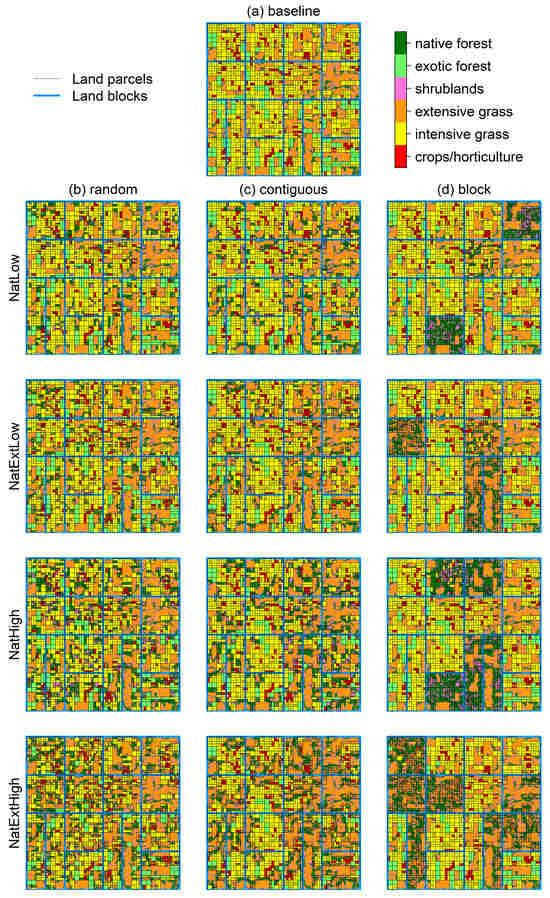
Figure 1.
Example of the creation of (a) one virtual intensive landscape and an associated 12 restoration scenarios (b:d). Twelve restored landscape realisations were generated that factorially combined four restoration land cover percentages with three spatial restoration strategies: (b) random, (c) contiguous, and (d) block configuration. Individual land parcels resulting from the binary space portioning are shown, as well as their higher-level grouping, which formed the basis of the block restoration strategy. NatLow = natural restoration low with no extensive grassland; NatHigh = natural restoration high with no extensive grassland; NatExtLow = natural restoration low with additional extensive grassland target; NatExtHigh = natural restoration high with additional extensive grassland target.
2.1. Virtual Landscape Creation
Virtual landscapes were generated by sequentially creating topographies, river networks, land parcels, and vegetation covers to create realistic but hypothetical maps for common livestock production landscapes [26,52]. The virtual landscapes were created in Python using the NumPy [53], SciPy [54], scikit-image [55], NLMpy [56], GDAL [57], and RichDEM [58] packages. Each stage in the virtual landscape creation process is outlined in the following sub-sections. We created 50 different baseline topographies.
2.1.1. Topography
Each virtual landscape had dimensions of 2000 × 2000 cells with 25 m grain and, therefore, 50 × 50 km extent. The topography of each landscape was generated using a Perlin noise-neutral landscape model [52] parameterised to produce hilly landscape features (periods = 10, octaves = 5, persistence = 0.4) that were rescaled to range from 100 to 800 m. An overall fixed slope with an elevation range of between 0 and 100 m was added to ensure that water would flow consistently out of the landscape. River channels draining areas of at least 3.75 km2 were identified using flow accumulation analysis of the topographic layer [58].
2.1.2. Baseline Landscapes
The starting point of our simulations was intensive livestock production landscapes common throughout temperate regions of Western Europe, Eastern Australia, or New Zealand, with predominant cover of intensive agriculture made mostly of intensive grassland with a small crop component. To produce initial land cover distributions for each topography, binary space partitioning was used to divide the landscape into 2000 rectilinear parcels. These parcels represent human decision-making units such as paddocks or fields. The probability p of partitioning was based on elevation x using the logistic function
to target partitioning and, hence, smaller parcels at lower elevations [52]. The human-dominated land covers of crops/horticulture, intensive grass, and exotic forests were added sequentially to parcels within the landscape [52]. For each land cover, the initial parcel was randomly selected from among the smallest in size across the landscape (parcels with binary space partition length = maximum). The land cover was then expanded by selecting the nearest parcel of a similar size, and this process was repeated until each land cover class had reached its specified maximum proportion of the landscape: crops/horticulture 6%, intensive grass 54%, and forest plantation 10%. The (semi-)natural land covers of extensive grass, natural scrub, and natural forest were assigned to the remainder of the landscape based on a gradient formed by the slope of the topography. Extensive grass was assigned to 20% of the flattest parts of the landscape, natural forest was assigned to 5% of the steepest parts of the landscape, and scrub was assigned to the remaining 5% of the landscape that had intermediate slopes.
2.1.3. Restoration Scenarios
We conducted matched restoration experiments for each of the 50 baseline landscapes by converting human-dominated land covers (crops/horticulture, intensive grass, and forest plantation) into (semi-)natural land covers (extensive grass, natural scrub, and natural forest). We generated 12 restoration realisations for each baseline by a factorial combination of two restoration land cover targets, two extensive grassland targets, and three different spatial restoration strategies (Table 1; Figure 1). We assume that the societal context of the baseline landscapes has garnered sufficient support for restoration of some degree of native woody vegetation cover and is willing to make the necessary trade-off with intensive production. Variation in the restored land area was made up of two treatments representing different levels of restoration effort, with the larger restored area treatment reaching the hypothesised target of a total of 30% of natural woody vegetation cover [18]. Variation in extensive grassland restoration was made up of two treatments representing the exclusion or not of extensive grassland in restoration schemes. The inclusion of extensive grassland in restoration has been proposed as an intermediary land use that provides a mid-point between intensive and natural land cover [3,9]. When extensive grassland was included in restoration schemes, the area of extensive grassland restored was one additional third of the area of natural woody vegetation restored (Table 1). The restoration configuration variable encompasses three treatments that represent the random, contiguous existing natural cover and large block strategies outlined in the Introduction.

Table 1.
Percentages of the landscape restored for each natural land cover and total area restored under four restoration scenarios representing factorial combinations of the natural woody vegetation restored area and extensive grassland inclusion variables.
Random restoration selected human-dominated parcels at random until enough parcels had been selected to meet the area target. Random restoration was designed to provide an aspatial null model where restoration has no spatial planning. Contiguous restoration was designed to mimic expansion of existing natural areas, as recommended for increasing habitat patch size and connectivity [59]. Contiguous restoration randomly selected human-dominated parcels adjacent to existing natural land covers until either enough parcels had been selected or all parcels adjacent to existing natural land covers had been selected. Block restoration was designed to mimic restoration in which entire properties or administrative units were restored, reflecting potential public or private decisions for land conversion. Block restoration was concentrated into large contiguous blocks of around 150 km2 by randomly selecting parcels within higher-level groupings of parcels (binary space partition height = 4) until enough parcels had been selected. Once the parcels for restoration had been selected, natural land covers of the appropriate proportions were assigned by slope as per the initial land cover allocation.
2.2. Landscape Performance Indicators
We modelled nine landscape performance indicators, including six indicators of ecosystem services, two indicators of bird conservation, and one indicator of agricultural profitability. The outcomes of multifunctionality assessments are sensitive to the selection of indicators used [60]. Indicator selection can be challenging for virtual landscapes because, as hypothetical constructs, they lack a societal and economic context with which to inform the prioritisation [26]. We developed nine indicators of landscape performance, a greater number than typically analysed in multifunctionality analyses [60]. We situated our virtual landscapes within Aotearoa, New Zealand, and selected indicators known to be important within the country, using methods that have been previously used in the country (see specific Section 2.2.1, Section 2.2.2, Section 2.2.3, Section 2.2.4, Section 2.2.5, Section 2.2.6, Section 2.2.7 and Section 2.2.8 below). Moreover, our indicators were associated with different types of models that responded in contrasting ways to landscape spatial configuration and were, therefore, expected to be sensitive to alternative landscape restoration strategies [26,61]. We included three indicators based on look-up tables which may be expected to show no effect of spatial landscape configuration (carbon stocks, greenhouse gas emissions, agricultural profitability), two indicators based on models that incorporate topographic relationships (erosion, nutrient retention), two indicators based on models that incorporate spatial dependencies such as supply–demand proximity (pollination) and patch size (recreation), and two indicators where spatial connectivity between landscape patches is explicitly modelled (habitat suitability for two New Zealand indigenous bird species: brown kiwi Apteryx mantelli and kererū Hemiphaga novaeseelandiae). We modelled potential supply capacity for these indicators parameterised with New Zealand data (Supplementary Table S1), using the methods from our previous analysis of virtual landscape ecosystem services [26]. A concise summary of the methods is provided here, with further details found in the references listed.
2.2.1. Carbon Stocks
The carbon stocks model is a look-up table relating the land cover type of each pixel to an estimated value of carbon stocks used in carbon accounting schemes [62,63,64]. The landscape level performance of this indicator was quantified as the landscape sum of carbon stocks across all pixels in each landscape. This indicator is a measure of positive societal impact.
2.2.2. Greenhouse Gas Emissions
Likewise, the greenhouse gas emission model is a look-up table relating the land cover value of each pixel in the landscape to an estimated annual value of greenhouse gas emissions. Values were based on crop/land cover and animal type-based emission values from Thomas et al. [64] and were recategorised into the land use categories used in the virtual landscapes. The landscape level performance of this indicator was quantified as the landscape sum of greenhouse gas emissions across all pixels in each landscape. This indicator is a measure of negative societal impact.
2.2.3. Erosion
We implemented a derivation of the Universal Soil Loss Equation model for New Zealand, which estimates the mean annual erosion rate due to surficial processes [65]. The NZUSLE model is the product of precipitation, slope gradient and slope length factors, a soil factor, and a vegetation factor, which were parameterised based on the topographic model for each landscape and based on assumptions about the soil erosion factor and precipitation rates [26]. The vegetation factor was parameterised for the land cover types based on expert assessment of the relative ability of each land cover to retain surface soil particles (Supplementary Table S1). This indicator is a measure of negative societal impact.
2.2.4. Nitrogen Retention
Nitrogen retention was modelled using the nutrient delivery ratio model (NDR) of the InVEST ecosystem service modelling software version 3.8.9 [66], implemented through the rinvest package for R [67]. This model applied a mass balance approach to simulate nutrient movements due to surface flow, representing the long-term, steady-state flow of nutrients. Sources of nutrients across the landscape and nutrient transport rates were determined for each land cover [26]. The landscape level performance for this indicator was quantified as the proportion of landscape nitrogen retained across all pixels in each landscape. This indicator is a measure of positive societal impact.
2.2.5. Crop Pollination
The pollination model defined land covers based on their capacity to provide habitat for pollinators and on their requirement for pollination. We assumed that pollinators could provide pollination services to a location if it is within 500 m of a land cover type that provides a medium- or high-quality pollinator habitat, as defined by literature review [26]. As scrub is both pollinator-requiring and high-quality pollinator habitat, this land cover is always pollinated by default. The landscape level performance of this indicator was thus quantified as the proportion of the horticultural land cover that was supplied by pollination services. This indicator is a measure of positive societal impact.
2.2.6. Recreation
We quantified relative landscape attractiveness using a recreation opportunity spectrum approach [68]. The recreation model comprises 3 components of landscape attractiveness that are summed to provide a compound final raster of overall landscape attractiveness. The first component is the proximity (within 500 m) to a watercourse, with areas proximal to watercourses defined as attractive for recreation (score = 1), while the remainder of the landscape is classified as 0. The second component classifies areas located in elevated areas of the landscape (hills, ridges) as being attractive for recreation. Elevated areas were identified using a topographical position index following the approach of Lavorel et al. [26]. Elevated pixels were given a score of 1, and non-elevated pixels had a score of 0. The third component weights each pixel depending on the relative attractiveness of its land cover and the size of patch of that land cover. Land covers such as native forests are considered more attractive for recreation [69], and larger contiguous areas of any given land cover are considered more attractive for recreation than small areas of that land cover. Each pixel was assigned a subjective recreation attractiveness score according to its land cover (Supplementary Table S1). We calculated the proportion of the landscape occupied by each patch and multiplied the land cover attractiveness score of each pixel by the proportional size of the patch in which the pixel is found. Patch sizes up to 250 ha were considered to have linearly increasing positive impacts on attractiveness [26], with patches larger than 250 ha assumed to have no additional increase in attractiveness. Finally, the mean of the three components of landscape recreation attractiveness was taken to provide a summary score of relative recreation attractiveness [26]. This indicator is a measure of positive societal impact.
2.2.7. Bird Habitat Suitability
Biodiversity is an important attribute supported by landscapes [16,18]. Comprehensive assessment of biodiversity is multi-faceted and rarely achieved, so instead, analyses typically use indicator taxa or individual species of particular conservation interest [70,71]. We modelled the relative habitat suitability for two New Zealand indigenous bird species of significant conservation interest, the brown kiwi (Apteryx mantelli) and kererū (Hemiphaga novaeseelandiae), following a simplified version of a previously published method [72]. Areas of suitable land covers for each species were identified using the suitability look-up table provided in the Zhang et al. study, and interconnected patches larger than the minimum suitable area were analysed using the lconnect r package [73]. We assumed that brown kiwi required a minimum patch size of 2.03 ha and kererū a minimum patch size of 20 ha [72]. Patch connections were quantified using the maximum travel distance for each species: 337 m for brown kiwi and 4620 m for kererū [72]. The landscape level performance of these indicators was quantified as the proportion of the total landscape area that was defined as connected patches of suitable habitat for each species. The bird habitat suitability indicators are measures of positive impact.
2.2.8. Agricultural Production Profit
The profit from agricultural production was extracted from a look-up table relating land cover type to average profitability values for each land use from Thomas et al. [64]. Profitability was assigned using dairy farming as a model for intensive grassland, sheep/beef farming as a model for extensive grassland, kiwifruit as a model for crops/horticulture, manuka honey as a model for shrubland, and pine forestry as a model for exotic forest. This indicator is a measure of positive societal impact.
2.3. Data Analysis
2.3.1. Landscape Configuration Indices
We used two landscape pattern indicators to describe differences in landscape configuration caused by the restoration treatments: the mean patch size, which is an indicator of the size of homogenous habitat patches, and the aggregation index, which is an indicator of the degree to which adjacent parts of the landscape are of the same land cover type [74,75]. Mean patch size was calculated for the overall landscape average and for each land cover class individually. Mean patch size and aggregation indices were calculated for each landscape realisation using the landscapemetrics R package [75].
2.3.2. Landscape Performance
We analysed the performance of each landscape realisation through whole-of-landscape performance based on ecosystem and biodiversity indicators outlined above. The overall multifunctionality of the landscapes with respect to the nine indicators was quantified using two metrics. The first metric was the mean of the scaled and normalised scores for the nine indicators, following the definition of multifunctionality as the average or sum of all ecosystem service scores provided by a landscape [60]. The mean landscape-scale performance score indicates whether a landscape is providing a high overall level of multifunctionality. However, this index can be biased towards one particular ecosystem service with very high scores in some landscapes. To address this issue and also characterise the extent to which a landscape provides multiple services in a balanced manner, we quantified the evenness (Pielou’s J) of the scaled and normalised scores for the nine indicators [26]. To quantify the contributions of each land cover type to the overall landscape mean scaled score in different realisations, we quantified the average multifunctionality of each land cover type separately. This was achieved by overlaying the land cover map with the map of the mean scaled score values and taking the mean score present in each land cover type. For calculation of multifunctionality indices and dissimilarity, we rescaled and normalised each landscape performance indicator to give values between zero (indicating the lowest performance) and one (indicating the best performance) [26]. Indicators of positive societal impact were normalised by scaling linearly between the minimum and maximum value found across all landscape realisations. The scaled version of indicator x was calculated as
where x is the vector of landscape-scale performance indicators. Indicators of negative societal impact (i.e., the soil erosion and greenhouse gas emissions performance indicators) were further rescaled by subtraction from one to give an indicator for which better societal impacts were represented by higher scores [26].
2.3.3. Data Analysis
The multidimensional landscape performance across the nine indicators was analysed using non-metric multidimensional scaling (NMDS) of the Bray–Curtis dissimilarity matrix, calculated from the normalised and scaled indicator scores. NMDS allowed us to visualise the relative dissimilarity of individual landscapes in terms of their overall performance. The statistical significance of dissimilarities between the treatment groups was analysed using permutational multivariate analysis of variance using distance matrices, implemented using the vegan R package, with the distance matrix calculated from the scaled and normalised performance scores using Bray–Curtis dissimilarity. Statistical analyses of dissimilarity between the treatment combinations were analysed using multivariate analysis of variance.
Differences between restoration scenarios were analysed for each of the performance indicators, and multifunctionality indices were implemented using linear mixed-effects regression models using the lme4 R package [76]. For each regression, we included three categorical fixed-effect variables: the natural woody vegetation restoration treatment, the inclusion of extensive grassland restoration, and the configuration. We estimated all two-way interaction effects between these explanatory categorical variables and included the identity of the baseline realisation as a random effect to group the restoration realisations based on their shared topography, river network, and baseline land cover. We used the lmerTest R package to estimate the significance of effects in the regression models [77], although caution is needed in the interpretation of statistical significance in this context due to ongoing debate about assessing significance in linear mixed-effects models [78] and because due to the simulation nature of this study, the sample size is arbitrary [50].
3. Results
3.1. Landscape Configuration
The restored landscape realisations had significantly lower mean patch sizes than the baseline realisations (Supplementary Figure S1), largely due to the fragmentation of the large areas of intensive grassland, cropland, and forest plantation (Supplementary Figures S2–S7; Supplementary Table S2). The block spatial configuration logically resulted in the largest mean patch sizes across all land covers, followed by the contiguous configuration (Supplementary Figures S2–S7). Along with the overall reduction in whole-landscape mean patch size caused by restoration, the mean patch size for natural forest increased for the larger total restored area treatment and in restoration realisations with no extensive grassland restoration (Supplementary Figure S7, Supplementary Table S2). The mean patch size for scrub was substantially smaller with extensive grassland restoration (Supplementary Figure S5, Supplementary Table S2). The mean patch size for extensive grassland declined under treatments with extensive grassland restoration (Supplementary Figure S4, Supplementary Table S2). The aggregation index results for the entire landscape were similar to the overall mean patch size (Supplementary Figure S8).
3.2. Ecosystem Service and Biodiversity Indicator Performance
The ecosystem service and biodiversity provision of the restored landscapes was substantially different from the baseline intensive landscapes across all services (Figure 2). All treatment combinations were significantly dissimilar from each other (F = 456.8, p < 0.001; all pairwise comparisons shown in Supplementary Table S3). The restored treatments were largely separated depending on the area of habitat restored, with smaller differences accounted for by the configuration and inclusion of extensive grassland restoration (Figure 2). To ensure that the ordination axes were not overwhelmingly influenced by the difference between the baseline and restored realisations, we performed a second non-metric multidimensional scaling using only the restored landscape realisations, finding a similar pattern (Supplementary Figure S9).

Figure 2.
Non-metric dimensional scaling of the dissimilarity matrix of scaled landscape performance indicators. Bold text indicates variable scores for landscape performance indicators in the dissimilarity space. Points indicate observation scores of each simulated landscape, with treatment groups indicated by colouration and shape.
All restored realisations improved upon the baseline for all ecosystem service and biodiversity indicators except for agricultural profit (Table 2, Supplementary Figures S10–S18). As expected, agricultural profit declined by about 10–35% from the baseline, with a larger area restored and restoration of extensive grassland having significantly negative effects (Table 2, Supplementary Figure S18). For all indicators except profit, restoring a larger area resulted in a significantly greater positive impact (Supplementary Figures S10–S18). For most indicators, the addition of extensive grassland restoration significantly improved performance, except in the cases of carbon stock (which showed a minor but statistically significant reduction) and habitat quality for kererū (Table 2, Supplementary Figures S10–S18). The carbon stock, greenhouse gas emission, and profit indicators showed variation between configuration treatments (Table 2) despite the fact that these indicators were modelled using simple look-up tables that included no adjacency or spatial mechanisms (Supplementary Figure S10). This pattern occurred because the configuration strategies differentially replaced the human-dominated land cover types. For example, the contiguous strategy had the lowest landscape carbon stock because it focused restoration on higher-elevation areas closer to existing natural ecosystems, thus leaving a greater area of horticulture, which is found at lower elevations and has a lower carbon stock. All other indicators showed significant differences in performance between the configuration treatments and significant interactions between the configuration and the restored area (Table 2). Most indicators showed significant interactions between the restored area and the addition of extensive grassland, as well as configuration and addition of extensive grassland (Table 2).
Table 2.
Linear mixed-effects regression model tables for direct and interaction effects between restoration treatments and individual indicators. For each table row, the regression coefficient estimate is given with the standard error below.
3.3. Multifunctionality
Consistent with the increase across ecosystem and biodiversity indicators, the mean scaled score was higher in the restored realisations than the baseline (Figure 3). The restored area had the largest impact on the mean scaled score, with the larger restored area treatment resulting in a significantly higher mean scaled score (Figure 3, Supplementary Table S4). The addition of extensive grassland restoration significantly increased the mean scaled score, with a nonlinear greater positive effect of adding extensive grassland with a larger total area restored (significant interaction) (Figure 3, Supplementary Table S4). The three configuration treatments had significantly different impacts on the mean scaled score, with the random configuration giving the greatest values and the block configuration resulting in the lowest values (Figure 3, Supplementary Table S4). There were significant interactions between configuration and the restored area and the addition of extensive grassland, with greater differences between the configuration treatments under larger restored area realisations and with the addition of extensive grassland (Figure 3, Supplementary Table S4).

Figure 3.
Multifunctionality of baseline and restored virtual landscapes as indicated by the mean scaled score. Box and whisker plots show the median (bold line), interquartile range (box), and range within 1.5 × IQR (whiskers). NatLow = natural restoration low with no extensive grassland; NatHigh = natural restoration high with no extensive grassland; NatExtLow = natural restoration low with additional extensive grassland target; NatExtHigh = natural restoration high with additional extensive grassland target.
Evenness in indicator provision was higher in the restored realisations than the baseline but was generally similar across the restoration treatments (Figure 4, Supplementary Table S4). There were significant interactions between all variables that caused changes in the most even configuration; the random configuration provided greater evenness with extensive grassland, including when the smaller area was restored, while the contiguous configuration provided greater evenness under the low restored area treatment when extensive grassland was excluded (Figure 4, Supplementary Table S4).
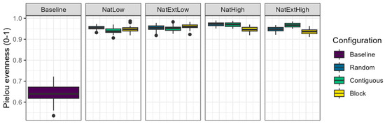
Figure 4.
Evenness in scaled landscape performance indicators across baseline and restored virtual landscapes. Box and whisker plots show the median (bold line), interquartile range (box), and range within 1.5 × IQR (whiskers). NatLow = natural restoration low with no extensive grassland; NatHigh = natural restoration high with no extensive grassland; NatExtLow = natural restoration low with additional extensive grassland target; NatExtHigh = natural restoration high with additional extensive grassland target.
The average mean scaled score provided by each land cover varied significantly depending on the restored area, restoration of extensive grassland, and configuration (Supplementary Figures S19–S24, Supplementary Table S5). The multifunctionality of each land cover showed contrasting patterns for different land covers, reflecting the effects that the land cover types have in the underlying indicator models. For example, the mean scaled score within cropland typically increased in the restoration realisations as compared to the baseline and was highest in realisations with the random restoration configuration (Supplementary Figure S19). This was largely driven by the pollination indicator because a greater proportion of cropland is likely to be successfully pollinated when the area of pollinator-supporting land covers is greater and when pollinator habitats are distributed evenly across the landscape (Supplementary Figure S14). As another example, the mean scaled score within the exotic forest increased in the restored realisations and was highest in realisations with the block restoration configuration (Supplementary Figure S23). This was largely driven by the kererū and kiwi biodiversity indicators, which gave a greater connected area of suitable habitat when large blocks were restored, and by the recreation indicator, which awards a higher recreational opportunity score to large blocks of natural forest (Supplementary Figures S15–S18). Conversely, the mean scaled score within scrub and extensive grassland declined in some restored realisations when compared to the baseline (Supplementary Figures S21 and S22). This is due to the restored patches being, on average, smaller than the baseline patches of these habitats, thus slightly reducing the performance for the bird biodiversity and recreational opportunity indicators (Supplementary Figures S4 and S5, Supplementary Table S2). The mean scaled score provided by most land cover types was significantly different between the high and low restored area treatments, indicating that their average multifunctionality is impacted by the area restored (Supplementary Table S5). The mean scaled score was significantly higher with greater restored area in the crop, intensive grassland, exotic forest, and natural forest land cover types and was significantly lower in the extensive grasslands with greater restored area (Supplementary Figures S19–S24, Supplementary Table S5).
4. Discussion
4.1. Interactions between Restoration Composition and Configuration
Our simulation is the first virtual landscape experiment to test the relative and combined effects of different restoration strategies on ecosystem services, agricultural profit, biodiversity, and multifunctionality within intensive production landscapes. We found significant interaction effects between landscape configuration and the restored area for many indicators, as well as for multifunctionality and evenness. The configuration of restoration interventions not only directly impacted the outcomes but also modified the benefits of the restored area, supporting the suggestion that restoration needs to be approached with an understanding of whole landscape interactions and emergent properties [79]. Restoration of intensive production landscapes must, therefore, consider not only the amount of natural vegetation to restore but also the spatial arrangement of restoration interventions across the landscape [16]. The spatial design of landscape conservation and restoration has previously focused on biodiversity or species conservation outcomes, so it has generally recommended approaches that extend and connect existing areas and result in larger patches of natural habitat [31,32,33,80]. Among our three restoration approaches, the block configuration generally gave the largest connected areas of natural and semi-natural vegetation cover and thus performed best for the biodiversity indicators (Supplementary Figures S16 and S17). However, different spatial configurations benefited other ecosystem services—for example, pollination and nitrogen retention performance were highest under the random configuration realisations (Supplementary Figures S13 and S14). The random spatial configuration scored highly for these indicators because of their reliance on adjacencies between different land cover types; in the case of pollination, it scored high because crops must be located within foraging distance from suitable pollinator habitats [26,81,82], and in the case of nitrogen, it scored high retention because land covers with high retention capacity must be located downstream of land covers with high nitrogen loads [66]. Thus, depending on the prioritisation that restoration planners and stakeholders in a specific landscape place on different ecosystem services and components of biodiversity, the best-performing spatial restoration configuration may vary, not just the best-performing land cover composition [3,83].
The addition of extensive grassland restoration alongside natural forest and scrub restoration generally provided a small increase in performance for the ecosystem service and biodiversity indicators, with more substantial improvements for reducing greenhouse gas emissions and soil erosion. The benefits from restoring extensive grassland also depended on configuration and on the total restored area, with greater benefits from block or contiguous as compared to random restoration (Supplementary Figure S21). Extensive grassland supports many ecosystem services and aspects of biodiversity, although typically does not quite match the performance of natural forests [45]. However, extensive grassland may play an important role in future landscape restoration due to its capacity to support some ecosystem services [3,9] and enhance the benefits of natural woody vegetation. Furthermore, extensive grassland may be a socially acceptable addition to restoring natural forest and scrub because extensive grasslands can simultaneously provide pastoral grazing for lower-intensity livestock, thus maintaining some economic production [3,18,84]. For landscapes where it is difficult to reach substantial coverage of natural forest, it may, therefore, be possible to implement some extensive grassland restoration as a complement to smaller natural forest restoration efforts. Furthermore, our simulations suggest that strategic placement of extensive grassland adjacent to existing natural and semi-natural vegetation or in large contiguous blocks may support higher multifunctionality within the extensive grasslands themselves.
The restoration realisations performed differently for their overall landscape multifunctionality, and these patterns were partly driven by differences in the mean scaled score provided by different land covers (particularly natural forests). The overall mean scaled score and mean scaled scores for crops, exotic forests, and natural forests increased under the greater restored area treatments, indicating that more ambitious restoration strategies can enhance the performance of land covers—thus providing gains in multifunctionality additional to the effects of increasing restored area alone. The multifunctionality provided at a specific location is influenced by the characteristics of its surroundings, and this context-dependence is important when considering restoration planning at the sub-landscape scale. In reality, restoration interventions will commonly develop from bottom–up initiatives by individuals and groups and will therefore not be planned at the landscape scale to meet specific land cover area and configuration objectives [29,30]. For bottom–up restoration of natural forests, spatial targeting could help to maximise the benefit of restoring a fixed area by matching the location to optimise adjacency and patch size benefits [85].
Designing a restoration scheme for an existing landscape is different from designing a novel landscape because the baseline situation also impacts how proposed changes will propagate. In our virtual landscapes, restoration configuration significantly altered the total carbon stock and agricultural profit provided by a landscape because the configuration strategies differentially replaced the human-dominated land cover types. When planning the configuration of restoration interventions, it is therefore important to consider not only the desirable spatial patterns for providing ecosystem services and supporting biodiversity but also the interactions with existing land cover for decision-making [86,87].
Restoring natural woody vegetation and extensive grassland has an economic cost, notably the opportunity cost associated with converting productive agricultural land (de Souza et al. 2021). Correspondingly, in our simulation, the profit from agricultural production was substantially reduced across all restored scenarios due to the conversion of highly profitable crops and intensive grassland to less profitable land covers (Supplementary Figure S18). It is established that landscape-scale ecological restoration will have negative impacts on agricultural production, but these impacts may be compensated at the level of individual landowners by government subsidies or through profits from non-agricultural land uses such as carbon trading or tourism [41]. We did not model income from these ecosystem services in this case due to uncertainties about the potential for tourism in our virtual landscapes and the New Zealand carbon price. However, there is potential that at least some of the lost agricultural production in restored landscapes may be offset through alternative economic mechanisms.
4.2. Virtual Landscapes as a Tool for Informing Restoration Principles
Virtual landscape simulations provide a generalising perspective and have previously been used to explore how variation in landscape characteristics, such as composition, patch size, and heterogeneity, impact ecosystem service provision and multifunctionality [26,50,51]. Our results demonstrate the additional value of virtual landscape simulations in exploring interactions between different landscape characteristics—in this case, how restoration strategies interact and combine to impact the landscape performance of restored intensive production landscapes. The virtual landscape approach allowed us to generate combinations of different restoration strategies with controlled characteristics and replicate these restoration strategies across landscapes that conformed precisely to the same landscape generation rules (the replicates had distinct but highly similar topographic types, land covers, and configurations). The ability to precisely control these variables is unique to virtual landscapes and could not have been achieved by comparing or manipulating real landscapes. Through the virtual landscape approach, we first described how individual indicators responded to interactions between different restoration treatments and analysed how these differing responses gave rise to emergent patterns in multifunctionality and evenness. This mechanistic understanding will be critical to developing restoration templates and strategies that lead to climate-smart outcomes [26,88].
Restoration of landscapes is a complex process involving numerous human decisions made by a diverse network of stakeholders with different interests and priorities [27,28,89]. Furthermore, restoration does not happen instantaneously but develops along pathways that can be unpredictable and liable to change over time with changing societal conditions and external pressures [90]. Our simulation to set restoration targets implicitly assumes that it will be possible to establish natural woody vegetation and extensive grassland ecosystems and that the restored ecosystems will have an equivalent ecosystem service performance to their counterparts present in the baseline landscapes. However, challenges in establishing trees mean that the eventual land cover may differ from the restoration plan, and restored ecosystems commonly do not match their undisturbed counterparts in supporting ecosystem services [27,36,50]. Representing the socio-ecological nature of landscapes and their temporal dynamism requires a more detailed representation of people within virtual landscape models. Our generation of virtual landscapes innovated upon previous work by implementing a binary space partitioning method to represent the grid patterns of land use that commonly develop in human-dominated parts of the landscape [52], and this grid pattern represented human land ownership and decision-making when generating the restored realisations. To further represent the complexity of human decision-making within virtual landscapes, agent-based models or Bayesian networks could be used to represent the dynamic nature of land use change decisions in response to objectives or changing external drivers [87,91,92].
4.3. Towards General Guidelines for Restoring Landscapes
Restoring natural forest, scrub, and extensive grassland in intensive production landscapes restored multifunctionality and provided a more even suite of benefits, further enhanced by restoring larger areas. Most of the variation in multifunctionality was explained by the area of land restored, with additional extensive grassland restoration having a small but significant enhancement effect. The random spatial configuration provided the greatest multifunctionality. These findings are consistent with previous research and policy guidelines for the required area of native woody cover restoration, which has generally recommended a template of around 30% cover [6,16,17,18,19,20]. Furthermore, our findings support the argument that extensive grassland restoration can enhance the effects of forest restoration [3,9,18].
In contrast, the recommendation to target restoration interventions so that they are scattered across the landscape runs against prevailing advice to extend and connect existing habitat fragments areas and provide large patches of connected natural ecosystems [31,32,33,80]. This recommendation may also not match the realities of land use decisions, where it may be more feasible to alter marginal production land, which may be spatially clustered, or encourage interventions through social networks located in some regions [40,93]. As an alternative to following one of our idealised configuration strategies uniformly, it may be more feasible to combine these approaches to varying degrees across a landscape. This approach would provide heterogeneity in patch sizes and connectivity across the landscape, potentially allowing greater multifunctionality by segregating different functions in contrasting sub-regions [16,51]. Alternatively, it may be beneficial to follow a restoration strategy that directly targets increasing ecological connectivity across a landscape, for example, through implementing green infrastructure corridors that link natural habitats or woody vegetation fragments [94].
Our restoration planning recommendations may require modification to specific contexts and locations despite the virtual landscape approach aimed at identifying generalisable patterns. Our virtual landscapes were based on those found in Aotearoa, New Zealand, yet in intensive agriculture landscapes around the world, different vegetation types exist, and the parameterisation of the ecosystem service models may be different. Multifunctionality scores are influenced by the selection and importance weighting of the individual component indicators [60,95]. Our indicators were selected to represent key ecosystem services and elements of biodiversity that are considered important in intensive production landscapes in Aotearoa, New Zealand, but represent different types of benefits to human well-being and a combination of spatially sensitive and spatially insensitive models [26]. Furthermore, our indicators include many of those that are considered important in intensive production landscapes around the world [96,97]. Perhaps more critical than the selection of indicators is the relative importance that stakeholders place upon them in a particular landscape [83]. For our virtual landscapes, we assumed that all indicators have an equal importance in contributing to multifunctionality and that this was scaled against the range of provisions encountered across all realisations. In reality, some indicators will be prioritised above others, and stakeholders may consider that sufficient functionality is provided at different levels [60]. The weighting and thresholding of the indicators will influence the multifunctionality and evenness performance and, in turn, the effects of restoration. For example, if biodiversity is of key importance to stakeholders, the biodiversity indicators may receive a stronger weighting, which may result in multifunctionality being favoured by the contiguous or block configurations. To apply these templates when designing restoration strategies for real landscapes, it is therefore important to include participatory processes and further modelling to tailor the design to local specificities [98,99].
5. Conclusions
Restoring multifunctionality to intensive production landscapes is challenging due to their inherent socio-ecological complexity and conflicting pressures and drivers. In this study, abstracting some complexities through virtual landscape modelling helped quantify the relative performance of different restoration strategies if pursued in isolation, as well as their combined nonlinear effects. We found that restoring natural vegetation cover to intensive production landscapes can enhance biodiversity, ecosystem services and multifunctionality. Restoring a larger area of the landscape provided greater overall multifunctionality and enhanced the multifunctional contributions of natural forests. Furthermore, the restoration of extensive grassland enhanced the return on efforts from restoring the same area of natural forest and scrub, which may provide a socially acceptable pathway to supplementing woody restoration. It is critical to target the spatial configuration of restoration to the desired ecosystem service or biodiversity outcomes, as different spatial configurations modify the impacts of the area restored and the addition of extensive grassland.
Supplementary Materials
The following supporting information can be downloaded at https://www.mdpi.com/article/10.3390/land13040460/s1.
Author Contributions
Conceptualization, D.R. and S.L.; methodology, D.R., T.R.E., A.H. and S.L.; formal analysis, D.R. and T.R.E.; writing—original draft preparation, D.R.; writing—review and editing, D.R., T.R.E., A.H. and S.L. All authors have read and agreed to the published version of the manuscript.
Funding
This work was supported by the Strategic Science Investment Funding for Crown Research Institutes from the New Zealand Ministry of Business, Innovation and Employment’s Science and Innovation Group.
Data Availability Statement
The simulated virtual landscapes are available through the following Figshare repository—DOI: 10.6084/m9.figshare.25545847.
Conflicts of Interest
The authors declare no conflicts of interest.
References
- Goldewijk, K.K.; Beusen, A.; Van Drecht, G. The HYDE 3.1 Spatially Explicit Database of Human-Induced Global Land-Use Change over the Past 12,000 Years. Glob. Ecol. Biogeogr. 2011, 20, 73–86. [Google Scholar] [CrossRef]
- Song, X.; Hansen, M.C.; Stephen, V.; Peter, V.; Tyukavina, A.; Vermote, E.F.; Townshend, J.R. Global Land Change from 1982 to 2016. Nature 2018, 560, 639–643. [Google Scholar] [CrossRef]
- Bardgett, R.D.; Bullock, J.M.; Lavorel, S.; Manning, P.; Schaffner, U.; Ostle, N.; Chomel, M.; Durigan, G.; Fry, E.L.; Johnson, D.; et al. Combatting Global Grassland Degradation. Nat. Rev. Earth Environ. 2021, 2, 720–735. [Google Scholar] [CrossRef]
- Rey Benayas, J.M.; Bullock, J.M. Restoration of Biodiversity and Ecosystem Services on Agricultural Land. Ecosystems 2012, 15, 883–899. [Google Scholar] [CrossRef]
- Landis, D.A. Designing Agricultural Landscapes for Biodiversity-Based Ecosystem Services. Basic Appl. Ecol. 2017, 18, 1–12. [Google Scholar] [CrossRef]
- Garibaldi, L.A.; Oddi, F.J.; Miguez, F.E.; Bartomeus, I.; Orr, M.C.; Jobbágy, E.G.; Kremen, C.; Schulte, L.A.; Hughes, A.C.; Bagnato, C.; et al. Working Landscapes Need at Least 20% Native Habitat. Conserv. Lett. 2021, 14, e12773. [Google Scholar] [CrossRef]
- Scherr, S.J.; Shames, S.; Friedman, R. From Climate-Smart Agriculture to Climate-Smart Landscapes. Agric. Food Soc. 2012, 1, 12. [Google Scholar] [CrossRef]
- Harvey, C.A.; Chac, M.; Donatti, C.I.; Garen, E.; Hannah, L.; Andrade, A.; Bede, L.; Brown, D.; Calle, A.; Char, J.; et al. Climate-Smart Landscapes: Opportunities and Challenges for Integrating Adaptation and Mitigation in Tropical Agriculture. Conserv. Lett. 2014, 7, 77–90. [Google Scholar] [CrossRef]
- Lavorel, S.; Colloff, M.J.; Mcintyre, S.; Doherty, M.D.; Murphy, H.T.; Metcalfe, D.J.; Dunlop, M.; Williams, R.J.; Wise, R.M.; Williams, K.J. Ecological Mechanisms Underpinning Climate Adaptation Services. Glob. Change Biol. 2015, 21, 12–31. [Google Scholar] [CrossRef]
- Colloff, M.J.; Wise, R.M.; Palomo, I.; Lavorel, S.; Pascual, U. Nature’s Contribution to Adaptation: Insights from Examples of the Transformation of Social-Ecological Systems. Ecosyst. People 2020, 16, 137–150. [Google Scholar] [CrossRef]
- Orwin, K.H.; Mason, N.W.H.; Berthet, E.T.; Grelet, G.; Mudge, P.; Lavorel, S. Integrating Design and Ecological Theory to Achieve Adaptive Diverse Pastures. Trends Ecol. Evol. 2022, 37, 861–871. [Google Scholar] [CrossRef] [PubMed]
- Valdés, A.; Lenoir, J.; De Frenne, P.; Andrieu, E.; Chabrerie, O.; Cousins, S.A.O.; Deconchat, M.; De, P.; Diekmann, M.; Valdés, A.; et al. High Ecosystem Service Delivery Potential of Small Woodlands in Agricultural Landscapes. J. Appl. Ecol. 2020, 57, 4–16. [Google Scholar] [CrossRef]
- Case, B.S.; Pannell, J.L.; Stanley, M.C.; Norton, D.A.; Brugman, A.; Funaki, M.; Mathieu, C.; Songling, C.; Suryaningrum, F.; Buckley, H.L. The Roles of Non-Production Vegetation in Agroecosystems: A Research Framework for Filling Process Knowledge Gaps in a Social-Ecological Context. People Nat. 2020, 2, 292–304. [Google Scholar] [CrossRef]
- Tscharntke, T.; Grass, I.; Wanger, T.C.; Westphal, C.; Batáry, P. Beyond Organic Farming—Harnessing Biodiversity-Friendly Landscapes. Trends Ecol. Evol. 2021, 36, 919–930. [Google Scholar] [CrossRef] [PubMed]
- Grass, I.; Loos, J.; Baensch, S.; Batáry, P.; Librán-Embid, F.; Ficiciyan, A.; Klaus, F.; Riechers, M.; Rosa, J.; Tiede, J.; et al. Land-Sharing/-Sparing Connectivity Landscapes for Ecosystem Services and Biodiversity Conservation. People Nat. 2019, 1, 262–272. [Google Scholar] [CrossRef]
- Arroyo-Rodríguez, V.; Fahrig, L.; Tabarelli, M.; Watling, J.I.; Tischendorf, L.; Benchimol, M.; Cazetta, E.; Faria, D.; Leal, I.R.; Melo, F.P.L.; et al. Designing Optimal Human-Modified Landscapes for Forest Biodiversity Conservation. Ecol. Lett. 2020, 23, 1404–1420. [Google Scholar] [CrossRef] [PubMed]
- Díaz, S.; Zafra-Calvo, N.; Purvis, A.; Verburg, P.H.; Obura, D.; Leadley, P.; Chaplin-Kramer, R.; De Meester, L.; Dulloo, E.; Martín-López, B.; et al. Set Ambitious Goals for Biodiversity and Sustainability. Science 2020, 370, 411–413. [Google Scholar] [CrossRef]
- Smith, F.P.; Prober, S.M.; House, A.P.N.; McIntyre, S. Maximizing Retention of Native Biodiversity in Australian Agricultural Landscapes-The 10:20:40:30 Guidelines. Agric. Ecosyst. Environ. 2013, 166, 35–45. [Google Scholar] [CrossRef]
- European Commission. New EU Forest Strategy for 2030; European Commission: Brussels, Belgium, 2021. [Google Scholar]
- Government of India. National Forest Policy; Government of India: New Delhi, India, 1988.
- Mitchell, M.G.E.; Suarez-Castro, A.F.; Martinez-Harms, M.; Maron, M.; McAlpine, C.; Gaston, K.J.; Johansen, K.; Rhodes, J.R. Reframing Landscape Fragmentation’s Effects on Ecosystem Services. Trends Ecol. Evol. 2015, 30, 190–198. [Google Scholar] [CrossRef]
- Verhagen, W.; Van Teeffelen, A.J.A.; Baggio, A.; Poggio, L.; Gimona, A.; Verburg, P.H. Effects of Landscape Configuration on Mapping Ecosystem Service Capacity: A Review of Evidence and a Case Study in Scotland. Landsc. Ecol. 2016, 31, 1457–1479. [Google Scholar] [CrossRef]
- Qiu, J.; Turner, M.G. Importance of Landscape Heterogeneity in Sustaining Hydrologic Ecosystem Services in an Agricultural Watershed. Ecosphere 2015, 6, 1–19. [Google Scholar] [CrossRef]
- Cordingley, J.E.; Newton, A.C.; Rose, R.J.; Clarke, R.T.; Bullock, J.M. Can Landscape-Scale Approaches to Conservation Management Resolve Biodiversity-Ecosystem Service Trade-Offs? J. Appl. Ecol. 2016, 53, 96–105. [Google Scholar] [CrossRef]
- Prestele, R.; Verburg, P.H. The Overlooked Spatial Dimension of Climate-Smart Agriculture. Glob. Change Biol. 2020, 26, 1045–1054. [Google Scholar] [CrossRef]
- Lavorel, S.; Grigulis, K.; Richards, D.R.; Etherington, T.R.E.; Law, R.M.; Herzig, A. Templates for Multifunctional Landscape Design. Landsc. Ecol. 2022, 37, 913–934. [Google Scholar] [CrossRef]
- Mason, N.W.H.; Wiser, S.K.; Richardson, S.J.; Thorsen, M.J.; Holdaway, R.J.; Dray, S.; Thomson, F.J.; Carswell, F.E. Functional Traits Reveal Processes Driving Natural Afforestation at Large Spatial Scales. PLoS ONE 2013, 8, e75219. [Google Scholar] [CrossRef] [PubMed]
- Cortina-Segarra, J.; García-Sánchez, I.; Grace, M.; Andrés, P.; Baker, S.; Bullock, C.; Decleer, K.; Dicks, L.V.; Fisher, J.L.; Frouz, J.; et al. Barriers to Ecological Restoration in Europe: Expert Perspectives. Restor. Ecol. 2021, 29, e13346. [Google Scholar] [CrossRef]
- Fullerton, A.H.; Steel, E.A.; Lange, I.; Caras, Y. Effects of Spatial Pattern and Economic Uncertainties on Freshwater Habitat Restoration Planning: A Simulation Exercise. Restor. Ecol. 2010, 18, 354–369. [Google Scholar] [CrossRef]
- Coombes, B.L. Ecospatial Outcomes of Neoliberal Planning: Habitat Management in Auckland Region, New Zealand. Environ. Plan. B Plan. Des. 2003, 30, 201–218. [Google Scholar] [CrossRef]
- Lamichhane, B.R.; Persoon, G.A.; Leirs, H.; Poudel, S.; Subedi, N.; Pokheral, C.P.; Bhattarai, S.; Gotame, P.; Mishra, R.; de Iongh, H.H. Contribution of Buffer Zone Programs to Reduce Human-Wildlife Impacts: The Case of the Chitwan National Park, Nepal. Hum. Ecol. 2019, 47, 95–110. [Google Scholar] [CrossRef]
- Digiovinazzo, P.; Ficetola, G.F.; Bottoni, L.; Andreis, C.; Padoa-Schioppa, E. Ecological Thresholds in Herb Communities for the Management of Suburban Fragmented Forests. For. Ecol. Manag. 2010, 259, 343–349. [Google Scholar] [CrossRef]
- Schultz, C.B.; Crone, E.E. Patch Size and Connectivity Thresholds for Butterfly Habitat Restoration. Conserv. Biol. 2005, 19, 887–896. [Google Scholar] [CrossRef]
- Fahrig, L.; Arroyo-Rodríguez, V.; Bennett, J.R.; Boucher-Lalonde, V.; Cazetta, E.; Currie, D.J.; Eigenbrod, F.; Ford, A.T.; Harrison, S.P.; Jaeger, J.A.G.; et al. Is Habitat Fragmentation Bad for Biodiversity? Biol. Conserv. 2019, 230, 179–186. [Google Scholar] [CrossRef]
- Meli, P.; Rey-Benayas, J.M.; Brancalion, P.H.S. Balancing Land Sharing and Sparing Approaches to Promote Forest and Landscape Restoration in Agricultural Landscapes: Land Approaches for Forest Landscape Restoration. Perspect. Ecol. Conserv. 2019, 17, 201–205. [Google Scholar] [CrossRef]
- Barral, M.P.; Rey Benayas, J.M.; Meli, P.; Maceira, N.O. Quantifying the Impacts of Ecological Restoration on Biodiversity and Ecosystem Services in Agroecosystems: A Global Meta-Analysis. Agric. Ecosyst. Environ. 2015, 202, 223–231. [Google Scholar] [CrossRef]
- Stott, I.; Soga, M.; Inger, R.; Gaston, K.J. Land Sparing Is Crucial for Urban Ecosystem Services. Front. Ecol. Environ. 2015, 13, 387–393. [Google Scholar] [CrossRef]
- Saunders, C. Conservation Covenants in New Zealand. Land Use Policy 1996, 13, 325–329. [Google Scholar] [CrossRef]
- Adams, W.M.; Hodge, I.D.; Macgregor, N.A.; Sandbrook, L.C. Creating Restoration Landscapes: Partnerships in Large-Scale Conservation in the UK. Ecol. Soc. 2016, 21, 1. [Google Scholar] [CrossRef]
- Yletyinen, J.; Perry, G.L.W.; Brown, P.; Pech, R.; Tylianakis, J.M. Multiple Social Network Influences Can Generate Unexpected Environmental Outcomes. Sci. Rep. 2021, 11, 9768. [Google Scholar] [CrossRef]
- Westerink, J.; Jongeneel, R.; Polman, N.; Prager, K.; Franks, J.; Dupraz, P.; Mettepenningen, E. Collaborative Governance Arrangements to Deliver Spatially Coordinated Agri-Environmental Management. Land Use Policy 2017, 69, 176–192. [Google Scholar] [CrossRef]
- Thomas, A.; Masante, D.; Jackson, B.; Cosby, B.; Emmett, B.; Jones, L. Fragmentation and Thresholds in Hydrological Flow-Based Ecosystem Services. Ecol. Appl. 2020, 30, e02046. [Google Scholar] [CrossRef]
- Gao, X.; Wang, J.; Li, C.; Shen, W.; Song, Z.; Nie, C.; Zhang, X. Land Use Change Simulation and Spatial Analysis of Ecosystem Service Value in Shijiazhuang under Multi-Scenarios. Environ. Sci. Pollut. Res. 2021, 28, 31043–31058. [Google Scholar] [CrossRef] [PubMed]
- Shoemaker, D.A.; BenDor, T.K.; Meentemeyer, R.K. Anticipating Trade-Offs between Urban Patterns and Ecosystem Service Production: Scenario Analyses of Sprawl Alternatives for a Rapidly Urbanizing Region. Comput. Environ. Urban Syst. 2019, 74, 114–125. [Google Scholar] [CrossRef]
- Gómez-Creutzberg, C.; Lagisz, M.; Nakagawa, S.; Brockerhoff, E.G.; Tylianakis, J.M. Consistent Trade-Offs in Ecosystem Services between Land Covers with Different Production Intensities. Biol. Rev. 2021, 96, 1989–2008. [Google Scholar] [CrossRef] [PubMed]
- Hanisch, M.; Schweiger, O.; Cord, A.F.; Volk, M.; Knapp, S. Plant Functional Traits Shape Multiple Ecosystem Services, Their Trade-Offs and Synergies in Grasslands. J. Appl. Ecol. 2020, 57, 1535–1550. [Google Scholar] [CrossRef]
- Oberlack, C.; Sietz, D.; Bonanomi, E.B.; De Bremond, A.; Dell’ Angelo, J.; Eisenack, K.; Ellis, E.C.; David, M.; Giger, M.; Heinimann, A.; et al. Archetype Analysis in Sustainability Research: Meanings, Motivations, and Evidence-Based Policy Making. Ecol. Soc. 2019, 24, 26. [Google Scholar] [CrossRef]
- Fiedler, S.; Monteiro, J.A.F.; Hulvey, K.B.; Standish, R.J.; Perring, M.P.; Tietjen, B. Global Change Shifts Trade-Offs among Ecosystem Functions in Woodlands Restored for Multifunctionality. J. Appl. Ecol. 2021, 58, 1705–1717. [Google Scholar] [CrossRef]
- Vallet, A.; Locatelli, B.; Levrel, H.; Wunder, S.; Seppelt, R.; Scholes, R.J.; Oszwald, J. Relationships Between Ecosystem Services: Comparing Methods for Assessing Tradeoffs and Synergies. Ecol. Econ. 2018, 150, 96–106. [Google Scholar] [CrossRef]
- Richards, D.R.; Moggridge, H.L.; Maltby, L.; Warren, P.H. Impacts of Habitat Heterogeneity on the Provision of Multiple Ecosystem Services in a Temperate Floodplain. Basic Appl. Ecol. 2018, 29, 32–43. [Google Scholar] [CrossRef]
- van der Plas, F.; Allan, E.; Fischer, M.; Alt, F.; Arndt, H.; Binkenstein, J.; Blaser, S.; Blüthgen, N.; Böhm, S.; Hölzel, N.; et al. Towards the Development of General Rules Describing Landscape Heterogeneity–Multifunctionality Relationships. J. Appl. Ecol. 2019, 56, 168–179. [Google Scholar] [CrossRef]
- Etherington, T.R.; Morgan, F.J.; Sullivan, D.O. Binary Space Partitioning Generates Hierarchical and Rectilinear Neutral Landscape Models Suitable for Human-Dominated Landscapes. Landsc. Ecol. 2022, 37, 1761–1769. [Google Scholar] [CrossRef]
- Harris, C.R.; Millman, K.J.; van der Walt, S.J.; Gommers, R.; Virtanen, P.; Cournapeau, D.; Wieser, E.; Taylor, J.; Berg, S.; Smith, N.J.; et al. Array Programming with NumPy. Nature 2020, 585, 357–362. [Google Scholar] [CrossRef] [PubMed]
- Virtanen, P.; Gommers, R.; Oliphant, T.E.; Haberland, M.; Reddy, T.; Cournapeau, D.; Burovski, E.; Peterson, P.; Weckesser, W.; Bright, J.; et al. SciPy 1.0: Fundamental Algorithms for Scientific Computing in Python. Nat. Methods 2020, 17, 261–272. [Google Scholar] [CrossRef] [PubMed]
- Van Der Walt, S.; Schönberger, J.L.; Nunez-Iglesias, J.; Boulogne, F.; Warner, J.D.; Yager, N.; Gouillart, E.; Yu, T. Scikit-Image: Image Processing in Python. PeerJ 2014, 2, e453. [Google Scholar] [CrossRef] [PubMed]
- Etherington, T.R.; Holland, E.P.; O’Sullivan, D. NLMpy: A Python Software Package for the Creation of Neutral Landscape Models within a General Numerical Framework. Methods Ecol. Evol. 2015, 6, 164–168. [Google Scholar] [CrossRef]
- Open Source Geospatial Foundation GDAL/OGR Geospatial Data Abstraction Software Library 2020. Available online: https://gdal.org (accessed on 1 October 2022). [CrossRef]
- Barnes, R. RichDEM Terrain Analysis Software. 2020. Available online: http://github.com/r-barnes/richdem (accessed on 1 October 2022).
- Rojas, I.M.; Pidgeon, A.M.; Radeloff, V.C. Restoring Riparian Forests According to Existing Regulations Could Greatly Improve Connectivity for Forest Fauna in Chile. Landsc. Urban Plan. 2020, 203, 103895. [Google Scholar] [CrossRef]
- Hölting, L.; Beckmann, M.; Volk, M.; Cord, A.F. Multifunctionality Assessments—More than Assessing Multiple Ecosystem Functions and Services ? A Quantitative Literature Review. Ecol. Indic. 2019, 103, 226–235. [Google Scholar] [CrossRef]
- Duarte, G.T.; Mitchell, M.; Martello, F.; Gregr, E.J.; Paglia, A.P.; Chan, K.M.A.; Ribeiro, M.C. A User-Inspired Framework and Tool for Restoring Multifunctional Landscapes: Putting into Practice Stakeholder and Scientific Knowledge of Landscape Services. Landsc. Ecol. 2020, 35, 2535–2548. [Google Scholar] [CrossRef]
- Case, B.; Ryan, C. A Preliminary Analysis of Carbon Stocks and Net Carbon Position for New Zealand Sheep and Beef Farmland; Auckland University of Technology: Auckland, New Zealand, 2020. [Google Scholar]
- Paul, T.S.H.; Kimberley, M.O.; Beets, P.N. Carbon Stocks and Change in New Zealand’s Natural Forests; Estimates from the First Two Complete Inventory Cycles 2002–2007 and 2007–2014; New Zealand Forest Research Institute Limited: Rotorua, New Zealand, 2019. [Google Scholar]
- Thomas, S.; Ausseil, A.-G.; Guo, J.; Herzig, A.; Khaembah, E.; Palmer, D.; Renwick, A.; Teixeira, E.; van der Weerden, T.; Wakelin, S. Evaluation of Profitability and Future Potential for Low Emission Productive Uses of Land That Is Currently Used for Livestock SLMACC Project 405422; Department of Global Value Chains and Trade, Lincoln University: Canterbury, New Zealand, 2020. [Google Scholar]
- Dymond, J.R. Soil Erosion in New Zealand Is a Net Sink of CO2. Earth Surf. Process. Landf. 2010, 35, 1763–1772. [Google Scholar] [CrossRef]
- Sharp, R.; Tallis, H.T.; Ricketts, T.; Guerry, A.D.; Wood, S.A.; Chaplin-Kramer, R.; Nelson, E.; Ennaanay, D.; Wolny, S.; Olwero, N.; et al. InVEST 3.8.9. User’s Guide; The Natural Capital Project; Stanford University: Stanford, CA, USA; University of Minnesota: Minneapolis, MN, USA; The Nature Conservancy, and World Wildlife Fund: Gland, Switzerland, 2016. [Google Scholar]
- Stachelek, J. Rinvest: InVEST: Ecosystem Service and Valuation Models; R Package v 0.1; 2022. Available online: https://github.com/jsta/rinvest (accessed on 1 October 2022).
- Byczek, C.; Longaretti, P.Y.; Renaud, J.; Lavorel, S. Benefits of Crowd-Sourced GPS Information for Modelling the Recreation Ecosystem Service. PLoS ONE 2018, 13, e0202645. [Google Scholar] [CrossRef]
- Richards, D.R.; Lavorel, S. Integrating Social Media Data and Machine Learning to Analyse Scenarios of Landscape Appreciation. Ecosyst. Serv. 2022, 55, 101422. [Google Scholar] [CrossRef]
- Bal, P.; Tulloch, A.I.T.; Addison, P.F.E.; Mcdonald-madden, E.; Rhodes, J.R. Selecting Indicator Species for Biodiversity Management. Front. Ecol. Environ. 2018, 16, 589–598. [Google Scholar] [CrossRef]
- Lindenmayer, D.B.; Likens, G.E. Surrogate Indicator Species for Evaluating Environmental Change and Biodiversity Loss. Ecosystems 2011, 14, 47–59. [Google Scholar] [CrossRef]
- Zhang, J.; Pannell, J.L.; Case, B.S.; Hinchliffe, G.; Stanley, M.C.; Buckley, H.L. Interactions between Landscape Structure and Bird Mobility Traits Affect the Connectivity of Agroecosystem Networks. Ecol. Indic. 2021, 129, 107962. [Google Scholar] [CrossRef]
- Mestre, F.; Silva, B. Lconnect: Simple Tools to Compute Landscape Connectivity Metrics. 2021. Available online: https://CRAN.R-project.org/package=lconnect (accessed on 1 October 2022).
- McGarigal, K.; Marks, B.J. FRAGSTATS: Spatial Pattern Analysis Program for Quantifying Landscape Structure; General Technical Report; US Department of Agriculture, Forest Service, Pacific Northwest Research Station: Portland, OR, USA, 1995.
- Hesselbarth, M.H.K.; Sciaini, M.; With, K.A.; Wiegand, K.; Nowosad, J. Landscapemetrics: An Open-Source R Tool to Calculate Landscape Metrics. Ecography 2019, 42, 1648–1657. [Google Scholar] [CrossRef]
- Bates, D.; Mächler, M.; Bolker, B.M.; Walker, S.C. Fitting Linear Mixed-Effects Models Using Lme4. J. Stat. Softw. 2015, 67, 48. [Google Scholar] [CrossRef]
- Kuznetsova, A.; Brockhoff, P.B.; Christensen, R.H.B. LmerTest Package: Tests in Linear Mixed Effects Models. J. Stat. Softw. 2017, 82, 1–26. [Google Scholar] [CrossRef]
- Luke, S.G. Evaluating Significance in Linear Mixed-Effects Models in R. Behav. Res. Methods 2017, 49, 1494–1502. [Google Scholar] [CrossRef] [PubMed]
- Bullock, J.M.; Fuentes-Montemayor, E.; McCarthy, B.; Park, K.; Hails, R.S.; Woodcock, B.A.; Watts, K.; Corstanje, R.; Harris, J. Future Restoration Should Enhance Ecological Complexity and Emergent Properties at Multiple Scales. Ecography 2022, 2022, 1–11. [Google Scholar] [CrossRef]
- Ward, M.; Saura, S.; Williams, B.; Ramírez-Delgado, J.P.; Arafeh-Dalmau, N.; Allan, J.R.; Venter, O.; Dubois, G.; Watson, J.E.M. Just Ten Percent of the Global Terrestrial Protected Area Network Is Structurally Connected via Intact Land. Nat. Commun. 2020, 11, 4563. [Google Scholar] [CrossRef]
- Montoya, D.; Haegeman, B.; Gaba, S.; de Mazancourt, C.; Bretagnolle, V.; Loreau, M. Trade-Offs in the Provisioning and Stability of Ecosystem Services in Agroecosystems. Ecol. Appl. 2019, 29, e01853. [Google Scholar] [CrossRef]
- Maes, J.; Paracchini, M.L.; Zulian, G.; Dunbar, M.B.; Alkemade, R. Synergies and Trade-Offs between Ecosystem Service Supply, Biodiversity, and Habitat Conservation Status in Europe. Biol. Conserv. 2020, 155, 1–12. [Google Scholar] [CrossRef]
- Neyret, M.; Fischer, M.; Allan, E.; Hölzel, N.; Klaus, V.H.; Kleinebecker, T.; Krauss, J.; Le Provost, G.; Peter, S.; Schenk, N.; et al. Assessing the Impact of Grassland Management on Landscape Multifunctionality. Ecosyst. Serv. 2021, 52, 101366. [Google Scholar] [CrossRef]
- Abbott, M.; Boyle, C.; Lee, W.; Xuejing, L. Interweaving Protected Areas and Productive Landscapes in Aotearoa New Zealand: Using Design to Explore Multifunctionality in the Mackenzie Basin. J. Landsc. Archit. 2019, 14, 6–19. [Google Scholar] [CrossRef]
- de Souza, A.R.; Dupas, F.A.; da Silva, I.A. Spatial Targeting Approach for a Payment for Ecosystem Services Scheme in a Peri-Urban Wellhead Area in Southeastern Brazil. Environ. Chall. 2021, 5, 100206. [Google Scholar] [CrossRef]
- Plieninger, T.; Kizos, T.; Bieling, C.; Le Dû-Blayo, L.; Budniok, M.A.; Bürgi, M.; Crumley, C.L.; Girod, G.; Howard, P.; Kolen, J.; et al. Exploring Ecosystem-Change and Society through a Landscape Lens: Recent Progress in European Landscape Research. Ecol. Soc. 2015, 20, 5. [Google Scholar] [CrossRef]
- Bartkowski, B.; Beckmann, M.; Drechsler, M.; Kaim, A.; Liebelt, V.; Müller, B.; Witing, F.; Strauch, M. Aligning Agent-Based Modeling with Multi-Objective Land-Use Allocation: Identification of Policy Gaps and Feasible Pathways to Biophysically Optimal Landscapes. Front. Environ. Sci. 2020, 8, 103. [Google Scholar] [CrossRef]
- Wu, J. Landscape Sustainability Science (II): Core Questions and Key Approaches; Springer: Dordrecht, The Netherlands, 2021; ISBN 0123456789. [Google Scholar]
- Mansourian, S.; Parrotta, J.; Balaji, P.; Bellwood-Howard, I.; Bhasme, S.; Bixler, R.P.; Boedhihartono, A.K.; Carmenta, R.; Jedd, T.; de Jong, W.; et al. Putting the Pieces Together: Integration for Forest Landscape Restoration Implementation. Land Degrad. Dev. 2020, 31, 419–429. [Google Scholar] [CrossRef]
- Gillson, L.; Dirk, C.; Gell, P. Using Long-Term Data to Inform a Decision Pathway for Restoration of Ecosystem Resilience. Anthropocene 2021, 36, 100315. [Google Scholar] [CrossRef]
- Murray-Rust, D.; Brown, C.; van Vliet, J.; Alam, S.J.; Robinson, D.T.; Verburg, P.H.; Rounsevell, M. Combining Agent Functional Types, Capitals and Services to Model Land Use Dynamics. Environ. Model. Softw. 2014, 59, 187–201. [Google Scholar] [CrossRef]
- Bakker, M.M.; Alam, S.J.; van Dijk, J.; Rounsevell, M.D.A. Land-Use Change Arising from Rural Land Exchange: An Agent-Based Simulation Model. Landsc. Ecol. 2015, 30, 273–286. [Google Scholar] [CrossRef]
- West, T.A.P.; Monge, J.J.; Dowling, L.J.; Wakelin, S.J.; Yao, R.T.; Dunningham, A.G.; Payn, T. Comparison of Spatial Modelling Frameworks for the Identification of Future Afforestation in New Zealand. Landsc. Urban Plan. 2020, 198, 103780. [Google Scholar] [CrossRef]
- Simelton, E.; Carew-Reid, J.; Coulier, M.; Damen, B.; Howell, J.; Pottinger-Glass, C.; Tran, H.V.; Van Der Meiren, M. NBS Framework for Agricultural Landscapes. Front. Environ. Sci. 2021, 9, 678367. [Google Scholar] [CrossRef]
- Manning, P.; Van Der Plas, F.; Soliveres, S.; Allan, E.; Maestre, F.T.; Mace, G.; Whittingham, M.J.; Fischer, M. Redefining Ecosystem Multifunctionality. Nat. Ecol. Evol. 2018, 2, 427–436. [Google Scholar] [CrossRef] [PubMed]
- Kremen, C. Ecological Intensification and Diversification Approaches to Maintain Biodiversity, Ecosystem Services and Food Production in a Changing World. Emerg. Top. Life Sci. 2020, 4, 229–240. [Google Scholar] [CrossRef] [PubMed]
- Qiu, J.; Queiroz, C.; Bennett, E.M.; Cord, A.F.; Crouzat, E.; Lavorel, S.; Maes, J.; Meacham, M.; Norström, A.V.; Peterson, G.D.; et al. Land-Use Intensity Mediates Ecosystem Service Tradeoffs across Regional Social-Ecological Systems. Ecosyst. People 2021, 17, 264–278. [Google Scholar] [CrossRef]
- Campbell-Arvai, V.; Lindquist, M. From the Ground up: Using Structured Community Engagement to Identify Objectives for Urban Green Infrastructure Planning. Urban For. Urban Green. 2021, 59, 127013. [Google Scholar] [CrossRef]
- Do, T.H.; Vu, T.P.; Catacutan, D.; Nguyen, V.T. Governing Landscapes for Ecosystem Services: A Participatory Land-Use Scenario Development in the Northwest Montane Region of Vietnam. Environ. Manag. 2021, 68, 665–682. [Google Scholar] [CrossRef]
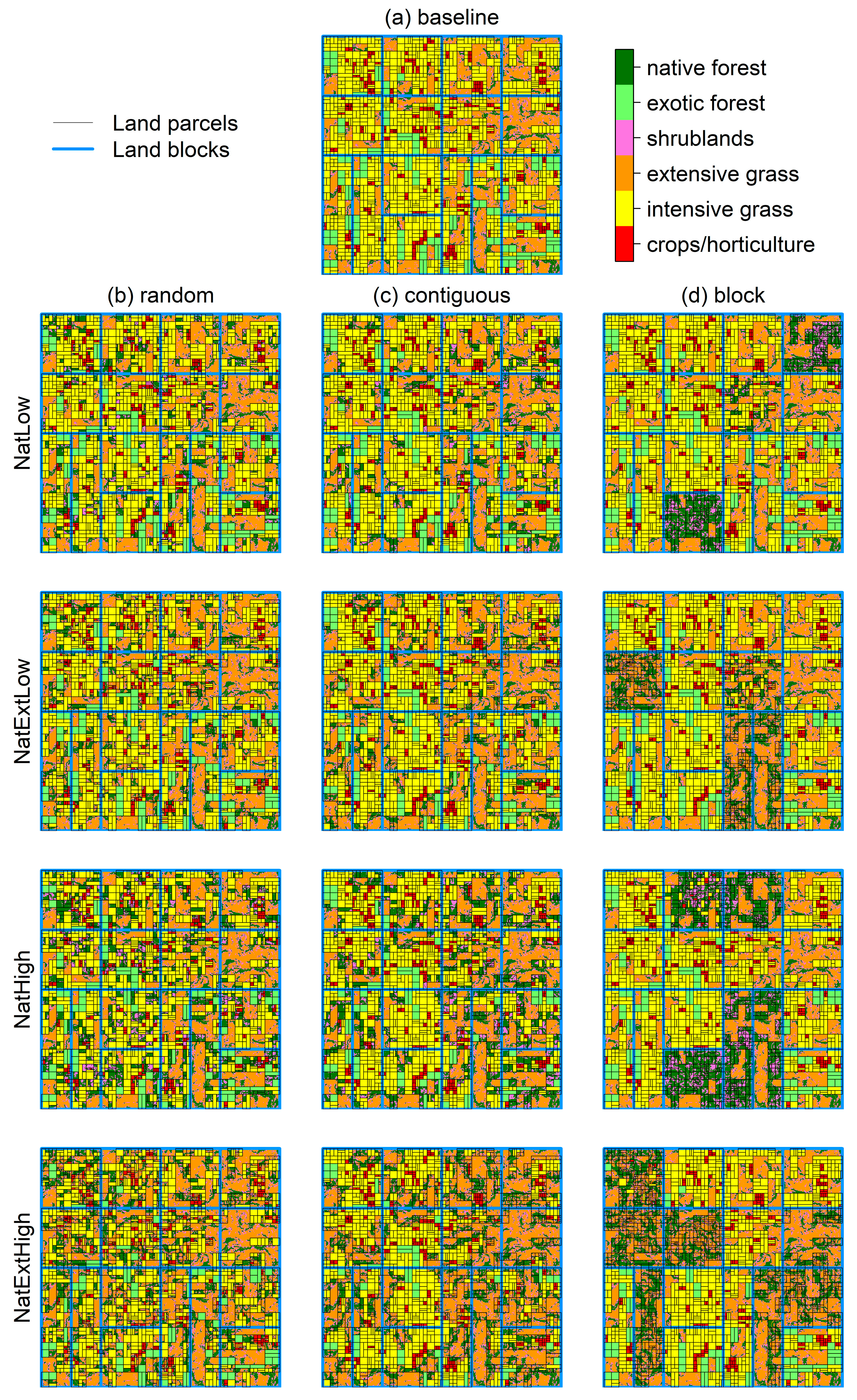
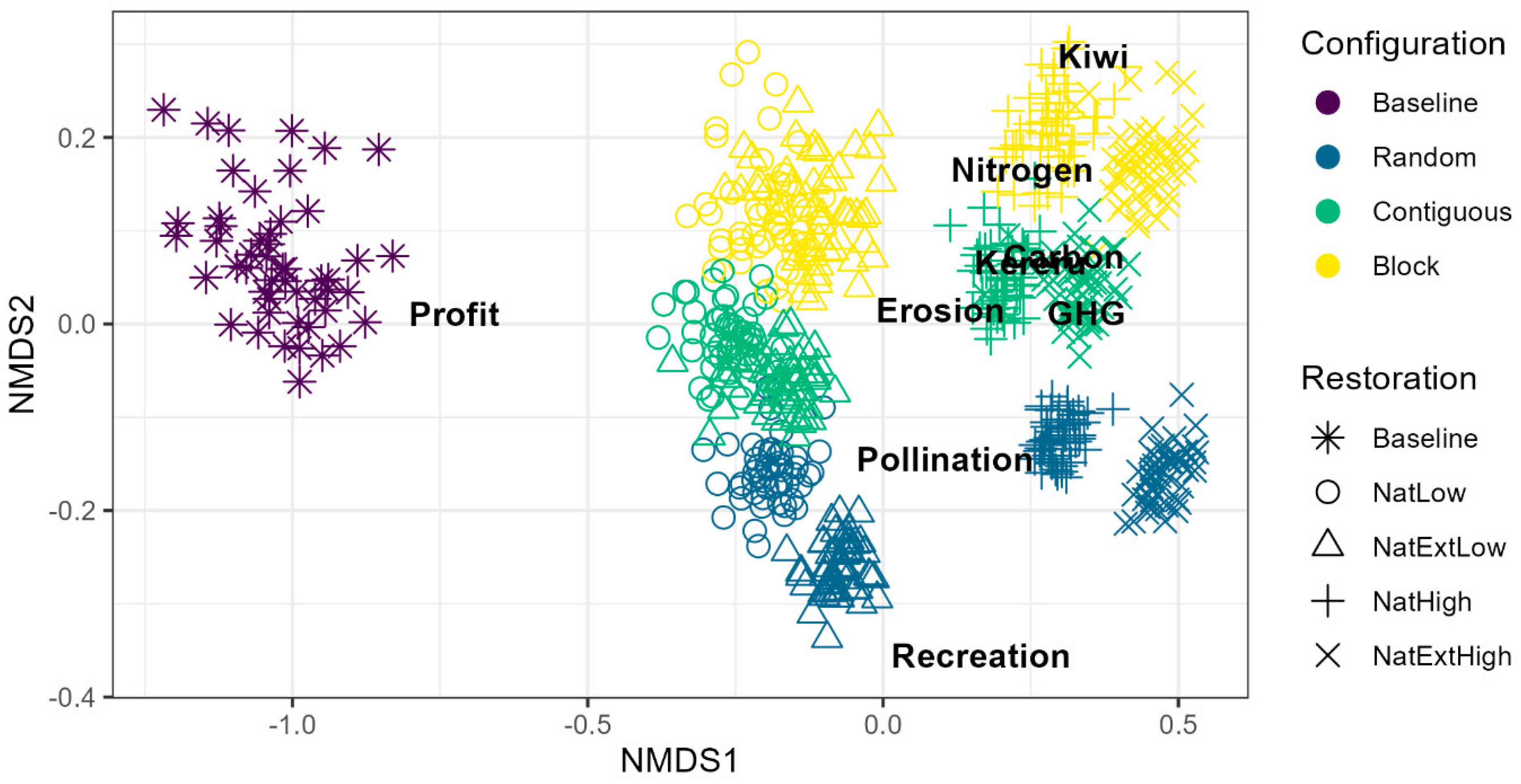
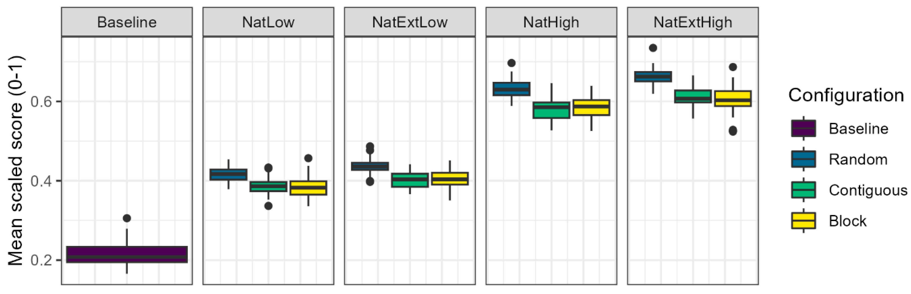

Disclaimer/Publisher’s Note: The statements, opinions and data contained in all publications are solely those of the individual author(s) and contributor(s) and not of MDPI and/or the editor(s). MDPI and/or the editor(s) disclaim responsibility for any injury to people or property resulting from any ideas, methods, instructions or products referred to in the content. |
© 2024 by the authors. Licensee MDPI, Basel, Switzerland. This article is an open access article distributed under the terms and conditions of the Creative Commons Attribution (CC BY) license (https://creativecommons.org/licenses/by/4.0/).