The Impact of Land-Use Mix on Technological Innovation: Evidence from a Grid-Cell-Level Analysis of Shanghai, China

Abstract

While the benefits of land-use mix have been widely analyzed with regard to transportation, public health, and economic development, relatively little attention has been paid to empirically investigating the impact of land-use mix on technological innovation at the intra-urban level. Drawing upon a database of geo-coded patents that are used to reflect the capacity of technological innovation, this paper takes Shanghai as a case study and analyzes how the intra-urban distribution of technological innovation has been associated with land-use mix at the 1 km × 1 km grid cell level. Empirical results, which are robust when the grids are divided at the 2 km × 2 km level, show that the degree of land-use mix is positively associated with the number of patents for a given grid, suggesting that grids with a higher level of land-use mix are likely to have more patents, ceteris paribus. Moreover, the results demonstrate an inverted U-curve relationship between land-use mix and technological innovation, indicating that a too much higher level of land-use mix could lead to a smaller number of patents for a certain grid. In addition, the empirical results suggest the existence of spatial dependence in the effect of land-use mix on technological innovation.

1. Introduction

Technological innovation is a complex process that is usually undertaken by entrepreneurs and knowledge workers and often involves the interplay of social, economic, and technological factors. With technological innovation playing an increasingly important role in promoting urban and regional development, much attention has been paid to investigating the determinants of the economic geography of technological innovation [1,2,3]. The traditional drivers of technological innovation that have been well documented in the literature generally include research and development (R&D) input [3,4,5], social and human capital [2,6,7,8], universities and research institutes [9,10,11], and external knowledge linkages [5,12,13]. While these studies have mainly focused on socioeconomic factors that could influence the geography of technological innovation, recent studies have also investigated the relationship between the geography of technological innovation and broadly defined built environment factors. For instance, some studies have found that the geography of technological innovation is associated with walkability [14,15] and the compactness of spatial structure [16,17] based on the empirical analyses of US cities. In the Chinese context, Li and Du showed a causal relationship between polycentric urban spatial structure and innovation capacity at the city level. Other things being equal, they found that Chinese cities with a lower degree of polycentricity tend to have higher innovation capacity [18]. Based on empirical evidence from China’s Pearl River Delta, Wu et al. showed that built environment factors, including a healthy environment, mixed land use, commuting convenience, and the technology atmosphere, all demonstrate significant impacts on regional innovation productivity [19]. In a recent case study on Nanjing, Li et al. found that technological innovation capacity is associated with the quantity and diversity of third places such as restaurants, parks, and coffee shops [20].

While the above-mentioned studies have contributed significantly to our understanding of the economic geography of technological innovation, most of these studies have been conducted at the urban and regional levels. We still know relatively little about the determinants of the intra-urban geography of technological innovation. At the intra-urban level, land-use mix is one of the most important components of the built environment that could influence the geography of technological innovation. In the field of urban planning, land-use mix usually refers to the variety and distribution of different types of land uses within a defined area, which could be a block, neighborhood, city, or region. Rather than focusing on a certain type of land use, it considers the degree of functional integration and spatial arrangement among different types of land uses (e.g., agricultural, residential, industrial, recreational, and commercial). The concept of land-use mix was put forward by Jacobs who suggested “mixed-use living spaces” in response to the increasingly serious problems caused by the “functional zoning” idea in traditional urban planning [21]. Driven by the rise of urban development strategies such as “smart growth” and “new urbanism” in the late 20th century, the concept of land-use mix has become increasingly popular among scholars, urban planners, and policymakers.

So far, a large number of studies have shown that land-use mix could generate many benefits, especially in the fields of transportation, public health, environmental sustainability, and urban economic development [22,23]. For instance, Pang et al. developed a bilevel model of mixed land use and transportation which shows that a mixed-land-use pattern could improve local traffic property [24]. Other studies have indicated that land-use mix could promote active travel modes such as walking and cycling and therefore reduce car dependence [12,25,26,27]. In terms of public health, land-use mix has been found to significantly account for people’s health indicators at the district level [28], which is mainly because a higher level of land-use mix could encourage people to walk for exercise and transportation [26,29]. With regard to environmental sustainability, O’Driscoll et al. argued that the efficiency of land use in Irish metropolitan areas has been relatively low, which is represented by a relatively lower degree of land-use mix. Furthermore, they argued that this inefficiency has been negatively associated with efforts made for environmental sustainability [30]. Finally, in terms of urban economic development, some studies have found that a diverse neighborhood represented by a higher degree of mixed land use tends to have higher property prices [31].

Although the benefits of land-use mix have been widely discussed from different perspectives, relatively little attention has been paid to empirically investigating the impacts of land-use mix on innovation capacity, especially at the intra-urban level. However, there are some notable exceptions that have examined the determinants of the intra-urban geography of technological innovation based on grid cell analyses, though these studies have not emphasized the role of land-use mix [19,20]. Here, we argue that land-use mix could influence technological innovation in at least three ways.

First, many studies have shown that the clustering of land with different functions within a defined area could improve the area’s attributes such as diversity, walkability, and service accessibility [22,26,29,32], which in theory all relate to technological innovation. For instance, according to Florida’s creative class theory, the creative class, whose professions span science, engineering, and design, have attached greater importance to a diversified, walkable, and accessible environment when choosing their living or work locations. Therefore, the above-mentioned distinct attributes have become increasingly important for an area to attract the creative class to live and work, thus facilitating the birth of new ideas, entrepreneurships, and new forms of businesses [11,33]. In addition, with the rise of innovation districts across the world, such attributes have been regarded as key aspects characterizing successful innovation districts [34]. For instance, some studies have argued that the success of Boston’s Kendall Square as one of the world’s most innovative areas has been largely due to the existence of walkable and bikeable places created by the mixed use of land with different functions [34,35]. In fact, the clustering of different types of land uses facilitates the provision of diverse services within close proximity. For instance, some studies have found that the commercialization of ideas and technology transfer could be accelerated by proximity to research institutions, incubators, and venture capital firms [4]. Some studies have also found that walkable environments promote physical activity and well-being, which are known to enhance cognitive function and creativity [14,15].

Second, the mixed use of land within a certain area is conducive to providing a convenient and livable environment, which could in turn make the area more attractive for enterprises to locate and knowledge workers to share and exchange tacit knowledge. With the innovation model of enterprises gradually changing from “closed innovation” to “open innovation” in the context of globalizing the knowledge economy, the exchange and flow of tacit knowledge have become increasingly important for enterprises and knowledge workers to stay innovative. However, unlike codified knowledge, tacit knowledge is hard to codify and can be mainly shared through face-to-face communications [36]. Studies have shown that face-to-face communications are particularly effective for sharing complex ideas, resolving conflicts, and generating creative solutions [34,35]. In this sense, areas with a higher level of land-use mix are more likely to facilitate geographical proximity between knowledge workers, thus providing more opportunities for face-to-face communications. In fact, by clustering diverse activities and amenities within walking distance, mixed land use could create opportunities for spontaneous encounters and serendipitous interactions among individuals from different backgrounds and professions [11,33].

Third, land-use mix could help build the social capital of neighborhoods, which is also conducive to facilitating the innovation process. For instance, Leyden showed that people tend to have a higher level of social capital if they live in a walkable and mixed-use neighborhood, indicating that land-use mix is positively associated with the development of social capital [37]. Importantly, mixed land use promotes the use of shared spaces and common amenities. Furthermore, many studies have documented the relationship between social capital and innovation [6,11]. For instance, Peiró-Palomino found that social capital plays an important role in the innovation process of 257 European regions, though the role differs across regions [6].

To fill in the above-mentioned research gap, this paper aims to empirically investigate the impact of land-use mix on the intra-urban geography of technological innovation. Specifically, this paper takes Shanghai as a case study and uses patents to reflect the capacity of technological innovation at the 1 km × 1 km grid cell level. The regression results show that grids with a higher level of land-use mix are likely to produce more patents, other things being equal. However, grids with a too much higher level of land-use mix are likely to have less patents, indicating that a threshold effect could exist in the impact of land-use mix on technological innovation. The results of spatial econometric regression models further show that grids are likely to have more patents if they are surrounded by grids with a larger number of patents, implying the existence of spatial dependence in the effect of land-use mix on technological innovation.

The remainder of this paper is structured as follows. The next section describes the research area, data, and methodology. Section 3 presents and discusses the empirical results of different regression models, which is followed by a discussion of policy implications in Section 4. Section 5 concludes with future research agendas.

2. Data and Methodology

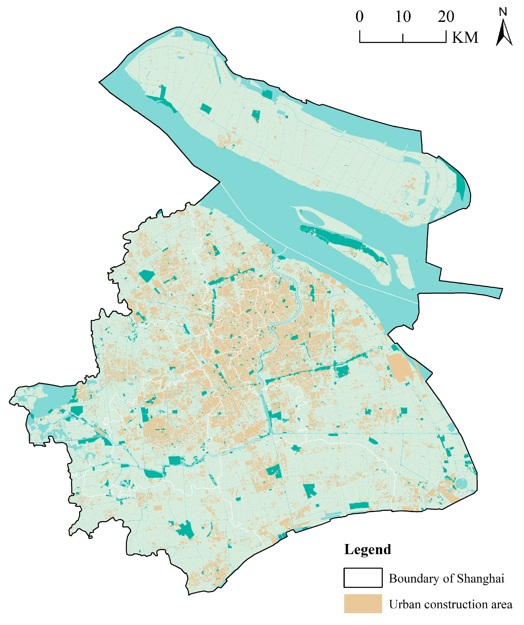
2.1. Research Area

This paper takes Shanghai as a case study, which is one of the most innovative cities in China. According to the 2023 Global Innovation Index, which was released by the World Intellectual Property Organization, the Shanghai-Suzhou cluster ranked fifth among the world’s top 100 science and technology clusters. As stated in its 14th Five-Year Plan for building a science and technology innovation center with global influence, Shanghai has aimed to improve its R&D intensity (i.e., the proportion of R&D expenditure to GDP) to 4.5% by 2025, striving to become a global leader in science and technology innovation. In addition, Shanghai has paid much attention to facilitating the mixed use of land. For instance, the municipal government of Shanghai has recently introduced a policy on comprehensively promoting the high-quality use of land resources, which encourages the mixed layout of land with different functions such as industrial, storage, research and development, office, and commercial use. Some studies have also measured and characterized the land-use mix patterns of Shanghai, showing that more than half of the sample streets have a relatively higher degree of land-use mix [38].

Taken together, we think that Shanghai could be an ideal case to investigate the impact of land-use mix on technological innovation, which, however, has gained relatively little attention among scholars and policymakers. We believe that the empirical results and policy implications derived from the case study of Shanghai could provide valuable experience for other cities that aim to improve their technological innovation capacity. In this paper, we define the research area as the total administrative area of Shanghai, which covers an area of about 6340 km² and is shown in Figure 1. Furthermore, we divide the research area into grid cells at approximately 1 km × 1 km level, which yields 11,408 grid cells in total. It should be noted that not all grid cells contain 1 km² land since many grids are at the fringe. Therefore, the number of grid cells is much higher than 6340. To test the robustness of the empirical results, we also divide the research area into grid cells at the 2 km × 2 km level based on the same criterion.

2.2. The Measurement of Land-Use Mix and Technological Innovation at the Grid Cell Level

While much attention has been paid to land-use mix, so far scholars have not reached a consensus on its definition, which has also affected the measurement of land-use mix. In a narrow sense, some scholars have defined land-use mix as the functional mixing of different types of urban buildable land [22,39]. However, in a broader sense, some scholars have argued that land-use mix should include the functional mixing of different types of facilities [40,41]. Furthermore, the geographical scale at which land-use mix is measured has also been found to account for the measurement of land-use mix [39]. In light of these different views, Song et al. identified the strengths and shortcomings of a variety of measures of land-use mix, providing suggestions about which measures of land-use mix should be applied at a given geographical scale or in a certain contextual situation [22]. Specifically, they divided the measures of land-use mix into integral measures and divisional measures. The former measures, which are only determined by the overall distribution of land-use types within a given area, usually include percentage, balance index, entropy index, and Herfindahl–Hirschman index. In contrast, the latter measures are sensitive to the patterns of land use, which often include Atkinson index, clustering index, and dissimilarity index (see Song et al. for detailed introduction). Furthermore, they proposed that the integral measures are suitable for situations where three or more types of land use are of interest and where the unit of analysis is at a relatively small scale.

Following the approach of Song et al., this paper mainly adopts the integral measures to calculate the degree of land-use mix at the grid cell level. Specifically, we use the entropy index, one of the most commonly used integral measures in the literature, to calculate the mixing degree of each grid’s land use. The expression is given as follows:

$${Mix}_i=-\frac{\left[{\sum }_{j=1}^k{P}_{ij}\ast Ln\left(P_{ij}\right)\right]}{Ln\left(k_i\right)}$$

(1)

where ${Mix}_i$ refers to the land-use mix degree of grid $i$, $P_{ij}$ is the percentage of each land-use type $j$ in grid $i$, and $k_i$ represents the total number of land-use types within the grid $i$. By definition, the value of ${Mix}_i$ ranges from 0 to 1, and the maximum value of ${Mix}_i$ can only be achieved when there is an even distribution of different types of land use.

In terms of the measurement of technological innovation, this paper uses the number of patents that each grid contains to reflect its capacity of technological innovation. Within the literature on the geography of innovation, patents have been widely used to reflect innovation capacity at different geographical scales [1,4,5]. However, we also bear in mind the shortcomings of using patents. For instance, not all innovation activities lead to patents, and the quality of patents varies across different sectors and technological fields [42]. Nonetheless, patents contain detailed information on applicants’ address, application year, technological classification, etc., which allows us to conduct spatial and comparable analyses. In this paper, since all the grids are of the same size, each grid’s technological innovation capacity represented by the number of patents that it contains is therefore comparable. It should be noted, however, that patent address may not accurately reflect the location where the patent invention was manufactured. In many cases, companies, especially multinational corporations, list their administrative headquarters’ address on patent documents, even though the innovation may have originated from one of their branch offices. However, some studies have found that many multi-plant firms operating in China register their patents across the cities where the firm’s plants are located, which means that they do not register patents in one single location [43].

2.3. Model Specification

Since the number of patents that each grid contains is a count variable, we use the negative binomial regression model, which can deal with the issue of over-dispersed count variables, to investigate the impact of land-use mix on technological innovation at the grid cell level. The basic regression model is expressed as follows:

$${Patent}_i={\alpha }_0+{\alpha }_1\ast {Mix}_i+{\mathit{\alpha }}_2\ast {\mathit{X}}_{\mathit{i}}+{\epsilon }_i$$

(2)

where ${Patent}_i$ is the dependent variable, which refers to the technological innovation capacity of each grid and is represented by the number of patents that each grid $i$ contains. ${Mix}_i$ is the key independent variable of land-use mix, which is calculated by expression (1). ${\mathit{X}}_{\mathit{i}}$ represents a vector of other control variables which are discussed in detail below. ${\alpha }_0$ is the constant term, ${\alpha }_1$ is the coefficient of the key dependent variable ${Mix}_i$, and ${\mathit{\alpha }}_2$ is a vector of coefficients of ${\mathit{X}}_{\mathit{i}}$. ${\epsilon }_i$ is the error term.

Following the approach of existing studies and considering data availability at the grid cell level, we add into the regression model seven control variables which can be divided into three groups. We acknowledge that these control variables are not complete, but all the control variables considered in this paper have been commonly used in the literature on the geography of innovation. In addition, data on these control variables are available at the grid cell level.

Specifically, the first group, which represents the impact of agglomeration on technological innovation, includes two independent variables. The variable $Popu\_den$ controls for the impact of population density on technological innovation, which has been widely considered in existing studies [1,6,20]. One might argue that the density of talented people could be a better choice; however, detailed data on talented people are unavailable at the grid cell level. Nonetheless, it can be argued that a higher level of population density usually means more face-to-face communication opportunities, which is conducive to the innovation process. The other control variable $Research\_den$ is the number of research facilities that each grid contains. These research facilities generally include labs and engineering technology centers at the provincial level or above, which is one of the common variables that have been controlled for in the literature [9,10,11,20]. Based on the empirical findings of existing studies, both variables are expected to be positively associated with technological innovation.

The second group, which also includes two variables, controls for the impact of each grid’s spatial accessibility on technological innovation. Within the literature, the role of accessibility in facilitating the technological innovation process has been widely analyzed both theoretically and empirically [14,15,26,32]. The first control variable $Metro\_dis$ represents the distance between a given grid and its nearest metro station, which could reflect the extent to which a given grid is accessible. Based on the empirical findings of existing studies, it can be expected that $Metro\_dis$ is negatively associated with technological innovation, because a higher value of $Metro\_dis$ usually means that a given grid is less accessible. The other control variable $Bus\_station$ is the number of bus stations within a grid, which also reflects the accessibility of a given grid cell. It can be expected that $Bus\_station$ is positively associated with technological innovation, because a higher number of bus stations often means that a given grid is more accessible.

The third group includes a set of three variables, controlling for the impact of a variety of service facilities on technological innovation. These facilities usually function as third places which could provide shared spaces for people to communicate and exchange ideas. Moreover, the role of third places in facilitating the technological innovation process has been demonstrated in some recent studies [20]. Therefore, we choose to include this set of control variables. Specifically, $Living\_facility$ represents the number of facilities providing daily living services such as restaurants, shops, and express stations. $Hotel\_facility$ is the number of business hotels which reflects each grid’s ability of accommodating business trips. $Sport\_facility$ reflects each grid’s ability of providing sports facilities and is measured by the number of sports facilities that each grid contains. Different from the first two groups of control variables, the impact of service facilities on technological innovation could be mixed. While grids with more service facilities could be attractive for talented people, they may also have higher housing or land prices which could make them less attractive. Therefore, it is hard to expect the signs of the third group of control variables.

To address spatial autocorrelation, we follow the studies of Li et al. [20] and Aryal et al. [44] to consider the spatial lag of the dependent variable ($W\ast Patent$) as one of the control variables in the regression models. Here, the spatial weight $W$ is calculated based on the criterion of Queen continuity where two grid cells are considered neighbors if they share a common boundary or vertex. Since the basic unit of analysis in this paper is at a fine-grained geographical scale, we may expect that the impact of land-use mix on technological innovation has spatial spillovers, which can be captured by the coefficient of the spatially lagged dependent variable. In fact, the following analysis of the grid-level spatial distribution of patents also revealed significant spatial agglomeration of grids with a similar level of technological innovation. Therefore, the spatially lagged dependent variable is expected to have a positive sign.

2.4. Data Source

Data on patents were retrieved from the China National Intellectual Property Administration (CNIPA) database, which is the official patent database in China and contains all the patents that were applied for in China. Here it is worth noting that we only retrieved “invention” patents other than “utility” patents and “design” patents. Compared with the latter two types of patents, “invention” patents are generally thought to contain more novel and genuine knowledge and are therefore more suitable to represent technological innovation [18]. Since this paper takes Shanghai as a case study, we only retrieved patents that were applied for by applicants located in Shanghai according to the address information that each patent contains. Considering that the number of patents could fluctuate in a single year, we retrieved patents that were applied for during the 2018–2020 period to smooth possible fluctuations. Finally, we retrieved a total of 209,609 patents from the CNIPA database which were further geo-coded in the ArcGIS 10.7 platform based on the address information of their applicants. It should be noted that the CNIPA database only contains the address information of the first applicant of each patent in the case of co-patents. Therefore, co-patents were geo-coded in this paper according to the address information of their first applicants.

Data that are used to calculate the degree of land-use mix are areas of interest (AOI) data. Different from points of interest (POI) data, AOI data contain detailed information of a given area such as its geographical extent, name, and land-use types, which are suitable for the measurement of land-use mix. Specifically, we retrieved AOI data from the AutoNavi map which is a professional navigation platform with accurate and comprehensive geographical data in China. A total of 78,078 areas of interest were retrieved from the platform, which covers the whole urban buildable land of Shanghai. There are eight types of land use that can be classified from the AOI data, which include residential land, industrial and manufacturing land, land for logistics and warehouses, land for municipal utilities, land for commercial and business facilities, land for public administration and public service facilities, land for roads, streets, and transportation, and land for green spaces and squares. By aggregating the AOI data at the grid cell level, we can calculate the area of each land-use type for a given grid. It should be noted that the number of land-use types that each grid contains varies significantly since a certain grid may not contain all eight types of land use.

Data that are used to calculate the above-mentioned control variables were collected from different sources. Specifically, data on $Popu\_den$ were retrieved from the LandScan^TM High-Resolution Global Population Dataset which has been annually released by the Oak Ridge National Laboratory in U.S. This dataset provides an ambient distribution of global population at approximately 1 km spatial resolution [45,46], which has been widely used in studies on the geography of innovation and urban spatial structure [18,20]. The measurement of the other six control variables is based on the POI data retrieved from the AutoNavi map. The descriptive statistics of all the variables are shown in

Table 1. The descriptive statistics of all the variables.

Variables (Unit)	No.	Min	Max	Mean	S.D
$Patent$ (patent/km2)	11,408	0	5766	18.37	129.57
$Mix$	11,408	0	0.34	0.03	0.06
$Popu\_den$ (people/km2)	11,408	0	51,672	2085.66	4158.80
$Research\_den$ (research facility/km2)	11,408	0	121	0.26	2.04
$Metro\_dis$ (meter)	11,408	0	51,655.50	11,208.11	11,481.20
$Bus\_station$ (bus station/km2)	11,408	0	24	1.45	2.27
$Living\_facility$ (living facility/km2)	11,408	0	661	12.24	38.81
$Hotel\_facility$ (hotel facility/km2)	11,408	0	175	1.46	5.62
$Sport\_facility$ (sport facility/km2)	11,408	0	128	2.56	8.02

.

Table 2. The correlation coefficients among all the independent variables.

	$\mathit{P}\mathit{o}\mathit{p}\mathit{u}\_\mathit{d}\mathit{e}\mathit{n}$	$\mathit{R}\mathit{e}\mathit{s}\mathit{e}\mathit{a}\mathit{r}\mathit{c}\mathit{h}\_\mathit{d}\mathit{e}\mathit{n}$	$\mathit{M}\mathit{e}\mathit{t}\mathit{r}\mathit{o}\_\mathit{d}\mathit{i}\mathit{s}$	$\mathit{B}\mathit{u}\mathit{s}\_\mathit{s}\mathit{t}\mathit{a}\mathit{t}\mathit{i}\mathit{o}\mathit{n}$	$\mathit{L}\mathit{i}\mathit{v}\mathit{i}\mathit{n}\mathit{g}\_\mathit{f}\mathit{a}\mathit{c}\mathit{i}\mathit{l}\mathit{i}\mathit{t}\mathit{y}$	$\mathit{H}\mathit{o}\mathit{t}\mathit{e}\mathit{l}\_\mathit{f}\mathit{a}\mathit{c}\mathit{i}\mathit{l}\mathit{i}\mathit{t}\mathit{y}$	$\mathit{S}\mathit{p}\mathit{o}\mathit{r}\mathit{t}\_\mathit{f}\mathit{a}\mathit{c}\mathit{i}\mathit{l}\mathit{i}\mathit{t}\mathit{y}$
$Mix$	0.5136	0.2417	−0.3105	0.5390	0.5098	0.4270	0.4982
$Popu\_den$		0.4144	−0.3556	0.5541	0.7157	0.6462	0.7288
$Research\_den$			−0.1039	0.2319	0.3491	0.3467	0.3720
$Metro\_dis$				−0.3110	−0.2489	−0.2017	−0.2437
$Bus\_station$					0.6165	0.4986	0.5833
$Living\_facility$						0.7921	0.8950
$Hotel\_facility$							0.7701

shows the correlation coefficients among all the independent variables. Obviously, the correlation coefficients between the key independent variable ($Mix$) and other control variables range from −0.3105 to 0.5390, suggesting that there is no strong correlation between the land-use mix and other control variables. Furthermore, most of the control variables are not highly correlated, except for the three variables controlling for the impact of service facilities ($Living\_facility$, $LHotel\_facility$, and $Sport\_facility$). Overall, the correlation among the independent variables is generally acceptable.

3. Empirical Results

In this section, we first present and discuss the distribution patterns of technological innovation and land-use mix at the grid cell level. Then, we proceed to empirically investigating the impact of land-use mix on technological innovation, which is followed by a robustness check.

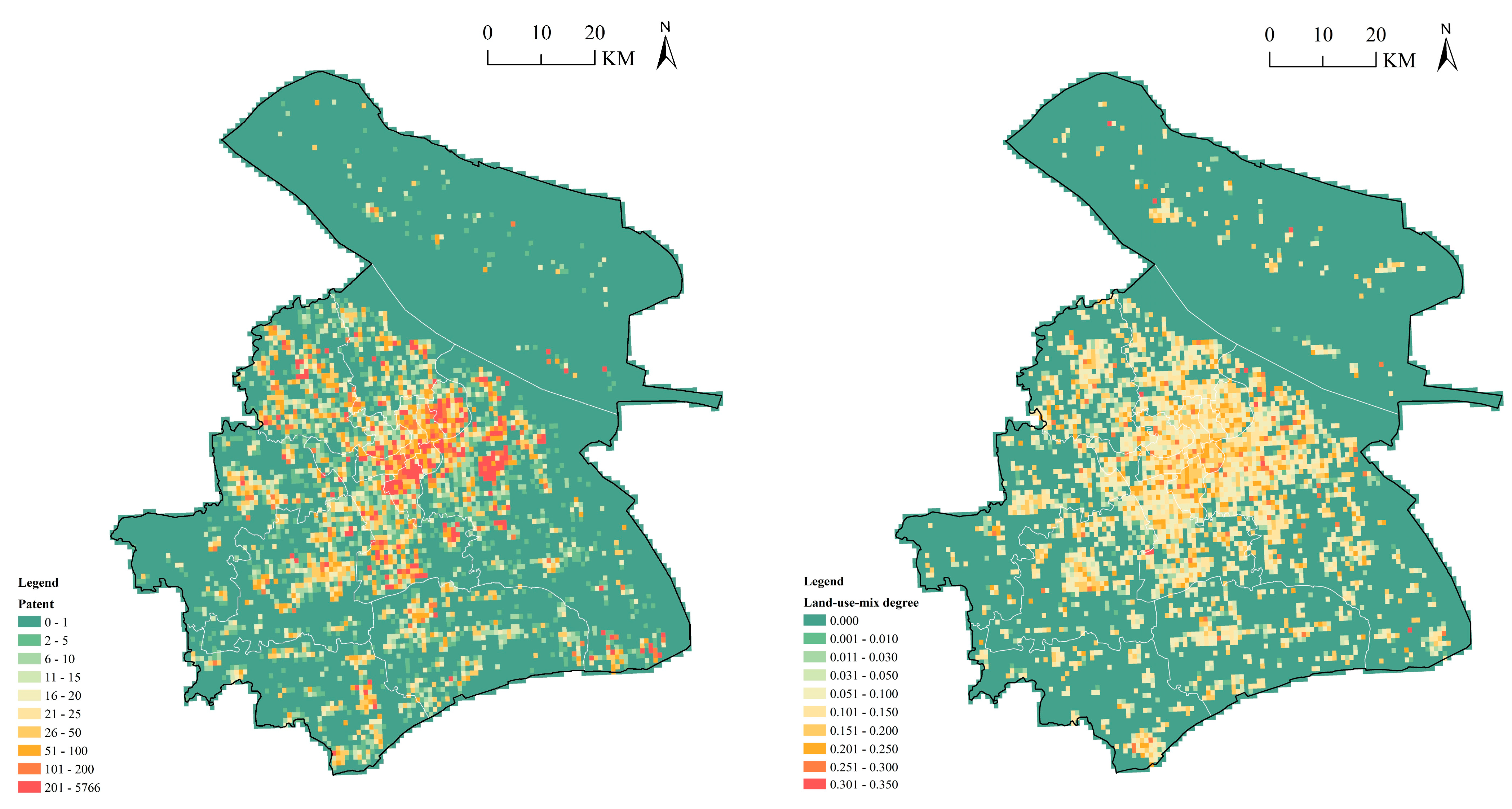
3.1. The Spatial Distribution of Technological Innovation and Land-Use Mix

Figure 2 depicts the spatial distribution of the number of patents and the degree of land-use mix at the grid cell level. With respect to the distribution of patents, we can obviously see that most of the grids have less than 25 patents. This can also be implied from Table 1 which shows that the mean value of the number of patents among grids is only 18.37, though the maximum value reaches 5766. Nonetheless, the distribution is characterized by a certain level of spatial autocorrelation. Specifically, grids with a larger number of patents tend to agglomerate in the urban core areas of Shanghai such as the Huangpu district, Jing’An district, and Hongkou district. In addition, we can observe the existence of some subcenters of technological innovation outside the urban core areas, such as those in the Pudong district, Fengxian district, and Jinsan district.

In terms of the spatial distribution of the degree of land-use mix, we can see that the distribution is to some extent similar to that of the number of patents. For instance, grids with a relatively higher level of land-use mix mainly agglomerate in the urban core areas of Shanghai, while some areas outside the urban core areas also contain grids with a higher degree of land-use mix. However, the differences in the degree of land-use mix among grids in urban core areas are not as significant as those revealed in the distribution of patents. The degree of land-use mix of most grids in urban core areas ranges from 0.1 to 0.2, suggesting that the overall level of land-use mix is relatively lower in Shanghai. This can also be reflected by Table 1 which shows that the mean and maximum values of the degree of land-use mix are only 0.03 and 0.34, respectively.

Furthermore, comparing the spatial distribution of the number of patents and the degree of land-use mix, we can find that the two variables are spatially correlated to some extent, indicating that technological innovation could be associated with land-use mix at the grid cell level. In the next subsection, the impact of land-use mix on technological innovation is empirically investigated.

3.2. The Estimation Results of Regression Models

Table 3. The regression results at the 1 km grid cell level.

Variables	(1)	(2)	(3)	(4)	(5)
$Mix$	1.099 ***		0.394 ***	0.305 ***	0.696 ***
	(0.046)		(0.039)	(0.038)	(0.088)
$Popu\_den$		1.010 ***	0.973 ***	0.618 ***	0.939 ***
		(0.782)	(0.077)	(0.071)	(0.078)
$Research\_den$		0.321 ***	0.248 ***	0.246 ***	0.211 ***
		(0.059)	(0.055)	(0.054)	(0.056)
$Metro\_dis$		−0.874 ***	−0.806 ***	−0.728 ***	−0.804 ***
		(0.035)	(0.036)	(0.035)	(0.036)
$Bus\_station$		0.901 ***	0.793 ***	0.707 ***	0.772 ***
		(0.053)	(0.052)	(0.050)	(0.052)
$Living\_facility$		−0.079	−0.098	0.071	−0.093
		(0.072)	(0.066)	(0.069)	(0.067)
$Hotel\_facility$		−0.095	−0.115 **	−0.170 ***	−0.102 *
		(0.061)	(0.055)	(0.054)	(0.056)
$Sport\_facility$		−0.189 **	−0.284 ***	−0.410 ***	−0.283 ***
		(0.080)	(0.075)	(0.071)	(0.075)
$W\ast Patent$				1.213 ***
				(0.095)
$Mix$∗$Mix$					−0.289 ***
					(0.073)
Constant	2.341 ***	1.632 ***	1.574 ***	1.423 ***	1.567 ***
	(0.035)	(0.000)	(0.031)	(0.030)	(0.031)
lnalpha	2.605 ***	2.357 ***	2.332 ***	2.263 ***	2.329 ***
	(0.019)	(0.020)	(0.020)	(0.020)	(0.020)
N	11,408	11,408	11,408	11,408	11,408
Pseudo R2	0.020	0.049	0.052	0.060	0.053

Note: (1) Standard errors are in parentheses; (2) *** p < 0.01; ** p < 0.05; * p < 0.1.

shows the estimation results of different negative binomial regression models which are run at the 1 km grid cell level. Note that the five regression models differ with each other mainly in terms of the variables that were considered. Nonetheless, the LR test indicator of lnalpha in all five regression models is statistically significant at the 1% level, indicating that all the regression models suffer from the over-dispersion issue, and therefore, the negative binomial regression model is more suitable than the Poisson regression model. Since the VIF value cannot be calculated after the negative binomial regressions, we re-run the regression models with the OLS method and calculate the VIF values of each variable. The results show that the variable of $Living\_facility$ has the largest VIF value of 6.24, and the mean VIF values of all the variables is less than 3. This suggests that the multicollinearity is not a serious issue. In addition, the independent variables in all five regression models were standardized, so their coefficients (i.e., their roles in facilitating the technological innovation process) are comparable. The estimation results of each regression model are discussed as follows.

In model (1), we only include the key independent variable $Mix$ in the regression model. Obviously, we can see that $Mix$ is statistically positive at the 1% significance level, suggesting that grids with a higher level of land-use mix tend to have more patents. This finding is generally in line with our theoretical expectation that land-use mix is likely to be positively associated with technological innovation. This result also resonates with the findings of existing studies that have investigated the impact of the built environment on technological innovation at the urban or regional level [14,15,16,19,20]. Though these studies have not specifically focused on the role of land-use mix on technological innovation, some studies have found that mixed land use could facilitate the technological innovation process [19,20]. As discussed above, mixed land use is conducive to diversity, walkability, and accessibility, which are all regarded as important factors accounting for technological innovation in the literature [22,26,29,32].

In model (2), we only investigate the impact of the seven control variables without including the key independent variable. The coefficients of the variables of $Popu\_den$, $Research\_den$, $Metro\_dis$, and $Bus\_station$ are statistically significant at the 1% level, and their signs are all as expected. This result suggests that both spatial agglomeration and accessibility are conducive to technological innovation. For instance, this result indicates that grids that are closer to metro stations are likely to be associated with more patents, ceteris paribus. Generally, this result is in line with the empirical findings of other studies that have analyzed the role of spatial agglomeration and accessibility in facilitating the technological innovation process [1,6,9,10,11,26,32]. However, the coefficients of the other three control variables, which reflect the impact of service facilities on technological innovation, are statistically insignificant (except for $Sport\_facility$), and their signs are all negative. This might be because the three control variables are highly correlated. In addition, the negative signs might indicate that grids with more service facilities tend to have higher housing or land prices, which could decrease their attractiveness for talented people and high-tech enterprises, especially those that are sensitive to housing and land prices. Therefore, too many service facilities could make a certain grid become less innovative due to the crowding-out effect of knowledge workers and high-tech enterprises. Note, however, that the above explanations are still hypothetical and lack empirical evidence, and detailed explanations for this result need further exploration but are beyond the scope of this paper.

In model (3), we include both the key independent variable and the seven control variables. Compared with the results of models (1) and (2), we can see that the coefficient of the key independent variable $Mix$ remains statistically significant, and its sign remains positive, suggesting that mixed land use is still positively associated with more patents after controlling for the impact of other variables. In addition, the coefficients of all the control variables (except for $Hotel\_facility$) remain unchanged in terms of their statistical significance and signs, suggesting that the impact of control variables is also stable. Since the coefficients are comparable, we can see that the role of land-use mix in facilitating the technological innovation process is relatively weaker than that of other control variables such as $Popu\_den$, $Metro\_dis$, and $Bus\_station$. Nonetheless, we argue that the role of land-use mix cannot be ignored since its coefficient is nearly half of that of $Popu\_den$, which is a traditional key contributor to technological innovation.

In model (4), we further include the spatially lagged dependent variable $W\ast Patent$ into model (3) to investigate whether spatial dependence exists in the impact of land-use mix on technological innovation. The coefficient of $W\ast Patent$ is statistically positive at the 1% significance level, indicating that the technological innovation capacity of a certain grid is likely to be positively associated with its neighboring grids. Furthermore, the coefficients and signs of the key independent variable and other control variables remain unchanged, implying that the result is stable after controlling for the impact of the spatially lagged dependent variable. Overall, this result is generally in line with the findings of other studies that have investigated the intra-urban geography of innovation [19,20]. In addition, such spatial dependence at a fine-grained geographical scale suggests that the impact of land-use mix on technological innovation could generate knowledge spillovers due to geographical proximity.

In model (5), we investigate whether the impact of land-use mix on technological innovation is linear or not by including the quadratic term of the key independent variable ($Mix$∗$Mix$) in model (3). As we can see, the coefficient of the quadratic term is statistically negative at the 1% significance level, while the coefficients and signs of the key independent variable and control variables remain unchanged in comparison with those in model (3). The result suggests that, other things being equal, grids with a too much higher level of land-use mix tend to have less patents. In other words, this finding implies an inverted U-curve relationship between land-use mix and technological innovation, which generally resonates with the findings of some studies that have shown an inverted U-curve relationship between third places and technological innovation at the grid cell level [20]. By investigating the land-use types of grids with the highest level of land-use mix, we find that most grids contain residential, commercial, public, and green space land, with relatively little space left for the development of high-tech enterprises. Therefore, we think this might be one of the possible reasons that account for an inverted U-curve relationship between land-use mix and technological innovation.

3.3. The Robustness Check

In this subsection, we check the robustness of the empirical results of different regression models by re-dividing the research area into 2 km × 2 km grid cells and by calculating the mixing degree of land use in other ways. The measurement of all the independent variables is the same as that based on the 1 km × 1 km grid cells.

First of all, we re-run the five regression models with the new division of grid cells while keeping the measurement of all the variables unchanged. As shown in

Table 4. Robustness check of the regression results at the 2 km grid cell level.

Variables	(1)	(2)	(3)	(4)	(5)
$Mix$	1.343 ***		0.485 ***	0.444 ***	0.771 ***
	(0.062)		(0.054)	(0.053)	(0.162)
$Popu\_den$		0.936 ***	0.986 ***	0.668 ***	0.958 ***
		(0.119)	(0.124)	(0.125)	(0.124)
$Research\_den$		0.529 ***	0.522 ***	0.312 ***	0.492 ***
		(0.095)	(0.094)	(0.089)	(0.095)
$Metro\_dis$		−0.871 ***	−0.723 ***	−0.689 ***	−0.726 ***
		(0.050)	(0.054)	(0.053)	(0.054)
$Bus\_station$		1.334 ***	1.159 ***	1.040 ***	1.109 ***
		(0.099)	(0.099)	(0.096)	(0.102)
$Living\_facility$		−0.275 *	−0.236	0.074	−0.240
		(0.162)	(0.157)	(0.166)	(0.158)
$Hotel\_facility$		−0.209 **	−0.213 **	−0.159 **	−0.192 **
		(0.093)	(0.088)	(0.078)	(0.090)
$Sport\_facility$		−0.635 ***	−0.733 ***	−0.989 ***	−0.710 ***
		(0.165)	(0.161)	(0.173)	(0.162)
$W\ast Patent$				0.782 ***
				(0.117)
$Mix$∗$Mix$					−0.265 *
					(0.139)
Constant	3.457 ***	2.880 ***	2.783 ***	2.717 ***	2.779 ***
	(0.051)	(0.046)	(0.045)	(0.045)	(0.045)
lnalpha	2.040 ***	1.816 ***	1.771 ***	1.738 ***	1.769 ***
	(0.030)	(0.031)	(0.032)	(0.032)	(0.032)
N	2946	2946	2946	2946	2946
Pseudo R2	0.028	0.053	0.058	0.062	0.058

Note: (1) Standard errors are in parentheses; (2) *** p < 0.01; ** p < 0.05; * p < 0.1.

, the significance and signs of the coefficients of the key independent variable and the control variables remain unchanged, compared with those in Table 3. This suggest that the basic empirical results of this paper are robust under different circumstances of grid division. Second, the spatially lagged dependent variable is statistically significant at the 2 km × 2 km grid cell level, suggesting that spatial spillovers of the impact of land-use mix on technological innovation still exist at a larger geographical scale. However, the coefficient of $W\ast Patent$ in Table 4 is smaller than that in Table 3, indicating that the spatial spillovers at the 2 km × 2 km grid cell level are relatively weaker than those measured at the 1 km × 1 km grid cell level. Furthermore, the quadratic terms of the key independent variable also remain negative and statistically significant, suggesting that the inverted U-curve relationship between land-use mix and technological innovation still holds. In summary, it can be argued that the impact of land-use mix on technological innovation is generally robust when dividing the research area in different ways.

Furthermore, we adopt two other approaches to measuring the mixing degree of land use. One is the Simpson approach, and the other is the Herfindahl–Hirschman index (HHI), which are described as follows. ${Simp\_Mix}_i$ and ${HHI\_Mix}_i$ represent the mixing degree of land use based on the Simpson approach and the HHI approach, respectively. $P_{ij}$ is the percentage of each land-use type $j$ in grid $i$.

$${Simp\_Mix}_i=1-{\sum }_{j=1}^k{P}_{ij}^2$$

(3)

$${HHI\_Mix}_i={\sum }_{j=1}^k{P}_{ij}^2$$

(4)

We replace the original key independent variable with the two other measures of land-use mix and re-run the regression model based on different units of analysis. As shown in

Table 5. Robustness check of the regression results using other two measures of land-use mix.

Variables	1 km × 1 km		2 km × 2 km
	Simpson Mix	HHI Mix	Simpson Mix	HHI Mix
$Mix$	0.718 ***	1.428 ***	0.863 ***	1.046 ***
	(0.038)	(0.042)	(0.057)	(0.074)
$Popu\_den$	0.658 ***	0.703 ***	0.866 ***	0.740 ***
	(0.073)	(0.060)	(0.123)	(0.106)
$Research\_den$	0.281 ***	0.169 ***	0.447 ***	0.487 ***
	(0.058)	(0.052)	(0.094)	(0.091)
$Metro\_dis$	−0.616 ***	−0.737 ***	−0.575 ***	−0.967 ***
	(0.036)	(0.037)	(0.053)	(0.050)
$Bus\_station$	0.662 ***	0.767 ***	0.953 ***	1.285 ***
	(0.049)	(0.048)	(0.091)	(0.094)
$Living\_facility$	−0.025	0.202 ***	−0.117	−0.144
	(0.064)	(0.067)	(0.157)	(0.165)
$Hotel\_facility$	−0.171 ***	−0.030	−0.294 ***	−0.191 *
	(0.045)	(0.059)	(0.089)	(0.109)
$Sport\_facility$	−0.321 ***	−0.372 ***	−0.616 ***	−0.631 ***
	(0.072)	(0.063)	(0.166)	(0.164)
$W\ast Patent$	0.566 ***	0.376 ***	0.221 ***	0.170 ***
	(0.059)	(0.037)	(0.064)	(0.050)
Constant	1.386 ***	1.004 ***	2.620 ***	2.616 ***
	(0.030)	(0.031)	(0.044)	(0.046)
lnalpha	2.247 ***	2.126 ***	1.690 ***	1.722 ***
	(0.020)	(0.020)	(0.032)	(0.031)
N	11,408	11,408	2946	2946
Pseudo R2	0.062	0.058	0.061	0.060

Note: (1) Standard errors are in parentheses; (2) *** p < 0.01; ** p < 0.05; * p < 0.1.

, the coefficients of the key independent variable represented by the two other measures remain positive and statistically significant, and the significance and signs of other control variables also remain unchanged. This suggests that our empirical results are also robust when measuring the mixing degree of land use in other ways.

4. Discussion and Policy Implications

4.1. Discussion

Nowadays, land-use mix has become an increasingly popular concept among scholars, urban planners, and policymakers. However, the extent to which land-use mix could facilitate the technological innovation process remains largely unexplored and lacks empirical evidence. In this sense, the empirical results of this paper make theoretical contributions to our understanding of the impact of land-use mix on technological innovation.

Specifically, the empirical results of this paper contribute to two different lines of literature. On the one hand, the literature on the geography of innovation has mainly focused on the influencing factors at the macrolevel [2,3,5,7], with relatively little attention being paid to investigating factors at a fine-grained geographical scale. Therefore, this paper contributes to this line of literature by examining micro-level factors that could affect the intra-urban geography of technological innovation at the 1 km * 1 km grid cell level. In doing so, we also aim to extend the traditional knowledge production function from the urban and regional levels to the intra-urban level. On the other hand, recent studies have paid increasing attention to the socioeconomic outcomes of the built environment such as people’s health [47] and the heat island effect [48]. Though some studies have also empirically investigated the relationship between the built environment and technological innovation [18,19,20], the question of how built environment factors could affect the spatial distribution of technological innovation at the intra-urban level remains to be empirically explored. In this sense, this paper contributes to this line of literature by analyzing the relationship between the built environment and technological innovation. Specifically, through the analysis of how land-use mix could facilitate the technological innovation process at the intra-urban level, this paper actively responds to the recent call for more attention to be paid to focusing on the socioeconomic effects of the built environment from the innovation perspective [20].

Our empirical results also resonate with some theoretical explanations of the complex innovation-making process. For instance, according to the 3D creativity management theory, which was proposed by Vuong and Napier [49] and further developed by Vuong et al. [50] and Nguyen et al. [51], the novelty and usefulness of a person’s creative ideas can be updated when these ideas are exchanged with others. Here, the exchange of ideas with others functions as filters that helps filter, refine, and re-evaluate the creativity of ideas, thus facilitating the complex process of technological innovation. In this sense, we think that the positive impact of mixed land use on technological innovation could relate to the filtering mechanisms through which the exchange of creative ideas is facilitated by mixed land use. In areas with a higher mixing degree of land use, people are more likely to come into contact with others engaging in various activities, due to the proximity of diverse facilities and shared spaces provided by land-use mix.

Though this paper contributes to a better understanding of the benefits of land-use mix from the perspective of technological innovation, it has some limitations that need to be further explored. First, since the same land-use mix index will correspond to multiple combinations of land-use types, it is essential to make more in-depth investigations to compare the impacts of multiple combinations of land-use types. Second, since not all technological innovation activities can lead to patents, empirical evidence based on other types of innovation data are thus needed to further examine the relationship between land-use mix and technological innovation. Third, future studies could utilize panel data and conduct more robustness checks, which could help demonstrate whether the relationship between land-use mix and technological innovation is causal and robust. Given that patents used in this study were applied for during the 2018–2020 period, a longitudinal analysis could also help mitigate the potential impact of COVID-19 on our empirical results.

4.2. Policy Implications

The empirical results of this paper also have some policy implications. First and foremost, we provided empirical evidence for the significant impact of mixed land use on facilitating the technological innovation process, which implies that local governments should emphasize the importance of land-use mix when aiming to promote innovation-driven development. In the Chinese context, however, land-use mix has been weakly associated with technological innovation in government policies, though promoting mixed land use has been emphasized in some big cities such as Shanghai. For instance, Chinese local governments have often considered land-use mix as being conducive to improving the efficiency of land use and promoting the sharing of public service facilities. Therefore, we hope that the empirical results of this paper could help local governments better understand the multi-faceted benefits of land-use mix, which are not only reflected by improving land-use efficiency but also by facilitating the technological innovation process. Second, policies aiming to improve the level of land-use mix of certain areas should also consider the spatial spillovers that might exist in the impact of land-use mix on technological innovation. As indicated by our empirical results, the land-use mix of a given area could not only affect its own technological innovation process but also the innovation capacity of its neighboring areas. Therefore, policymakers are recommended to consider such spatial spillovers when making land-use mix policies to facilitate the technological innovation process. Third, though land-use mix has been found to account for technological innovation, our empirical results also indicated that the over-mix of land use in a certain area could hinder the technological innovation process. Therefore, we suggest that local governments should be aware of not over-mixing land-use types in a certain area, which might generate the crowding-out effects of talented people and high-tech enterprises due to a rise in land and housing prices. In fact, our empirical results suggested that an intermediate level of land-use mix could generate the most benefits for technological innovation.

5. Conclusions

In this paper, we empirically investigate the relationship between land-use mix and technological innovation, aiming to bridge the research gap between the literature on the geography of innovation and the literature on the socioeconomic effects of the built environment. Drawing upon a database on the areas of interest of Shanghai, this paper employs the entropy index to measure the degree of land-use mix at the 1 km grid cell level. Furthermore, this paper draws upon the database on geo-coded patents to reflect the capacity of technological innovation at the grid cell level. Specifically, this paper adopts the negative binomial regression models to estimate the impact of land-use mix on technological innovation.

Our empirical results showed that grids with a higher level of land-use mix tend to have more patents, indicating that land-use mix is likely to be positively associated with technological innovation, ceteris paribus. Moreover, our empirical results demonstrated an inverted U-curve relationship between land-use mix and technological innovation, which indicates that over-mixing land-use types in certain areas could be detrimental to the technological innovation process. In addition, this paper showed that the impact of land-use mix on technological innovation has spatial spillovers, meaning that the land-use mix of a certain area could also affect the technological innovation capacity of its neighboring areas. It is also worth mentioning that our empirical results are robust under different circumstances in which the research area is divided in different ways.

References

1. Barra, C.; Ruggiero, N. How do dimensions of institutional quality improve Italian regional innovation system efficiency? The knowledge production function using SFA. J. Evol. Econ. 2022, 32, 591–642. [Google Scholar] [CrossRef]
2. McGuirk, H.; Lenihan, H.; Hart, M. Measuring the impact of innovative human capital on small firms’ propensity to innovate. Res. Policy 2015, 44, 965–976. [Google Scholar] [CrossRef]
3. Rodríguez-Pose, A.; Crescenzi, R. Research and development, spillovers, innovation systems, and the genesis of regional growth in Europe. Reg. Stud. 2008, 42, 51–67. [Google Scholar] [CrossRef]
4. Audretsch, D.B.; Feldman, M.P. R&D spillovers and the geography of innovation and production. Am. Econ. Rev. 1996, 86, 630–640. [Google Scholar]
5. Maggioni, M.A.; Nosvelli, M.; Uberti, T.E. Space versus networks in the geography of innovation: A European analysis. Pap. Reg. Sci. 2007, 86, 471–493. [Google Scholar] [CrossRef]
6. Peiró-Palomino, J. The geography of social capital and innovation in the European Union. Pap. Reg. Sci. 2019, 98, 53–73. [Google Scholar] [CrossRef]
7. Song, Y.; Yue, Q.; Zhu, J.; Zhang, M. Air pollution, human capital, and urban innovation in China. Environ. Sci. Pollut. Res. 2023, 30, 38031–38051. [Google Scholar] [CrossRef] [PubMed]
8. Wixe, S. Neighbourhood related diversity, human capital and firm innovation. Pap. Reg. Sci. 2018, 97, 217–252. [Google Scholar] [CrossRef]
9. Doloreux, D.; Shearmur, R. Does location matter? STI and DUI innovation modes in different geographic settings. Technovation 2023, 119, 102609. [Google Scholar] [CrossRef]
10. Donges, A.; Meier, J.M.; Silva, R.C. The impact of institutions on innovation. Manag. Sci. 2023, 69, 1951–1974. [Google Scholar] [CrossRef]
11. Florida, R.; Adler, P.; Mellander, C. The city as innovation machine. Reg. Stud. 2017, 51, 86–96. [Google Scholar] [CrossRef]
12. Liang, L.; Alam, A.; Sorwar, G.; Yazdifar, H.; Eskandari, R. The combined network effect of sparse and interlocked connections in SMEs’ innovation. Technol. Forecast. Soc. Chang. 2021, 163, 120488. [Google Scholar] [CrossRef]
13. Miguelez, E.; Moreno, R. Relatedness, external linkages and regional innovation in Europe. Reg. Stud. 2018, 52, 688–701. [Google Scholar] [CrossRef]
14. Fang, L.; Rao, F. When industry diversity meets walkability: An analysis of innovation in Baltimore, United States, and Melbourne, Australia. J. Plan. Educ. Res. 2021, 0739456X211042069. [Google Scholar] [CrossRef]
15. Bereitschaft, B. Exploring perceptions of creativity and walkability in Omaha, NE. City Cult. Soc. 2019, 17, 8–19. [Google Scholar] [CrossRef]
16. Hamidi, S.; Zandiatashbar, A. Does urban form matter for innovation productivity? A national multi-level study of the association between neighbourhood innovation capacity and urban sprawl. Urban Stud. 2019, 56, 1576–1594. [Google Scholar] [CrossRef]
17. Hamidi, S.; Zandiatashbar, A.; Bonakdar, A. The relationship between regional compactness and regional innovation capacity (RIC): Empirical evidence from a national study. Technol. Forecast. Soc. Chang. 2019, 142, 394–402. [Google Scholar] [CrossRef]
18. Li, Y.; Du, R. Polycentric urban structure and innovation: Evidence from a panel of Chinese cities. Reg. Stud. 2022, 56, 113–127. [Google Scholar] [CrossRef]
19. Wu, K.; Wang, Y.; Zhang, H.O.; Liu, Y.; Ye, Y. Impact of the built environment on the spatial heterogeneity of regional innovation productivity: Evidence from the Pearl River Delta, China. Chin. Geogr. Sci. 2021, 31, 413–428. [Google Scholar] [CrossRef]
20. Li, J.; Li, Y.; Tu, M.; Liu, X. Third places as catalysts for technological innovation? Evidence from a grid cell level analysis of Nanjing, China. Int. J. Urban Sci. 2023, 28, 105–123. [Google Scholar] [CrossRef]
21. Zhuo, Y.; Jing, X.; Wang, X.; Li, G.; Xu, Z.; Chen, Y.; Wang, X. The Rise and Fall of Land Use Mix: Review and Prospects. Land 2022, 11, 2198. [Google Scholar] [CrossRef]
22. Song, Y.; Merlin, L.; Rodriguez, D. Comparing measures of urban land use mix. Comput. Environ. Urban Syst. 2013, 42, 1–13. [Google Scholar] [CrossRef]
23. Abdullahi, S.; Pradhan, B.; Mansor, S.; Shariff, A.R.M. GIS-based modeling for the spatial measurement and evaluation of mixed land use development for a compact city. GIScience Remote Sens. 2015, 52, 18–39. [Google Scholar] [CrossRef]
24. Pang, M.; Chen, C.; Ma, L. Bilevel mixed land use–transportation model based on urban road network balance. J. Urban Plan. Dev. 2021, 147, 04021048. [Google Scholar] [CrossRef]
25. Ewing, R.; Cervero, R. Travel and the built environment. J. Am. Plan. Assoc. 2010, 76, 265–294. [Google Scholar] [CrossRef]
26. Seong, E.Y.; Lee, N.H.; Choi, C.G. Relationship between land use mix and walking choice in high-density cities: A review of walking in Seoul, South Korea. Sustainability 2021, 13, 810. [Google Scholar] [CrossRef]
27. Almansoub, Y.; Zhong, M.; Raza, A.; Safdar, M.; Dahou, A.; Al-qaness, M.A. Exploring the Effects of Transportation Supply on Mixed Land-Use at the Parcel Level. Land 2022, 11, 797. [Google Scholar] [CrossRef]
28. Su, S.; Zhang, Q.; Pi, J.; Wan, C.; Weng, M. Public health in linkage to land use: Theoretical framework, empirical evidence, and critical implications for reconnecting health promotion to land use policy. Land Use Policy 2016, 57, 605–618. [Google Scholar] [CrossRef]
29. Kamelifar, M.J.; Ranjbarnia, B.; Masoumi, H. The determinants of walking behavior before and during COVID-19 in middle-east and north Africa: Evidence from Tabriz, Iran. Sustainability 2022, 14, 3923. [Google Scholar] [CrossRef]
30. O’Driscoll, C.; Crowley, F.; Doran, J.; McCarthy, N. Land-use mixing in Irish cities: Implications for sustainable development. Land Use Policy 2023, 128, 106615. [Google Scholar] [CrossRef]
31. Koster, H.R.; Rouwendal, J. The impact of mixed land use on residential property values. J. Reg. Sci. 2012, 52, 733–761. [Google Scholar] [CrossRef]
32. Wei, Y.D.; Xiao, W.; Wen, M.; Wei, R. Walkability, land use and physical activity. Sustainability 2016, 8, 65. [Google Scholar] [CrossRef]
33. Florida, R. The creative class and economic development. Econ. Dev. Q. 2014, 28, 196–205. [Google Scholar] [CrossRef]
34. Katz, B.; Wagner, J. The Rise of Innovation Districts: A New Geography of Innovation in America; Brookings: Washington, DC, USA, 2014. [Google Scholar]
35. Kim, M. Spatial Qualities of Innovation Districts: How Third Places Are Changing the Innovation Ecosystem of Kendall Square; Massachusetts Institute of Technology: Boston, MA, USA, 2013. [Google Scholar]
36. Storper, M.; Venables, A.J. Buzz: Face-to-face contact and the urban economy. J. Econ. Geogr. 2004, 4, 351–370. [Google Scholar] [CrossRef]
37. Leyden, K.M. Social capital and the built environment: The importance of walkable neighborhoods. Am. J. Public Health 2003, 93, 1546–1551. [Google Scholar] [CrossRef] [PubMed]
38. Zheng, H.; Zhuo, Y.; Xu, Z.; Wu, C.; Huang, J.; Fu, Q. Measuring and characterizing land use mix patterns of China’s megacities: A case study of Shanghai. Growth Chang. 2021, 52, 2509–2539. [Google Scholar] [CrossRef]
39. Grant, J. Mixed use in theory and practice: Canadian experience with implementing a planning principle. J. Am. Plan. Assoc. 2002, 68, 71–84. [Google Scholar] [CrossRef]
40. Yue, Y.; Zhuang, Y.; Yeh, A.G.; Xie, J.Y.; Ma, C.L.; Li, Q.Q. Measurements of POI-based mixed use and their relationships with neighbourhood vibrancy. Int. J. Geogr. Inf. Sci. 2017, 31, 658–675. [Google Scholar] [CrossRef]
41. Zheng, M.; Wang, H.; Shang, Y.; Zheng, X. Identification and prediction of mixed-use functional areas supported by POI data in Jinan City of China. Sci. Rep. 2023, 13, 2913. [Google Scholar] [CrossRef]
42. Hoekman, J.; Frenken, K.; Van Oort, F. The geography of collaborative knowledge production in Europe. Ann. Reg. Sci. 2009, 43, 721–738. [Google Scholar] [CrossRef]
43. Li, Y.; Rigby, D. Relatedness, complexity, and economic growth in Chinese cities. Int. Reg. Sci. Rev. 2023, 46, 3–37. [Google Scholar] [CrossRef]
44. Aryal, G.R.; Mann, J.; Loveridge, S.; Joshi, S. Drivers of differences in inventiveness across urban and rural regions. J. Urban Aff. 2021, 43, 640–657. [Google Scholar] [CrossRef]
45. Bhaduri, B.; Bright, E.; Coleman, P.; Dobson, J. LandScan. Geoinformatics 2002, 5, 34–37. [Google Scholar]
46. Li, Y. Towards concentration and decentralization: The evolution of urban spatial structure of Chinese cities, 2001–2016. Comput. Environ. Urban Syst. 2020, 80, 101425. [Google Scholar] [CrossRef]
47. Wang, C.; Sheng, Y.; Wang, J.; Wang, Y.; Wang, P.; Huang, L. Air pollution and human health: Investigating the moderating effect of the built environment. Remote Sens. 2022, 14, 3703. [Google Scholar] [CrossRef]
48. Lan, T.; Peng, J.; Liu, Y.; Zhao, Y.; Dong, J.; Jiang, S.; Corcoran, J. The future of China’s urban heat island effects: A machine learning based scenario analysis on climatic-socioeconomic policies. Urban Clim. 2023, 49, 101463. [Google Scholar] [CrossRef]
49. Vuong, Q.; Napier, N. Making creativity: The value of multiple filters in the innovation process. Int. J. Transit. Innov. Syst. 2014, 3, 294–327. [Google Scholar] [CrossRef]
50. Vuong, Q.H.; Le, T.T.; La, V.P.; Nguyen, H.T.T.; Ho, M.T.; Van Khuc, Q.; Nguyen, M.H. Covid-19 vaccines production and societal immunization under the serendipity-mindsponge-3D knowledge management theory and conceptual framework. Humanit. Soc. Sci. Commun. 2022, 9, 22. [Google Scholar] [CrossRef]
51. Nguyen, M.H.; Jin, R.; Hoang, G.; Nguyen, M.H.T.; Nguyen, P.L.; Le, T.T.; Vuong, Q.H. Examining contributors to Vietnamese high school students’ digital creativity under the serendipity-mindsponge-3D knowledge management framework. Think. Ski. Creat. 2023, 49, 101350. [Google Scholar] [CrossRef]
Figure 1. The research area.
Land 13 00462 g001
Figure 2. The spatial distribution of patents (left) and land-use mix (right) at the grid level.
Land 13 00462 g002