Article

Modeling Geospatial Distribution of Peat Layer Thickness Using Machine Learning and Aerial Laser Scanning Data

1
Latvian State Forest Research Institute ‘Silava’, Rigas Str. 111, LV-2169 Salaspils, Latvia
2
Michael Succow Foundation, Greifswald Mire Centre, Ellernholzstr. 1/3, D-17489 Greifswald, Germany
*
Author to whom correspondence should be addressed.
Land 2024, 13(4), 466; https://doi.org/10.3390/land13040466
Submission received: 5 February 2024 / Revised: 26 March 2024 / Accepted: 4 April 2024 / Published: 5 April 2024

Abstract

:
Organic horizons including peat deposits are important terrestrial carbon pools, and various chemical, biological, and water exchange processes take place within them. Accurate information on the spatial distribution of organic soils and their properties is important for decision-making and land management. In this study, we present a machine learning approach for mapping the distribution of organic soils and determining the thickness of the peat layer using more than 24,000 peat layer thickness measurements obtained from field data, airborne laser scanning (ALS) data and various indices obtained from therein, as well as other cartographic materials. Our objectives encompassed two primary aims. Firstly, we endeavored to develop updated cartographic materials depicting the spatial distribution of peat layers. Secondly, we aimed to predict the depth of peat layers, thereby enhancing our understanding of soil organic carbon content. Continentality, a wet area map, latitude, a depth to water map with catchment area of 10 ha, and a digital elevation model were the most important covariates for the machine learning model. As a result, we obtained a map with three peat layer thickness classes, an overall classification accuracy of 0.88, and a kappa value of 0.74. This research contributes to a better understanding of organic soil dynamics and facilitates improved assessments of soil organic carbon stocks.

1. Introduction

Peatlands cover approximately three percent of the Earth’s land surface and hold a significant amount of organic soil carbon and freshwater resources [1]. According to the Intergovernmental Panel on Climate Change (IPCC), organic soils are identified on the basis of various criteria, and they should be at least 10 cm thick. In a shallow organic horizon, there should be at least 12 percent or more organic carbon when mixed to a depth of 20 cm [2,3]. These unique ecosystems are susceptible to destabilization due to climate change and anthropogenic pressures such as drainage and land use change. In boreal regions, the organic deposits in wetlands, agricultural land, and forests play a crucial role in storing carbon and influencing ecosystem productivity, nutrient cycling, and fire behavior [4]. Peatlands globally act as carbon sinks, storing a substantial amount of carbon and contributing to soil, atmospheric, and terrestrial biomass carbon stocks. However, estimating soil properties, such as peat layer thickness, remains a challenge [5].
In most soil mapping studies, researchers have delved into soils at various scales, from small plots [6,7] to regional and even global scopes [8,9]. Most studies have predominantly focused on predicting soil characteristics at a local to regional level. When it comes to mapping soil properties or classes, there is a noticeable connection between the size of the study area and the grid spacing used. Larger study areas often employ coarser resolutions, while smaller study areas tend to stick to standard resolutions. Regarding soil depth, many studies focus on the topsoil, but some dive into mapping properties at multiple depths [9,10].
Mapping of peat layer thickness is essential for understanding and managing peatland ecosystems. Various methods, such as in situ measurements of peat layer thickness and remote sensing technologies, are used to measure peat layer depth and derive necessary information [11]. In situ measurements involve manual probing of peat with a chamber corer or drill stick. These methods provide highly accurate data, but are cost and labor-intensive. Alternatively, remote sensing techniques, including optical and synthetic aperture radar (SAR) satellite imagery, ALS-based terrain indices, and machine learning algorithms, offer efficient and scalable approaches for digital organic soil deposit mapping. Remote sensing enables the acquisition of high-resolution data over large areas, allowing for the identification of peatland boundaries, variations in vegetation cover, surface roughness, and moisture content—indicators closely linked to peat layer depth [12]. Combining remote sensing data with machine learning algorithms enhances peat layer depth estimation by capturing complex relationships between peat layer thickness and environmental variables such as elevation, vegetation indices, climate data, and soil characteristics. This integration enables reliable prediction of peat layer thickness across vast peatland areas, supporting land use planning, carbon stock assessments, and conservation efforts.
Digital mapping techniques can support the compilation of accurate peatland maps to identify and prioritize regions that face significant threats and are key in driving change. These maps are valuable tools for assessing the sensitivity of peatlands to future climate change and their potential feedback within climate models. Integrating the protection, restoration, and management of peatlands into national climate change mitigation policies aligns with the goals outlined in the Paris Agreement [13]. Peat layer thickness estimation methods consider various covariates, including organism activities, topographic conditions, spatial positions, land cover, and geological aspects. Topographic covariates encompass slope, aspect, curvature, flow accumulation, wetness index, stream power index, landform classification, vegetation index, and soil mapping. Additionally, peatland visual conditions, such as length and slope condition, land cover, vegetation, and groundwater surface, exhibit specific correlations with peat layer thickness. It is essential to develop methods that encompass areas of peat overlain by non-peat forming vegetation to capture both actively forming and relic peats [11].
In this study, we combined peat layer thickness data obtained from field measurements and various land surface characterizing indices obtained from ALS data, along with various environmental parameters and machine learning methods, to develop a peat layer thickness map for the territory of Latvia. Peatland formation is directly dependent on local climate and topography [14]. In the territory of Latvia, the climatic conditions are determined by both oceanic and continental air masses [15], and in the variables of the predictive model they were characterized by geographical longitude and latitude, as well as the distance to the sea, i.e., continentality and height above sea level. Local topography, on the other hand, was characterized by slope data and various indices characterizing the movement and accumulation of water in the landscape (wet area maps, depth-to-water maps, and topographic wetness index). In addition, historical map data on soil texture and wetland distribution was used to estimate soil infiltration capacity. The developed data layer predicted the thickness of the peat layer in the entire territory of the country with a horizontal resolution of 5 m in three different classes of peat layer thickness. The predicted peat layer thickness classes are no peat (0 cm), thin peat layer (up to 20 cm), and thick peat layer (more than 20 cm). To avoid an unbalanced data set due to the limited amount of field data, more detailed depth classes were not distinguished.

2. Materials and Methods
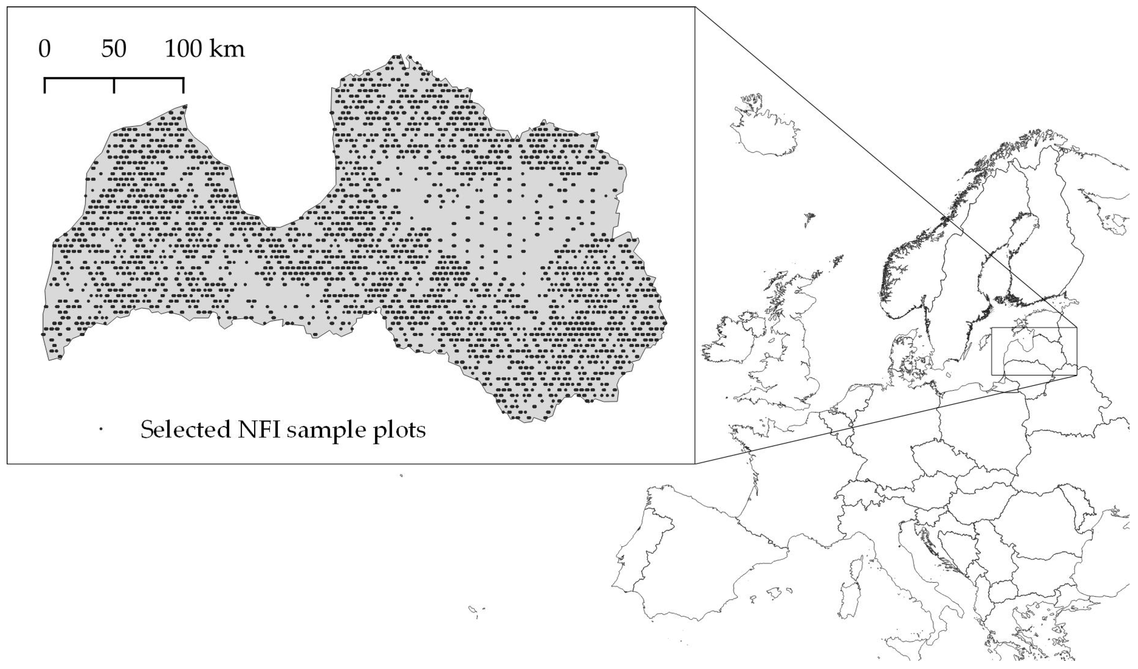
2.1. Study Site

The study area is located in Northern Europe between 55° and 59° N (WGS84) and 20° and 29° E. Mixed hemiboreal forests predominate in the area. The most common types of soil are glacial till, glacio-fluvial, lacustrine, aeolian, alluvial, organic, and other types of sediments [16]. According to historical soil maps, mire distribution data, forest growth condition data, peat extraction license data and other data sources, organic soils in Latvia cover 10.78% of land area. Data on organic soil coverage was derived from the results of a GIS supported paliduculture potential analysis in the frame of the EUKI Paludiculture project in the Baltics [17].

2.2. Field Data

In Latvia, the National Forest Inventory (NFI) was started in 2004, and there are more than 16,000 permanent sample plots covering the entire territory of the country. In the sample plots situated within forest land, in the period from 2014 to 2018, the thickness of the peat layer was determined with four repetitions on all sides, north, south, east, and west, 20 m away from the plot center (24,129 measurements). The depth of the peat layer was determined by using a soil probe and measuring the distance from the top layer of the soil to the boundary of the underlying mineral soil. The soil probe had a length of 70 cm. There are no IPCC definitions for peat and peatland, but the IPCC 2013 Wetlands Supplement follows the definition of organic soils in the 2006 IPCC Guidelines, where different limit depths of the organic horizon (10 and 20 cm) were found for different concentrations of organic carbon in the soil [18]. For the purpose of training the machine learning algorithm, the training data were grouped by different peat layer thickness classes (soils without an organic horizon, soils with a peat layer thickness of up to 20 cm, and soils where the thickness of the peat layer exceeds 20 cm).
The coordinates of the NFI plot centers were determined with an accuracy of less than 1 m. Since the data analysis used only those sample plots that represent forest land, the prediction of the spatial distribution of the peat layer thickness may be less accurate in inhabited areas and on agricultural land. The spatial distribution of the NFI plots used in the training of the machine learning models is shown in Figure 1.

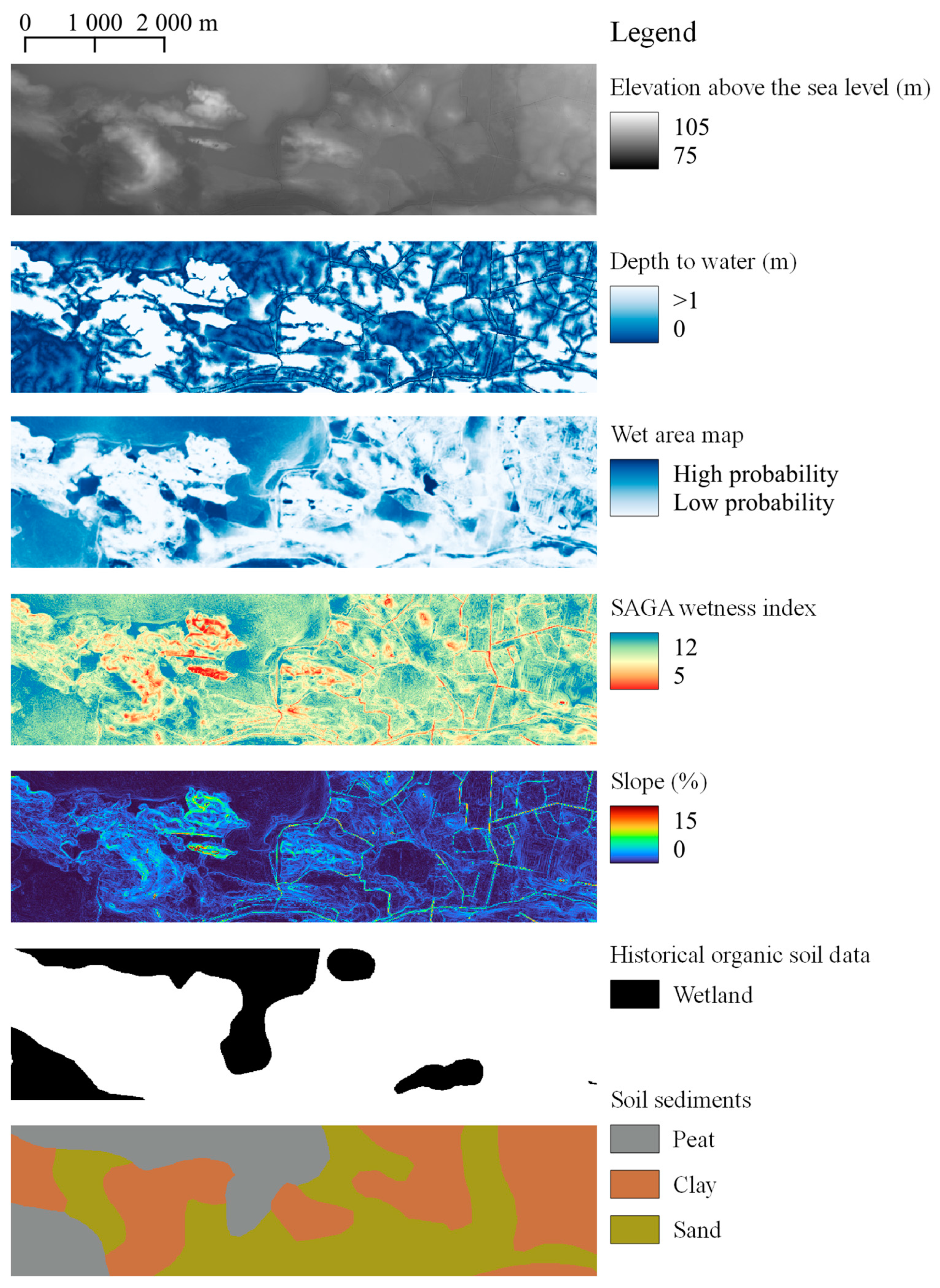
2.3. Variables Derived from ALS Data and Other Cartographic Materials

In order to predict the depth class of the peat layers, we used various indices obtained from the digital elevation model (DEM) and other cartographic materials. The DEM used to obtain the indices had a horizontal resolution of 5 m and was made from ALS data with a ground point density of at least 1.5 points per square meter, with vertical and horizontal errors of 12 and 36 cm, respectively. To improve data processing times, the DEM layer was divided into 50 × 50 km map sheets with a 1 km buffer. Data processing was carried out for the individual map sheets, and various indices characterizing the Earth’s surface were obtained, such as depth to water (DTW), wet area maps (WAM), surface slope, and SAGA wetness index. The individual map sheets were combined into a single layer after data processing to perform value extraction for the field data. Examples of the cartographic materials used for training the machine learning algorithm are shown in Figure 2 and described below.
  • Digital elevation model (DEM)
DEM with a horizontal resolution of 5 m was created from ALS data obtained from the Geospatial Information Agency of Latvia. The minimum ground point density is 1.5, and the vertical error of the input data is up to 12 cm, while the horizontal error is up to 36 cm.
  • Depth to water (DTW_10 and DTW_30)
DTW maps were based on the methodology described in [19]. DTW calculates the elevation along the least cost path starting from a known water body, providing insights into the predicted water table level. For the purposes of this research, the generation of water streams was carried out at two different catchment basin sizes: 10 and 30 ha. The cost surface for DTW prediction was calculated based on the DEM and the location of streams and other water bodies. DTW was calculated according to Equation (1).
D T W m = d z i d x i a x c ,
where dz/dx is the slope of a cell along the least-elevation path, i is a cell along the path, a equals one when the path crosses the cell parallel to cell boundaries and 2 when it crosses diagonally, and xc represents the grid cell size (m).
  • Wet area maps (WAM)
Wet area maps are designed as a prediction model with values between 0 and 1, where 0 and 1 indicate dry and wet soil conditions, respectively. An indicator for the presence of wet soil is a distinct layer of peat and/or a 50% proportion of reductimorphic colored soil. Wet area mapping methodology can be found in [20].
  • SAGA Wetness index (SAGA_TWI)
The SAGA Wetness Index employs an adapted approach to calculate catchment areas, leading to more precise estimations of soil moisture potential, particularly in valley regions close to water channels. This modification enhances the index’s ability to reflect realistic moisture conditions compared to the conventional topographic wetness index calculation method [21].
  • Slope
The slope of the surface was calculated using QGIS Raster terrain analysis tools. It calculated the slope from an input DEM layer. The slope is the angle of inclination of the terrain and is expressed in degrees.
  • Historical organic soil data (HOS)
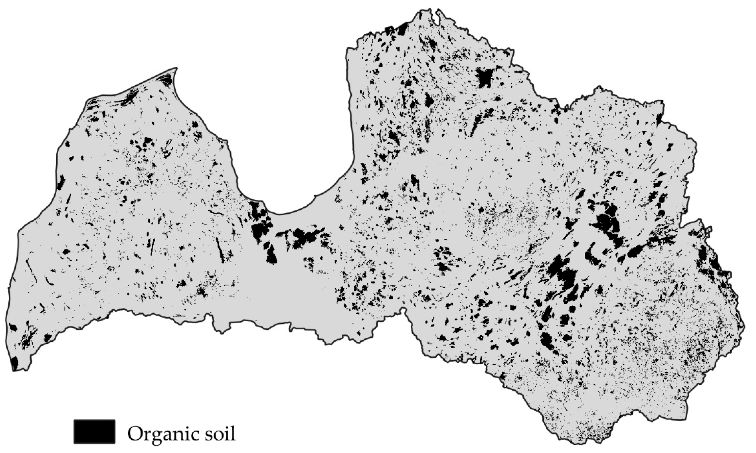
This data layer was created by combining historical soil maps, mire distribution data, forest growth condition data, peat extraction license data, and other data sources [17]. In the combined data set, it is possible to assess the distribution of historically mapped organic soils (Figure 3); however, information on the thickness of the peat layer is not available.
  • Soil data
Soil data refers to soil texture. A map of the distribution of sediments from the quaternary period [16] was used as the basis for the creation of the raster layer. The map shows the places where glacial till, glacio-fluvial, lacustrine, aeolian, alluvial, organic, and other sediments are found.
  • Proximity to water
Proximity to water is a raster layer that was created based on data on known water objects from the Latvian Geospatial Information Agency (LGIA). In the raster layer, each cell represents the distance in meters to the nearest lake, river, or stream. Distance to rivers and other bodies of water has previously been used in other similar studies to map peat layer thickness [22].
  • Continentality, X and Y coordinates
Finally, indicators such as continentality and geographical coordinates were calculated. The continentality in the raster layer indicated the distance of each cell to the Baltic Sea, while the geographic coordinate raster provided the opportunity to evaluate the influence of geographic latitude and longitude on changes in the thickness of the peat layer. High latitude is one aspect that provides the climatic conditions for peat formation in the boreal climate zone [23]. Our study area is located in hemiboreal conditions, so geographic location may have an impact on the spatial distribution of peatlands.

2.4. Machine Learning Classification of Peat Layer Thickness
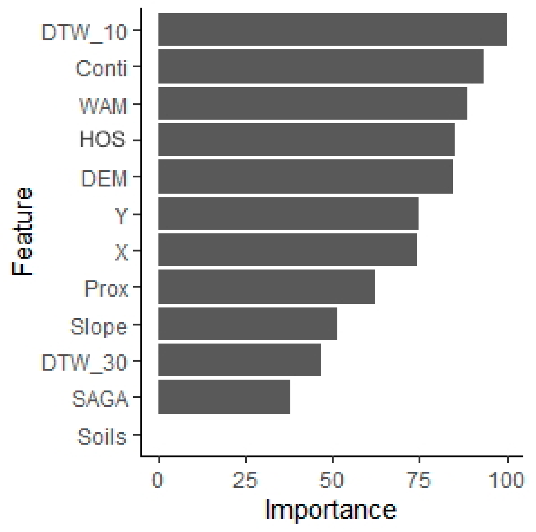
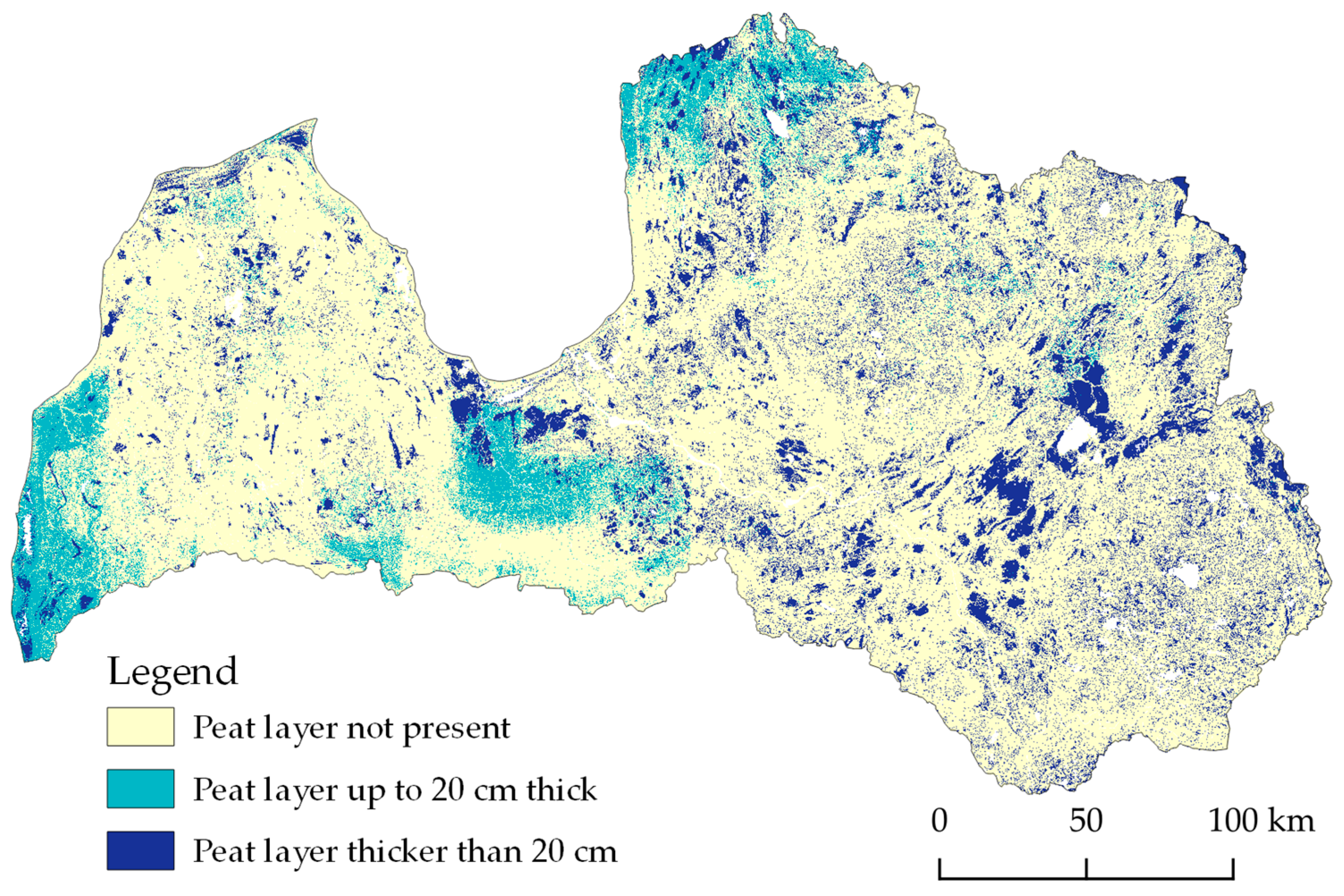
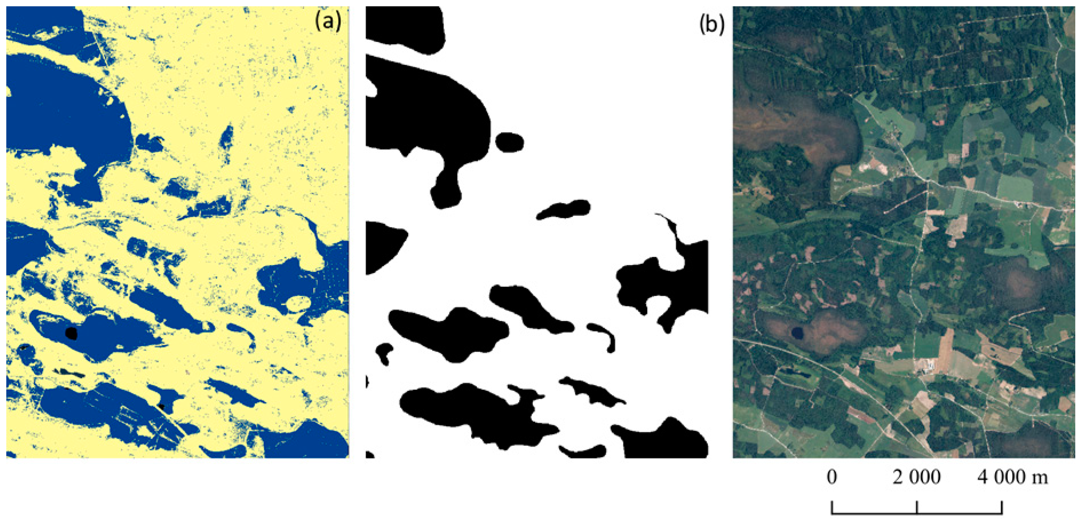
The classification of the thickness of the peat layers was performed using the R package “Caret” [24]. An NFI dataset with three peat layer thickness classes were split, randomly, into 80% training data and 20% test data. Several machine learning classification algorithms, such as xgbDART, xgbTREE, lda, and others were tested. Xgb algorithms construct an ensemble of decision trees. These decision trees are built recursively, dividing the feature space into distinct regions, where each region corresponds to a prediction. Unlike conventional decision trees that tend to grow deep structures, XGBoost prefers to use shallow trees, often referred to as “weak” learners [25]. In order to eliminate the effects caused by an imbalanced dataset, several algorithms were tested, including an over-sampling, under-sampling [26], and SMOTE [27] algorithm. All models were parameterized and tuned using a grid-search approach in combination with four-fold cross-validation to find the best-fitting model. Four-fold cross-validation serves as a prevalent method for assessing machine learning model performance. It involves splitting the dataset into four equal-sized subsets, termed folds. Three folds are utilized for model training, while the remaining fold serves as the validation set. This cycle is reiterated four times, ensuring each fold acts as the validation set once. Finally, the average performance metrics across iterations yields a reliable estimation of the model’s effectiveness [28]. The tuned models were applied on the test dataset and evaluated using Cohen’s kappa index of agreement.

3. Results

The highest classification accuracy and kappa value was observed in the machine learning model based on the xgbTREE algorithm using the over-sampling method. The xgbTREE method, a part of the XGBoost algorithm, employs decision trees as base learners in a boosting framework, effectively capturing complex data patterns and yielding accurate predictions through iterative refinement. The importance of various remote sensing data and cartographic materials on the classification results is shown in Figure 4. This helps to determine the significance of each feature in influencing the decision-making procedure of the model. A higher score assigned to a feature indicates a more substantial impact on the model’s ability to predict a specific variable. The most important machine learning parameters in this case were the depth to water map with a catchment size of 10 ha, continentality, wet area maps, and the historic organic soil map.
The accuracy of the overall machine learning classification algorithm reached 0.88, while the kappa value was 0.75. Separately, by different classes, sensitivity and specificity reached:
  • Soils without organic horizon—0.95 (sensitivity), 0.80 (specificity);
  • Soils with peat layer up to 20 cm—0.62 (sensitivity), 0.97 (specificity);
  • Soils with peat layer thicker than 20 cm—0.82 (sensitivity), 0.96 (specificity).
Table 1 displays the confusion matrix derived from the test dataset, elucidating the reasons behind the comparatively lower classification accuracy in the shallow peat class compared to other classes. Despite the relatively small number of false positives when considering the observations in other classes, false negative predictions accounted for 38.6% of cases. Notably, three-quarters of these false negatives were anticipated in a class where peat was entirely absent.
The classification results for the territory of Latvia can be seen in Figure 5. The results suggested that within Latvia, approximately 15.6% (9760 km2) of the total land area is covered by soils where peat layer thickness exceeds 20 cm, with an additional 7.6% (4799 km2) of the territory being covered by a peat layer with thickness less than 20 cm. These results indicate a difference from the previously known area of organic soils, which was 10.8%. This difference can be explained by the different accuracy of organic soil mappings and the area size to be resolved. During the assessment of the precision of current organic soil distribution maps in comparison to data obtained from National Forest Inventory (NFI) sample plots, the overall accuracy reached 0.76, with a corresponding kappa value of 0.39. Comparing these indicators, it can be concluded that the application of the used machine learning algorithm provided significant improvements in the understanding of the distribution of organic soils in Latvia.

4. Discussion

Efforts directed towards mapping the spatial distribution of peat using remote sensing data have conventionally leaned upon techniques such as aerial photography [29] or satellite imagery [30], depending on the survey area. However, organic soils often lie beneath vegetation types unrelated to peat formation conditions, and the presence of peat cannot be reliably inferred from the vegetation cover, especially near the edges of peatlands where human activities have disturbed natural processes between the vegetation and underlying peat. Contrary to classical approaches, our study relies entirely on remote sensing data that can penetrate vegetation and does not take into account the signal or interference from naturally growing and/or human-modified vegetation cover and degradation and loss of organic soil layers by drainage and land use.
This study has yielded a cartographic output delineating the spatial distribution of organic soils across the Latvian landscape, alongside providing insights into the thickness of the peat layer for each individual pixel on the map. By evaluating the depth of different soil layers and their properties, prediction models were developed to determine the exact depth of the soil layer [12] or to predict soil properties using layers of 10, 20, or 50 cm, or other slices [31,32]. Since the field data available to us measured the thickness of the peat layer in centimeters with a maximum depth of 70 cm, we divided it into 3 classes: 0 cm, 1–20 cm, and >20 cm. The maximum thickness of the peat layer for soils where it exceeded 70 cm is unknown to us.
In the maps available so far, organic soils have been mapped mostly in historical agricultural lands or extensive wetlands, while detailed soil mapping has not been carried out in historical forest lands. More than 24,000 peat layer depth measurement points were used in this study, and comparing these data with historical maps, it can be concluded that their accuracy reached only 0.75 and their kappa value 0.39. For the newly developed product, the overall value reached 0.88, and the kappa value reached 0.74. Using various indices that characterize elevation, obtained from ALS data, ref. [33] achieved an accuracy of 0.89–0.91 when mapping the spatial distribution of peatlands in the Swedish forest landscape in 10 m horizontal resolution. Using multispectral satellite imagery from the Landsat 8 mission, ref. [34] mapped the spatial distribution of organic soils in Scotland at 100 m horizontal resolution. When classifying the soil into three classes (mineral, organo-mineral, and organic) the total accuracy reached 69.8%, and when classifying the territory into two classes (non-organic and organic), the accuracy reached 86.4%.
Although the accuracy of the overall classification algorithm reached 0.88, for soils with a shallow layer of peat, its sensitivity reached only 0.62. Low sensitivity for a specific class in a machine learning model can be attributed to various factors, such as class imbalance, feature representation, data quality, model complexity, etc. [35,36]. To eliminate these problems, we processed the training data by balancing the data set using the upsampling method, artificially generating new data rows for classes that are less represented. An additional potential challenge could arise from the resemblance of various topographic parameters between soils lacking a peat layer and those featuring a shallow peat layer. This similarity can result in lower sensitivity for the shallow peat class, as the model may struggle to differentiate subtle differences between the presence of a shallow peat layer and the absence of a peat layer [37]. Indeed, three-quarters of the false negatives for shallow peat were classified as soil without a peat layer.
The cartographic data obtained in our study show that there are more organic soils in the territory of Latvia than thought before now. One of the reasons for this difference is the scale and size of the mapping unit, resulting in different levels of aggregation of presented information. With the improvement of remote sensing technologies and data processing methods, it is possible to model and map various environmental parameters much more precisely than in the 1960 and 1970s, when mapping was performed in an analog fashion. Various studies related to soil mapping have shown that studies have been conducted at all scales, from the field level (<1 km2) to the global scale (>107 km2). Likewise, the data resolution for these studies has varied from a few meters to several kilometers. Mostly, the resolution of the maps has been in the range of 30–250 m [38]. Such resolution may be related to the availability of remote sensing data. The data resolution used in our study is 5 m, which is common for data layers generated using ALS data.
The effect of mapping scale is found in any field that attempts to describe spatial objects, and the sensitivity and precision of classification of various environmental elements typically increases with the application of methods suitable for small scales. In contrast, larger scale maps are too generalized to correctly delineate the complex, irregular outlines of large areas, and too coarse to completely detect smaller scale objects [39]. Figure 6 shows a randomly selected region and depicts a map developed with machine learning methods, the historical spatial distribution of organic soils, and an orthophoto mosaic. It can be seen that the developed map correlates closely with what is seen in the historical data; however, the higher resolution gives a greater degree of detail. The geometries depicted in the historical map have now become more complex; in some places the geometries have protrusions, while in others the model indicates indentations, thereby correcting the contours of the geometries depicted in the historical maps. In addition, relatively large areas with a layer of peat appear in previously unmapped areas. Local small areas with the presence of a peat layer also appear on the new map, almost like noise.
Determining the exact depth of the peat layer at a small scale can be difficult due to the unknown and possibly complex topography of the underlying mineral deposits [40]. However, by identifying areas where the land surface relief indicates a long-term high soil moisture regime, it is possible to identify places where peat has accumulated for a long time and, therefore, in a thicker layer [41]. In the course of this study, we included several covariates characterizing soil moisture, such as WAM and DTW maps, while developing the machine learning model. As can be seen in Figure 3, these two covariates are relatively high in the scale of feature importance in the development of the machine learning model.
This study uses various land surface characterizing indices, which are basically obtained from laser scanning data, such as DEM, slope, WAM, DTW and SAGA TWI, and various cartographic materials such as a historical soil map, quaternary sediment map, etc., as well as geographical characteristics such as X and Y coordinates, continentality, and distance to rivers/lakes. Deragon et al. [42] showed that in cultivated agricultural lands, the concentration of various chemical elements on the surface of the soil (thorium, uranium), various topographic indices, such as multiresolution index of the ridge top flatness and valley bottom flatness, and mid-slope position, as well as distance from each peatland’s center and other covariates, can all be important in mapping organic soils using machine learning [12]. Gatis et al. demonstrated that passive airborne gamma-ray spectrometric data can also be used in peat layer thickness mapping. Total air absorbed dose rates of thorium, uranium, and potassium, referred to as radiometric dose, together with the slope data, can explain 72–73 percent of the peat layer thickness variability with RMSE of 0.27 m. However, such data are not available for the study area, so their importance cannot be compared.
The developed model in this study has shortcomings for modeling the distribution of deep organic soils and peatlands. Depending on the availability and detail of field data, it may be feasible to predict the depth of considerably deeper peat strata, such as those found in tropical peatlands, by using terrain data and various indices characterizing soil moisture [22]. In conventional forestry and agricultural management, organic soils are drained with summer water levels up to 1 m, and deeper below surface level, leading to high GHG emissions due to the decomposition of organic matter. Given that it only addresses three depth classes, with the deepest class stopping at >70 cm, the model is too vague for a priori evaluation of suitable land use change and CCM measures for drained organic soils. By stopping drainage and implementing rewetting, the GWP of such sites can be reduced despite increased methane emissions, which are potentially induced by rewetting measures [43]. The inclusion of additional international acknowledged classifications for peat and peatlands [44] would improve compatibility with other international maps and data collections [45]. Peatland rewetting and stabilized high water levels close to the surface can be combined with the implementation of wet agricultural or forestry management (paludiculture) [46].
Paludiculture can be a supportive option in regional spatial planning of climate change mitigation pathways in the land use sector [47]. Suitable plants for the Holarctic region for cultivation or use in paludicultures to provide biomass for materials, fodder, or renewable biomass fuels are described in, and partly known from, traditional utilization schemes [48]. Existing gaps in paludiculture value creation chains, and obstacles in framework policies and programs that hinder economic viability and upscaling of paludicultures, are and will be funded and monitored in long-term and large scale paludiculture demonstration sites in Germany [49] and wider Europe [50]. To identify potential implementation areas for paludiculture and to model and evaluate long-term effects on the climate under different land use options, knowledge on the depths and extents of organic and peat soils at implementation sites is essential. A differentiation of more classes and inclusion of further data sets assessing also total organic soil depths would improve the model developed in this study, making it fit for spatial a priori evaluation and decision-making in land use change for climate change mitigation.

5. Conclusions

In this study, we have developed a map of organic soil distribution and peat layer thickness for the territory of Latvia using peat layer thickness data from NFI sample plots, remote sensing data, various cartographic materials, and machine learning methods. The thickness of peat layers has been mapped in three classes (0 cm, <20 cm, and >20 cm), and the overall classification accuracy reached 88% (kappa value = 0.74). Using a machine learning approach, we identified important variables derived from ALS data and other cartographic materials that influenced the classification results, such as continentality, wet area maps, latitude, and depth to water maps. The results of our study provide an improved understanding of organic soil distribution and an improvement in the accuracy of related maps. The developed map shows that soils with a peat layer thickness exceeding 20 cm cover 15.6% of the study area, and soils with a thickness of less than 20 cm cover an additional 7.6%. These findings highlight the potential of using remote sensing data and machine learning techniques for accurate mapping of organic soils. The approach used in this study helps to improve the prediction of the distribution of organic soils. The developed map for Latvia can contribute to better land management, conservation efforts, and carbon stock assessments.
For spatial evaluation and decision-making, further improvements to the model are recommended, e.g., inclusion of further international peatland classifications, suitable datasets, and field assessments which address total depth of organic horizons and allow for a more differentiated soil layer classification. In combination with modeling of water availability and improvement options for catchment level, this will significantly help to improve the applicability of the model for the prioritization of sites and determination of suitable CCM measures.

Author Contributions

Conceptualization, J.I.; Data curation, J.I.; Formal analysis, J.I.; Methodology, J.I.; Visualization, J.I.; Writing—original draft, J.I. and A.H.; Writing—review and editing, J.I., A.H. and R.M. All authors have read and agreed to the published version of the manuscript.

Funding

This research was funded the project “Demonstration of climate change mitigation potential of nutrients rich organic soils in Baltic States and Finland” (LIFE OrgBalt, LIFE18 CCM/LV/001158).

Data Availability Statement

Data available on request made to the corresponding author, Janis Ivanovs. Final map available as WMS service at: https://silava.forestradar.com/geoserver/silava/wms.

Conflicts of Interest

The authors declare no conflicts of interest. The funders had no role in the design of the study; in the collection, analyses, or interpretation of data; in the writing of the manuscript; or in the decision to publish the results.

References

  1. Minasny, B.; Berglund, Ö.; Connolly, J.; Hedley, C.; de Vries, F.; Gimona, A.; Kempen, B.; Kidd, D.; Lilja, H.; Malone, B.; et al. Digital Mapping of Peatlands—A Critical Review. Earth-Sci. Rev. 2019, 196, 102870. [Google Scholar] [CrossRef]
  2. IPCC. 2013 Supplement to the 2006 IPCC Guidelines for National Greenhouse Gas Inventories: Wetlands; Hiraishi, T., Krug, T., Tanabe, K., Srivastava, N., Baasansuren, J., Fukuda, M., Troxler, T.G., Eds.; IPCC: Geneva, Switzerland, 2014; ISBN 978-92-9169-139-5. [Google Scholar]
  3. Couwenberg, J. Greenhouse Gas Emissions from Managed Peat Soils: Is the IPCC Reporting Guidance Realistic? Mires Peat 2011, 8, 2. [Google Scholar]
  4. Kurz, W.A.; Shaw, C.H.; Boisvenue, C.; Stinson, G.; Metsaranta, J.; Leckie, D.; Dyk, A.; Smyth, C.; Neilson, E.T. Carbon in Canada’s Boreal Forest-A Synthesis. Environ. Rev. 2013, 21, 260–292. [Google Scholar] [CrossRef]
  5. Beucher, A.; Koganti, T.; Iversen, B.V.; Greve, M.H. Mapping of Peat Thickness Using a Multi-Receiver Electromagnetic Induction Instrument. Remote Sens. 2020, 12, 2458. [Google Scholar] [CrossRef]
  6. Pouladi, N.; Møller, A.B.; Tabatabai, S.; Greve, M.H. Mapping Soil Organic Matter Contents at Field Level with Cubist, Random Forest and Kriging. Geoderma 2019, 342, 85–92. [Google Scholar] [CrossRef]
  7. Kalambukattu, J.G.; Kumar, S.; Arya Raj, R. Digital Soil Mapping in a Himalayan Watershed Using Remote Sensing and Terrain Parameters Employing Artificial Neural Network Model. Environ. Earth Sci. 2018, 77, 203. [Google Scholar] [CrossRef]
  8. Ramcharan, A.; Hengl, T.; Nauman, T.; Brungard, C.; Waltman, S.; Wills, S.; Thompson, J. Soil Property and Class Maps of the Conterminous United States at 100-Meter Spatial Resolution. Soil Sci. Soc. Am. J. 2018, 82, 186–201. [Google Scholar] [CrossRef]
  9. Hengl, T.; De Jesus, J.M.; Heuvelink, G.B.M.; Gonzalez, M.R.; Kilibarda, M.; Blagotić, A.; Shangguan, W.; Wright, M.N.; Geng, X.; Bauer-Marschallinger, B.; et al. SoilGrids250m: Global Gridded Soil Information Based on Machine Learning. PLoS ONE 2017, 12, e0169748. [Google Scholar] [CrossRef]
  10. Lacoste, M.; Minasny, B.; McBratney, A.; Michot, D.; Viaud, V.; Walter, C. High Resolution 3D Mapping of Soil Organic Carbon in a Heterogeneous Agricultural Landscape. Geoderma 2014, 213, 296–311. [Google Scholar] [CrossRef]
  11. Cahyono, B.K.; Aditya, T. Istarno The Least Square Adjustment for Estimating the Tropical Peat Depth Using LiDAR Data. Remote Sens. 2020, 12, 875. [Google Scholar] [CrossRef]
  12. Gatis, N.; Luscombe, D.J.; Carless, D.; Parry, L.E.; Fyfe, R.M.; Harrod, T.R.; Brazier, R.E.; Anderson, K. Mapping Upland Peat Depth Using Airborne Radiometric and Lidar Survey Data. Geoderma 2019, 335, 78–87. [Google Scholar] [CrossRef]
  13. Crooks, S.; Herr, D.; Tamelander, J.; Laffoley, D.; Vandever, J. Mitigating Climate Change through Restoration and Management of Coastal Wetlands and Near-Shore Marine Ecosystems: Challenges and Opportunities; World Bank: Washington, DC, USA, 2011. [Google Scholar]
  14. Anderson, R.L.; Foster, D.R.; Motzkin, G. Integrating Lateral Expansion into Models of Peatland Development in Temperate New England. J. Ecol. 2003, 91, 68–76. [Google Scholar] [CrossRef]
  15. Draveniece, A. Oceanic and Continental Air Masses over Latvia. Latvijas Veģetācija; Laivins, M., Ed.; SIA PIK: Riga, Latvia, 2007. [Google Scholar]
  16. Meirons, Z. Kvartāra Nogulumi. M.:1:200 000; Valsts Ģeoloģijas Dienests: Riga, Latvia, 2002. [Google Scholar]
  17. Piirimäe, K.; Salm, J.-O.; Ivanovs, J.; Stivrins, N.; Greimas, E.; Jarašius, L.; Zabeckis, N.; Haberl, A. Paludiculture in the Baltics-GIS Study, Project Assessment Report; Estonian Fund for Nature & Succow Foundation partner in the Greifswald Mire Centre, 2020; 48p, Available online: https://media.voog.com/0000/0037/1265/files/GIS_EE_LV_LT_04.2020.pdf (accessed on 2 February 2024).
  18. FAO. Peatland Mapping and Monitoring–Recommendations and Technical Overview; FAO: Rome, Italy, 2020. [Google Scholar]
  19. Murphy, P.N.C.; Ogilvie, J.; Castonguay, M.; Zhang, C.; Meng, F.-R.; Arp, P.A. Improving Forest Operations Planning through High-Resolution Flow-Channel and Wet-Areas Mapping. For. Chron. 2008, 84, 568–574. [Google Scholar] [CrossRef]
  20. Ivanovs, J.; Lupikis, A. Identification of Wet Areas in Forest Using Remote Sensing Data. Agron. Res. 2018, 16, 2049–2055. [Google Scholar] [CrossRef]
  21. Böhner, J.; Selige, T. Spatial Prediction of Soil Attributes Using Terrain Analysis and Climate Regionalisation. Gott. Geogr. Abh. 2006, 115, 13–28. [Google Scholar]
  22. Rudiyanto; Minasny, B.; Setiawan, B.I.; Arif, C.; Saptomo, S.K.; Chadirin, Y. Digital Mapping for Cost-Effective and Accurate Prediction of the Depth and Carbon Stocks in Indonesian Peatlands. Geoderma 2016, 272, 20–31. [Google Scholar] [CrossRef]
  23. Vasander, H.; Kettunen, A. Carbon in Boreal Peatlands. In Boreal Peatland Ecosystems; Kelman Wieder, R., Vitt, D.H., Eds.; Springer: Berlin/Heidelberg, Germany, 2006; Volume 188, pp. 165–194. ISBN 978-3-540-31912-2. [Google Scholar]
  24. Kuhn, M. Building Predictive Models in R Using the Caret Package. J. Stat. Softw. 2008, 28, 1–26. [Google Scholar] [CrossRef]
  25. Chen, T.; Guestrin, C. XGBoost: A Scalable Tree Boosting System. In Proceedings of the ACM SIGKDD International Conference on Knowledge Discovery and Data Mining, San Francisco, CA, USA, 13–17 August 2016; Association for Computing Machinery: New York, NY, USA, 2016; pp. 785–794. [Google Scholar]
  26. Cordón, I.; García, S.; Fernández, A.; Herrera, F. Imbalance: Oversampling Algorithms for Imbalanced Classification in R. Knowl.-Based Syst. 2018, 15, 329–341. [Google Scholar] [CrossRef]
  27. Chawla, N.V.; Bowyer, K.W.; Hall, L.O.; Kegelmeyer, W.P. SMOTE: Synthetic Minority over-Sampling Technique. J. Artif. Intell. Res. 2002, 16, 321–357. [Google Scholar] [CrossRef]
  28. Ramezan, C.A.; Warner, T.A.; Maxwell, A.E. Evaluation of Sampling and Cross-Validation Tuning Strategies for Regional-Scale Machine Learning Classification. Remote Sens. 2019, 11, 185. [Google Scholar] [CrossRef]
  29. Cruickshank, M.M.; Tomlinson, R.W. Peatland in Northern Ireland: Inventory and Prospect. Irish Geogr. 1990, 23, 17–30. [Google Scholar] [CrossRef]
  30. Fuller, R.M.; Smith, G.M.; Sanderson, J.M.; Hill, R.A.; Thomson, A.G. The UK Land Cover Map 2000: Construction of a Parcel-Based Vector Map from Satellite Images. Cartogr. J. 2002, 39, 15–25. [Google Scholar] [CrossRef]
  31. Mulder, V.L.; Lacoste, M.; Richer-de-Forges, A.C.; Martin, M.P.; Arrouays, D. National versus Global Modelling the 3D Distribution of Soil Organic Carbon in Mainland France. Geoderma 2016, 263, 16–34. [Google Scholar] [CrossRef]
  32. Adhikari, K.; Hartemink, A.E.; Minasny, B.; Bou Kheir, R.; Greve, M.B.; Greve, M.H. Digital Mapping of Soil Organic Carbon Contents and Stocks in Denmark. PLoS ONE 2014, 9, e105519. [Google Scholar] [CrossRef] [PubMed]
  33. Rimondini, L.; Gumbricht, T.; Ahlström, A.; Hugelius, G. Mapping of Peatlands in the Forested Landscape of Sweden Using LiDAR-Based Terrain Indices. Earth Syst. Sci. Data Discuss. 2023, 15, 3473–3482. [Google Scholar] [CrossRef]
  34. Aitkenhead, M.J. Mapping Peat in Scotland with Remote Sensing and Site Characteristics. Eur. J. Soil Sci. 2017, 68, 28–38. [Google Scholar] [CrossRef]
  35. Thabtah, F.; Hammoud, S.; Kamalov, F.; Gonsalves, A. Data Imbalance in Classification: Experimental Evaluation. Inf. Sci. 2020, 513, 429–441. [Google Scholar] [CrossRef]
  36. Naboureh, A.; Li, A.; Bian, J.; Lei, G.; Amani, M. A Hybrid Data Balancing Method for Classification of Imbalanced Training Data within Google Earth Engine: Case Studies from Mountainous Regions. Remote Sens. 2020, 12, 3301. [Google Scholar] [CrossRef]
  37. Choi, H.S.; Jung, D.; Kim, S.; Yoon, S. Imbalanced Data Classification via Cooperative Interaction Between Classifier and Generator. IEEE Trans. Neural Netw. Learn. Syst. 2022, 33, 3343–3356. [Google Scholar] [CrossRef]
  38. Wadoux, A.M.J.C.; Minasny, B.; McBratney, A.B. Machine Learning for Digital Soil Mapping: Applications, Challenges and Suggested Solutions. Earth-Sci. Rev. 2020, 210, 103359. [Google Scholar] [CrossRef]
  39. Klotz, M.; Kemper, T.; Geiß, C.; Esch, T.; Taubenböck, H. How Good Is the Map? A Multi-Scale Cross-Comparison Framework for Global Settlement Layers: Evidence from Central Europe. Remote Sens. Environ. 2016, 178, 191–212. [Google Scholar] [CrossRef]
  40. Kettridge, N.; Comas, X.; Baird, A.; Slater, L.; Strack, M.; Thompson, D.; Jol, H.; Binley, A. Ecohydrologically Important Subsurface Structures in Peatlands Revealed by Ground-Penetrating Radar and Complex Conductivity Surveys. J. Geophys. Res. Biogeosciences 2008, 113, 1–15. [Google Scholar] [CrossRef]
  41. Comas, X.; Slater, L.; Reeve, A. Geophysical Evidence for Peat Basin Morphology and Stratigraphic Controls on Vegetation Observed in a Northern Peatland. J. Hydrol. 2004, 295, 173–184. [Google Scholar] [CrossRef]
  42. Deragon, R.; Saurette, D.D.; Heung, B.; Caron, J. Mapping the Maximum Peat Thickness of Cultivated Organic Soils in the Southwest Plain of Montreal. Can. J. Soil Sci. 2023, 103, 103–120. [Google Scholar] [CrossRef]
  43. Günther, A.; Barthelmes, A.; Huth, V.; Joosten, H.; Jurasinski, G.; Koebsch, F.; Couwenberg, J. Prompt Rewetting of Drained Peatlands Reduces Climate Warming despite Methane Emissions. Nat. Commun. 2020, 11, 1644. [Google Scholar] [CrossRef]
  44. Joosten, H.; Clarke, D. Wise Use of Mires: Background and Principles Including a Framework for Decision-Making; International Mire Conservation Group/International Peat Society; Saarijärvsen Offset Oy: Saarijärvi, Finland, 2002; ISBN 951-97744-8-3. Available online: https://www.researchgate.net/publication/293563126_Wise_use_of_mires_Background_and_principles (accessed on 2 February 2024).
  45. United Nations Environment Programme UNEP. The Global Peatland Map 2.0. Online Resource. 2021. Available online: https://wedocs.unep.org/20.500.11822/37571 (accessed on 2 February 2024).
  46. Wichtmann, W.; Schröder, C.; Joosten, H. Paludiculture-Productive Use of Wet Peatlands; Schweizerbart Science Publishers: Stuttgart, Germany, 2016; ISBN 978-3-510-65283-9. [Google Scholar]
  47. Tanneberger, F.; Schröder, C.; Hohlbein, M.; Lenschow, U.; Permien, T.; Wichmann, S.; Wichtmann, W. Climate Change Mitigation through Land Use on Rewetted Peatlands—Cross-Sectoral Spatial Planning for Paludiculture in Northeast Germany. Wetlands 2020, 40, 2309–2320. [Google Scholar] [CrossRef]
  48. Abel, S.; Kallweit, T. Potential Paludiculture Plans of the Holarctic; Proceedings of the Greifswald Mire Centre 04/2022 (self-published, ISSN 2627-910X); Greifswald Mire Centre: Greifswald, Germany, 2022; Available online: https://greifswaldmoor.de/files/dokumente/GMC%20Schriften/2022_Abel%20&%20Kallweit_2022_DPPP_Holarctis.pdf (accessed on 2 February 2024).
  49. FNR. Project: Central Coordination of Model and Demonstration Projects for Peatland Protection Including the Use of Renewable Raw Materials from Paludiculture—Pooling of Data from Accompanying Scientific Studies. Original in German. Available online: https://www.fnr.de/projektfoerderung/ausgewaehlte-projekte/projekte/paludi-zentrale (accessed on 2 February 2024).
  50. Horizon Europe Framework Programme. Paludiculture: Large-Scale Demonstrations. Available online: https://ec.europa.eu/info/funding-tenders/opportunities/portal/screen/opportunities/topic-details/horizon-cl6-2024-climate-01-3 (accessed on 2 February 2024).
Figure 1. Study area and spatial distribution of selected NFI sample plots.
Land 13 00466 g001
Figure 2. Indices used for machine learning.
Land 13 00466 g002
Figure 3. Map of historically mapped organic soils (after [17]).
Land 13 00466 g003
Figure 4. Feature importance for machine learning model.
Land 13 00466 g004
Figure 5. Results of classification of peat layer depth class.
Land 13 00466 g005
Figure 6. Comparison of newly developed map (a) and HOS (b).
Land 13 00466 g006
Table 1. Confusion matrix of classification results.
Reference
PredictionNo PeatShallow PeatDeep Peat
No peat3118168137
Shallow peat7635436
Deep peat8852796
Disclaimer/Publisher’s Note: The statements, opinions and data contained in all publications are solely those of the individual author(s) and contributor(s) and not of MDPI and/or the editor(s). MDPI and/or the editor(s) disclaim responsibility for any injury to people or property resulting from any ideas, methods, instructions or products referred to in the content.

