Abstract
The identification of influencing factors (IFs) of land surface temperature (LST) is crucial for developing effective strategies to mitigate global warming and conducting other relevant studies. However, most previous studies ignored the potential impact of interactions between IFs, which might lead to biased conclusions. Generalized additivity models (GAMs) can provide more explanatory results compared to traditional machine learning models. Therefore, this study employs GAMs to investigate the impact of IFs and their interactions on LST, aiming to accurately detect significant factors that drive the changes in LST. The results of this case study conducted in Nanjing, China, showed that the GAMs incorporating the interactions between factors could improve the fitness of LST and enhance the explanatory power of the model. The autumn model exhibited the most significant improvement in performance, with an increase of 0.19 in adjusted-R2 and a 17.9% increase in deviance explained. In the seasonal model without interaction, vegetation, impervious surface, water body, precipitation, sunshine hours, and relative humidity showed significant effects on LST. However, when considering the interaction, the previously observed significant influence of the water body in spring and impervious surface in summer on LST became insignificant. In addition, under the interaction of precipitation, relative humidity, and sunshine hours, as well as the cooling effect of NDVI, there was no statistically significant upward trend in the seasonal mean LST during 2000–2020. Our study suggests that taking into account the interactions between IFs can identify the driving factors that affect LST more accurately.
1. Introduction
As a crucial variable governing energy exchange between the atmosphere and land surface, land surface temperature (LST) plays an important role in assessing climate change, hydrological cycles, vegetation growth, and ecosystem dynamics. Due to its intricate spatiotemporal characteristics, LST has emerged as a prominent research focus in the past decades [1,2,3,4]. Given the profound impact of LST on agricultural productivity, industrial operations, and societal well-being, it is of great importance to comprehend its spatiotemporal dynamics and analyze the underlying driving forces. This will not only facilitate a more effective response to the diverse challenges posed by climate change but also can serve as a crucial foundation for the government and relevant departments in formulating scientific and precise strategies [5,6,7].
LST tends to be influenced by a multitude of driving factors. The influencing factors (IFs) for a specific region can be broadly classified into four categories: land use and land cover (LULC); ecological, environmental factor; socioeconomic factor; and topographic factor [8,9,10]. LULC typically consists of impervious surfaces (IPS), vegetation cover, bare soil, and water body (WB). Among them, IPS typically encompasses man-made ground objects that are impermeable to water, such as buildings, roads, squares, and parking lots, as well as areas of land and urban development covered with artificial materials [11]. IPS possesses the capability to absorb solar radiation and store thermal energy, potentially resulting in an increase in LST [12,13]. As for vegetation cover and WB, previous research has indicated that they possess a cooling effect on the land surface [14]. However, the normalized differential vegetation index (NDVI), which serves as an indicator of vegetation cover, does not necessarily exhibit a negative correlation with LST; instead, their relationship may vary seasonally [15]. Additionally, the cooling effect of WB on LST is contingent upon both the season and their area [15,16]. Bare soil, especially sandy soil with low water content, has a low heat capacity. As a result, bare soil has minimal evaporation under the sun radiation, resulting in a rapid increase in LST [10]. The reduction in bare soil area within the same region corresponds to an increase in other LULC types. In addition, given the small area of bare soil in Nanjing, this study did not consider it as a driver of LST.
The ecological environmental factors that affect LST mainly include precipitation (PREP), relative humidity (RH), and sunshine hours (SSH) [17,18,19]. The impact of precipitation on LST can be distinctly perceived in the real world, as demonstrated by numerous studies [20,21,22]. However, the cooling impact of PREP on LST is scale-dependent due to its regional differences. As a result, the impact of the PREP on the variation in LST is negligible on a global scale [23]. Moreover, the research on PREP as a driver of LST variations remains limited. As a crucial natural factor, the contribution of SSH plays a pivotal role in the variations in LST, which directly represents the duration of solar radiation received by the Earth’s surface [19]. Research has indicated that with every 1% increase in relative humidity, there was an associated temperature decrease of approximately 0.15 °C [24]. However, few studies have incorporated RH as a contributing factor in investigating the changes in LST.
The socioeconomic factor typically refers to human activities and industrial production and can be quantified by population density (PD) and industrial added value (IAV) [25,26,27]. The increase in PD and IAV tends to be accompanied by elevated heat emissions, thereby resulting in a rise in LST [28,29]. The topographic factors primarily encompass elevation, slope, and aspect [30]. LST generally exhibits a decreasing trend as the elevation increases. Considering the limited topographic relief in the study area, this study does not explore its potential impact on LST.
In general, the variation in LST is influenced by multiple factors with distinct influencing mechanisms and contributions across spatial scales, seasons, and regions [31,32,33]. However, most existing studies have primarily focused on examining the impact of a single factor or a specific type of factor on the variation in LST [34,35,36]. Moreover, few studies have taken into account the impact of solar radiation, precipitation, relative humidity, and their interactions on LST; therefore, the conclusions obtained may be biased.
In terms of research methodology, the previous methods employed include statistical analysis, ordinary least squares regression (OLSR), and machine learning methods, such as neural network models and random forests [25,37,38]. However, statistical analysis and OLSR are inadequate in capturing the nonlinear relationship between LST and IFs. Despite its ability to capture the linear and nonlinear relationship between LST and IFs, machine learning suffers from limited interpretability. In particular, most of the currently adopted methods fail to adequately capture the interactions between two IFs on LST.
The Generalized Additive Models (GAMs) were developed by Hastie and Tibshirani in 1990 as an extension of the Generalized Linear Model, which could not only characterize the complex nonlinear relationship between response variables and explanatory variables but also could explain the importance of each explanatory variable and their interactions [39,40]. Due to their practical mechanisms and inherent effectiveness, GAMs have been widely utilized in numerous research fields, including the studies of air quality, traffic accidents, and medicine [40,41,42,43,44,45,46,47]. However, to the best of our knowledge, few previous studies have applied GAMs to investigate the causes of the variations in LST.
In view of the aforementioned analysis, this study employed IPS, WB, NDVI, PREP, RH, SSH, PD, and IAV as explanatory variables to investigate the significant factors and their interactions contributing to the changes in LST in Nanjing, China, using GAMs. We aimed to reveal the spatiotemporal trend, the significant influencing factors, their action mode (linear or nonlinear), action effect (warming or cooling), and the order of importance for the LST in Nanjing using the multivariate GAMs model without interaction and with interaction. Additionally, we assessed the performance improvement in the multivariate GAMs model with interaction (MGAMI) compared to the multivariate GAMs model without interaction (MGAM).
2. Study Area and Data
2.1. Study Area
The study area is Nanjing City, the capital of Jiangsu province, which is located on the eastern coast of mainland China (as shown in Figure 1). Nanjing City (118°22′–119°14′ E; 31°14′–32°37′ N) exhibits a subtropical monsoon climate characterized by ample sunshine and precipitation resources, as well as distinct seasonal variations. The region experiences hot and humid summers, while winters are characterized by cold and aridity. The average annual precipitation in Nanjing is approximately 1100 mm, while the average temperature stands at around 15.4 °C. Nanjing, encompassing 11 districts, is one of the dynamic cities in Eastern China characterized by its rapid economic growth and vitality. By taking the administrative district as the fundamental unit, we investigated the spatiotemporal pattern of LST in Nanjing and its underlying driving factors.
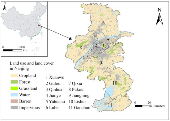
Figure 1.
Geographical location, land use, and land cover of the study area.
2.2. Data
2.2.1. Land Surface Temperature
The LST data were derived from the 1 km resolution of the monthly average temperature dataset of China, which was provided by the National Tibetan Plateau Scientific Data Center [48]. This dataset was generated in China using the Delta spatial downscaling scheme based on the global 0.5° climate dataset published by the Climatic Research Unit and the global high-resolution climate dataset published by WorldClim; the dataset was evaluated by 496 national weather stations across China, and the evaluation indicated that the downscaled dataset was reliable [49].
2.2.2. Influencing Factors
Changes in LST are the result of complex interactions between natural processes and human activities [50]. Referring to previous studies, we chose eight potential IFs that may lead to the change in LST from three categories, namely, LULC, ecological, environmental factor, and socioeconomic factor, as presented in Table 1.

Table 1.
The selected influencing factors.
- (1)
- Land Use and Land Cover
The areas of IPS and WB were derived from the 30 m LULC data of China from 2000 to 2020 [51]. To enhance objectivity, this study adopted the area ratio of IPS and WB, which was obtained by dividing the respective area by the total area of the corresponding administrative region. As mentioned above, the impact of vegetation on LST may vary under different growth states. Therefore, considering that vegetation can be characterized by NDVI, we utilized MODIS NDVI data from the MOD13A3 global dataset released by NASA instead of vegetation cover area, spanning from 2000 to 2020 and with a spatial resolution of 1 km;
- (2)
- Ecological Environmental Factor
The ecological environmental data utilized in this paper, including PREP, SSH, and near-surface RH, were sourced from the daily dataset from China’s national surface weather station data set, which has been recorded by more than 824 nationwide base and basic weather stations since 1951. Based on daily data spanning from 2000 to 2020, a raster data set with a spatial resolution of 1 km was generated using cubic spline interpolation. Subsequently, monthly data for each district in Nanjing were obtained;
- (3)
- Socioeconomic factor
The socioeconomic factors adopted in our study comprised PD and IAV. The population data were obtained from the LandScan data set. We employed a population grid data set with a spatial resolution of 1 km to estimate the annual population for each district in Nanjing between 2000 and 2020. The PD was then obtained by dividing the population of each district by the area of the corresponding district.
The IAV refers to the total industrial output minus the intermediate industrial inputs and value-added tax, which is usually used to characterize industrial output. The IAV data used in this study were derived from the China Regional Economic Statistical Yearbook and China County Statistical Yearbook. To fill in the missing values in IAV data, an autoregressive moving average model was used. Similarly, for the sake of objectivity, the IAV employed was the industrial added value within one square kilometer.
The data structures, units, and time scales of the above variables are listed in Table 1. It can be seen that the time scales of different impact factors vary. To integrate data from different time scales into seasonal data, we considered spring as March to May, summer as June to August, autumn as September to November, and winter as December to February of the following year. Since IPS, WB, PD, and IAV did not significantly differ between seasons in the same year, the annual values of these variables are used in the seasonal model. Additionally, for the variables with a monthly scale, including LST, NDVI, SSH, PREP, and RH, the seasonal value was determined by taking the average of each month within the corresponding season. Then, the number of each variable was 231 at the seasonal scale after the aforementioned processing.
3. Methodology
3.1. Generalized Additive Models (GAMs)
The generalized additive model can be expressed as the following equation:
where is the response variable; is the connection function; is the constant intercept term; is the explanatory variable; is a smoothing function for the explanatory variable that represents the linear or nonlinear relationship between response variables and explanatory variables, mainly including natural cubic spline smoothing function, local regression smoothing function, and spline smoothing function; the natural cubic spline smoothing function is employed in this study to effectively capture local variations in the data and flexibly adapt to diverse data patterns; is the total number of explanatory variables, and is a random variable that obeys normal distribution.
When exploring the causal relationship between a single explanatory variable and the response variable, the model includes only one explanatory variable, implying that there exists a sole (·) on the right-hand side of the model. When exploring the causal relationship between multiple explanatory variables and response variables, multiple explanatory variables are included at the same time; i.e., multiple functions are added on the right side of the model.
In this study, the GAMs model was built using the mgcv package in R. The F-test statistic, p-value, adjusted R-squared (adj-R2), and deviance explained (DE) given by the GAMs were used to evaluate the significance of different explanatory variables on LST and the fitted goodness of the model. Among them, the higher the F value, the stronger the significance and explanatory power; a smaller p-value typically indicates higher significance, and the closer adj-R2 is to 1, the more accurate the model is. The DE is the proportion of the null deviance explained by the model [52]. Generally speaking, the higher the DE, the greater the model-fitting effect and ability to explain it.
3.2. Mann–Kendall Trend Test
As a non-parametric method, the Mann–Kendall test (M-K test) is applicable to data distributions of all types, including data with seasonal variations. It has been extensively employed in the field of geoscience for identifying trends in time series data [11,37]. In this study, the M-K test was employed to assess the presence of any significant trends in LST from 2000 to 2020, with a significance level of 95% (p ≤ 0.05).
3.3. Correlation Analysis
In statistics, the Pearson correlation coefficient is widely used to measure the linear correlation between two variables. In this study, we utilized the Pearson correlation coefficient to characterize the linear correlation between two IFs. Pearson correlation coefficient can be expressed as follows:
where and represent the respective mean of variable and ; is the variable count. The value of falls between −1 and 1, and the bigger the absolute value, the higher the correlation between the two variables.
3.4. Akaike Information Criterion
The Akaike information criterion (AIC) [53] is a widely used method for assessing the goodness of fit of statistical models, commonly employed in model scoring and selection. In this study, AIC was employed to evaluate the goodness of fit for both the MGAMI model and MGAM model, which can be computed using the following formula [54]:
where and represent the number of parameters and the likelihood of the data in the model, respectively; represents the natural logarithm function. In general, the model with the lowest AIC is considered to be the best model [55].
3.5. Model Configurations
The IFs are embedded with correlations between each other; therefore, to quantify the effect of their interactions on LST, we conducted experiments with two configurations. One is multivariate GAMs without interactions, and the other is with interactions. Both configurations were implemented at a seasonal scale.
Concurvity, which can be viewed as an extension of co-linearity, arises when some smooth term in a model can be approximated by one or more of the other smooth terms in the model. The test of concurvity among IFs must be conducted to choose modeling factors [56]. A concurvity coefficient exceeding 0.8 indicates a high level of concurvity within the smooth term, which can potentially result in unstable parameter estimates and reduced interpretability of the model [57]. Therefore, in this study, the threshold value for the concurvity coefficient was set at 0.8. Meanwhile, the variables that did not pass the significance test were also excluded according to p-values. The final equations for the MGAM are detailed in the results section.
For the multivariate GAMs with interaction, the correlation among variables can have a significant impact on the accuracy of the model. The presence of concurvity between two explanatory variables does not necessarily preclude the possibility of a statistically significant correlation between them. The stronger the correlation between two variables, the more likely their interaction is to be. In this study, we adopted the empirical value suggested by references that problems with concurvity are likely to arise if the correlation coefficient exceeds 0.5 [56]. Therefore, in order to better characterize the impact of the interaction on LST, only variables with Pearson correlation coefficients greater than 0.5 were considered. Meanwhile, similar to the MGAM-based model, IFs with a concurvity coefficient exceeding 0.8 and those that failed the significance test were also excluded according to p-values. The final equations for multivariate GAMs with interaction are detailed in the results section.
4. Results and Analysis
4.1. Spatiotemporal Characteristics of LST
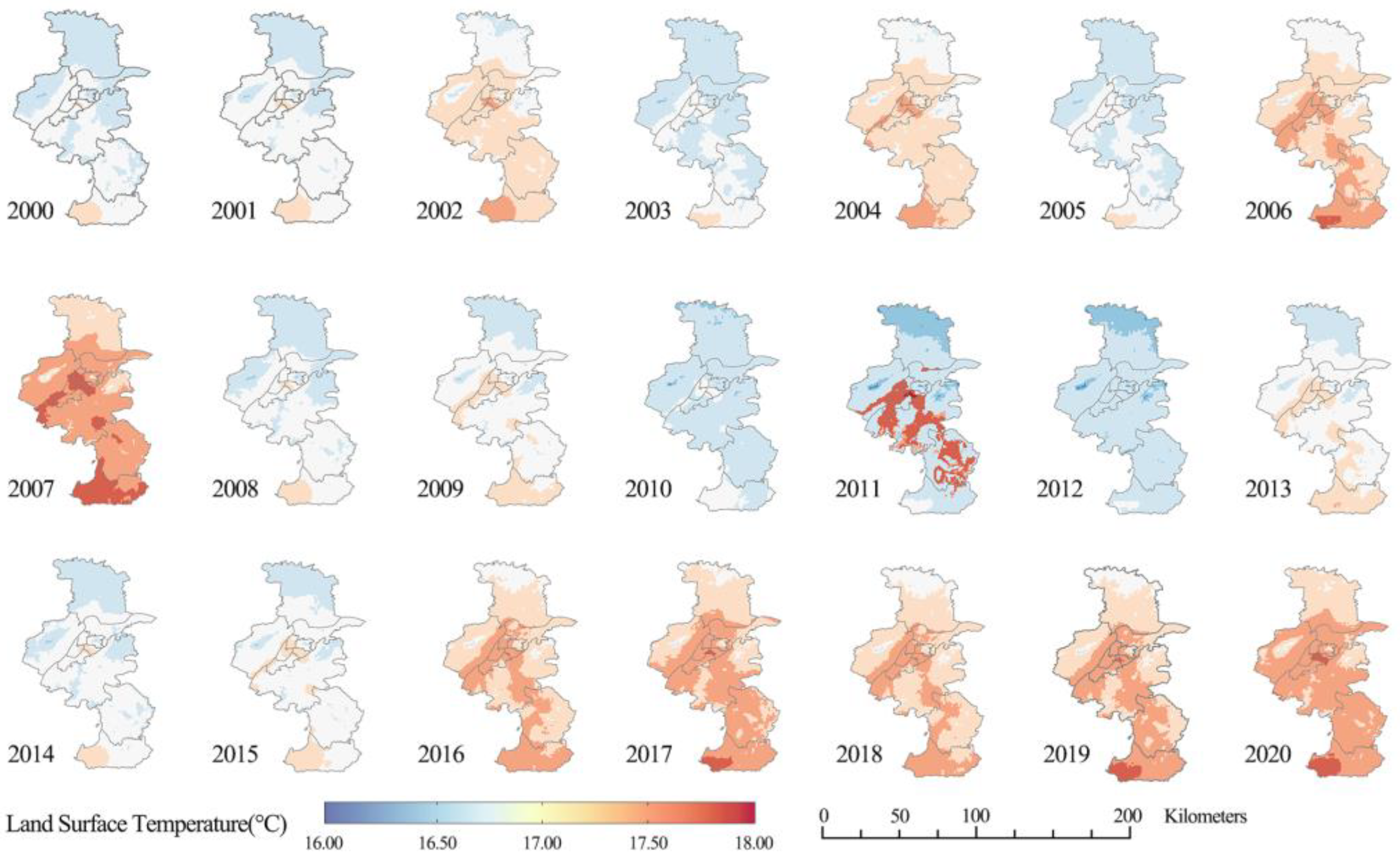
The spatiotemporal characteristics of annual mean LST (AMLST) in Nanjing from 2000 to 2020 are depicted in Figure 2. It can be seen that the AMLST mainly ranged from 14 °C to 18 °C. The lowest LST of each year occurred in the Luhe district in the north of Nanjing. The regions with higher AMLST were predominantly concentrated in Central and Southern Nanjing, where the PD and IPS were the highest, whereas the vegetation cover was the lowest. The Gaochun District, situated in the southern region of Nanjing, is predominantly an agricultural zone. Possibly attributed to the influence of relatively lower vegetation coverage and long-standing agricultural activities [58], the Gaochun district exhibited a comparatively higher AMLST in comparison to other regions within Nanjing. In addition, the LST of each district from 2000 to 2020 exhibited fluctuations rather than straight upward or downward trends. The most noticeable observation was that the LST in Central Nanjing reached its peak in 2011. Since then, the LST has fluctuated several times, showing an overall upward but not remarkable trend, and did not exceed the highest value in 2011.
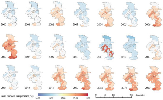
Figure 2.
Spatiotemporal variation characteristics of the annual mean land surface temperature at 1 km resolution in Nanjing from 2000 to 2020.
4.2. Temporal Trend Analysis of LST
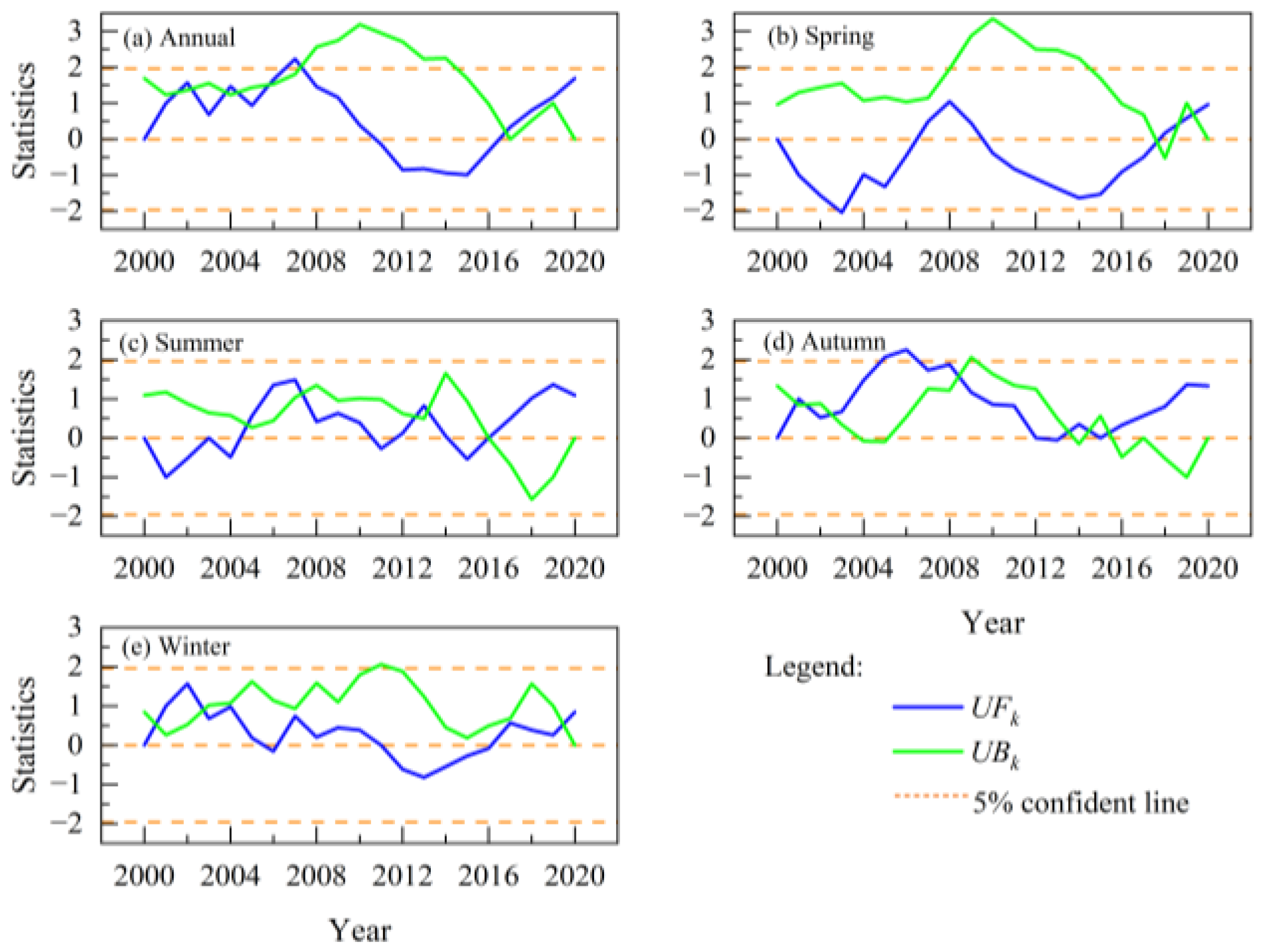
The temporal trend analysis of AMLST and seasonal mean LST (SMLST) was conducted by using the M-K test at the significance level of 95% (p ≤ 0.05). As depicted in Figure 3a, the UF value [59,60] in 2007 exceeded the confidence line (±1.96) and was greater than 0, indicating a significant rise in AMLST during that year. The UF values of other years exhibited either positive or negative, and their absolute values were both lower than 1.96, suggesting that there were insignificant upward or downward trends in the corresponding AMLST during those years.
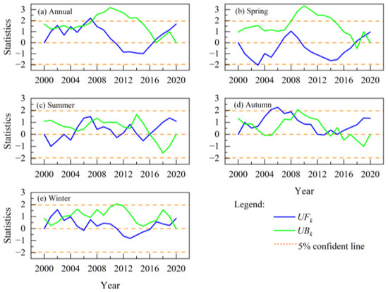
Figure 3.
MK test results of LST in Nanjing from 2000 to 2020.
The M-K test of SMLST indicated that the UF values exhibited multiple fluctuations in both summer and winter, yet all remained lower than 1.96, suggesting that the variations in SMLST during these seasons were not statistically significant. In addition, a notable decrease was observed during spring 2003, while significant increases were observed during autumn 2005 and 2006; however, no significant variation trends were observed for other years. Overall, no statistically significant changes were observed in either AMLST or SMLST.
4.3. Correlation between Influencing Factors
To provide variables for MGAMI modeling, the Pearson correlation coefficient was calculated using Equation (2) in Origin software, version 9.8.0. The results presented in Figure 4 revealed that RH, PREP, and SSH exhibited a significant correlation. Specifically, a positive correlation between RH and PREP was observed, while a negative correlation was found between SSH and both PREP and RH. The Pearson correlation coefficient between RH and SSH exhibited the highest values during spring (−0.87) and winter (−0.78), indicating a strong linear relationship between them; the lowest Pearson correlation coefficient was observed in summer (−0.67), suggesting a moderate linear relationship. The correlation between PREP and SSH exhibited a similar changing pattern. The correlation between PREP and RH exhibited seasonal variations, with the highest Pearson correlation coefficient observed in spring (0.77) and winter (0.78), while the lowest was found in summer (0.42). The Pearson correlation coefficient between IPS and IAV in summer was 0.81, which was positive and strong, and the correlation was significant.
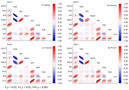
Figure 4.
Pearson correlation coefficient matrix of influencing factors.
It should be noted that all of the above correlations were significant at the significance level of 99.9% (p ≤ 0.001). In addition, under the significance levels depicted in Figure 4, several other variables also exhibited significant correlation, albeit with relatively low correlation coefficients. The subsequent studies aimed to investigate the effect of the interaction between IFs on LST, and only IFs with a Pearson correlation coefficient exceeding 0.5 were considered.
4.4. Results of Multivariate GAMs (MGAM)
The concurvity coefficient can be measured by using the concurvity function in the mgcv package. As mentioned in the Methodology section, the threshold value for the concurvity coefficient was set at 0.8. Meanwhile, the variables that did not pass the significance test were also excluded from the modeling. We also conducted the multicollinearity test using the Variance Inflation Factor, and the results showed that there was no multicollinearity among the remaining variables. Perhaps this is because concurvity can be seen as the nonlinear form of collinearity. The final equations for each season were, thus, as follows:
where s () is regular smooth terms, which can describe the linear and nonlinear relations between the independent variable and the dependent variable [52]; is the count of basic functions, which can be determined by examining the checking the results of basis dimension.
The modeling results based on MGAM are presented in Table 2. According to the p-value results, the effect of each variable on LST was statistically significant. DEs of the summer model (83.7%) and winter model (70.6%) were relatively high, followed by the autumn model (67.0%) and spring model (59.2%). The variation pattern of adj-R2 was similar to that of DE, with the highest adj-R2 observed in the summer model (0.816), followed by the winter model (0.672), autumn model (0.628), and spring model (0.537). The above findings indicated that the summer model exhibited superior performance in describing the variation in LST, while the spring model demonstrated relatively poorer performance.
Table 2.
Results of the Multivariate GAMs without interaction.
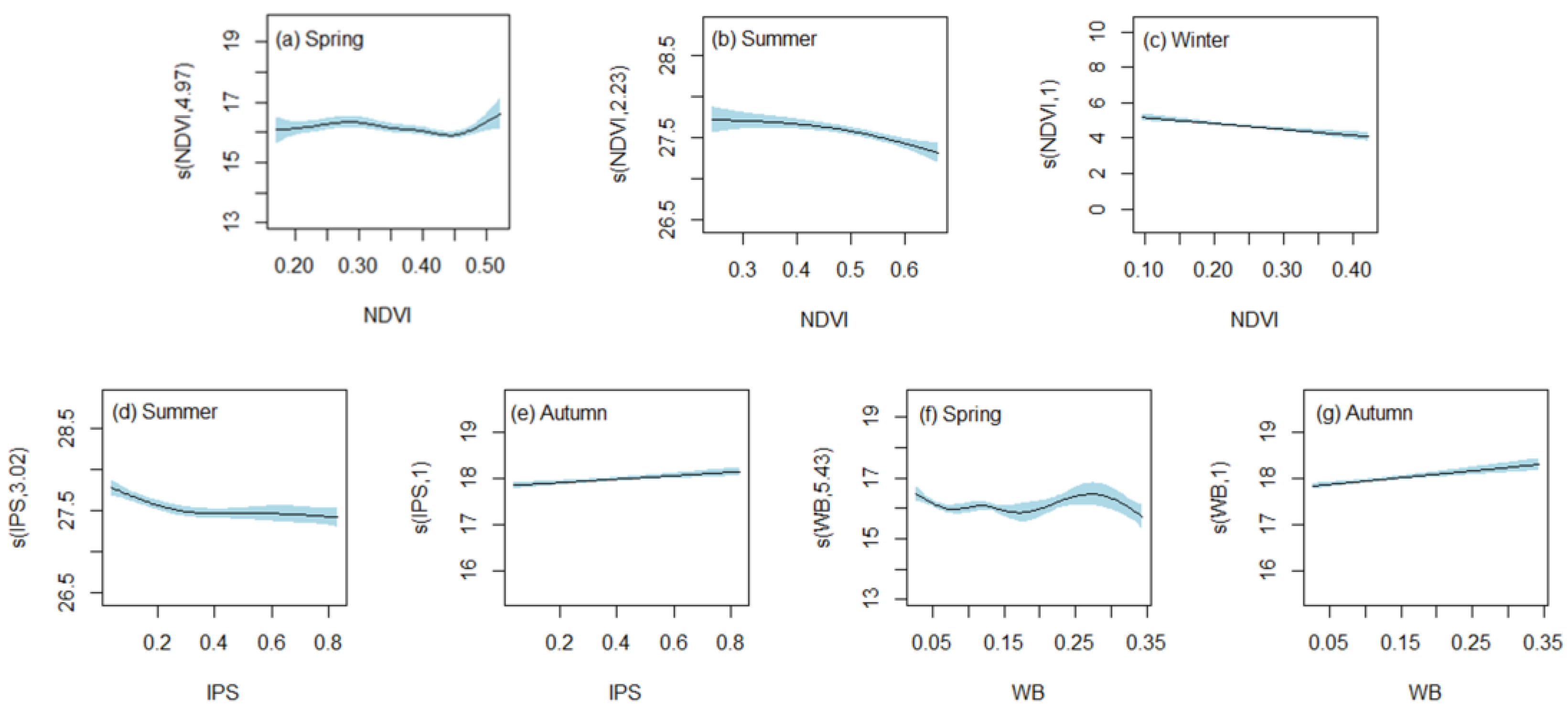
According to the value of effective degrees of freedom (edf) given by GAMs, the action mode (linear or nonlinear) can be determined. An edf of 1 indicates that the effect of the influence factor on LST is linear, and otherwise, it is nonlinear. Based on Table 2, it can be inferred that the edf of NDVI in both spring and summer models was greater than 1, indicating a nonlinear correlation between NDVI and LST. This nonlinear correlation can also be observed in Figure 5a,b. In spring, the relationship between NDVI and LST was found to be more complex, suggesting that vegetation did not have a simple warming or cooling effect on LST. However, vegetation exerted a nonlinear cooling effect on LST in summer. In addition, as shown in Figure 5c, the relationship between NDVI and LST in winter exhibited a negative linear correlation, indicating that vegetation had a significant cooling effect on LST.
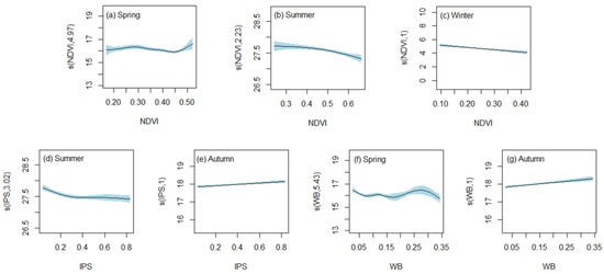
Figure 5.
The estimated effects of NDVI, IPS, and WB with 95% confidence bands. The shade represents the confidence interval; the solid line represents the smooth fitting curve. The numbers in parentheses on the ordinate represent the estimated degrees of freedom.
In a multivariate GAMs model, the estimated effects are used to represent the influence of a single variable on the response variable. In this study, the estimated effects of IPS on LST were found to be statistically significant in both the summer and autumn at a significance level of 100%. In the summer model, the edf of IPS was 3.020, indicating a nonlinear relationship between IPS and LST, as shown in Figure 5d. Conversely, in the autumn model, the edf of IPS was close to 1, suggesting an approximately linear relationship between IPS and LST, which was further confirmed in Figure 5e. Moreover, the positive slope of the solid line indicated that IPS had a warming effect on LST.
The estimated effects of WB on LST were significant in both spring model and autumn model at the significance level of 99.9% and 100%, respectively. Furthermore, as depicted in Figure 5f,g, the influence of WB on LST was observed nonlinear in spring, whereas it was linear in autumn. In addition, the WB exhibited a warming effect on LST during autumn, while in spring, it functioned as a thermostat for LST by maintaining it at approximately 16 °C.
The importance and explanatory ability (IEA) of each explanatory variable to the response variable can be quantified by GAMs through the value of the F-test statistic. As illustrated in Table 2, the IEA of each explanatory variable varied with seasons. In spring, the IEA of SSH was strongest, followed by RH, PREP, WB, and NDVI. Compared with other seasonal models, the summer model had a larger DE and adj-R2 and possessed the best ability to describe changes in LST. The order of decreasing IEA was SSH, RH, NDVI, PREP, and IPS. The autumn model was better than the spring model at describing the change pattern of LST. The factor with the highest IEA in the autumn model was WB, while RH had the lowest IEA. In winter, SSH made the greatest contribution, followed by NDVI, whereas RH and PREP made relatively minor contributions.
The results presented in Table 2 demonstrated the significant and nonlinear influence of SSH, RH, and PREP on LST in all four seasons. According to the correlation analysis in Section 4.3, it was observed that RH exhibited a significant positive correlation with PREP, while SSH displayed a significant negative correlation with both RH and PREP. Consequently, their impact on LST could either mutually constrain or reinforce each other, making it challenging to elucidate their respective influences on LST. For instance, an increase in PREP does not necessarily imply a decrease in LST due to the complex relationship among SSH, RH, and PREP.
4.5. Results of Multivariate GAMs with Interaction (MGAMI)
Taking into account the concurvity, linear correlation, and significance, the following equations were ultimately used to represent the relationship between LST and IFs for each season:
where is regular smooth terms; represents tensor smooth functions designed to model the interaction effects among two variables [52]; is the number of basic functions.
The results from the modeling are presented in Table 3. According to the p-value column, the estimated effects of IFs above on LST were found to be statistically significant at the significance level of 99.9% or 100%.
Table 3.
Results of the Multivariate GAMs with interaction.
The smooth terms mentioned above are visualized in Figure 6. In multivariate GAMs with interaction (MGAMI), the relationship between NDVI and LST exhibited a nonlinear trend. Figure 6a demonstrated that the impact of NDVI on LST was influenced by the variation in vegetation cover during spring, displaying a pattern of warming–cooling–warming. During the summer season, NDVI exhibited a positive correlation with LST when its values were below 0.32; conversely, NDVI with higher values had a cooling effect on the land surface. Throughout the entire winter (Figure 6c), NDVI consistently acted as a cooling agent.
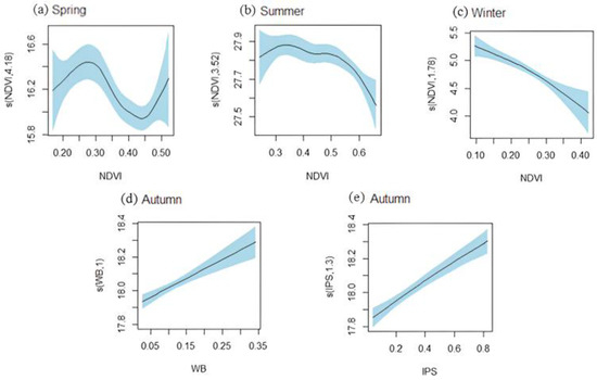
Figure 6.
The estimated effects (ESTE) of the explanatory variables on LST with 95% confidence bands: (a) The ESTE of NDVI in spring; (b) The ESTE of NDVI in summer; (c) The ESTE of NDVI in winter; (d) The ESTE of WB in autumn; (e) The ESTE of IPS in autumn. The shade represents the confidence interval, while the solid line represents the smooth fitting curve. The numbers in parentheses on the ordinate indicate the estimated degrees of freedom.
As shown in Table 3 and Figure 6e, the edf of IPS in autumn was 1, and the slope of the solid line was greater than 0, indicating that IPS had a significant warming effect on the land surface, which was similar to that observed in autumn model without interaction terms. In autumn (Figure 6d), the warming effect of WB on LST exhibited a significant linear trend, which was consistent with the findings from GAMs without interaction terms (Figure 5g). Moreover, the Pearson correlation coefficients between LST and both WB and IPS were positive at 0.2, indicating a significant positive relationship at the 99% significance level, which could partially explain the correctness of the results.
The estimated effects of the interactive terms are illustrated in Figure 7. As shown in the figure, the X and Y axes represent two variables with significant interaction, respectively. The Z-axis represents the estimated LST corresponding to the interaction between the variables. The arrow indicates the direction in which the value increases. Due to the significant variations in SSH, RH, and PREP across different seasons, the influence pattern of the interactions between the same two IFs exhibited seasonal disparities. For example, the impact of the interaction between RH and PREP varied between spring, autumn, and winter models. In addition, the significant IFs varied across seasons. In spring, the changes in LST were primarily influenced by the interaction between RH and PREP, in addition to the impact of NDVI. The significantly interactive factors observed during the summer period encompassed SSH-PREP and SSH-RH. The significantly interactive factors in autumn and winter remained consistent, encompassing both SSH-PREP and RH-PREP. It was worth noting that the influence of the interaction in the four seasons was all nonlinear. Additionally, it seemed easier to understand the variation pattern of LST after considering the effect of the interaction terms. For instance, Figure 7a illustrates that in the spring model, when PREP was almost at its minimum, and RH was almost at 62.94%, the estimated LST corresponding to the interaction between RH and PREP almost reached its lowest point. In the autumn model, Figure 7e demonstrates that when both PREP and RH reached their maximum values, the estimated LST of the interaction between RH and PREP almost also reached its minimum value. The reason may be that high precipitation can lead to an increase in relative humidity, which often results in the formation of clouds [61]. Clouds have the ability to reflect and scatter solar radiation, thereby reducing the amount of solar radiation reaching the ground and consequently lowering LST. Similarly, Figure 7g showed that in the winter model, when PREP reached its minimum, and RH reached its maximum, the interaction between RH and PREP resulted in the smallest estimated LST. For a similar reason, high relative humidity eventually reduces the amount of solar radiation reaching the surface, resulting in lower surface temperatures. Additionally, the interaction between SSH and PREP exhibited a similar impact on LST in the autumn model (Figure 7f) and the winter model (Figure 7d), except for the summer model presented in Figure 7b.
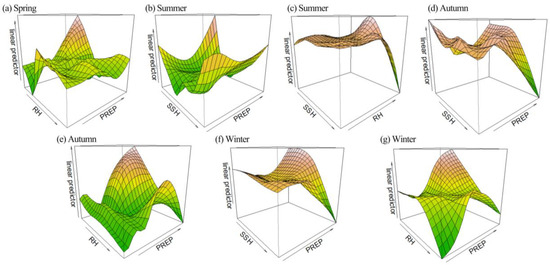
Figure 7.
The effect of interactions (EOI) of explanatory variables on LST: (a) The EOI of RH and PREP in spring; (b) The EOI of SSH and PREP in summer; (c) The EOI of SSH and RH in summer; (d) The EOI of SSH and PREP in autumn; (e) The EOI of RH and PREP in autumn; (f) The EOI of SSH and PREP in winter; (g) The EOI of RH and PREP in winter. The colors represent the predicted LST values, with green indicating lower values and red indicating higher values.
5. Discussion
Accurately revealing the driving factors of LST is helpful for scientifically formulating measures to address climate warming [3,62]. In this study, eight potential influencing factors were used as explanatory variables to elucidate the mechanism of the changes in LST. Correlation analysis revealed significant correlations between IPS and IAV, IPS and NDVI, SSH and PREP, as well as RH and PREP. However, the majority of existing studies tended to overlook the impact of interactions between IFs on the changes in LST, which could damage the modeling accuracy and lead to potentially biased conclusions. Therefore, in order to accurately identify the influencing factors of LST based on the advantages of GAMs and consider correlation, concurvity, and significance comprehensively, we ultimately established four models to reveal the causes of LST changes at a seasonal scale. The modeling results indicated that the variables IAV, PD, the interaction between IPS and IAV, as well as the interaction between IPS and NDVI did not exert a statistically significant influence on LST.
The model accuracy is found to be enhanced by taking into account the interaction between IFs, as evidenced by our experimental findings. The comparison of Table 2 and Table 3 reveals that DE and adj-R2 of different MGAMI-based seasonal models have been increased to some extent, indicating that the models based on MGAMI could better describe the changes in LST. As depicted in Figure 8, the autumn model exhibited the most significant improvement, with an increase of 17.9% and 0.19 for DE and adj-R2, respectively. Followed by the winter model, DE and adj-R2 improved by 15.4% and 0.15. The spring model showed the least improvement, with DE and adj-R2 increasing by 2.3% and 0.02, respectively. Furthermore, the root mean square error (RMSE) and mean absolute error (MAE) of the difference between LST and the fitted value have also been improved to varying degrees. The improvement was most significant in winter, followed by autumn, summer, and spring. Compared with MGAM, RMSE, and MAE of MGAMI decreased by 0.173 °C and 0.150 °C, respectively, in winter and decreased by 0.012 °C and 0.018 °C, respectively, in spring.
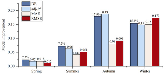
Figure 8.
The improvement in the seasonal GAMs model considering the interaction between variables (DE: Deviance explained; adj-R2: adjusted R-squared).
To further evaluate the model’s performance, we calculated the AIC of MGAM and MGAMI models for each season, and the results are presented in Table 4.
Table 4.
AIC results of seasonal models.
As shown in Table 4, the AIC of the MGAMI seasonal model both decreased to varying degrees compared to the MGAM seasonal model, with the largest decrease observed in the autumn model, followed by winter, summer, and spring models. The improvement pattern observed was similar to that shown in Figure 8. The comparison results of AIC further confirmed that considering the interaction between variables can improve the goodness of fit.
Furthermore, MGAMI could produce more accurate modeling results by considering the interaction between IFs. In the MGAM-based summer model, IPS showed a slight cooling effect on the surface, which may not be consistent with reality. By comparing Table 2 and Table 3, it could be seen that when considering the interactions between IFs in the summer model, the cooling impact of IPS on LST became insignificant. On the contrary, as shown in Figure 6e, IPS exhibited a significant warming effect on the land surface in the autumn model based on MGAMI, which was more consistent with the findings reported in the literature [12,63]. It was also found that the significant effect of WB disappeared in the spring model based on MGAM when considering the influence of interactions between IFs. As depicted in Figure 6d, WB had a significant warming effect on the land surface in the autumn model based on MGAMI, which was consistent with the conclusion presented in previous studies [15]. Both SHH, RH, and PREP and the interactions between them exhibited significant and nonlinear effects on LST. The importance of the interaction between SHH, RH, and PREP varied seasonally, which might be associated with seasonal fluctuations in sunshine hours, relative humidity, precipitation, and NDVI.
Also, the models based on MGAM and MGAMI yielded some similar conclusions. Similar to the conclusion of Meng et al. [15], the influence of NDVI on LST exhibited seasonal differences. During spring, the relationship between NDVI and LST displayed nonlinearly in response to vegetation growth, resulting in both warming and cooling effects on LST. Conversely, vegetation primarily exerted a cooling effect on LST during summer and winter.
6. Conclusions
The variation in LST is the result of multiple factors functioning together. Various IFs exhibit seasonal and spatial differences in their impacts on LST. In this study, we employed the Generalized Additive Model to explore the impacts of the IFs and their interactions on the variation in LST in Nanjing spanning from 2000 to 2020. To further explore the interactions between IFs and LST, we complemented the experiments with two configurations of GAMs, i.e., considering and not considering the interactions between IFs.
Results showed that the spatial difference in annual mean land surface temperature in Nanjing was evident, with higher temperatures observed in the central and southern regions compared to the northern areas. Overall, there was no significant upward trend in season mean land surface temperature.
With GAMs, the significance, action mode, action effect, and the order of importance of IFs on LST can be easily identified. According to the results of MGAMI, vegetation primarily played a cooling role in LST, while impervious surfaces contributed to warming LST. Most importantly, at the 100% significance level, the interaction among SSH, RH, and PREP had a significant impact on LST. It was also worth noting that certain IFs underwent a transition from significant to non-significant impact after considering the interaction of IFs. The goodness of fit and interpretability of the model could be significantly enhanced by MGAMI compared to MGAM.
In view of these results, this study suggests the following proposals. In order to more accurately reveal the factors influencing LST and predict future LST, it is suggested that a single factor is not enough, but the interactions are more important for a comprehensive understanding of the LST. With rapid urbanization, the impervious surface is increasing rapidly, which poses a threat to the environment and climate. Therefore, policymakers should combine the research results to develop reasonable, sustainable development measures to deal with the problem of climate warming. For instance, the relevant departments should strategically organize the implementation of afforestation to enhance the urban vegetation coverage, thereby harnessing the cooling effect of vegetation to counterbalance the rise in LST resulting from impervious surfaces.
Author Contributions
Conceptualization, X.Z.; investigation, X.Z. and F.Y.; methodology, X.Z. and F.Y.; visualization, X.Z. and F.Y.; writing—original draft, X.Z. and F.Y.; writing—review and editing, J.Z. and Q.D. All authors have read and agreed to the published version of the manuscript.
Funding
This work was supported by the innovative training project for college students [grant number 202310319128Y].
Data Availability Statement
Publicly available data sets were analyzed in this study. LST data are available at http://data.tpdc.ac.cn/ (accessed on 14 July 2023); LULC data are available at https://zenodo.org/record/8176941 (accessed on 18 July 2023); NDVI data can be download at https://search.earthdata.nasa.gov (accessed on 25 July 2023); PREP, SSH and RH data are available at http://101.200.76.197:93/ (accessed on 25 July 2023); The population data are available at https://landscan.ornl.gov (accessed on 28 July 2023).
Conflicts of Interest
The authors declare no conflict of interest.
References
- Jiang, K.; Pan, Z.; Pan, F.; Teuling, A.J.; Han, G.; An, P.; Chen, X.; Wang, J.; Song, Y.; Cheng, L.; et al. Combined influence of soil moisture and atmospheric humidity on land surface temperature under different climatic background. iScience 2023, 26, 106837. [Google Scholar] [CrossRef] [PubMed]
- Yu, Y.; Duan, S.B.; Li, Z.L.; Chang, S.; Xing, Z.; Leng, P.; Gao, M. Interannual Spatiotemporal Variations of Land Surface Temperature in China From 2003 to 2018. IEEE J. Sel. Top. Appl. Earth Obs. Remote Sens. 2021, 14, 1783–1795. [Google Scholar] [CrossRef]
- Yu, Y.; Fang, S.; Zhuo, W. Revealing the Driving Mechanisms of Land Surface Temperature Spatial Heterogeneity and Its Sensitive Regions in China Based on GeoDetector. Remote Sens. 2023, 15, 2814. [Google Scholar] [CrossRef]
- Li, Z.-L.; Tang, B.-H.; Wu, H.; Ren, H.; Yan, G.; Wan, Z.; Trigo, I.F.; Sobrino, J.A. Satellite-derived land surface temperature: Current status and perspectives. Remote Sens. Environ. 2013, 131, 14–37. [Google Scholar] [CrossRef]
- Yang, C.; Yan, F.; Lei, X.; Ding, X.; Zheng, Y.; Liu, L.; Zhang, S. Investigating Seasonal Effects of Dominant Driving Factors on Urban Land Surface Temperature in a Snow-Climate City in China. Remote Sens. 2020, 12, 3006. [Google Scholar] [CrossRef]
- Garzón, J.; Molina, I.; Velasco, J.; Calabia, A. A Remote Sensing Approach for Surface Urban Heat Island Modeling in a Tropical Colombian City Using Regression Analysis and Machine Learning Algorithms. Remote Sens. 2021, 13, 4256. [Google Scholar] [CrossRef]
- Liu, M.; Ma, H.; Bai, Y. Understanding the Drivers of Land Surface Temperature Based on Multisource Data: A Spatial Econometric Perspective. IEEE J. Sel. Top. Appl. Earth Obs. Remote Sens. 2021, 14, 12263–12272. [Google Scholar] [CrossRef]
- Liu, K.; Li, X.; Wang, S.; Li, Y. Investigating the impacts of driving factors on urban heat islands in southern China from 2003 to 2015. J. Clean. Prod. 2020, 254, 120141. [Google Scholar] [CrossRef]
- Joly, D.; Bois, B.; Zakšek, K. Rank-Ordering of topographic variables correlated with temperature. Atmos. Clim. Sci. 2012, 2, 139–147. [Google Scholar] [CrossRef]
- Min, M.; Lin, C.; Duan, X.; Jin, Z.; Zhang, L. Spatial distribution and driving force analysis of urban heat island effect based on raster data: A case study of the Nanjing metropolitan area, China. Sustain. Cities Soc. 2019, 50, 101637. [Google Scholar] [CrossRef]
- Zhou, S.; Liu, D.; Zhu, M.; Tang, W.; Chi, Q.; Ye, S.; Xu, S.; Cui, Y. Temporal and Spatial Variation of Land Surface Temperature and Its Driving Factors in Zhengzhou City in China from 2005 to 2020. Remote Sens. 2022, 14, 4281. [Google Scholar] [CrossRef]
- Wu, Z.; Yao, L.; Zhuang, M.; Ren, Y. Detecting factors controlling spatial patterns in urban land surface temperatures: A case study of Beijing. Sustain. Cities Soc. 2020, 63, 102454. [Google Scholar] [CrossRef]
- Guo, J.; Han, G.; Xie, Y.; Cai, Z.; Zhao, Y. Exploring the relationships between urban spatial form factors and land surface temperature in mountainous area: A case study in Chongqing city, China. Sustain. Cities Soc. 2020, 61, 102286. [Google Scholar] [CrossRef]
- Gunawardena, K.R.; Wells, M.J.; Kershaw, T. Utilising green and bluespace to mitigate urban heat island intensity. Sci. Total Environ. 2017, 584–585, 1040–1055. [Google Scholar] [CrossRef] [PubMed]
- Meng, Q.; Liu, W.; Zhang, L.; Allam, M.; Bi, Y.; Hu, X.; Gao, J.; Hu, D.; Jancsó, T. Relationships between Land Surface Temperatures and Neighboring Environment in Highly Urbanized Areas: Seasonal and Scale Effects Analyses of Beijing, China. Remote Sens. 2022, 14, 4340. [Google Scholar] [CrossRef]
- Peng, J.; Jia, J.; Liu, Y.; Li, H.; Wu, J. Seasonal contrast of the dominant factors for spatial distribution of land surface temperature in urban areas. Remote Sens. Environ. 2018, 215, 255–267. [Google Scholar] [CrossRef]
- Abbas, A.; He, Q.; Jin, L.L.; Li, J.L.; Salam, A.; Lu, B.; Yasheng, Y. Spatio-Temporal Changes of Land Surface Temperature and the Influencing Factors in the Tarim Basin, Northwest China. Remote Sens. 2021, 13, 3792. [Google Scholar] [CrossRef]
- Nabizada, A.F.; Rousta, I.; Dalvi, M.; Olafsson, H.; Siedliska, A.; Baranowski, P.; Krzyszczak, J. Spatial and Temporal Assessment of Remotely Sensed Land Surface Temperature Variability in Afghanistan during 2000–2021. Climate 2022, 10, 111. [Google Scholar] [CrossRef]
- Tian, H.; Liu, L.; Zhang, Z.; Chen, H.; Zhang, X.; Wang, T.; Kang, Z. Spatiotemporal diversity and attribution analysis of land surface temperature in China from 2001 to 2020. Acta Geogr. Sin. 2022, 77, 1713–1729. [Google Scholar]
- Yao, T.D.; Jiao, K.Q.; Yang, M. Precipitation variations recorded in Guliya ice core in the past 400 years. Prog. Nat. Sci. 2000, 10, 292–293. [Google Scholar]
- Littmann, T. Rainfall, Temperature and Dust Storm Anomalies in the African Sahel. Geogr. J. 1991, 157, 136–160. [Google Scholar] [CrossRef]
- Duan, K.; Yao, T.; Thompson, L.G. Response of monsoon precipitation in the Himalayas to global warming. J. Geophys. Res. Atmos. 2006, 111, D19110. [Google Scholar] [CrossRef]
- Aigang, L. Precipitation effects on temperature—A case study in China. J. Earth Sci. 2011, 22, 792–798. [Google Scholar] [CrossRef]
- Kauppinen, J.; Heinonen, J.; Malmi, P. Influence of Relative Humidity and Clouds on the Global Mean Surface Temperature. Energy Environ. 2014, 25, 389–399. [Google Scholar] [CrossRef]
- Ji, Y.; Peng, Y.; Li, Z.; Li, J.; Liu, S.; Cai, X.; Yin, Y.; Feng, T. Driving Mechanism of Differentiation in Urban Thermal Environment during Rapid Urbanization. Remote Sens. 2023, 15, 2075. [Google Scholar] [CrossRef]
- Rongbo, X.; Ouyang, Z.; Li, W.; Schienke, E.; Zhang, Z. Land Surface Temperature Variation and Major Factors in Beijing, China. Photogramm. Eng. Remote Sens. 2008, 74, 451–461. [Google Scholar] [CrossRef]
- Song, Z.; Yang, H.; Huang, X.; Yu, W.; Huang, J.; Ma, M. The spatiotemporal pattern and influencing factors of land surface temperature change in China from 2003 to 2019. Int. J. Appl. Earth Obs. Geoinf. 2021, 104, 102537. [Google Scholar] [CrossRef]
- Chen, X.; Yang, L. Temperature and industrial output: Firm-level evidence from China. J. Environ. Econ. Manag. 2019, 95, 257–274. [Google Scholar] [CrossRef]
- Tao, A.X. Study on Environment Engineering with Influence of Human Factors on the Temperature Variation in Beijing City. Adv. Mater. Res. 2013, 788, 400–404. [Google Scholar] [CrossRef]
- Peng, X.; Wu, W.; Zheng, Y.; Sun, J.; Hu, T.; Wang, P. Correlation analysis of land surface temperature and topographic elements in Hangzhou, China. Sci. Rep. 2020, 10, 10451. [Google Scholar] [CrossRef] [PubMed]
- Guo, Y.; Zhang, C. Analysis of Driving Force and Driving Mechanism of the Spatial Change of LST Based on Landsat 8. J. Indian Soc. Remote Sens. 2022, 50, 1787–1801. [Google Scholar] [CrossRef]
- He, J.; Zhao, W.; Li, A.; Wen, F.; Yu, D. The impact of the terrain effect on land surface temperature variation based on Landsat-8 observations in mountainous areas. Int. J. Remote Sens. 2019, 40, 1808–1827. [Google Scholar] [CrossRef]
- Rao, Y.; Dai, J.; Dai, D.; He, Q. Effect of urban growth pattern on land surface temperature in China: A multi-scale landscape analysis of 338 cities. Land. Use Policy 2021, 103, 105314. [Google Scholar] [CrossRef]
- Jung, M.C.; Dyson, K.; Alberti, M. Urban Landscape Heterogeneity Influences the Relationship between Tree Canopy and Land Surface Temperature. Urban. For. Urban. Green. 2021, 57, 126930. [Google Scholar] [CrossRef]
- Xi, M.; Zhang, W.; Li, W.; Liu, H.; Zheng, H. Distinguishing Dominant Drivers on LST Dynamics in the Qinling-Daba Mountains in Central China from 2000 to 2020. Remote Sens. 2023, 15, 878. [Google Scholar] [CrossRef]
- Zhao, W.; Duan, S.-B.; Li, A.; Yin, G. A practical method for reducing terrain effect on land surface temperature using random forest regression. Remote Sens. Environ. 2019, 221, 635–649. [Google Scholar] [CrossRef]
- Hou, H.; Su, H.; Liu, K.; Li, X.; Chen, S.; Wang, W.; Lin, J. Driving forces of UHI changes in China's major cities from the perspective of land surface energy balance. Sci. Total Environ. 2022, 829, 154710. [Google Scholar] [CrossRef] [PubMed]
- Wu, X.; Wang, L.; Yao, R.; Luo, M.; Li, X. Identifying the dominant driving factors of heat waves in the North China Plain. Atmos. Res. 2021, 252, 105458. [Google Scholar] [CrossRef]
- de Brogniez, D.; Ballabio, C.; Stevens, A.; Jones, R.J.A.; Montanarella, L.; van Wesemael, B. A map of the topsoil organic carbon content of Europe generated by a generalized additive model. Eur. J. Soil Sci. 2015, 66, 121–134. [Google Scholar] [CrossRef]
- Ma, Y.; Ma, B.; Jiao, H.; Zhang, Y.; Xin, J.; Yu, Z. An analysis of the effects of weather and air pollution on tropospheric ozone using a generalized additive model in Western China: Lanzhou, Gansu. Atmos. Environ. 2020, 224, 117342. [Google Scholar] [CrossRef]
- Ascensão, F.; Ribeiro, Y.G.G.; Campos, Z.; Yogui, D.R.; Desbiez, A.L.J. Forecasting seasonal peaks in roadkill patterns for improving road management. J. Environ. Manag. 2022, 321, 115903. [Google Scholar] [CrossRef] [PubMed]
- Becker, N.; Rust, H.; Ulbrich, U. Weather impacts on various types of road crashes: A quantitative analysis using generalized additive models. Eur. Transp. Res. Rev. 2022, 14, 37. [Google Scholar] [CrossRef]
- Dastoorpoor, M.; Khanjani, N.; Moradgholi, A.; Sarizadeh, R.; Cheraghi, M.; Estebsari, F. Correction to: Prenatal exposure to ambient air pollution and adverse pregnancy outcomes in Ahvaz, Iran: A generalized additive model. Int. Arch. Occup. Environ. Health 2022, 95, 1805. [Google Scholar] [CrossRef] [PubMed]
- Dominici, F.; McDermott, A.; Zeger, S.L.; Samet, J.M. On the Use of Generalized Additive Models in Time-Series Studies of Air Pollution and Health. Am. J. Epidemiol. 2002, 156, 193–203. [Google Scholar] [CrossRef] [PubMed]
- Hart, R.; Pedersen, W.; Skardhamar, T. Blowing in the wind? Testing the effect of weather on the spatial distribution of crime using Generalized Additive Models. Crime. Sci. 2022, 11, 9. [Google Scholar] [CrossRef] [PubMed]
- Khoda Bakhshi, A.; Ahmed, M.M. Real-time crash prediction for a long low-traffic volume corridor using corrected-impurity importance and semi-parametric generalized additive model. J. Transp. Saf. Secur. 2022, 14, 1165–1200. [Google Scholar] [CrossRef]
- Zhang, Y.; Zhou, R.; Hu, D.; Chen, J.; Xu, L. Modelling driving factors of PM2.5 concentrations in port cities of the Yangtze River Delta. Mar. Pollut. Bull. 2022, 184, 114131. [Google Scholar] [CrossRef] [PubMed]
- Peng, S. 1-km Monthly Mean Temperature Dataset for China (1901–2022). 2020. Available online: https://cstr.cn/18406.11.Meteoro.tpdc.270961 (accessed on 14 July 2023).
- Peng, S.; Ding, Y.; Liu, W.; Li, Z. 1 km monthly temperature and precipitation dataset for China from 1901 to 2017. Earth Syst. Sci. Data 2019, 11, 1931–1946. [Google Scholar] [CrossRef]
- Stott, P.A.; Tett, S.F.B.; Jones, G.S.; Allen, M.R.; Mitchell, J.F.B.; Jenkins, G.J. External Control of 20th Century Temperature by Natural and Anthropogenic Forcings. Science 2000, 290, 2133–2137. [Google Scholar] [CrossRef] [PubMed]
- Yang, J.; Huang, X. The 30 m annual land cover dataset and its dynamics in China from 1990 to 2021. Earth Syst. Sci. Data 2022, 13, 3907–3925. [Google Scholar] [CrossRef]
- Wood, S.N. Generalized Additive Models: An Introduction with R, 2nd ed.; Chapman and Hall/CRC: Boca Raton, FL, USA, 2017. [Google Scholar]
- Akaike, H. A new look at the statistical model identification. IEEE Trans. Autom. Control 1974, 19, 716–723. [Google Scholar] [CrossRef]
- Sutherland, C.; Hare, D.; Johnson, P.J.; Linden, D.W.; Montgomery, R.A.; Droge, E. Practical advice on variable selection and reporting using Akaike information criterion. Proc. R. Soc. B-Biol. Sci. 2023, 290, 20231261. [Google Scholar] [CrossRef] [PubMed]
- Burnham, K.P.; Anderson, D.R. Advanced Issues and Deeper Insights. In Model Selection and Multimodel Inference: A Practical Information-Theoretic Approach; Springer: New York, NY, USA, 2002. [Google Scholar]
- Ramsay, T.O.; Burnett, R.T.; Krewski, D. The effect of concurvity in generalized additive models linking mortality to ambient particulate matter. Epidemiology 2003, 14, 18–23. [Google Scholar] [CrossRef] [PubMed]
- Ross, N. Generalized Additive Models in R: A Free Interactive Course. Available online: https://noamross.github.io/gams-in-r-course/ (accessed on 10 March 2024).
- Zhou, D.; Xiao, J.; Frolking, S.; Liu, S.; Zhang, L.; Cui, Y.; Zhou, G. Croplands intensify regional and global warming according to satellite observations. Remote Sens. Environ. 2021, 264, 112585. [Google Scholar] [CrossRef]
- Zhu, M.; Liu, D.; Tang, W.; Chi, Q.; Zhao, X.; Xu, S.; Ye, S.; Wang, Y.; Cui, Y.; Zhou, S. Exploring the Ecological Climate Effects Based on Five Land Use Types: A Case Study of the Huang-Huai-Hai River Basin in China. Land 2022, 11, 265. [Google Scholar] [CrossRef]
- Malik, A.; Kumar, A.; Guhathakurta, P.; Kisi, O. Spatial-temporal trend analysis of seasonal and annual rainfall (1966–2015) using innovative trend analysis method with significance test. Arab. J. Geosci. 2019, 12, 328. [Google Scholar] [CrossRef]
- Walcek, C. Cloud Cover and Its Relationship to Relative Humidity during a Springtime Midlatitude Cyclone. Mon. Weather. Rev. -Mon. Weather. Rev. 1994, 122, 1021–1035. [Google Scholar] [CrossRef]
- He, Z.W.; Tang, B.H. Spatiotemporal change patterns and driving factors of land surface temperature in the Yunnan-Kweichow Plateau from 2000 to 2020. Sci. Total Environ. 2023, 896, 165288. [Google Scholar] [CrossRef] [PubMed]
- Ma, X.; Peng, S. Assessing the quantitative relationships between the impervious surface area and surface heat island effect during urban expansion. PeerJ 2021, 9, e11854. [Google Scholar] [CrossRef] [PubMed]


Disclaimer/Publisher’s Note: The statements, opinions and data contained in all publications are solely those of the individual author(s) and contributor(s) and not of MDPI and/or the editor(s). MDPI and/or the editor(s) disclaim responsibility for any injury to people or property resulting from any ideas, methods, instructions or products referred to in the content. |
© 2024 by the authors. Licensee MDPI, Basel, Switzerland. This article is an open access article distributed under the terms and conditions of the Creative Commons Attribution (CC BY) license (https://creativecommons.org/licenses/by/4.0/).