Spatial–Temporal Pattern of Coordination between the Supply and Demand for Ecosystem Services in the Lhasa River Basin

Abstract

Quantifying the spatiotemporal patterns of the coordination between ecosystem service supply and demand is vital for regional sustainable development. To reveal the dynamic pattern of the coordination of ecosystem service (ES) supply and demand in the Lhasa River Basin, we quantified the supply of the following four ESs using the InVEST model from 2000 to 2018: carbon sequestration (CS), water conservation (WC), habitat quality (HQ), and soil conservation (SC). Using socio-economic data, including land development degree, GDP, and population density, the ES demand was quantified. The ES supply–demand ratio (ESDR) and coupling coordination degree (CCD) model were used to evaluate the coupling relationship and coordination of ES supply and demand. The spatial autocorrelation analysis was used to determine the spatial correlation and changes in the ES supply–demand coupling coordination degree. The results indicate that the distribution of ESDR exhibited significant spatial heterogeneity. The area with ES supply far greater than demand was always in the upstream area of the Lhasa River, while the ES demand of Chengguan District far exceeded supply. Grasslands and forests were the main contributors to ESDRs, providing positive ESDRs for three services, SC, HQ, and WC, with a total proportion above 80%. From 2000 to 2018, the mismatch between ES supply and demand was gradually spreading upstream, while the upstream areas had a relatively high CCD. The spatial correlations of the CCD in the Lhasa River basin all showed statistically significant differences (p < 0.01). The high–high aggregation areas were concentrated in the northeast of the Lhasa River basin, while the low–low aggregation areas were centered around Chengguan District. This study provides reference values for optimizing the land use spatial patterns in ecologically vulnerable areas with the goal of sustainable development.

1. Introduction

Ecosystem services (ESs) refer to the benefits provided to humans by ecosystems [1]. The rapid development of social economy, land use changes, resource exploitation, and environmental pollution have caused a decline in ecosystem production and service capacity [2,3,4]. The decreasing ES supply and increasing ES demand have resulted in the incoordination of the relationship between ES supply and demand, causing a serious threat to the sustainable development of human society [5]. Therefore, studying the matching status and the balance of ES supply and demand is of great significance for integrating human well-being with the goal of sustainable development.

In previous studies, researchers have explored the coordination of ES supply and demand. Existing research has utilized various research methods and models to analyze the relationships between ES supply and demand. For example, methods such as nonlinear curve-fitting analysis [6], Kernel density estimation [7], and spatial correlation analysis [8] have been used to explore the matching coordination between ES supply and demand. In terms of research content, existing studies have analyzed the coordination between the ES supply and demand of various ES types, such as focusing on soil retention services [9,10], water conservation services [11,12], and cultural services [13]. In the application of the supply–demand relationship, research has focused on ecological value assessment [14,15], ecological security network construction [16,17], and sustainable development [5,18]. Although previous studies have made progress in coordinating the supply and demand relationship of regional ecosystems, they have paid little attention to the contribution of different ecosystem types to the ratio of ES supply to demand. Previous studies have often paid attention to the static evaluation of ES supply and demand, with little consideration for the temporal and dynamic analysis of the spatial heterogeneity in the coordination degree of supply and demand.

From a regional perspective, existing research often focuses on economically developed coastal areas and metropolitan regions [19,20,21] while generally ignoring the economically underdeveloped and ecologically fragile regions, especially the Qinghai–Tibet Plateau (QTP). As the world’s highest and largest plateau, the QTP provides important ecosystem services for human well-being while also being one of the most fragile ecological regions and terrestrial systems globally [22,23]. The coordination pattern of ecosystem service supply and demand in the QTP is simultaneously affected by environmental change and human activities [24]. The melting of permafrost, grassland degradation, and other land cover changes have significantly impacted the ecosystem of the QTP, reducing the supply capacity of ESs. In addition, over the past half-century, the level of urbanization in the surrounding areas of the plateau has rapidly increased. Human activities have intensified, leading to an increase in the consumption of ecosystems and a more prominent comparison between supply and demand [25]. The rapid increase in demand for ecosystem services and the limited supply of such services have created a contradiction, which seriously hampers the achievement of sustainable development goals in the QTP.

This study selects the Lhasa River basin, an important agricultural and pastoral area and major grain production area of the QTP [26]. As a key ecologically fragile area of the QTP, the Lhasa River basin has multiple ecosystem types, such as alpine meadow, alpine steppe, sparse grassland, shrub, and forest. It is the most densely populated region in the Tibet Autonomous Region, subject to disturbances from intensive human activities [26]. The ES supply and demand exist in imbalance in this region, leading to a series of ecological problems [27,28]. Some studies have focused on ecosystem services in the Lhasa River basin, but few have considered ES supply and demand relationships. Our objectives are to (1) clarify the temporal and spatial changes in the matching patterns of four types of ecosystem service supply and demand; (2) analyze the changing patterns of the degree of coupling coordination between supply and demand; and (3) explain the correlation of the degree of coupling coordination between different regions. This study will provide new perspectives and data references for the coordinated development of the ecological environment and socio-economic aspects in the Lhasa River basin, offering scientific support and guidance for future regional planning and ecological environmental management.

2. Materials and Methods

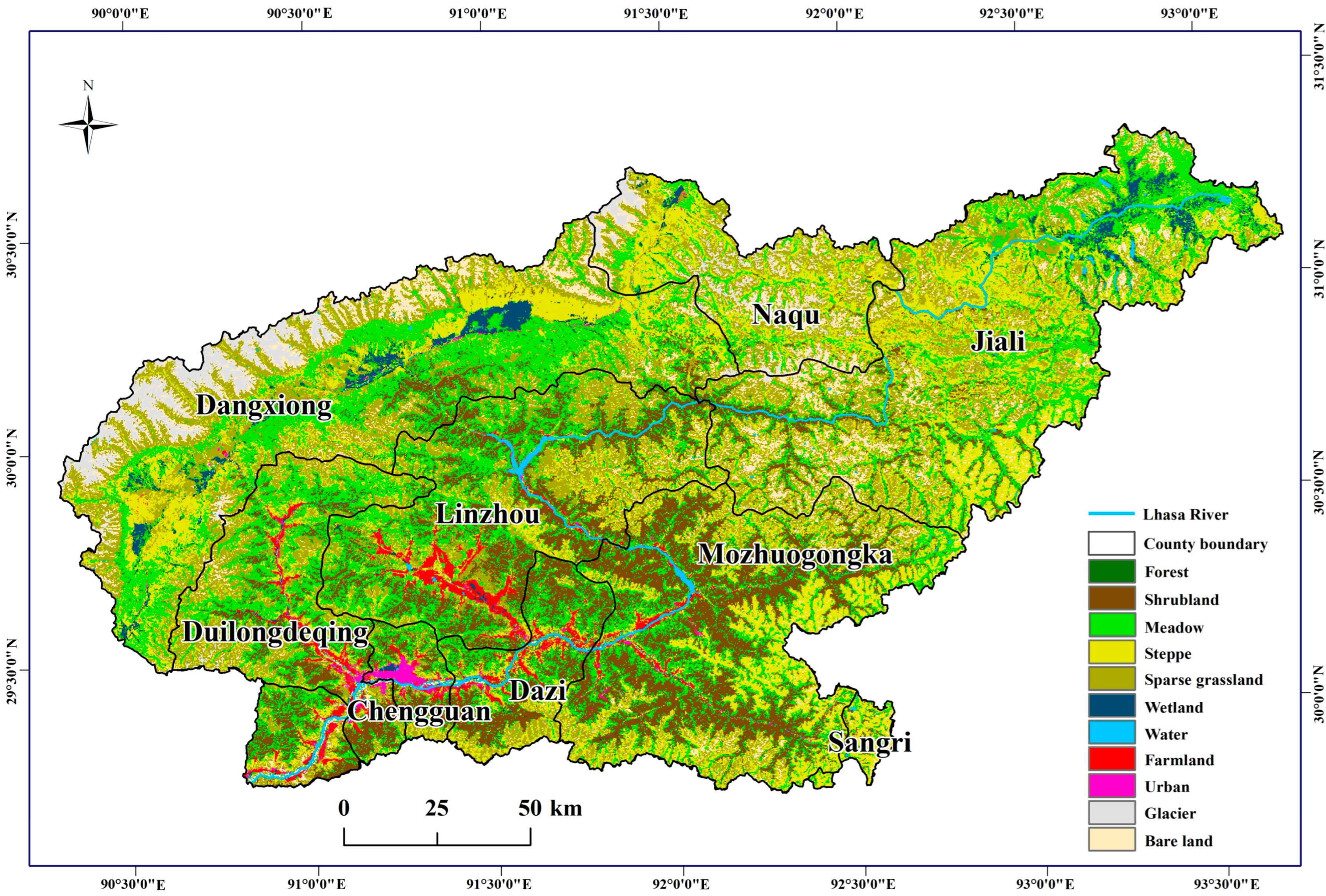
2.1. Study Area

The Lhasa River basin (90°05′–93°20′ E, 29°20′–31°15′ N) is located in the southern part of the Tibet Autonomous Region (Figure 1). The basin encompasses 10 districts and counties, including Chengguan District of Lhasa City and the surrounding areas, covering a total area of 3.26 × 10⁴ km². The average elevation of the Lhasa River basin is about 4500 m, the average annual temperature is from −7.1 to 9.2 °C, the average annual precipitation is from 340 to 700 mm, and approximately 90% of the precipitation is concentrated in June, July, and September [29]. The main ecosystem types are alpine meadows, wetlands, and forests [30]. Different ecosystem types have a diversity of ecological environments and climatic conditions, and these climates influence the growth and distribution of vegetation, which in turn affects ecosystem services such as soil conservation and the stable provision of water resources. These ecosystems provide local populations with numerous important ecosystem services, such as water conservation, soil conservation, and carbon sequestration. The population and economic development of the Tibet Autonomous Region are concentrated in the Lhasa River basin, where the rapid development of human activities has put pressure on the local ecological environment [26].

2.2. Data Sources and Descriptions

The data used in this study include land use type, digital elevation model (DEM), soil condition, meteorological condition, evapotranspiration, and socio-economic data (

Table 1. Description of data and data sources in this study.

Data	Resolution	Time Period
Land use data	250 m	2000, 2010, 2018
Ecosystem type data	90 m	2015
Digital elevation model (DEM)	30 m	2009
Soil map and attribute data	1 km	2012
Meteorological data (temperature and precipitation)	1 km	1980–2018
Evapotranspiration data	500 m	2000–2018
Social and economic data	1 km	2000, 2010, 2018

). Among them, land use data were obtained from the Resource and Environmental Science and Data Centre of the Chinese Academy of Sciences (RESDC-CAS) (http://www.resdc.cn, accessed on 11 November 2023) for 2000, 2010, and 2018, with a resolution of 250 m. Ecosystem type data were obtained from the China Ecosystem Assessment and Ecological Security Database (http://www.ecosystem.csdb.cn, accessed on 11 November 2023). DEM data were obtained from the Geospatial Data Cloud site, Computer Network Information Center, Chinese Academy of Sciences (http://www.gscloud.cn, accessed on 11 November 2023), with a resolution of 30 m. Soil data were obtained from the Harmonized World Soil Database supplied by the International Institute for Applied Systems Analysis and the Food and Agriculture Organization (http://webarchive.iiasa.ac.at, accessed on 11 November 2023). Temperature, precipitation, and other meteorological data were obtained from the China Meteorological Administration (http://www.cma.gov.cn, accessed on 11 November 2023). Spatial meteorological data were interpolated using the ANUSPLIN method. The evapotranspiration data from the MOD16A2 dataset were supplied by the USGS (https://lpdaac.usgs.gov, accessed on 11 November 2023). Socio-economic data mainly contain population and economic statistics, obtained from the Statistical Yearbooks (2000–2018) of Tibet.

2.3. Quantification of Ecosystem Services Supply

Based on the ecological characteristics of the Lhasa River basin and previous research [31,32], we selected four key ecosystem service supply (ESS) types, including carbon sequestration, habitat quality, water conservation, and soil conservation, as the supply in the coordination of ecosystem service supply and demand for quantitative assessment. The assessment was conducted on the time scale of 2000–2018. The Integrated Valuation of Ecosystem Services and Tradeoffs (InVEST v.3.6.0) model was used to assess ESS [26,33,34]. Carbon sequestration was measured by aboveground biomass, belowground biomass, soil, and dead organic matter. The calculation of habitat quality considered the degree of threats and the relative sensitivity of ecological stressors. Water conservation was based on the Budyko equation and annual average precipitation and calculated by the amount of water that is available as runoff within a watershed. Soil conservation was calculated by applying a modified generic soil loss equation. The detailed methods and parameters for quantifying ecosystem services are listed in Table S1.

2.4. Quantification of Ecosystem Services Demand

The demand for water supply services is derived from the actual per capita demand for water [35]. The demand for carbon sequestration arises from the carbon emissions generated through energy consumption during economic activities [36]. Habitat quality emphasizes the interdependent and shared relationship between humans and nature [37,38]. The extent of pressure exerted on the ecological environment by human activities affects the quantification of human demand for habitat quality. Considering that the demand for ecosystem services mainly originates from human societal needs, we chose three typical indicators (the land use development degree, the population density, and the GDP per km²) to reflect the ecosystem service demand [16,39,40,41]. Among them, the degree of land use intensity was calculated by the ratio of built-up land to total area, serving as an index of societal consumption intensity. The population density was directly related to ecosystem demand, with demand primarily varying due to changes in population size. The higher the population density, the higher the demand. GDP per km² represents the economic density and level of economic development in a region. As an economic indicator, it can reflect the overall demand of humans for goods and services, thus indirectly indicating the demand for ecosystem services by the people in the region.

The Lhasa River basin is located on the Qinghai–Tibet Plateau, and human activities are dominated by agricultural and pastoral production activities. Considering the regional natural environmental characteristics and data availability [22], the social demand for ESs can be quantified using the following equation:

$${ESD}_i=D_i\times \mathit{lg}\left({POP}_i+1\right)\times \mathit{lg}\left({GDP}_i+1\right)$$

(1)

where ${ESD}_i$ is the ES social demand of grid i; $D_i$, ${POP}_i$ and ${GDP}_i$ are the land use development degree, the population density, and the GDP per km² of grid i, respectively.

Compared to the other three categories of ecosystem services, the demand for soil conservation services is difficult to quantify using population density-related indicators due to the influence of factors such as topography, precipitation, and vegetation [35]. Using the sediment retention module of InVEST model, the soil conservation service demand was estimated by the revised universal soil loss equation (RUSLE).

ESDSC = R × K × LS × C × P

(2)

where ESDSC is the soil retention demand (t/(ha·yr)); R refers to rainfall erosivity (MJ mm hm⁻² h⁻¹ yr⁻¹); K refers to soil erodibility (t hm² h hm⁻² MJ⁻¹ mm⁻¹); LS refers to slope length and slope steepness; C refers to vegetation cover factor; and P refers to soil retention practice factor.

2.5. Supply–Demand Ratio of Ecosystem Service

Based on the ESS and ESD values, the min–max method was used to standardize the values of supply and demand for each ecosystem service to uniform values between 0 and 1. We utilize the ES supply and demand ratio (ESDR) to connect the actual supply values of ecosystem services with actual human demand, to characterize the relationship between ES supply and demand [6]. The formula is as follows:

$$ESDR=\frac{S-D}{(S_{max}+D_{max})/2}$$

(3)

S and D represent the normalized supply and demand of ecosystem services; $S_{max}$ is the maximum value of ES supply; and $D_{max}$ is the maximum value of ES demand. ESDR > 0 indicates that supply and demand are in a surplus state, ESDR = 0 indicates that supply and demand are in an equilibrium state, and ESDR < 0 indicates that supply and demand are in a deficit state.

2.6. Coupling Coordination Degree Model

Coupling, originating from physics, refers to the phenomenon in which two or more systems interact with each other and mutually influence one another [42]. According to the coupled coordination degree model, we can explore and match the spatiotemporal relationship between the supply and demand of ESs in the Lhasa River basin. We constructed the model using the following equations:

$$CC{D}_i=\sqrt{C_i\times T_i}$$

(4)

$$C_i=2\times \sqrt{\frac{x_{s_i}\times x_{D_i}}{{\left(x_{s_i}+x_{D_i}\right)}^2}}$$

(5)

$$T_i=\alpha \times x_{s_i}+\beta \times x_{D_i}$$

(6)

where $x_{s_i}$ and $x_{D_i}$ denote ES supply and ES demand, respectively, and $CC{D}_i$ is the coupling coordination degree of the supply and demand of ESs; the value of $CC{D}_i$ is between 0 and 1. The closer the coupling coordination degree is to 1, the higher the coupling coordination degree between ES supply and demand. $C_i$ represents the coupling degree of grid i, indicating the degree to which ES supply and demand interact with each other. $T_i$ refers to the coordination level, reflecting the overall synergy effect of ES supply and demand. Considering that the supply and demand of ESs are equally important as ecological, environmental, and human well-being for sustainable development in society, the same weight was taken as α = β = 0.5. To clearly show the difference in the ES supply and demand ratio (ESDR) level of coupling coordination, referring to previous studies and the actual situation in the Lhasa River basin, the CCD was divided into five levels [35,43,44]: lowest coupling coordination, low coupling coordination, moderate coupling coordination, high coupling coordination, and extremely high coupling coordination (

Table 2. The classification standard of the coupling coordination degree.

Range of CCD Values	Type	Range of CCD Values
0 ≤ CCD ≤ 0.1	Lowest coupling coordination	0 ≤ CCD ≤ 0.1
0.1 < CCD < 0.2	Low coupling coordination	0.1 < CCD < 0.2
0.2 < CCD < 0.5	Moderate coupling coordination	0.2 < CCD < 0.5
0.5 < CCD < 0.8	High coupling coordination	0.5 < CCD < 0.8
0.8 < CCD < 1	Extremely high coupling coordination	0.8 < CCD < 1

).

2.7. Spatial Autocorrelation Analysis

Spatial autocorrelation refers to the mutual correlation or interdependence between geographical phenomena or variables in geographic space. It reflects the distribution pattern and level of mutual influence of geographical phenomena in space [45]. By referring to previous research [6,10,45,46], global and local Moran’s I was applied to examine the global autocorrelation as well as the local spatial autocorrelation of CCD. The formula is as follows:

$$I=\frac{n}{S_0}\times \frac{\sum _{i=1}^n\sum _{j=1}^n{w}_{ij}\left(y_i-\bar{y}\right)\left(y_j-\bar{y}\right)}{\sum _{i=1}^n{\left(y_i-\bar{y}\right)}^2}$$

(7)

$$I_i=\frac{1}{n}\times \frac{\left(y_i-\bar{y}\right)\sum _{j=1}^n{w}_{ij}\left(y_i-\bar{y}\right)}{\sum _{i=1}^n{\left(y_i-\bar{y}\right)}^2}$$

(8)

where I is the global Moran’s I index for coordination degree; $I_i$ is the local Moran’s I index for the coordination degree; S₀ = $\sum _{i=1}^n\sum _{j=1}^n{w}_{ij}$; n represents the spatial unit number; $y_i$ and $y_j$ represent the attribute values of spatial unit i and spatial unit j, respectively; $\overline{y}$ is the average value of all spatial unit attributes; and $w_{ij}$ represents the spatial weight matrix for measuring the spatial correlation between the spatial units i and j.

Global and local Moran’s I index were calculated by using GeoDa (v.1.22) software. We used the zonal statistics tool in ArcGIS (v.10.8) to extract the average values of coupling coordination from township vector data within the Lhasa River basin. The K-nearest neighbor method was selected to compute spatial distance weights. The spatial agglomeration map was categorized into five types: not significant, high–high, low–low, low–high, and high–low. The range of Moran’s I is from −1 to 1, where positive values indicate a spatial positive correlation. The larger the value, the stronger the spatial correlation. Moran’s I < 0 indicates a negative correlation, with smaller values indicating greater spatial heterogeneity. Moran’s I = 0 indicates spatial randomness. We conducted Monte Carlo simulation tests to analyze the statistical significance of Moran’s I (random simulation times = 9999) and determined statistically significant values at the 0.1% level, which is considered credible evidence for the spatial correlation of CCD.

3. Results

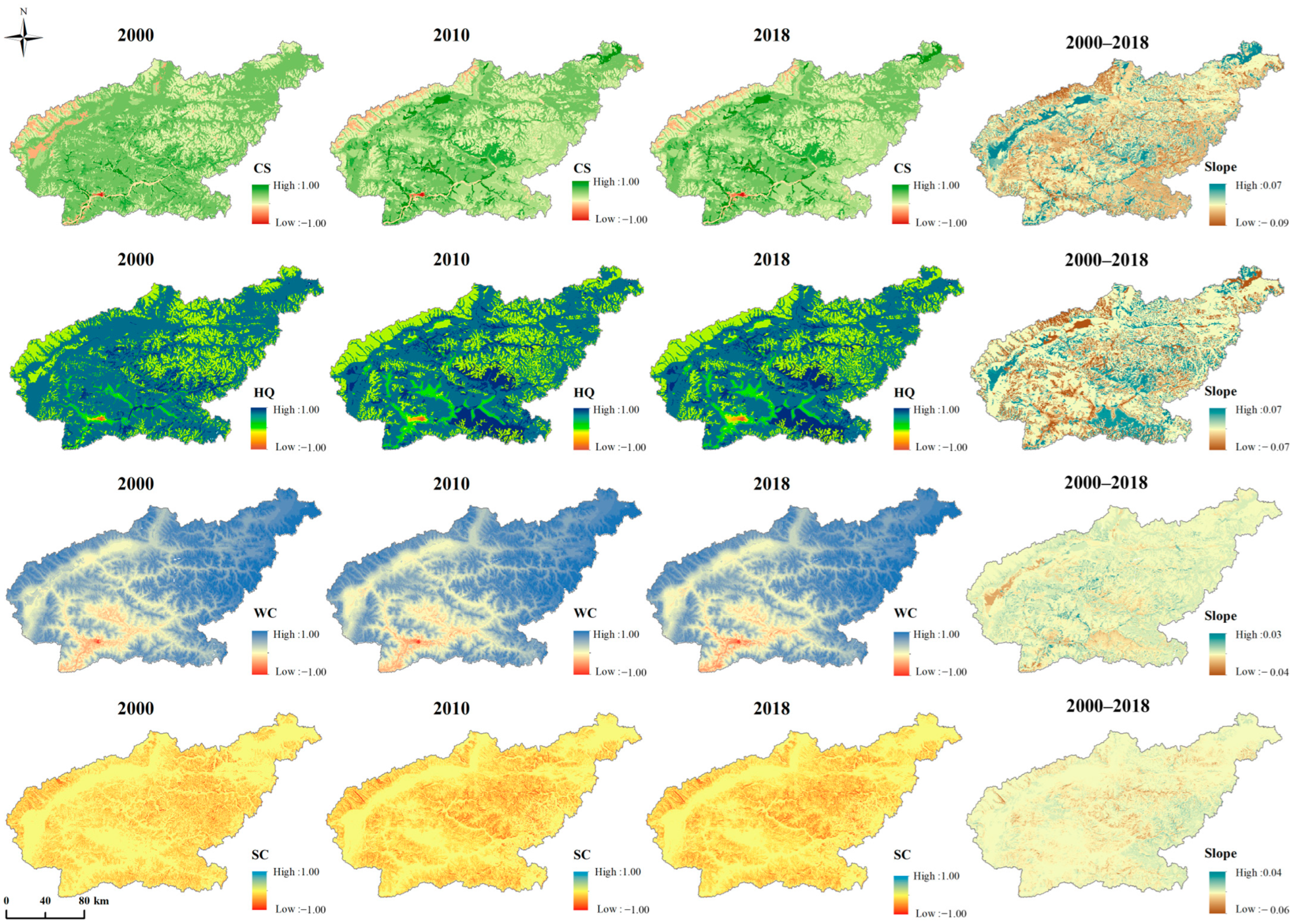
3.1. Spatial and Temporal Pattern of Ecosystem Service Supply and Demand

By calculating the ES supply and demand ratio (ESDR) of four selected ecosystem services (Figure 2), we analyzed the ecosystem service supply–demand matching status in the Lhasa River basin. The results indicated that there was significant spatial heterogeneity in the distribution of ESDRs. The main regions where carbon sequestration services were in negative ESDRs were the western part of Dangxiong County and Chengguan District, with the major ecosystem types being glaciers and urban land. ESDRs were higher in areas of cultivated land and grassland, such as the central part of Linzhou County and the northern part of Mozhugongka County. The ESDR of carbon sequestration services in Jiali County was close to 0, and the supply and demand were basically balanced. From 2000 to 2018, the mismatch between the supply and demand of carbon sequestration services in Chengguan District intensified, and the area with an ESDR of less than −0.5 increased by 71.65%. Areas where habitat quality has a supply–demand imbalance are mainly concentrated in the urban areas of Chengguan District. ESDR values in the remaining areas are all close to or greater than 0, indicating a state of balanced supply and demand. From 2000 to 2010, Chengguan District experienced a more severe imbalance in habitat quality supply and demand. The ESDR showed a declining trend, with the area of regions with negative ESDRs increasing by 50.20%. From 2010 to 2018, although the ESDR continued to decline, the rate of decline slowed down. The area of regions facing supply–demand imbalances increased by 72.17% compared to the year 2000. Regions with high ESDRs for water conservation services are primarily located in Jiali County and Naqu County in the upper reaches of the Lhasa River, while areas with supply–demand imbalances are mainly concentrated in the southwest part of the basin. Centered around Chengguan District, the ESDR for water conservation services exhibits a decreasing trend towards both southwest and northeast directions. The area where the ESDR was below −0.1 increased by 29.53% from 2000 to 2018. The ESDR of soil conservation services is generally insufficient throughout the entire region, with regions where the ESDR is lower than −0.1 mainly distributed in the central part of Jiali County, Naqu County, and the western part of Dangxiong County. The distribution is relatively scattered. From 2000 to 2010, there was a significant decline in the ESDR of soil conservation services. From 2010 to 2018, the ratio continued to decline, but at a slower rate. The area facing supply–demand imbalances increased by 56.61%.

The values of ESDR were extracted from four ecosystem services based on different ecosystem types (Figure 3). In terms of the total amount of carbon sequestration services, grasslands, being the largest ecosystem type in the Lhasa River basin, with their extensive vegetation cover and short growth cycles, contributed a rich organic carbon pool and continuously provided positive ESDR values from 2000 to 2018. For habitat quality, grasslands and forests with diverse vegetation cover contributed over 90% of positive ESDR values from 2000 to 2018, maintaining a good state where supply exceeded demand. Other ecosystem types and glaciers maintained a supply–demand balance. Before 2010, forests contributed the most to the excess supply, exceeding 30%, while water bodies surpassed forests as the largest contributor afterwards. From 2000 to 2018, the increasing demand for living environments due to population growth continued to rise, while urban areas had limited resource capacities. As a result, the habitat quality in urban areas was consistently unable to meet the demand. For water conservation services, grasslands continued to provide the highest and positive ESDRs, maintaining a share of 50% or more from 2000 to 2018.

In terms of per-unit area proportion, for carbon sequestration services, except for urban areas where there is a supply–demand imbalance, all other ecosystem types exhibit supply exceeding demand. As croplands are ecosystem types with high biomass, they have the highest proportion of ESDR per unit area, exceeding 30%. Glacial regions with low temperatures and rare vegetation cover have a minor impact on the supply–demand balance for carbon sequestration services, with ESDR values approaching 0. For habitat quality, between the years 2000 and 2018, grasslands and forests both contributed positive ESDR values of more than 90%, indicating a state where supply surpassed demand. Forests and grasslands usually have high biodiversity and vegetation cover, capable of providing high-quality habitats. Regarding the water conservation service, almost all ecosystem types provide positive ESDR with supply exceeding demand. Among them, urban areas with low surface permeability and disturbances in the water cycle have the lowest proportion. Compared with the three other types of ESs, in the statistical analysis of the soil conservation service, almost all ecosystem types provided negative ESDR values when considering both total quantity and per unit area. In terms of total quantity, grasslands contributed the largest share of negative ESDR values, exceeding 40%. As the largest ecosystem type in the Lhasa River basin, grasslands also serve as grazing areas for local herders. Continuous grazing leads to a decrease in grassland coverage, resulting in a situation where supply cannot meet demand.

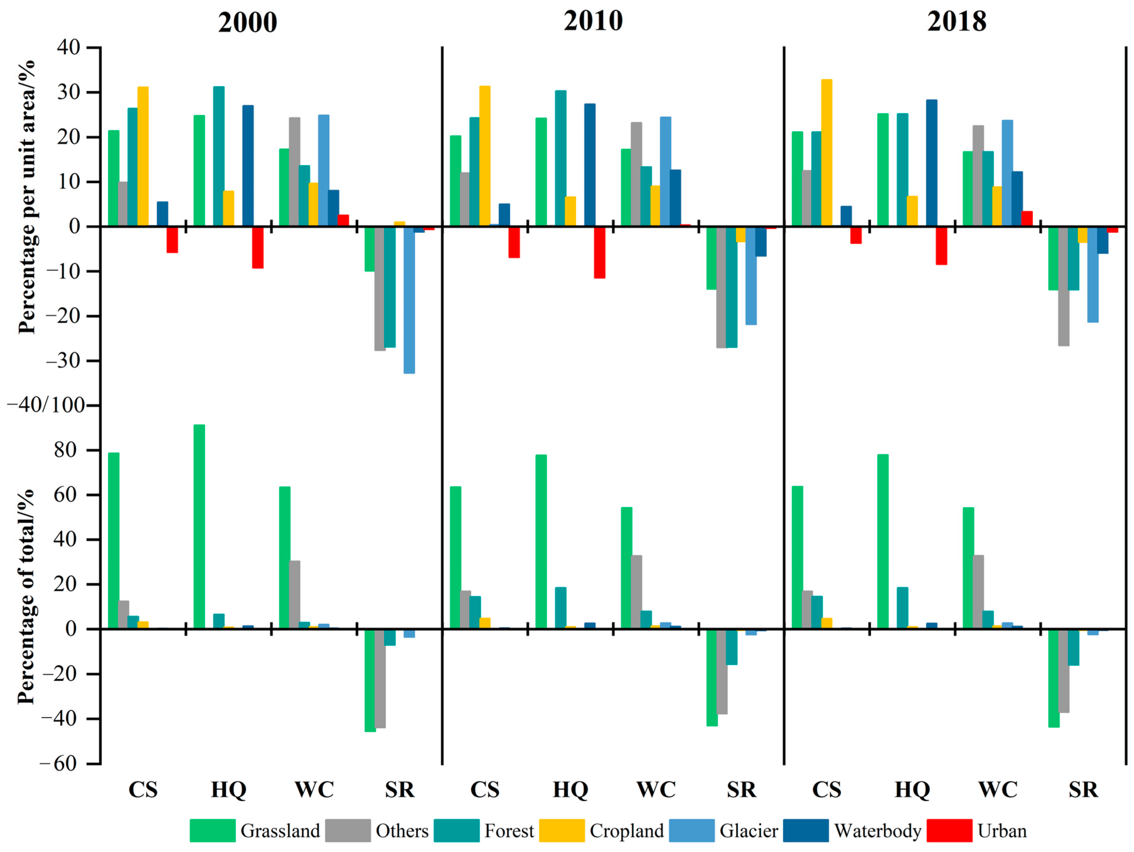
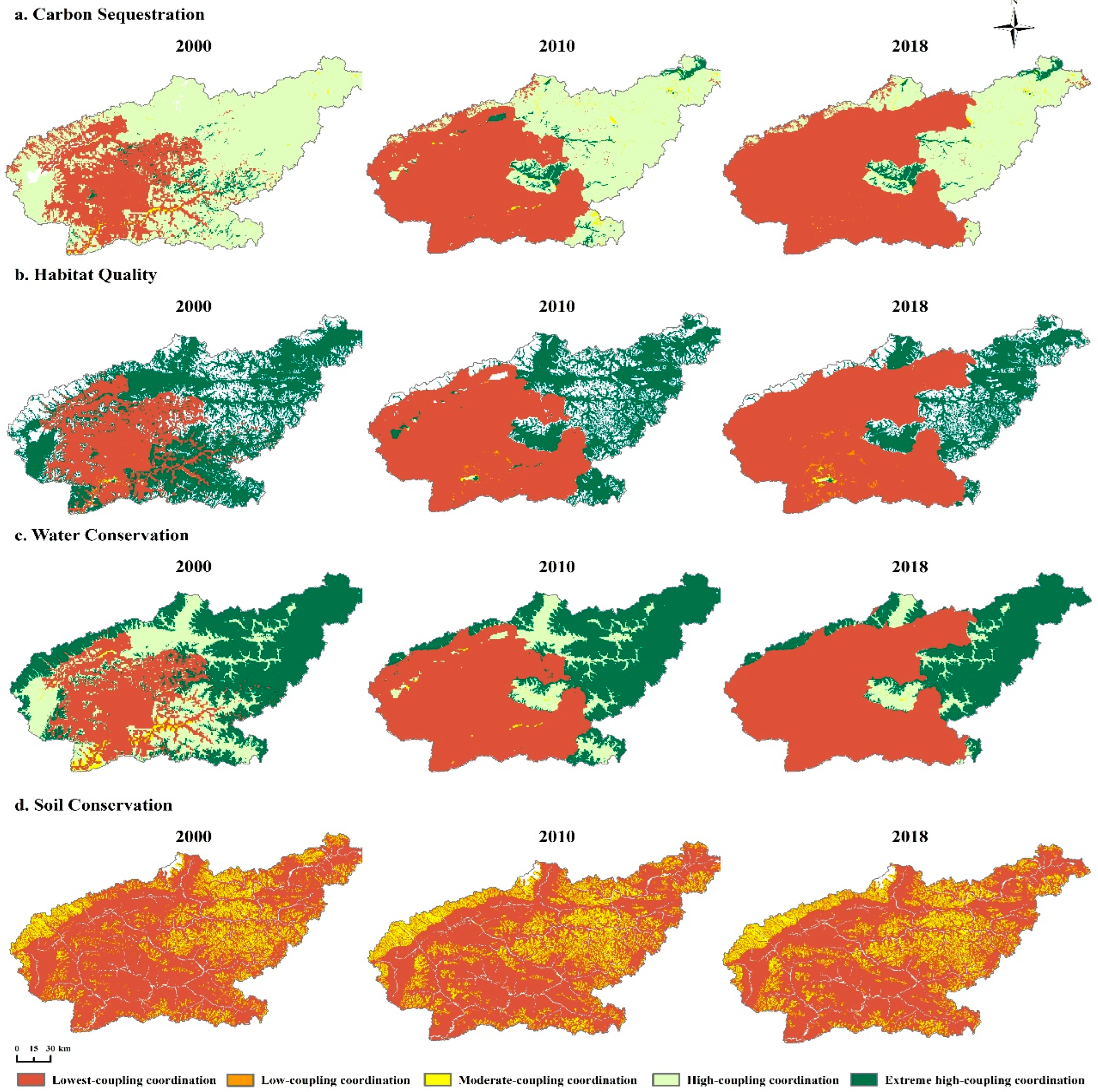
3.2. Coordination Pattern and Evolution Features of the Supply and Demand Coupling of Ecosystem Services

From Figure 4, we can explore the coupling coordination degree (CCD) between the supply and demand of ecosystem services of the Lhasa River from 2000 to 2018. Overall, the imbalance between supply and demand for carbon sequestration services significantly intensified from 2000 to 2018, with noticeable differences between them. Regions with the lowest coupling coordination and low coupling coordination, centered around Linzhou County, spread outward (Figure 4a) until the easternmost part of Nagqu County. From 2000 to 2018, the area proportion of the lowest coupling coordination increased from 30.5% to 64.4%. The remaining areas are classified as regions with high coupling coordination and extremely high coupling coordination. The distribution characteristics of CCD for habitat quality services are consistent with those of carbon sequestration services, but small-scale areas of high coupling and extremely high coupling types appear in the Chengguan area. After 2010, there were scattered areas of low coupling coordination and moderate coupling coordination near the Chengguan area (Figure 4b). The area of regions with the lowest coupling coordination gradually expanded upstream. By 2018, the proportion of areas with the lowest coupling coordination had reached 71.8%, an increase of 38.5% compared to 2000. The CCD for water conservation services exhibits characteristics consistent with those of carbon sequestration services, showing significant spatial heterogeneity. Apart from the regions with extremely low coupling coordination and low coupling coordination, the proportion of regions with extremely high coupling coordination for water conservation services is much larger than that of regions with high coupling coordination (Figure 4c). The area proportion of the lowest coupling coordination for water conservation services is the lowest among the four types of ESs, but by 2018, the proportion still reached 63.2%. In terms of soil conservation services, regions with extremely low coupling coordination dominate. Except for unused land and glaciers, which belong to moderate-coupling-coordination areas, all other regions exhibit extremely low coupling coordination (Figure 4d). The low-coupling-coordination areas are distributed along rivers in areas with high rainfall erosivity and high vegetation cover. From 2000 to 2018, the area proportion of regions with the lowest coupling coordination consistently remained around 75%.

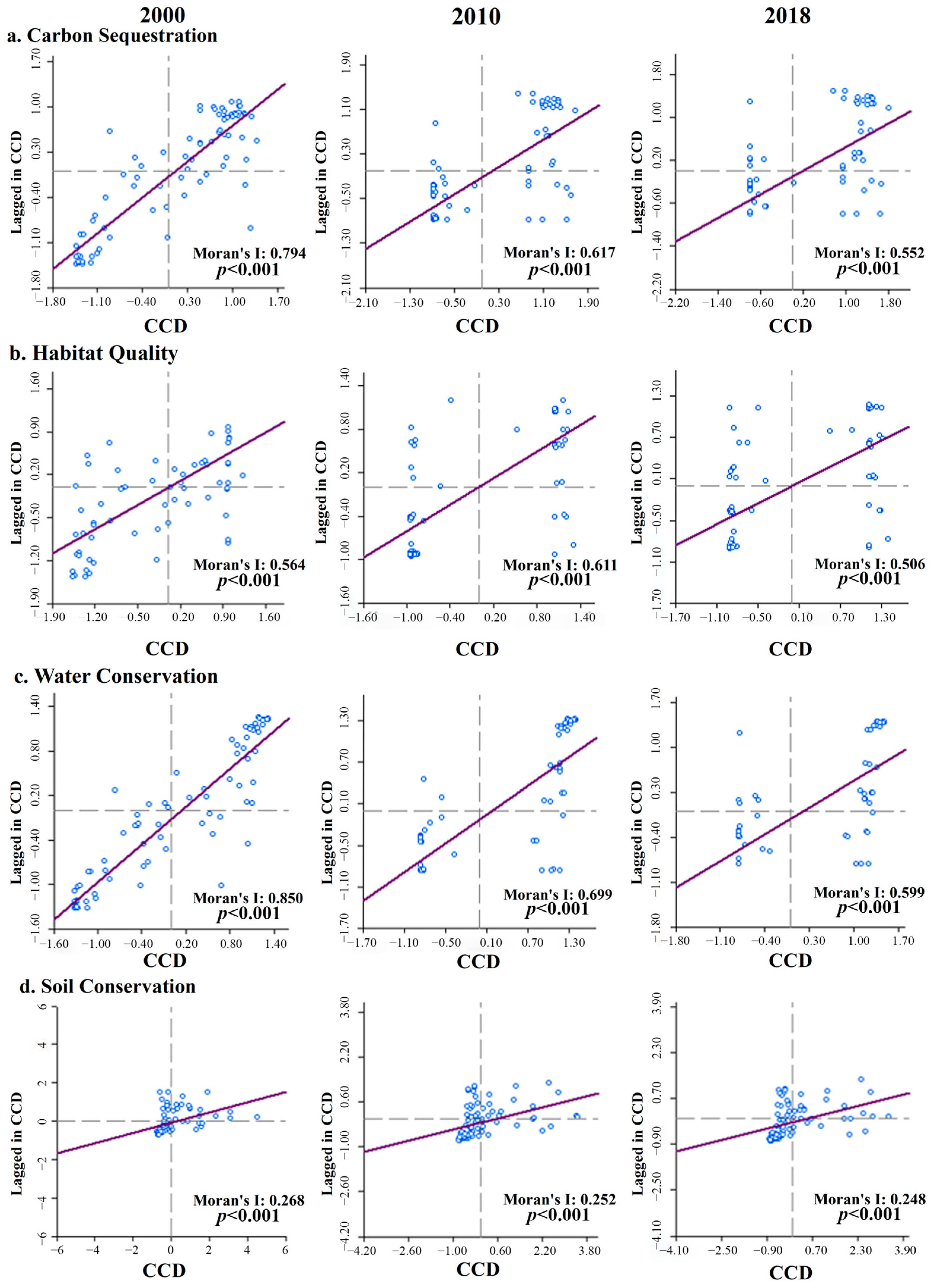
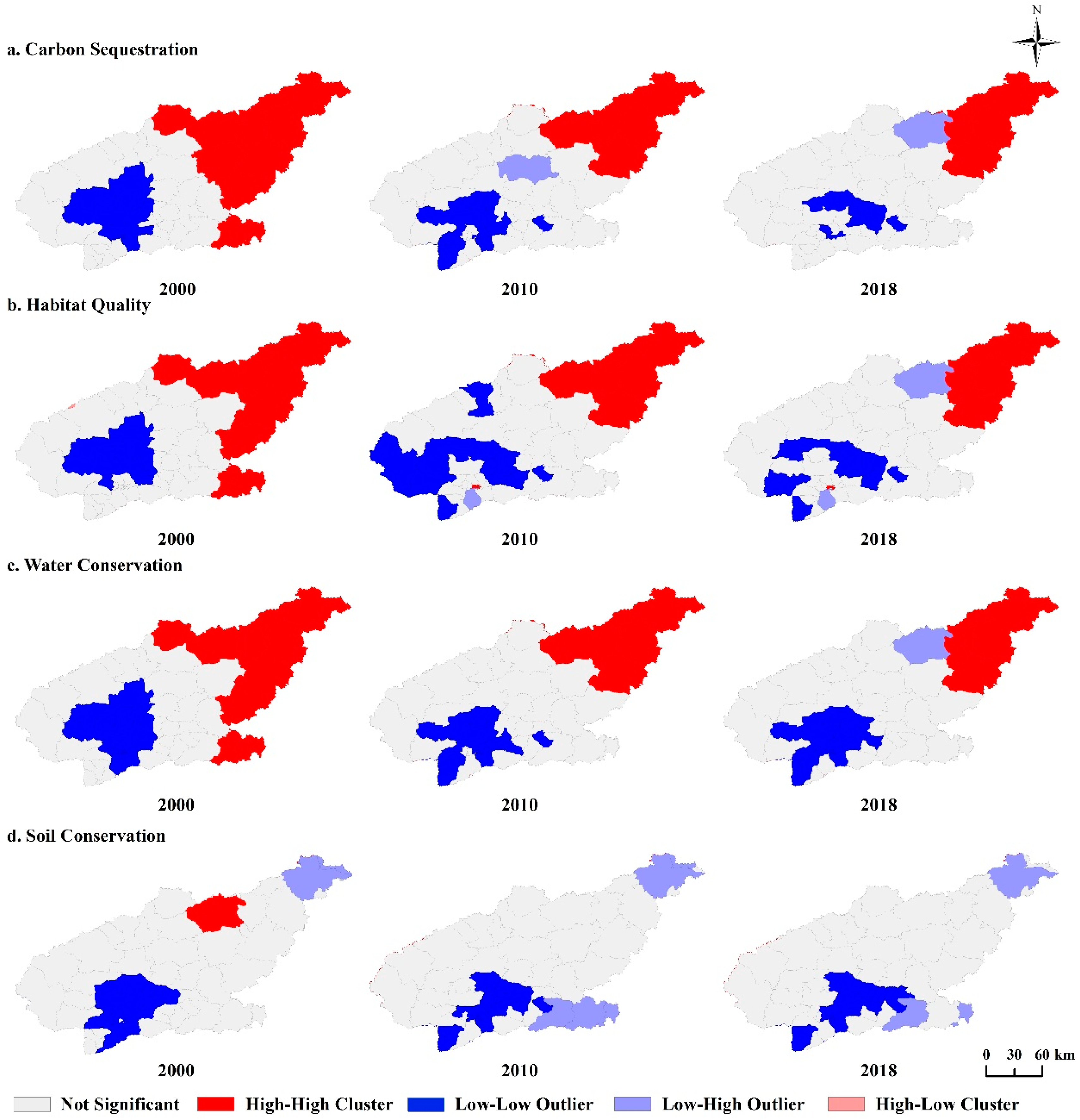
3.3. Spatial Autocorrelation of Ecosystem Service Supply–Demand Pattern

The global spatial correlation and changes in coupling coordination for various ecosystem services are shown in Figure 5. The Moran’s I indexes for carbon sequestration, habitat quality, and water conservation services are all above 0.5, while the Moran’s I index for soil conservation services is above 0.2. All measurements passed a 99% significance test. The positive values of Moran’s I indicate a significant spatial positive correlation between the supply and demand of ecosystem services in the Lhasa River basin. From 2000 to 2018, there were significant changes in Moran’s I index, with the largest change observed in carbon sequestration services and the smallest change in soil conservation services, both showing a decreasing trend. This suggests that the spatial correlation of coupling coordination between supply and demand for ecosystem services weakened over time, but overall still exhibits significant spatial clustering.

To further explore the spatiotemporal characteristics of supply–demand balance for ecosystem services in the Lhasa River basin, we conducted local spatial autocorrelation analysis. As shown in Figure 6, there is significant spatial heterogeneity in the coordination of supply and demand for ecosystem services in the Lhasa River basin, with notable changes in spatial distribution patterns. The study area is mainly characterized by four types of clustering: low–low (L-L), low–high (L-H), high–high (H-H), and non-significant aggregation. For carbon sequestration services, the high–high aggregation areas of supply–demand coordination are gradually shifting from the eastern part to the northeast. From 2000 to 2018, the number of H-H aggregation areas decreased from 23 to 14, with low–high areas emerging in the surrounding regions. The number of L-L aggregation areas decreased by 3, shifting from significant clustering to a more dispersed trend. In the distribution of supply–demand coordination for habitat quality services, the H-H aggregation areas in the eastern part show consistency with carbon sequestration services. However, after 2010, extremely small H-H aggregation areas emerged in the Chengguan District, with L-L aggregation areas dispersed in the surroundings. This indicates significant spatial heterogeneity in the supply–demand relationship for habitat quality services. For water conservation services, the H-H aggregation areas are situated in the northeast, while the L-L aggregation areas are located in the central region. From 2000 to 2018, the number of H-H aggregation areas continuously decreased, with low aggregation areas appearing in the peripheral regions. The supply–demand relationship for water conservation services deteriorated, as the number of L-L aggregation areas increased from 26 to 29, with the distribution gradually spreading towards the southern part. The number of H-H aggregation areas for soil conservation services decreased to 0 after 2000, with L-L aggregation areas becoming predominant. In the northeast and southeast, there were a few L-H aggregation areas, with both increasing by 2 in number. This indicates that while there was a significant spatial correlation for soil conservation services, the supply–demand coordination relationship was poor. The number of areas with low coordination is continuously increasing.

4. Discussion

4.1. Dynamic Analysis of Supply–Demand Coupling of Ecosystem Services

In the Lhasa River basin, grassland and forest are the main types of ecosystems, while the urban area is mainly concentrated in the densely populated Chengguan District. According to the results of the ES supply and demand ratio (ESDR), low values of the ESDR in the Lhasa River basin are concentrated in the southern Chengguan District and its surrounding areas. In terms of the contribution of per-unit area ecosystem types to the ESDR, the ESDR of the urban area is significantly and continuously negative. Due to the continuous increase in urban population and economic development, cities require a large amount of water resources to meet the needs of residents and industries. At the same time, they also need a significant amount of energy to support the operation of the city, resulting in a high demand for ESs such as water production and carbon sequestration in this region. However, this high-demand pattern imposes a certain burden on the ecosystem. Between 2000 and 2018, the area of low-ESDR regions continued to expand outward from the Chengguan District. This is consistent with the research results of [28], indicating a relative scarcity of actual ecological resources compared to demand during the process of regional economic development. ESDR values are generally higher in ecosystems such as grassland and forest, showing a good trend of supply exceeding demand. However, from the perspective of coupled coordination analysis, regions where supply exceeds demand do not necessarily exhibit good coordination. For example, the Yangbajing basin, as an important pastoral area in the Lhasa River basin, experiences relatively low environmental pressure from population and economic development, resulting in a positive ESDR, yet it still falls under the category of lowest coupling coordination. Therefore, when considering the mismatch in supply and demand of ESs in the Lhasa River basin, we classify the situations into two major categories: (1) large demand and small supply, indicating that demand exceeds supply; (2) large supply and small demand, indicating a lack of coordination between supply and demand. Although the Yangbajing basin has a surplus of supply over demand, the lack of coordination in ES supply and demand is still evident when demand is low. Therefore, in addition to the under-supply of ESs in areas with high population and urban agglomeration, regions predominantly consisting of forest and grassland ecosystems exhibit a mismatch between the supply and demand of ESs, resulting in a lower spatial–temporal distribution pattern of ES coupling coordination in the Lhasa River basin. When addressing the issue of supply–demand mismatch, it is crucial to consider the specific conditions of each region and not merely focus on increasing supply or demand in isolation. Based on the results of different types of coupling coordination, identifying and resolving supply–demand imbalances in different regions is key to achieving sustainable development in the Lhasa River basin.

According to spatial autocorrelation analysis, there is a certain degree of spatial heterogeneity in the coupling coordination among different regions of the Lhasa River. The headwater region of the Lhasa River and the downstream urban cluster region are both significantly influenced by their surrounding areas, showing significant agglomeration. The upstream region of the Lhasa River basin exhibits a clustered distribution with an H-H coupling coordination. Taking Jiali County as an example, with natural grasslands and forests as the predominant vegetation types, it is relatively less affected by population and economic activities. The ecosystem remains relatively intact, thus providing an ample supply of ESs, serving as a typical ecological “output” area in the region [28]. While the urban cluster areas in the southern part of the Lhasa River basin are constrained by limited resource supply, the high population density and economic activities result in a high demand for ESs [47], leading to a relatively insufficient supply and an L-L clustering distribution of coupling coordination. We can utilize the spatial autocorrelation relationship of this L-L coupling coordination for spatial propagation and interaction to effectively formulate ecosystem conservation and restoration strategies within the region.

4.2. Implications of Ecosystem Services Supply–Demand Contradiction

The research findings indicate that areas of supply–demand mismatch mainly occur in the central and western regions of the Lhasa River basin, where eight counties, including Chengguan District and Damxung County, exhibit the lowest coupling coordination. The downstream area of the Lhasa River is characterized by developed agriculture and the highest population density. Counties located downstream are experiencing urbanization, where the insufficient supply of ecosystem resources relative to the demands of urban development has led to a tense relationship between ecosystem service supply and urban growth. This imbalance has resulted in an increasing discord in the relationship between humans and the environment [48]. In addition to the high demand for ESs driven by local urban development, the tourism industry, as a key pillar of the local economy, has led to a concentration of tourist populations mainly in Chengguan District [49]. The significant demand for water resources brought by the tourism industry has exacerbated the serious supply–demand contradiction in water-provisioning services. Compared to other ESs, areas with low water-provisioning service ESDRs have a larger geographical coverage, with ecosystems predominantly characterized by urban areas and agricultural lands. The development of urbanization, tourism, and related industries has constrained the supply–demand coordination of ESs. It is essential to formulate relevant policies, optimize the structure of green economic development, enhance ecological environment protection, promote synchronized social, economic, and ecological development in the Lhasa River basin, and achieve the coordination of supply and demand for ESs. The coordination of supply and demand in the middle and upper reaches of the Lhasa River basin is relatively good, especially in the headwater region, where human activities have minimal disturbance and ESs remain intact. The area at the border between Linzhou County and Mozhuogongka County exhibits relatively high coupling coordination, located in the middle of the Lhasa River basin with forests as the predominant ecosystem type, showing a higher level of supply–demand coordination. However, other regions within Linzhou County and Mozhuogongka County face the lowest coupling coordination internally, leading to supply shortages relative to demand. Considering the differences in supply–demand coordination between regions, if the supply of certain ESs exceeds demand while the supply of other services fails to meet demand, effective allocation of ecological resources cannot be achieved [50], thereby affecting economic development and social well-being. When addressing the issue of supply–demand coordination of ESs in the Lhasa River basin, measures such as inter-regional cooperation and optimized resource allocation can be employed to resolve the imbalance between supply and demand. This approach can promote the coordination of supply and demand for ESs and contribute to sustainable development in the Lhasa River basin. Additionally, the government can implement rational land use planning to protect areas with high ES supply while optimizing the utilization of ES resources.

5. Conclusions

Based on dynamic spatial analysis of the supply and demand of the four types of ecosystem services (ESs) in the Lhasa River basin, this study reveals the matching status, coupling degree, and coordination of ESs. The main conclusions are as follows: (1) The mismatch between ES supply and demand of four types of ESs was concentrated in urban areas. The high demand in urban areas is one of the main reasons for the imbalance in ES demand in the basin. (2) From 2000 to 2008, the coupling coordination patterns of ES supply and demand in the Lhasa River basin were mainly characterized by a lack of coordination, with most areas belonging to the lowest coupling coordination level. The low-coupling patterns included both under-supply and over-supply of ESs. (3) The spatial distribution of the coupling coordination degree of ESs in the Lhasa River basin exhibited significant spatial heterogeneity. The high–high aggregation areas were concentrated in the northeast of the Lhasa River basin, where human activities have less influence. Measures such as inter-regional cooperation and optimal allocation of resources should be taken based on the connections between different regions to address the issue of supply–demand imbalance. Research could benefit from datasets that are more temporally consistent and of higher resolution to account for the nuanced temporal and spatial variations in ES supply–demand dynamics, with a focus on more accurately depicting how ecological processes affect the provision of ecosystem services. Despite its limitations, this study provides guidance on the rational allocation and integration of ecological resources in ecologically vulnerable areas from the perspectives of ecosystem types, supply–demand matching, and coupling coordination, enhancing the sustainability of regional development.

References

1. Costanza, R.; d’Arge, R.; de Groot, R.; Farber, S.; Grasso, M.; Hannon, B.; Limburg, K.; Naeem, S.; O’Neill, R.V.; Paruelo, J.; et al. The value of the world’s ecosystem services and natural capital. Nature 1997, 387, 253–260. [Google Scholar] [CrossRef]
2. Ouyang, Z.; Zhu, C.; Yang, G.; Xu, W.; Zheng, H.; Zhang, Y.; Xiao, Y. Gross ecosystem product: Concept, accounting framework and case study. Acta Ecol. Sin. 2013, 33, 6747–6761. [Google Scholar] [CrossRef]
3. Arowolo, A.O.; Deng, X.; Olatunji, O.A.; Obayelu, A.E. Assessing Changes in the Value of Ecosystem Services in Response to Land-Use/Land-Cover Dynamics in Nigeria. Sci. Total Environ. 2018, 636, 597–609. [Google Scholar] [CrossRef] [PubMed]
4. Cerretelli, S.; Poggio, L.; Gimona, A.; Yakob, G.; Boke, S.; Habte, M.; Coull, M.; Peressotti, A.; Black, H. Spatial Assessment of Land Degradation through Key Ecosystem Services: The Role of Globally Available Data. Sci. Total Environ. 2018, 628–629, 539–555. [Google Scholar] [CrossRef] [PubMed]
5. Liu, H.; Xing, L.; Wang, C.; Zhang, H. Sustainability Assessment of Coupled Human and Natural Systems from the Perspective of the Supply and Demand of Ecosystem Services. Front. Earth Sci. 2022, 10, 1025787. [Google Scholar] [CrossRef]
6. Ming, L.; Chang, J.; Li, C.; Chen, Y.; Li, C. Spatial-Temporal Patterns of Ecosystem Services Supply-Demand and Influencing Factors: A Case Study of Resource-Based Cities in the Yellow River Basin, China. Int. J. Environ. Res. Public Health 2022, 19, 16100. [Google Scholar] [CrossRef] [PubMed]
7. Huang, C.; Zeng, J.; Chen, W.; Cui, X. Spatiotemporal Characteristics of the Coupled Coordination Degree of Ecosystem Services Supply and Demand in Chinese National Nature Reserves. Int. J. Environ. Res. Public Health 2023, 20, 4845. [Google Scholar] [CrossRef] [PubMed]
8. Zhang, X.; Liu, Y.; Wang, Y.; Yuan, X. Interactive Relationship and Zoning Management between County Urbanization and Ecosystem Services in the Loess Plateau. Ecol. Indic. 2023, 156, 111021. [Google Scholar] [CrossRef]
9. Zhao, W.; Liu, Y.; Daryanto, S.; Fu, B.; Wang, S.; Liu, Y. Metacoupling Supply and Demand for Soil Conservation Service. Curr. Opin. Environ. Sustain. 2018, 33, 136–141. [Google Scholar] [CrossRef]
10. Wang, X.; Jia, Z.; Feng, X.; Ma, J.; Zhang, X.; Zhou, J.; Fu, X. Analysis on supply and demand balance of soil conservation service and its driving factors on the Loess Plateau. Acta Ecol. Sin. 2023, 43, 2722–2733. [Google Scholar] [CrossRef]
11. Chen, X.; Li, F.; Li, X.; Hu, Y.; Hu, P. Evaluating and Mapping Water Supply and Demand for Sustainable Urban Ecosystem Management in Shenzhen, China. J. Clean. Prod. 2020, 251, 119754. [Google Scholar] [CrossRef]
12. Meng, S.; Huang, Q.; Zhang, L.; He, C.; Inostroza, L.; Bai, Y.; Yin, D. Matches and Mismatches between the Supply of and Demand for Cultural Ecosystem Services in Rapidly Urbanizing Watersheds: A Case Study in the Guanting Reservoir Basin, China. Ecosyst. Serv. 2020, 45, 101156. [Google Scholar] [CrossRef]
13. Yoshimura, N.; Hiura, T. Demand and Supply of Cultural Ecosystem Services: Use of Geotagged Photos to Map the Aesthetic Value of Landscapes in Hokkaido. Ecosyst. Serv. 2017, 24, 68–78. [Google Scholar] [CrossRef]
14. Li, F.; Sun, R.; Yang, L.; Chen, L. Assessment of fresh water ecosystem services in Beijing based on demand and supply. Chin. J. Appl. Ecol. 2010, 21, 1146–1152. [Google Scholar] [CrossRef]
15. Liu, G.; Zhang, L.; Zhang, Q. Spatial and temporal dynamics of land use and its influence on ecosystem service value in Yangtze River Delta. Acta Ecol. Sin. 2014, 34, 3311–3319. [Google Scholar]
16. Peng, J.; Yang, Y.; Xie, P.; Liu, Y. Zoning for the construction of green space ecological networks in Guangdong Province based on the supply and demand of ecosystem services. Acta Ecol. Sin. 2017, 37, 4562–4572. [Google Scholar]
17. Jing, Y.; Chen, L.; Sun, R. A theoretical research framework for ecological security pattern construction based on ecosystem services supply and demand. Acta Ecol. Sin. 2018, 38, 4121–4131. [Google Scholar]
18. Yang, D.; Zhu, C.; Li, J.; Li, Y.; Zhang, X.; Yang, C.; Chu, S. Exploring the Supply and Demand Imbalance of Carbon and Carbon-Related Ecosystem Services for Dual-carbon Goal Ecological Management in the Huaihe River Ecological Economic Belt. Sci. Total Environ. 2024, 912, 169169. [Google Scholar] [CrossRef]
19. Lu, H.; Stringer Lindsay, C.; Yan, Y.; Wang, C.; Zhao, C.; Rong, Y.; Zhu, J.; Wu, G.; Martin, D. Mapping ecosystem service supply and demand: Historical changes and projectionsunder SSP-RCP scenarios. Acta Ecol. Sin. 2023, 43, 1309–1325. [Google Scholar]
20. Zhang, P.; Zhu, X.; He, Q.; Ouyang, X. Spatial-temporal differentiation and balance pattern of supply and demand of ecosystem services of the Yangtze River Economic Zone. Ecol. Sci. 2020, 39, 155–166. [Google Scholar] [CrossRef]
21. Hou, L.; Wu, F.; Xie, X. The Spatial Characteristics and Relationships Between Landscape Pattern and Ecosystem Service Value along an Urban-Rural Gradient in Xi’an City, China. Ecol. Indic. 2020, 108, 105720. [Google Scholar] [CrossRef]
22. Xu, L.; Yang, D.; Liu, D.; Lin, H. Spatiotemporal Distribution Characteristics and Supply-Demand Relationships of Ecosystem Services on the Qinghai-Tibet Plateau, China. Mt. Res. 2020, 38, 483–494. [Google Scholar] [CrossRef]
23. Zheng, B.; Xu, Q.; Shen, Y. The Relationship Between Climate Change and Quaternary Glacial Cycles on the Qinghai-Tibetan Plateau: Review and Speculation. Quaternary 2002, 97–98, 93–101. [Google Scholar] [CrossRef]
24. Zhang, S.; Wu, T.; Guo, L.; Zhao, Y. Assessing Ecological Risk on the Qinghai-Tibet Plateau Based on Future Land Use Scenarios and Ecosystem Service Values. Ecol. Indic. 2023, 154, 110769. [Google Scholar] [CrossRef]
25. Shi, W.; Qiao, F.; Zhou, L. Identification of Ecological Risk Zoning on Qinghai-Tibet Plateau from the Perspective of Ecosystem Service Supply and Demand. Sustainability 2021, 13, 5366. [Google Scholar] [CrossRef]
26. Han, W.; Su, X.; Lu, H.; Li, T.; Jin, T.; Zhang, M.; Liu, G. Impacts of Human Activity Intensity on Ecosystem Services for Conservation in the Lhasa River Basin. Ecosyst. Health Sustain. 2023, 9, 0088. [Google Scholar] [CrossRef]
27. An, B.; Yao, T.; Guo, Y.; Wang, W.; Li, J.; Li, X.; Wang, Z. Protection, Restoration, and Governance Technology Demonstration System in the Typical Regions of the Lhasa River Basin. Chin. J. 2021, 66, 2775–2784. [Google Scholar] [CrossRef]
28. Huang, L.; He, C.; Wang, B. Study on the Spatial Changes Concerning Ecosystem Services Value in Lhasa River Basin, China. Environ. Sci. Pollut. Res. 2022, 29, 7827–7843. [Google Scholar] [CrossRef] [PubMed]
29. Shui, Y.; Lu, H.; Wang, F.; Yan, Y.; Wu, G. Assessment of habitat quality on the basis of land cover and NDVI changes in Lhasa River Basin. Acta Ecol. Sin. 2018, 38, 8946–8954. [Google Scholar]
30. Zhang, S.; Lei, Y.; Yao, Q.; Li, H. Runoff Response to Land Cover and Climate Change in Lhasa River Basin. Water Resour. Prot. 2010, 26, 39–44. [Google Scholar]
31. Lu, H.; Huang, Q.; Zhu, J.; Zheng, T.; Yan, Y.; Wu, G. Ecosystem Type and Quality Changes in Lhasa River Basin and Their Effects on Ecosystem Services. Acta Ecol. Sin. 2018, 38, 8911–8918. [Google Scholar]
32. Liang, Y.; Song, W. Integrating Potential Ecosystem Services Losses into Ecological Risk Assessment of Land Use Changes: A Case Study on the Qinghai-Tibet Plateau. J. Environ. Manag. 2022, 318, 115607. [Google Scholar] [CrossRef] [PubMed]
33. Ouyang, Z.; Zheng, H.; Xiao, Y.; Polasky, S.; Liu, J.; Xu, W.; Wang, Q.; Zhang, L.; Xiao, Y.; Rao, E.; et al. Improvements in Ecosystem Services from Investments in Natural Capital. Science 2016, 352, 1455–1459. [Google Scholar] [CrossRef] [PubMed]
34. Sharp, R.; Tallis, H.; Ricketts, T.; Guerry, A.; Wood, S.; Chaplin-Kramer, R.; Nelson, E.; Ennaanay, D.; Wolny, S.; Olwero, N. InVEST 3.6. 0 User’s Guide; Collaborative Publication by the Natural Capital Project, Stanford University, The University of Minnesota, The Nature Con-servancy, and World Wildlife Fund; Stanford University: Stanford, CA, USA, 2018. [Google Scholar]
35. Li, P.; Liu, C.; Liu, L.; Wang, W. Dynamic Analysis of Supply and Demand Coupling of Ecosystem Services in Loess Hilly Region: A Case Study of Lanzhou, China. Chin. Geogr. Sci. 2021, 31, 276–296. [Google Scholar] [CrossRef]
36. Liu, Y.; Zhao, M. Linking Ecosystem Service Supply and Demand to Landscape Ecological Risk for Adaptive Management: The Qinghai-Tibet Plateau Case. Ecol. Indic. 2023, 146, 109796. [Google Scholar] [CrossRef]
37. Burkhard, B.; Kroll, F.; Nedkov, S.; Müller, F. Mapping Ecosystem Service Supply, Demand and Budgets. Ecol. Indic. 2012, 21, 17–29. [Google Scholar] [CrossRef]
38. Wolff, S.; Schulp, C.J.E.; Verburg, P.H. Mapping Ecosystem Services Demand: A Review of Current Research and Future Perspectives. Ecol. Indic. 2015, 55, 159–171. [Google Scholar] [CrossRef]
39. Wang, C.; Wu, X.; Fu, B.; Han, X.; Chen, Y.; Wang, K.; Zhou, H.; Feng, X.; Li, Z. Ecological Restoration in the Key Ecologically Vulnerable Regions: Current Situation and Development Direction. Acta Ecol. Sin. 2019, 39, 7333–7343. [Google Scholar]
40. Liu, C.; Yang, M.; Hou, Y.; Xue, X. Ecosystem Service Multifunctionality Assessment and Coupling Coordination Analysis with Land Use and Land Cover Change in China’s Coastal Zones. Sci. Total Environ 2021, 797, 149033. [Google Scholar] [CrossRef]
41. Xu, Q.; Yang, R.; Zhuang, D.; Lu, Z. Spatial Gradient Differences of Ecosystem Services Supply and Demand in the Pearl River Delta Region. J. Clean. Prod. 2021, 279, 123849. [Google Scholar] [CrossRef]
42. Li, Y.; Li, Y.; Zhou, Y.; Shi, Y.; Zhu, X. Investigation of a Coupling Model of Coordination between Urbanization and the Environment. J. Environ. 2012, 98, 127–133. [Google Scholar] [CrossRef] [PubMed]
43. Yu, J.; Yi, L.; Xie, B.; Li, X.; Li, J.; Xiao, J.; Zhang, L. Matching and Coupling Coordination between the Supply and Demand for Ecosystem Services in Hunan Province, China. Ecol. Indic. 2023, 157, 111303. [Google Scholar] [CrossRef]
44. Zhang, S.; Wu, T.; Guo, L.; Zou, H.; Shi, Y. Integrating Ecosystem Services Supply and Demand on the Qinghai-Tibetan Plateau Using Scarcity Value Assessment. Ecol. Indic. 2023, 147, 109969. [Google Scholar] [CrossRef]
45. Naimi, B.; Hamm, N.A.S.; Groen, T.A.; Skidmore, A.K.; Toxopeus, A.G.; Alibakhshi, S. ELSA: Entropy-Based Local Indicator of Spatial Association. Spat. Stat. 2019, 29, 66–88. [Google Scholar] [CrossRef]
46. Anselin, L. Local Indicators of Spatial Association-LISA. Geogr. Anal. 1995, 27, 93–115. [Google Scholar] [CrossRef]
47. Lu, H.; Yan, Y.; Zhu, J.; Jin, T.; Liu, G.; Wu, G.; Stringer, L.C.; Dallimer, M. Spatiotemporal Water Yield Variations and Influencing Factors in the Lhasa River Basin, Tibetan Plateau. Water 2020, 12, 1498. [Google Scholar] [CrossRef]
48. Chen, T.; Jiao, J.; Chen, Y.; Lin, H.; Wang, H.; Bai, L. Distribution and Land Use Characteristics of Alluvial Fans in the Lhasa River Basin, Tibet. J. Geogr. Sci. 2021, 31, 1437–1452. [Google Scholar] [CrossRef]
49. Li, D.; Tian, P.; Shao, D.; Hu, T.; Luo, H.; Dong, B.; Khan, S.; Cui, Y.; Luo, Y. Assessment of Water Pollution in the Tibetan Plateau with Contributions from Agricultural and Economic Sectors: A Case Study of Lhasa River Basin. Environ. Sci. Pollut. Res. 2022, 29, 20617–20631. [Google Scholar] [CrossRef]
50. Wang, H.; Wang, L.; Fu, X.; Yang, Q.; Wu, G.; Guo, M.; Zhang, S.; Wu, D.; Zhu, Y.; Deng, H. Spatial-Temporal Pattern of Ecosystem Service Supply-Demand and Coordination in the Ulansuhai Basin, China. Ecol. Indic. 2022, 143, 109406. [Google Scholar] [CrossRef]
Figure 1. Location and ecosystem types of the Lhasa River basin [26].
Land 13 00510 g001
Figure 2. Spatial patterns of ESDRs in the Lhasa River basin. CS: carbon sequestration; HQ: habitat quality, WC: water conservation; SC: soil conservation.
Land 13 00510 g002
Figure 3. Contribution of different ecosystem types to ES supply and demand ratio (ESDR) in 2000, 2010, and 2018.
Land 13 00510 g003
Figure 4. The coupling coordination degree (CCD) between ES supply and demand in the Lhasa River basin.
Land 13 00510 g004
Figure 5. Moran’s I indexes for supply and demand of ES coupling coordination degree.
Land 13 00510 g005
Figure 6. Spatial correlations of supply and demand of ES coupling coordination degree (CCD).
Land 13 00510 g006