Article

Estimating the Soil Copper Content of Urban Land in a Megacity Using Piecewise Spectral Pretreatment

1
School of Public Administration, Guangdong University of Finance & Economics, Guangzhou 510320, China
2
State Key Laboratory of Subtropical Building and Urban Science & Guangdong–Hong Kong-Macau Joint Laboratory for Smart Cities & MNR Key Laboratory for Geo-Environmental Monitoring of Great Bay Area, Shenzhen University, Shenzhen 518060, China
3
School of Management, Guangdong University of Technology, Guangzhou 510520, China
4
School of Geography and Remote Sensing, Guangzhou University, Guangzhou 510006, China
5
Guangzhou Urban Planning & Design Survey Research Institute Co., Ltd., Guangzhou 510030, China
6
School of Resource and Environmental Science & Key Laboratory of Geographic Information System of the Ministry of Education, Wuhan University, Wuhan 430079, China
*
Author to whom correspondence should be addressed.
Land 2024, 13(4), 517; https://doi.org/10.3390/land13040517
Submission received: 27 February 2024 / Revised: 11 April 2024 / Accepted: 12 April 2024 / Published: 14 April 2024
(This article belongs to the Special Issue Soils for the Future)

Abstract

:
Heavy mental contamination in urban land is a serious environmental issue for large cities. Visible and near-infrared spectroscopy has been rapidly developed as a new method for estimating copper (Cu) levels, which is one of the heavy metals. Spectral pretreatment is essential for reducing noise and enhancing analysis. In the traditional method, the entire spectrum is uniformly pretreated. However, in reality, the influence of pretreatment on the spectrum may vary depending on the wavelengths. Limited research has been conducted on breaking down the entire spectrum into distinct parts for individualized pretreatment, an innovative method called piecewise pretreatment. This study gathered 250 topsoil samples (0–20 cm) in Shenzhen City, southwest China, and obtained their vis-NIR spectra (350–2500 nm) in the laboratory. This study divided the spectrum into three parts, each processed by six commonly used spectral pretreatments. The number of pretreated parts varied from 1 to 3, resulting in 342 PLSR models being built. Compared to the traditional method, piecewise pretreatment showed an increase in mean residual predictive deviation (RPD) from 1.55 to 1.71 and an increase in the percentage of positive outcomes in ∆RPD from 33.33% to 55.56%. Thus, we concluded that piecewise pretreatment generally outperforms the traditional method. Furthermore, piecewise pretreatment aims to choose the most effective pretreatment method for each part to optimize the Cu estimation model.

1. Introduction

Heavy metal contamination in urban land is a serious environmental issue, especially with the growing population and rapid industrialization in developing countries [1,2]. Copper (Cu) is a heavy metal common found in city soil [3,4]. Soil Cu originates from human activities, such as industry, mining, and agriculture, and natural sources, such as sedimentary rocks, soil formation, and rock weathering [4,5]. Cu contaminations in the soil persist for a long period and accumulate in plants and animals [6]. These substances eventually reach humans through the food chain, posing potential harm [7]. Thus, monitoring Cu levels in soil is crucial to protect the environment and human health.
The traditional method for estimating soil Cu content involves chemical analysis, making it a time-consuming and expensive process [8,9]. Visible and near-infrared (vis-NIR, 350–2500 nm) spectroscopy has been rapidly developed as a substitute for conventional laboratory analysis [10]. This technology is cost effective, fast, and requires minimal to no chemical reagents [11,12]. Soil Cu estimation using vis-NIR spectroscopy is practical because it depends on the indirect relationships of the Cu level with the spectral features of other soil properties, such as organic matter, iron-oxides, or clays [13].
Spectral pretreatment is important when developing vis-NIR spectroscopy models to estimate Cu in soil [14]. Raw spectra can be influenced by instrumental status, experimental conditions, soil particle size, and surface roughness [15,16,17]. Spectral pretreatment can reduce noise and enhance the accuracy of analysis and interpretation [18]. Therefore, the spectral pretreatment method must be carefully considered.
Some studies examined how different pretreatments impact multivariate regression models. Xiao et al. (2022) compared several pretreatments, such as standard normal variate (SNV), multiplicative scatter correction (MSC), and first derivative (FD) [19]. Ben-Dor et al. (2023) compared different pretreatments, including FD, Log(1/R), continuum removal (CR), and SNV [11]. Research on spectral pretreatment can be divided into three main areas: (i) it aims to compare the impact of different pretreatments on models [20,21,22,23,24]. Gholizadeh et al. (2015) examined the effects of six spectral pretreatments on support vector machine regression (SVM), including Savitzky–Golay smoothing, FD, second derivative, SNV, MSC, and CR [25]. (ii) it explores how pretreatment influences various multivariate regression methods [26,27,28,29]. Dotto et al. (2018) compared the influence of spectral pretreatments on nine multivariate methods, including partial least squares regression (PLSR), principal components regression (PCR), multiple linear regression (MLR), SVM, random forest (RF), Bayesian model averaging (BMA), weighted average partial least square (WAPLS), Gaussian process regression (GPR), and artificial neural network (ANN) [30]. (iii) the research delves into the broad implications of pretreatments, such as their effects on sample selection. Liu et al. (2019) investigated the influence of six spectral pretreatments on the selection of representative samples [15].
In earlier studies, the entire spectrum was uniformly pretreated. For example, Wang et al. (2024) used SG smoothing to pretreat the entire spectra from 350 to 2500 nm [31]. In reality, the impact of pretreatment on the spectrum may vary depending on the wavelengths. Therefore, different parts of the spectra could be treated by different spectral pretreatment methods. For example, the spectral range of 350–1000 nm is pretreated using SG, while the range of 1001–2500 nm is pretreated using MSC. However, research on breaking down the entire spectrum into distinct parts for individualized pretreatment is limited.
Dividing the entire spectrum into parts and applying specific pretreatments to each part is termed as piecewise spectral pretreatment by Wu et al. (2022) [32]. The reason behind this strategy is that a particular pretreatment method may be effective for a specific spectrum region but not for the other regions. Instead of applying a uniform treatment across the entire spectrum, the use of a suitable pretreatment for each region within the spectrum must be considered. Wu et al. (2022) employed a genetic algorithm (GA) to optimize pretreatment for individual parts to estimate the content of oil in corn and nicotine in tobacco and active ingredients of tablets. However, two questions remain unanswered: (i) Compared with the traditional method, does the model perform better or worse when piecewise spectral pretreatment was used? (ii) How does the model perform when one or many parts are pretreated? Further study is needed to determine the influence of piecewise pretreatment on modeling soil Cu with vis-NIR spectra.
This study investigates how treating specific parts of the vis-NIR spectra influences the modeling of soil Cu estimation. First, we divide the vis-NIR spectral range (350–2500 nm) into three parts, and only one part undergoes different pretreatments. Additional parts are then subjected to various pretreatments. In this way, we could find out whether piecewise pretreatment has a positive or negative impact. This strategy also provides clarity on the extent of its influence as additional and varied parts undergo pretreatments.

2. Materials and Methods
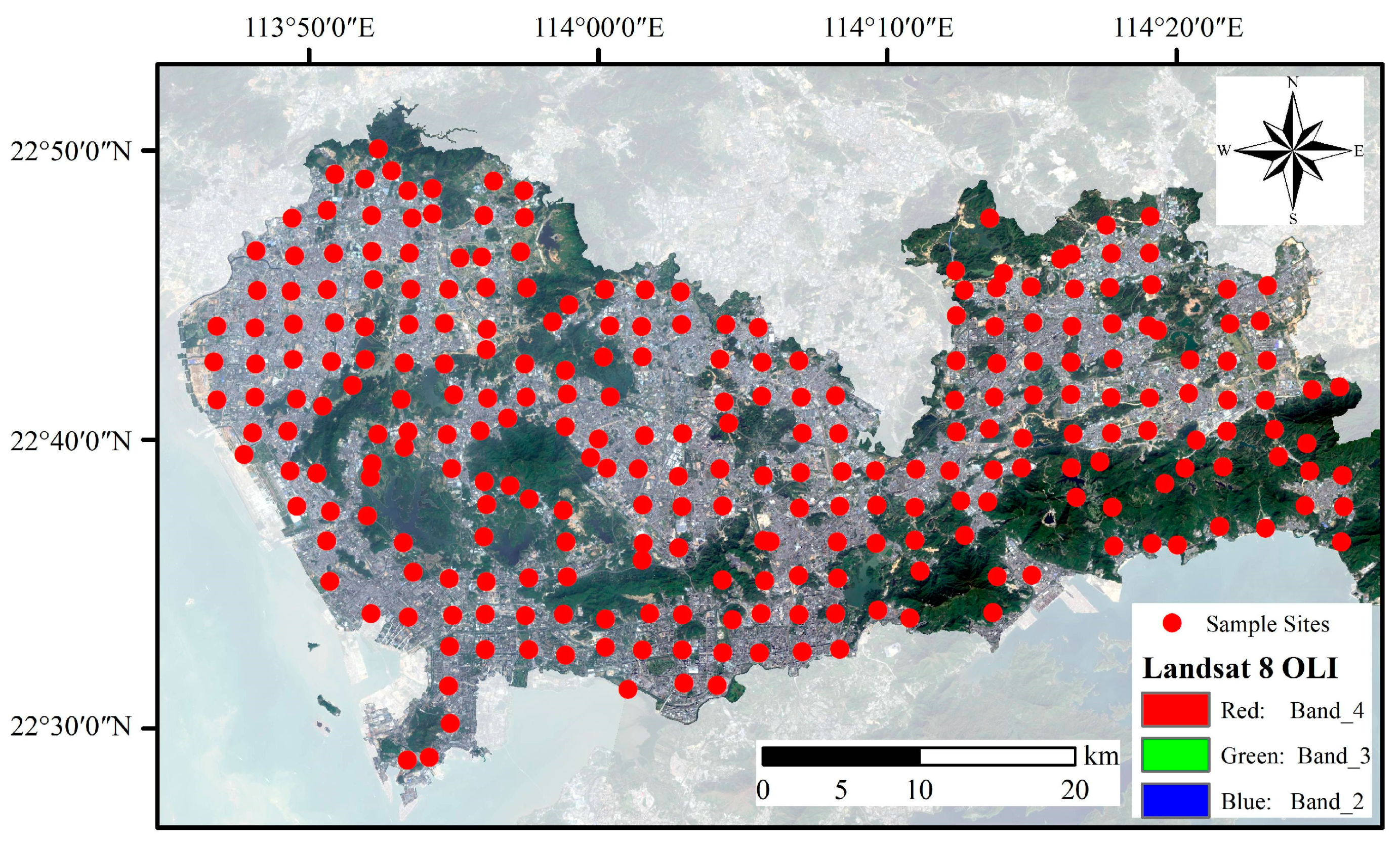
2.1. Study Area

The study area is situated in Shenzhen City, southwest China with geographic coordinates of 113°46′ E to 114°37′ E and 22°27′ N to 22°52′ N (Figure 1). This megacity is the third largest city in China and ranks tenth globally in terms of city GDP. This city has an average temperature of 22.4 °C, and the summer lasts from April to October. The region receives an average rainfall of 1933 mm, the majority of which occurs during summer. The elevation ranges from 0 to 943.7 m with a mean value of 82 m, and the average slope is 7° [33]. As classified by the Genetic Soil Classification of China (GSCC), the main soil types in this area are latosolic red soils, red soils, yellow soils, paddy soils, and coastal solonchaks [34,35]. According to the World Reference Base for Soil Resource (WRB), the main soil types are Acrisols, Cambisols, Anthrosols, and Solonchaks. In 1980, this city had a population of 0.33 million people and a GPD of 0.23 billion Yuan. At present, the city has grown to a population of 17.63 million people and a GDP of 3066.49 billion Yuan. Over the past 40 years, the increase in population and urban expansion has placed significant stress on the soil due to the presence of heavy metals. The combination of unique natural environments and extensive human activities makes this city an ideal area for studying heavy metal contaminations.

2.2. Sample Collection

In order to cover the entire area of the studied city and ensure sample representativeness, the study area was divided into grids of 2 km × 2 km. Sampling sites were randomly selected within each grid. At each site, approximately 1.5 kg of topsoil (0–20 cm) was collected, resulting in a total of 250 samples gathered in November 2016 (Figure 1). A GPS receiver was used to record the geographical coordinates of each sampling site.

2.3. Soil Spectral Measurement and Chemical Analysis

The soil samples were air-dried in the laboratory and subsequently ground to pass through a 2 mm sieve. Each sample was divided into two parts: one for spectral analysis and one for chemical analysis. The soil spectra were collected using an ASD FieldSpec® 3 portable spectroradiometer (Analytical Spectral Devices Inc., Boulder, CO, USA) with a spectral range of 350–2500 nm. Spectra were recorded with a sampling resolution of 1 nm so that each spectrum comprised reflectance at 2151 wavelengths [36]. The spectral scans were conducted in a dark room using a halogen lamp as the sole light source, positioned at a zenith angle of 45°. The fiber probe was positioned 12 cm above the sample surface at a zenith angle of 90°. A Spectralon® panel (Analytical Spectral Devices Inc., Boulder, CO, USA) with 99% reflectance was utilized to calibrate the spectrometer before measurement. The scans were performed 10 times, and the results were subsequently averaged [15]. The Cu in the soil was extracted using the diethylenetriamine penta-acetic acid method and measured using ICP-OES (PerkinElmer, Inc., Shelton, CT, USA) [37,38].

2.4. Piecewise Spectral Pretreatment

2.4.1. Traditional Spectral Pretreatment

The six widely used traditional pretreatments that were selected were as follows: mean centering (MC), Savitzky–Golay (SG) smoothing, first derivative (FD), log(1/R), multiplicative scatter correction (MSC), and standard normal variate (SNV) [15,39]. (1) MC does not directly reduce collinearity in multivariate regression models but enhances the numerical stability of certain models, such as partial least squares regression (PLSR) [40]. (2) SG smoothing uses a low-pass filter to smooth a spectrum by removing high-frequency noise and allowing low-frequency signals to pass through [41]. In this study, the size of the window (filter width) is 15 nm, and the order of the polynomials is 3. (3) FD is usually applied as a pretreatment method to remove baseline offset [42]. (4) The transformation of reflectance R into log(1/R) enhances the edges of absorption features, facilitating linearization between the spectrum and Cu content [43]. (5) MSC minimizes the influence of scattering effects [13]. (6) SNV corrects for light scatter and particle size interferences in spectral data and shares a similar function to MSC [21]. These six traditional spectral pretreatments were carried out using the PLS_toolbox (Eigenvector Research, Inc., Manson, WA, USA) in the MATLAB environment (The MathWorks, Inc., Natick, MA, USA).

2.4.2. Piecewise Spectral Pretreatment

In the traditional method, a single spectral pretreatment is used across the entire spectrum, which ranges from 350 to 2500 nm. However, different parts of the spectrum may respond differently to distinct pretreatments. In this study, the spectrum was divided into three parts: 350–1000 nm (left part), 1001–700 nm (middle part), and 1701–2500 nm (right part). The ASD FieldSpec® 3 portable spectroradiometer consists of three internal spectrometers, with interval points around 1000 and 1700 nm for each spectrometer [44]. The experiments can be divided into three strategies according to the number of pretreated spectrum parts:
(1)
One-part pretreatment strategy. Only one part of the spectrum was pretreated, leaving the other two parts untreated. These three parts we then combined to construct the Cu estimation model. Only one of the three parts (left part, middle part, and right) was pretreated using six different methods, resulting in 18 models ( C 3 1 *6 = 18). For example, only the middle part of the spectrum was pretreated with SG, leaving the left and right untreated. This one-part pretreatment method was denoted as “No–SG–No”.
(2)
Two-part pretreatment strategy. Two parts of the spectrum were pretreated, leaving one part untreated. The three parts were then merged to construct the Cu estimation model. Only two out of the three parts (left-middle, left-right, and middle-right) were pretreated using six different methods, resulting in 108 models ( C 3 2 *6*6 = 108). For example, SG was applied to the middle part and MSC to the right part, leaving the left part untreated. This two-part pretreatment method was denoted as “No–SG–MSC”.
(3)
Three-part pretreatment strategy. All three parts of the spectrum were pretreated and then merged together to construct the Cu estimation model. All three parts (left part, middle part, and right) were pretreated using six different methods, resulting in 342 models ( C 3 3 *6*6*6 = 216). For example, FD was used for the left part, SG for the middle, and MSC for the right part. This three-part pretreatment method was denoted as “FD–SG–MSC”.
The three strategies were carried out using the PLS_toolbox (Eigenvector Research, Inc., Manson, WA, USA) in the MATLAB environment (The MathWorks, Inc., Natick, MA, USA).

2.5. PLSR Models

Partial least squares regression (PLSR) is a widely used method that helps establish a correlation between soil spectra and soil properties [45,46]. First, PLSR projected the spectral data onto a low-dimensional space by maximizing the covariance between the soil spectra and Cu. Multiple regression analysis was then conducted within the low-dimensional space. The PLSR was carried out using the PLS_toolbox (Eigenvector Research, Inc.) in the MATLAB environment (The MathWorks, Inc.).
The calibration set comprised around 80% of the total samples, which equals 200 samples. Meanwhile, the validation set consisted of 50 samples. Previous studies showed that the portion of the validation samples ranged from 20% to 50%, and we decided on a 20% validation set [9,21,26,30,31]. The 20% and 80% split was based on arranging the samples in ascending order of Cu content. For every four samples, one was chosen for validation, and the remaining ones formed the calibration set. This split ensured that the validation samples were evenly distributed across the range of Cu content, effectively covering the diversity of Cu expected in future samples.
The calibration set was employed to build the PLSR models. The spectra were subjected to piecewise pretreatment described in Section 2.4.2. The number of the latent variables was determined using leave-one-out cross-validation (LOOCV).

2.6. Performancce of Models

The validation set mentioned in Section 2.5 was used to test the built model. The performance of the PLSR models was evaluated using several indicators, namely, residual predictive deviation (RPD), root mean square error of prediction (RMSEP), and coefficient of determination in prediction ( R p 2 ).

3. Results

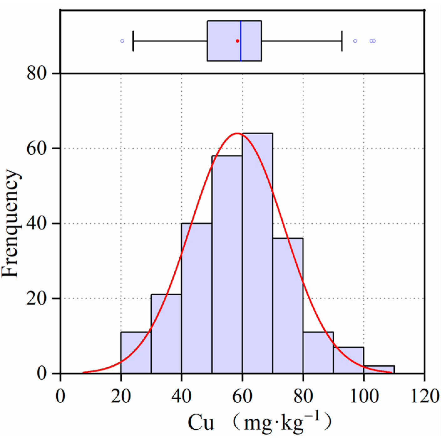
3.1. Descriptive Statistics of Soil Samples

The Cu content ranged from 20.45 mg·kg−1 to 103.24 mg·kg−1 with a mean of 58.29 mg·kg−1 (Table 1 and Figure 2). The coefficient of variation (CV) was 0.27, indicating a medium level of variability (0.1 < CV < 1.0) [47]. The skewness was close to zero at 0.13, implying a similar distribution of samples with low and high Cu contents. The kurtosis was also close to zero at 0.12, indicating that the Cu content almost showed a normal distribution. The statistical indicators for the calibration and validation sets were almost similar.

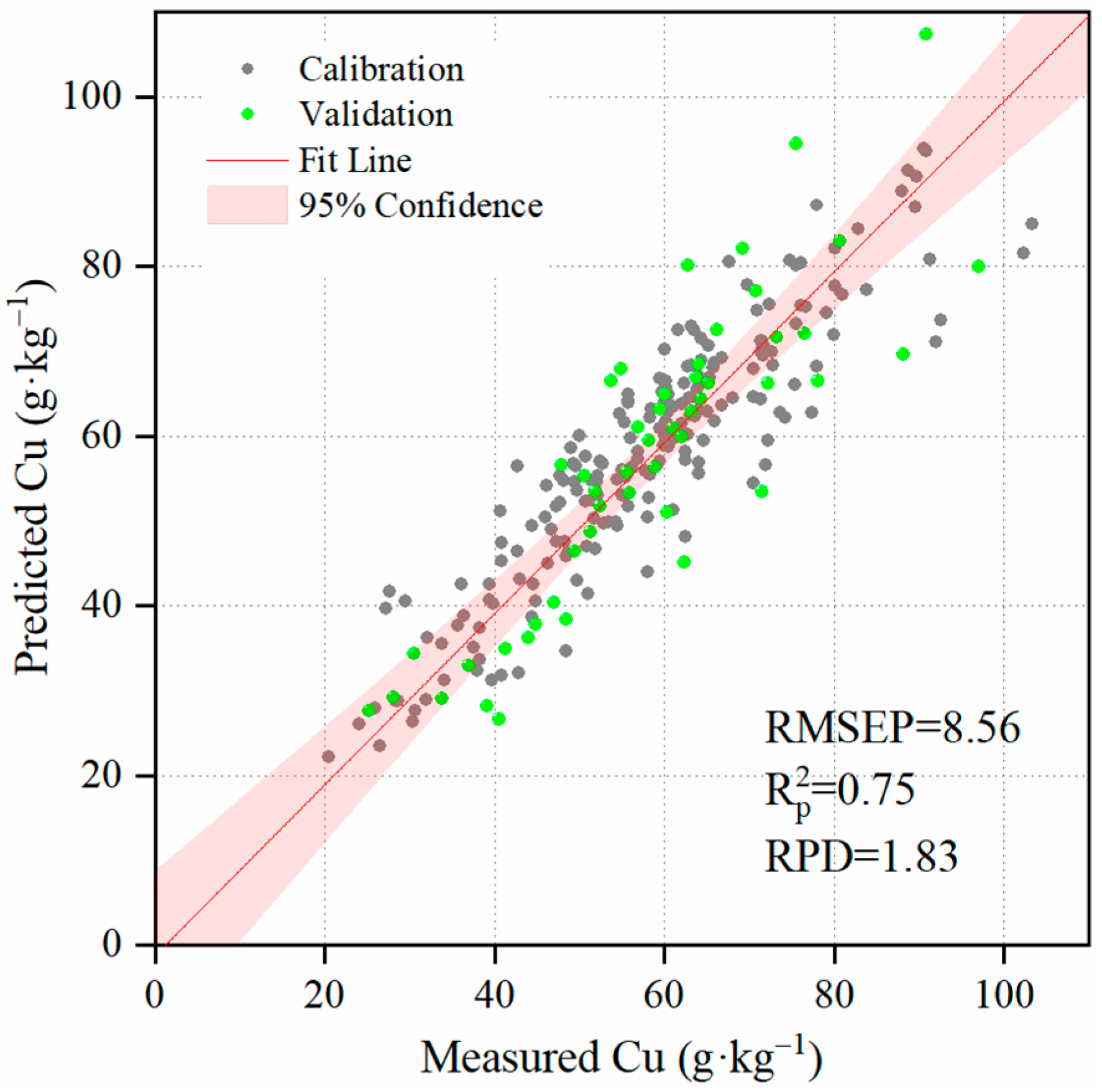
3.2. Estimation Accuracy of Cu Models with the Traditional Spectral Pretreatment

When spectral pretreatment was not applied, the Cu estimation model produced acceptable results (Figure 3). For the raw spectra, the R p 2 was 0.75, and the majority of the samples were closely aligned with the fit line within the 95% confidence area. Our results were much better than those in the study of Gholizadeh et al. [25]. The RMSEP was 8.56 mg·kg−1, and the RPD was 1.83. These two indicators suggested that the model was capable of estimating soil Cu content with reasonably satisfactory accuracy for this huge city.
When different spectral pretreatments were used for the entire wavelength of 350–2500 nm, the performance of the Cu estimation models varied (Table 2). For MC, the RMSEP decreased from 8.86 to 7.97 mg·kg−1 and the RPD increased from 1.83 to 1.96. Thus, MC contributed to enhancing the performance of the Cu estimation model. For SG and Lg, the model exhibited minimal changes. For MSC and SNV, the R p 2 decreased significantly from 0.75 to approximately 0.51–0.53 and the RPD decreased from 1.83 to approximately 1.41–1.43. For FD, the model showed poor performance, with an R p 2 of 0.09 and an RPD of 0.84.

3.3. Estimation Accuracy of Cu Models with Piecewise Pretreatment

In traditional spectral pretreatment, the entire wavelength from 350 to 2500 nm was processed uniformly. This study divided the entire wavelength into three parts: 350–1000 nm (Left, L), 1001–1700 nm (Middle, M), and 1701–2500 nm (Right, R). Each part was subjected to different spectral pretreatments. This proposed approach was referred to as piecewise pretreatment.
The number of pretreated parts varied from 1 to 3 to investigate the impact of piecewise pretreatment on the Cu estimation models.

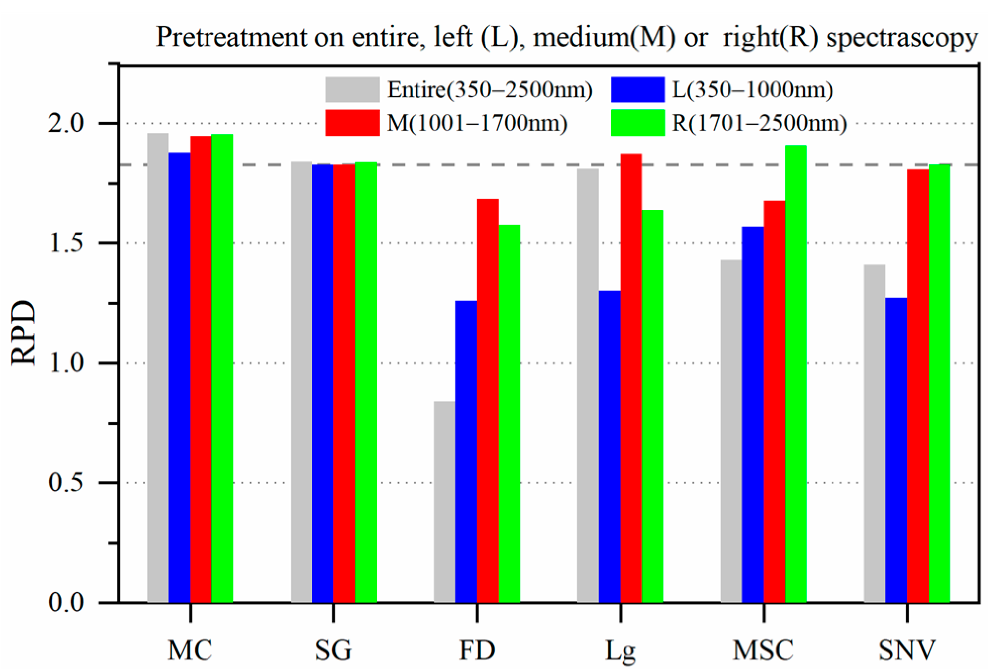
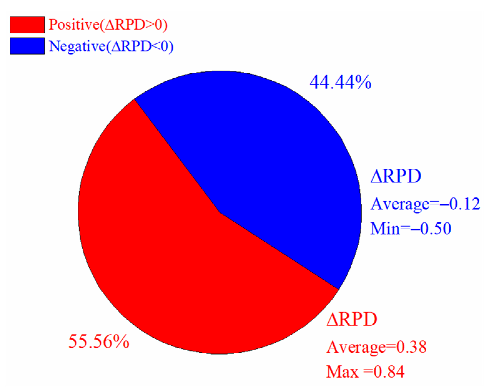
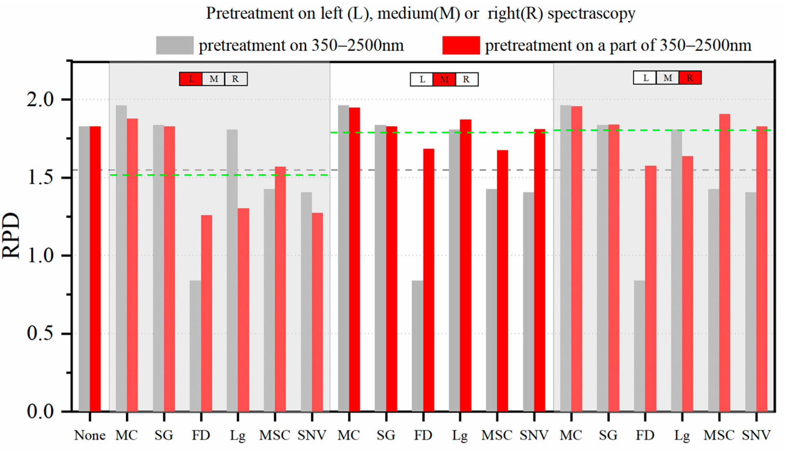
3.3.1. One Part Was Pretreated

In this section, only one part of the spectrum was pretreated, and the others were left untreated. The three parts were then combined to construct the Cu estimation model, resulting in 18 (6*3) models. The results were presented in three aspects: (i) comparisons between each pretreatment (Figure 4); (ii) comparison among left, middle, and right parts (Figure 5); and (iii) overall performance (Figure 6).
For each pretreatment, its performance differed among the three parts (Figure 4). For MC and SG, the RPD changed slightly. For FD, the RPD increased from 0.84 to 1.26, 1.68, and 1.57 for the left, middle, and right parts, respectively. The improvement was evident. For MSC, the RPD was only 1.43 when the entire spectra were pretreated but could reach 1.91 when only the right part was pretreated. For SNV, improvements were observed in the middle and right parts; however, the RPD in the left part decreased from 1.41 to 1.27. For Lg, the model’s performance was negatively impacted by pretreating the left and right parts but was slightly improved by pretreating the middle part.
In the case of the three parts (left, middle and right), the impact of pretreatment on the Cu estimation model differed (Figure 5). The mean RPD for the left, middle, and right parts was 1.52, 1.80, and 1.79, respectively. The mean RPD of the middle part was similar to that of the right part. Compared with that of the entire spectra, the mean RPD of the pretreated middle and right parts increased significantly from 1.54 to approximately 1.80 after pretreatment. For the left part, the mean RPD was 1.52, and its reduction from 1.54 to 1.52 was slight. Thus, improvements were evident in the middle and right, and almost no change happened in the left part.
Overall, 55.56% were positive, and 44.44% were negative (Figure 6). In most cases, the pretreatment of only one part performed better than the pretreatment of the entire spectra. The mean ∆RPD was 0.38 in the positive cases and only 0.12 in the negative cases. Thus, the degree of improvement was relatively higher than that of deterioration.

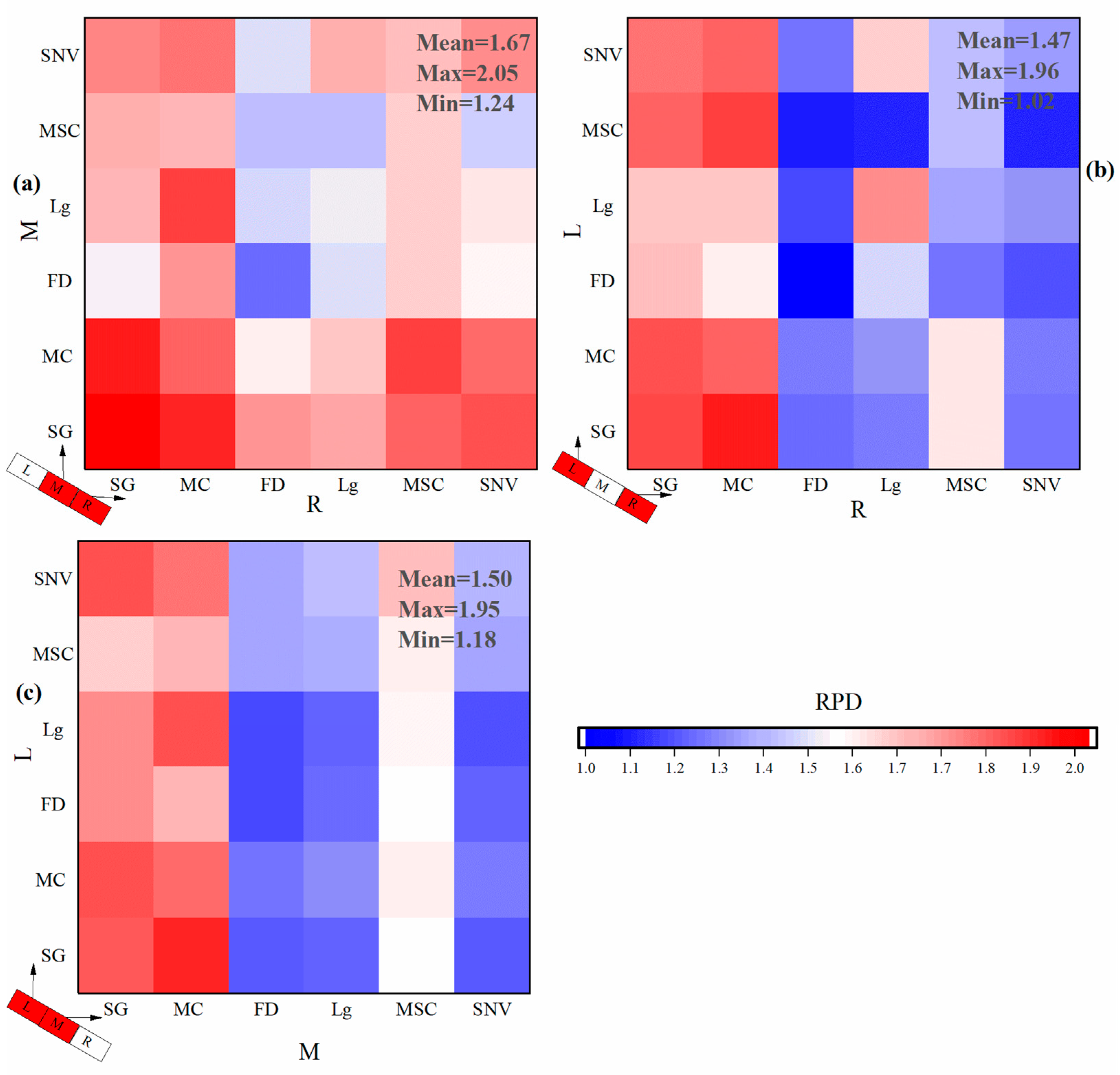
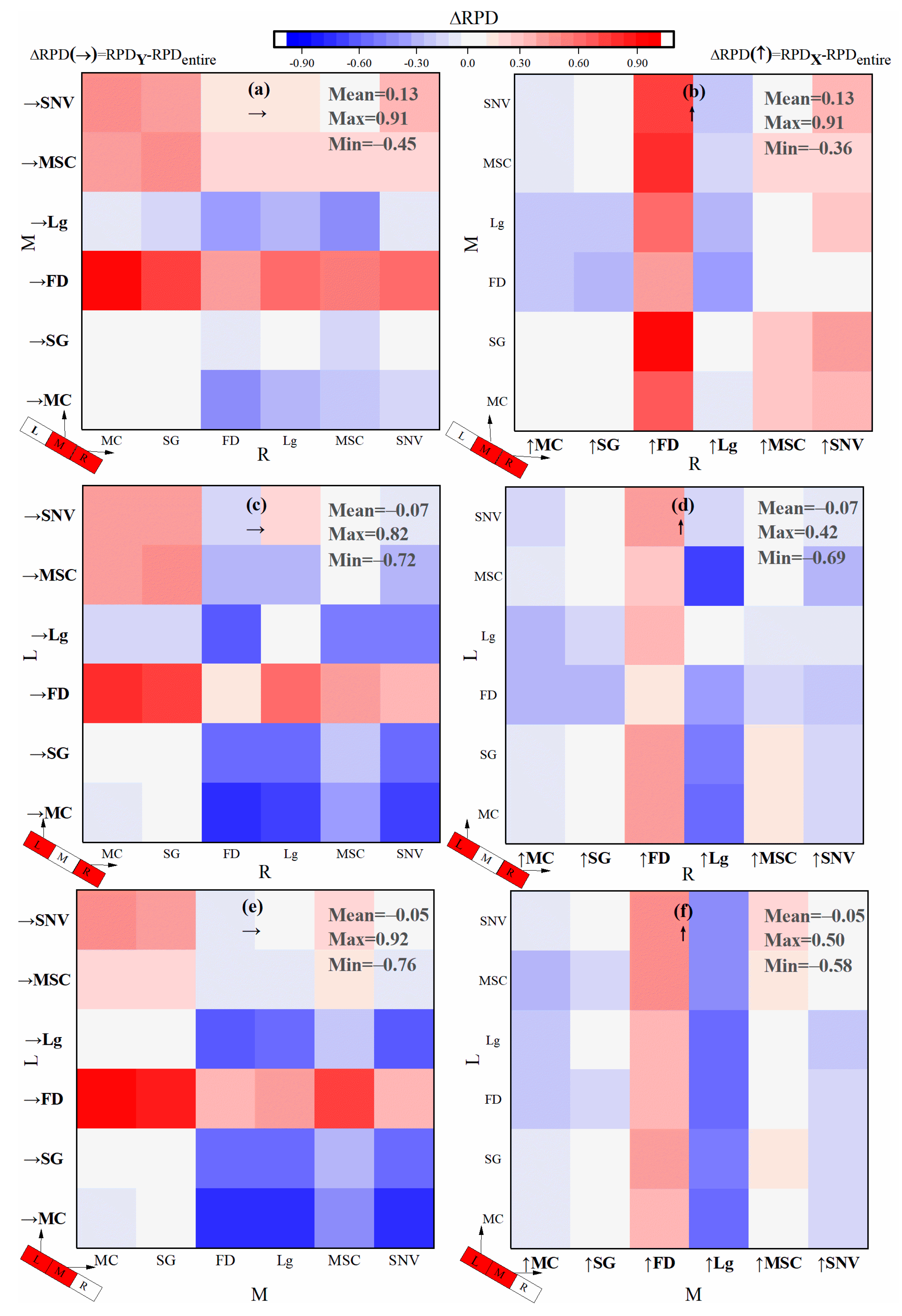
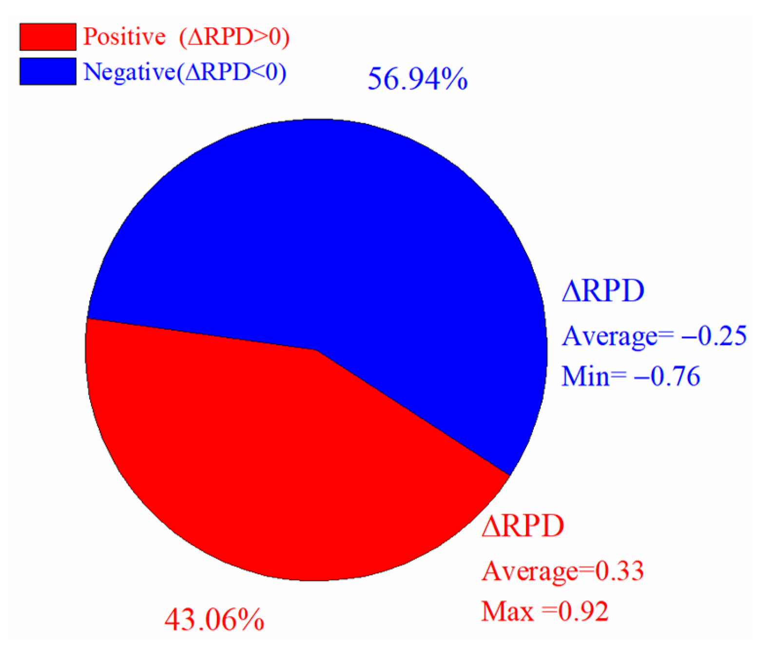
3.3.2. Two Parts Were Pretreated

In this section, two parts of the spectrum were pretreated, and the third part was left untreated. The three parts were then combined to construct the Cu estimation model, resulting in 108 (6*6*3) models. The results were presented in three aspects: (i) RPD (Figure 7), (ii) ∆RPD (Figure 8), and (iii) overall performance (Figure 9).
For RPD, the optimal performance was achieved through the pretreatment of the middle and right parts (Figure 7a). The mean RPD of the pretreatment of middle and right parts was 1.67, and the maximum RPD reached 2.05. However, the other two pretreatment combinations showed a slightly poor performance (Figure 7b,c). The mean RPD for the pretreatment of left and right parts (left-right) was 1.47 (Figure 7b). Similarly, the mean RPD for the pretreatment of left and middle parts (left-middle) was 1.50 (Figure 7c). When pretreating the entire spectrum, the RPD was 1.54. Therefore, the model experienced a slight deterioration after the pretreatment of left-right parts and left-middle parts, resulting in a decrease in RPD from 1.54 to 1.47 (left-right) and 1.50 (left-middle).
In Figure 7b,c, the left two columns were red, and the right four columns were blue. However, this phenomenon was not observed in Figure 7a. This finding indicated the following: (i) in contrast to the other four pretreatments that led to a consistently low RPD, SG and MC consistently exhibited a high RPD when the left part was pretreated. (ii) If the left part was pretreated, pretreating the right part or the middle part did not change the observed “red-blue-column” phenomenon. (iii) The disappearance of this phenomenon and the presence of a relatively high RPD were observed only when the left part was not pretreated, as illustrated in Figure 7a.
The “red-blue-column” phenomenon suggests that the left part may have a significant or potential decisive impact on spectral pretreatment. In this study, employing left pretreatment could lead to the degradation or disruption of the model. In Section 3.3.1 (Figure 5), the effect of pretreating the left part also differed from that of pretreating the middle and right parts. Hence, the pretreatment of one part exhibited some similarities to that of the two parts.
SG and MC performed well with either the entire spectra pretreatment or one-part pretreatment but not with the two-part pretreatment. When the left part was pretreated and the middle or right was pretreated with FD, Lg, MSC, and SNV (Figure 7b,c), the RPD was significantly low. Thus, the pretreatment of two parts was more complex than the pretreatment of one part.
For ∆RPD, an improvement was observed for FD, as highlighted by the red color. Meanwhile, the MC, SG, and Lg showed deterioration, as indicated by the blue color (Figure 8). For FD, a red horizontal strip appeared, as shown in Figure 8a,c,e, along with a red vertical strip, as illustrated in Figure 8b,d,f. The red strip indicated a noticeable improvement achieved by FD. The highest ∆RPD was 0.91. For MC, SG, and Lg, a blue horizontal strip appeared, as shown in Figure 8a,b,c, along with a blue vertical strip, as presented in Figure 8b,d,f. The lowest ∆RPD was −0.76.
The explanation for the red strip or blue strip might be straightforward. When pretreating the entire spectra, FD showed poor performance with an RPD of 0.84. By contrast, MC, SG, and Lg demonstrated good performance, achieving RPD values ranging from 1.81 to 1.96 (Figure 6 and Table 2). The two-part pretreatment mixed these two types (good and poor performances) of pretreatment. As a consequence, the RPD of the initially underperforming methods such as FD improved, and that of initially well-performing ones such as MC, SG, and Lg deteriorated. This finding suggested that the two-part pretreatment could be beneficial for weaker pretreatments (e.g., Lg) but ineffective for excellent pretreatments (e.g., MC).
For ∆RPD, the pretreatment of the middle and right parts (Figure 8a,b) was more effective than the other two combinations, namely, left-right (Figure 8c,d) and left-middle (Figure 8e,f). The mean ∆RPD for the middle-right combination was 0.13, and those for the left-right and left-middle combinations were −0.07 and −0.05, respectively.
Overall, 56.94% were positive, and 43.06% were negative (Figure 9). In most cases, the pretreatment of two parts would perform better than that of the entire spectrum. The mean ∆RPD was 0.33 in positive case, and −0.25 in negative case. Thus, the difference in ∆RPD may be somewhat similar.

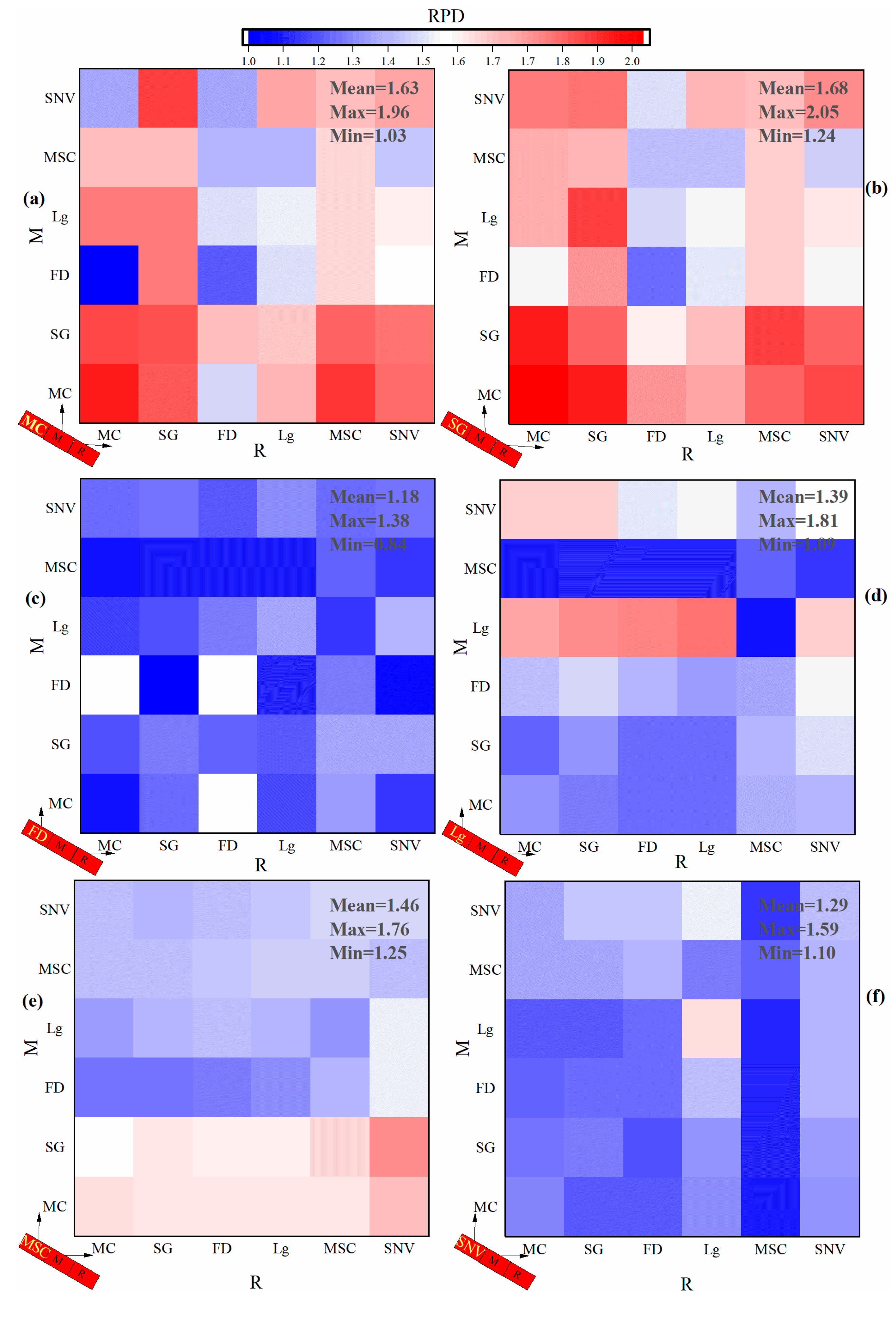
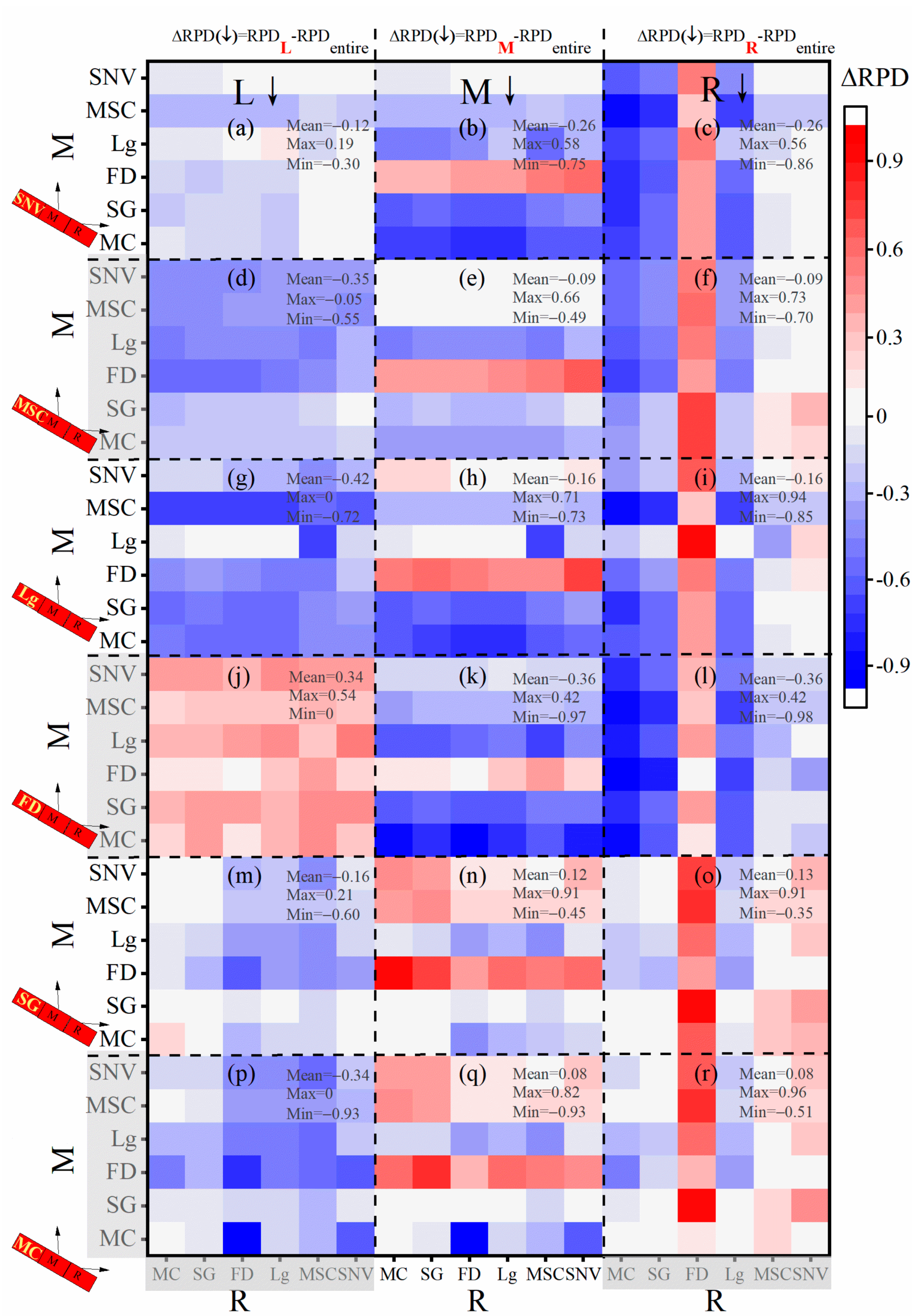
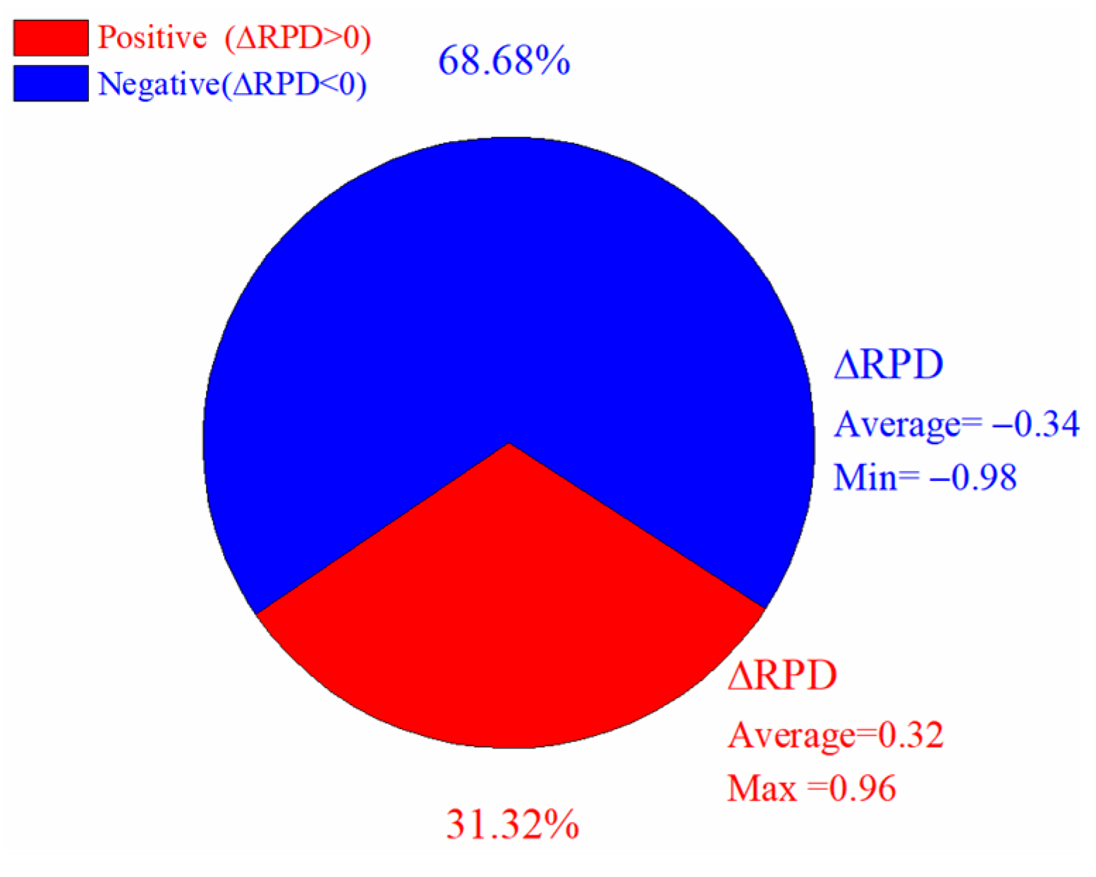
3.3.3. Three Parts Were Pretreated

In this section, three parts of the spectrum were subjected to different pretreatments and then combined to construct the Cu estimation model, resulting in 216 (6*6*6) models. The results were presented in three aspects: (i) RPD (Figure 10), (ii) ∆RPD (Figure 11), and (iii) overall performance (Figure 12).
For RPD, when the left part was pretreated with either MC or SG, the model showed good performance, indicated by a red color (Figure 10a,b). The mean RPD for the left part pretreated with MC and SG was 1.63 and 1.68, respectively. These values were relatively higher than those for the other four pretreatment methods (Figure 10c,d,e,f). For FD and SNV pretreatments, the mean RPD values were 1.18 and 1.29, respectively. Almost all blocks exhibited a blue color under these conditions (Figure 10c,f). For Lg and MSC pretreatments, the mean RPD values were 1.39 and 1.49, respectively. Some blocks were colored red (Figure 10d,e). Therefore, Lg and MSC performed better than FD and SNV.
For RPD, distinct performance outcomes were unexpectedly observed between MSC and SNV (Figure 10e,f). In theory, MSC was expected to be very similar to SNV; however, the results showed otherwise. The mean RPD of MSC was 1.46, and that of SNV was only 1.29.
For ∆RPD, FD obtained the best result (Figure 11). Visible red strips appeared in either a horizontal or vertical direction. The maximum ∆RPD for FD was 0.96, and the RPD was 1.80 (Figure 11r). As shown in Figure 11j, nearly all the blocks appeared red in color. For MC and SG, blue strips were observed, particularly the horizontal strips in Figure 11b,e,h,k, and the vertical strips in Figure 11c,f,i,l. The minimum ∆RPD was −0.98, and the RPD was only 0.98. The appearance of red and blue strips was similar to that of the two-part pretreatment in Section 3.3.2. This result also indicated that three-part pretreatment might be helpful for the weak pretreatments (e.g., FD) but useless to the excellent pretreatments (e.g., MC).
For ∆RPD, the effect of pretreating the left part was different from that of pretreating the middle and right parts (Figure 11). For the left part, most blocks were blue, indicating that their influence was negative because the ∆RPD < 0, except for FD (Figure 11a,d,g,j,m,p). For the middle and right parts, more red blocks and fewer blue blocks were observed, suggesting that the left-part pretreatment was less effective than the middle and right part pretreatments. This outcome contradicted the result for two-part pretreatment in Section 3.3.2. For FD in the left part pretreatment (Figure 10j), all blocks appeared red. This phenomenon was mainly due to the poor performance of FD for the entire spectrum, suggesting its potential for improvement under the three-part pretreatment.
Overall, 31.32% were positive and 68.68% were negative (Figure 12). In most cases, the pretreatment of the three parts performed worse than that of the entire spectrum. In the one-part and two-part pretreatments, the positive portion outweighed the negative portion. However, in three-part pretreatment, the situation was quite the opposite. The mean ∆RPD was 0.32 in positive case and −0.34 in negative case.

3.3.4. Comparison of One-Part, Two-Part, and Three-Part Strategies

For RPD, the mean value decreased as the number of pretreated parts increased (Table 3). The mean RPD value for one-part, two-part, and three-part pretreatments were 1.71, 1.55, and 1.44, respectively. In the traditional pretreatment, the mean RPD was 1.55. In terms of mean RPD, the one-part pretreatment showed significantly better performance and the two-part pretreatment demonstrated similar effectiveness to the traditional pretreatment. Meanwhile, the three-part pretreatment showed slightly lower performance than traditional pretreatment. The two-part and three-part pretreatment methods obtained the highest RPD of 2.05, slightly surpassing the performance of the traditional pretreatment and one-part pretreatment. With regard to minimum RPD, the one-part pretreatment yielded a value of 1.26, and the traditional pretreatment had a significantly lower value of 0.84.
For ∆RPD, a decrease in the positive portion and the mean ∆RPD was observed when more parts were pretreated (Table 3). The percentage of positive outcomes in ∆RPD decreased from 55.56% for the one-part pretreatment to 43.06% for the two-part pretreatment and further to 31.32% for the three-part pretreatment. The mean ∆RPD decreased slightly from 0.38 to 0.32 in positive cases and from −0.12 to −0.32 in negative cases. This decrease indicates that the Cu estimation model would perform poorly when many parts are pretreated.
Compared with the traditional method, the one-part pretreatment and two-part pretreatment proved more effective. Meanwhile, the three-part pretreatment showed a slightly reduced effectiveness. The mean RPD was 1.55 with the traditional pretreatment method. However, this value increased to 1.71 when employing the one-part pretreatment. A similar increase was observed for the positive portion and the mean ∆RPD (Table 3).

4. Discussion

4.1. Influence of Piecewise Pretreatment on Cu Estimation Model

In this study, the Cu estimation model produced acceptable results (Figure 3) with the R p 2 of 0.75 and the RMSEP of 8.86 mg·kg−1. In comparison, Liu et al. (2011) achieved a R p 2 of 0.37 for soil Cu estimation, indicating relatively lower predictability [48]. Riedel et al. (2018) only obtained a R p 2 of 0.01 using vis-NIR spectroscopy for soil Cu estimation [49]. Cheng et al. (2019) achieved a R p 2 of 0.26 for Cu estimation in suburban soils [50]. Some researchers have reported higher accuracy, with a R p 2 of 0.67 [51], 0.91 [52] and 0.92 [53]. Therefore, in comparison with previous studies, our results appear to be acceptable.
The important wavelengths utilized in the PLSR models for estimating soil Cu were identified using variable importance in projection (VIP) scores [54]. Wavelengths with VIP scores exceeding 1 were regarded as highly correlated and significant for estimating soil Cu [55]. In this study, the critical wavelengths for Cu estimation were identified within the ranges of 1031–1890 nm, 1973–2193 nm, 2213–2266 nm, and 2474–2497 nm (Figure 13). The region of 2213–2266 nm is attributed to overtones and combinations of fundamental vibrations of organic molecules, such as C–H, N–H, S–H, C=O, and O–H [18]. Some research has reported significant wavelengths at 700 nm, 1000 nm, 1400 nm, 1900 nm, and 2200 nm [25,48]. The variation in important wavelengths may be attributed to different soil parent materials and environmental conditions.
The piecewise pretreatment generally outperformed the traditional method in most cases. The traditional method applies the same pretreatment to treat the entire spectrum. Out of the six pretreatments (MC, SG, FD, Lg, MSC and SNV), only two (33.33%) demonstrated positive effects (Table 3). Previous studies also demonstrated poor performance of traditional spectral pretreatment in estimating soil Cu content [48,49]. In one-part pretreatment, 55.56% demonstrated positive effects. The mean RPD was 1.55 for the traditional method and 1.71 for the one-part pretreatment. Its higher mean RPD indicates that the one-part pretreatment performed better than the traditional method. In terms of positive portion and mean RPD, the traditional pretreatment in this study may not have been effective or the data may not be sensitive to this method. Nevertheless, employing piecewise pretreatment improved the situation and significantly enhanced the performance of the Cu estimation models. Thus, in cases where traditional pretreatments do not yield satisfactory results [19,50], we recommend the piecewise pretreatment method to obtain good outcomes.
The three types of piecewise pretreatment method—namely one-part pretreatment, two-part pretreatment, and three-part pretreatment—exhibited different performances (Figure 4, Figure 7 and Figure 10). This study indicated that the Cu estimation model is likely to perform poorly when more parts are subjected to pretreatment. The mean RPD decreased from 1.71 for the one-part to 1.55 for the two-parts, and further to 1.44 for the three-parts (Table 3). A similar decrease was observed in the positive portion. This finding suggests that pretreating one part is the best approach, a notable departure from the traditional method of using the entire spectrum. The reason is that using a few parts results in a simple and effective model. For example, in Figure 4 of FD and MSC, pretreating just one part (left, middle or right) performed better than pretreating the entire spectrum. Conversely, combing more parts led to a decline in the model’s performance. However, traditional spectral methods usually use the entire spectrum rather than specific parts [56,57].
In the piecewise pretreatment, the left part had a more negative impact than the middle and right parts. In the one-part pretreatment, the left part recorded the least favorable mean RPD of 1.52, and the left and right parts exhibited values around 1.79–1.80. In the two-part pretreatment, treating the left part would negatively impact the model performance, resulting in a poor outcome. In the three-part pretreatment, comparing Figure 7a with Figure 10a–f shows that the model’s performance usually became worse when the left part was treated. Therefore, piecewise pretreatment is ineffective for treating the left part of the spectrum. The reason is that the left part of the spectrum contains important wavelengths, as highlighted by previous research [13,51]. When the left part undergoes insufficient pretreatment using FD, MSC, or SNV, it exhibits a negative impact. This observation is supported and confirmed by the data presented in Figure 7b,c and Figure 10c–f.
In the piecewise pretreatment, less effective pretreatments such as FD, MSC, or SNV were likely to show improvement, and superior pretreatments such as SG and MC may only result in a slight improvement or, in some cases, poor outcomes. Therefore, FD, MSC, and SNV frequently showed “red strips” and SG and MC tended to display “blue strips” (Figure 8 and Figure 11). Prior studies deemed FD effective with traditional pretreatment. Gholizadeh et al. (2015) found that utilizing FD raised the R c v 2 from 0.55 to 0.78 when estimating soil Cu content [25]. Riedel et al. (2018) reported that FD was the most effective pretreatment for estimating soil Cu content using vis-NIR spectra [49]. However, in the current work, FD performed poorly for traditional pretreatment but showed promise for piecewise spectral pretreatment. A significant difference was found between MSC and SNV as depicted in Figure 7 and Figure 10e–f. However, in theory, MSC was expected to be very similar to SNV [58,59]. Table 2 shows that for the traditional method, MSC and SNV appeared to produce the same results. Thus, the piecewise pretreatment method is likely to discover the minor differences among pretreatments methods and may even amplify these distinctions.

4.2. How Piecewise Pretreatment Affects Cu Models

In piecewise pretreatment or traditional pretreatment method, MC and FD exhibits a notable contrast in performance. In this section, our discussion delves into these two pretreatments to illustrate how piecewise pretreatment influences Cu estimation models.
The effectiveness of pretreatment on Cu estimation models relies on a particular section of spectrum rather than the entire spectrum. In traditional pretreatment, the entire spectrum was pretreated, resulting in an RPD of only 0.84. This value led to the conclusion that FD was ineffective [60,61,62]. However, the previous conclusion was deemed incorrect when the one-part pretreatment method was employed (Table 4 and Figure 4). Similar occurrences were also observed for SNV and MSC. Thus, preprocessing a specific part of the spectrum may yield more convincing results than utilizing the entire spectrum.
The degree of improvement may also be influenced by the specific parts of the spectrum. For MC and SG, the left, middle, and right part exhibited high and similar performance (Figure 4). As a consequence, their improvement in piecewise pretreatment was very small (Table 4). On the contrary, the other three, namely FD, MSC, and SNV, showed more significant improvement. Furthermore, the degree of improvement was maximized at around RPD = 2, which is also optimal for traditional pretreatment. This result suggested that piecewise pretreatment may also be constrained to some extent by traditional pretreatment. These findings were also supported by the research of Wuye Yang et al. [32].
For the max RPD, the transition from one-part to three-part pretreatment resulted in a regular combination of left, middle and right part preprocessing. For FD, the optimal pretreatment combination was “No–FD–No” in the one-part method, “MC–FD–No” in the two-part method, and “MC–FD–SG” in the three-part method. First, the change from “No–FD–No” (one-part) to “MC–FD–No” (two-part) was initiated by treating the left part of spectrum with MC (Table 4). Afterward, the change from “MC–FD–No” (two-part) to “MC–FD–SG” (three-part) was employed by treating the right part of spectra with SG. Similar results were observed for MC with three combinations: “No–No–MC” (one-part), “No–MC–MC” (two-part), and “SG–MC–MC” (three-part). The same results were also observed for the remaining four. Thus, for each type of pretreatment (e.g., FD and MC), the two-part method was derived from the one-part method, and the three-part method was derived from the two-part method. Previous researchers did not report these new findings [32], making it a significant contribution to the soil field and challenging existing knowledge.
The piecewise pretreatment aims to choose effective pretreatment methods and remove ineffective ones to optimize the performance of Cu estimation models. Conclusions can be drawn from these two aspects: (i) in the one-part pretreatment, the optimal one among the three parts of the spectrum was chosen for pretreatment, leaving the remaining two parts unchanged (Figure 4 and Table 4). In the two-part method and three-part method, additional optimal pretreatment was applied to handle the remaining two parts. (ii) If a traditional pretreatment such as FD (“FD–FD–FD”) is ineffective, its impact on specific parts of the spectrum can be eliminated and it can be replaced by alternative pretreatment methods, such as “MC–FD–SG”. Combinations involving MC and SG were the most frequently employed to maximize RPD. This choice might be based on the initial good performance of MC and SG in the traditional approach. Compared with traditional spectral pretreatment [63], piecewise pretreatment is more reasonable and effective in theory.

5. Conclusions

In this study, the vis-NIR spectrum was divided into different parts to investigate how pretreating these specific parts affects the modelling of soil Cu estimation. On the basis of our results, the following conclusions were drawn: (i) piecewise pretreatment generally outperformed the traditional method in most cases; (ii) piecewise pretreatment chose effective pretreatment methods for each part and removed ineffective ones to optimize the performance of Cu estimation models; (iii) in piecewise pretreatment, less effective traditional pretreatments such as FD, MSC, or SNV are unlikely to show improvement, and superior traditional pretreatments like SG and MC may only result in a slight improvement or, in some cases, poor outcomes.
Although we have achieved success in deeply investigating how piecewise spectral pretreatment influences the Cu modelling, further improvement in soil Cu estimation is still possible. Although our study focused on a large area of the city, our strategy could also be applicable to small areas and farmland.

Author Contributions

Conceptualization, Y.L. and Y.C.; methodology, T.S.; software, Z.L.; validation, K.G., X.L. and T.Q.; formal analysis, Y.L.; investigation, T.S.; resources, Y.C.; data curation, S.Z.; writing—original draft preparation, T.S.; writing—review and editing, Y.C.; visualization, Y.L.; supervision, D.Z. and X.Z.; project administration, Y.L.; funding acquisition, Y.L. All authors have read and agreed to the published version of the manuscript.

Funding

This research was funded by Guangzhou Science and Technology Plan Project (202102020416), and Philosophy and Social Sciences Fund of the 13th Five-year Plan of Guangdong Province of China (GD20YGL11).

Data Availability Statement

The original contributions presented in the study are included in the article, further inquiries can be directed to the corresponding author.

Acknowledgments

We express our gratitude to the reviewers for offering valuable comments that have enhanced the quality of this paper. We also want to extend our significant appreciation to all the colleagues who provided essential assistance in this work.

Conflicts of Interest

The authors declare no conflicts of interest. Authors Xiaojin Liang and Tianqi Qiu were employed by the company Guangzhou Urban Planning & Design Survey Research Institute Co., Ltd. The remaining authors declare that the research was conducted in the absence of any commercial or financial relationships that could be construed as a potential conflict of interest.

References

  1. Xu, J.; Liu, C.; Hsu, P.-C.; Zhao, J.; Wu, T.; Tang, J.; Liu, K.; Cui, Y. Remediation of heavy metal contaminated soil by asymmetrical alternating current electrochemistry. Nat. Commun. 2019, 10, 2440. [Google Scholar] [CrossRef]
  2. Hou, D.; O’Connor, D.; Igalavithana, A.D.; Alessi, D.S.; Luo, J.; Tsang, D.C.; Sparks, D.L.; Yamauchi, Y.; Rinklebe, J.; Ok, Y.S. Metal contamination and bioremediation of agricultural soils for food safety and sustainability. Nat. Rev. Earth Environ. 2020, 1, 366–381. [Google Scholar] [CrossRef]
  3. Zhang, X.; Yan, L.; Liu, J.; Zhang, Z.; Tan, C. Removal of Different Kinds of Heavy Metals by Novel PPG-nZVI Beads and Their Application in Simulated Stormwater Infiltration Facility. Appl. Sci. 2019, 9, 4213. [Google Scholar] [CrossRef]
  4. Alengebawy, A.; Abdelkhalek, S.T.; Qureshi, S.R.; Wang, M.-Q. Heavy metals and pesticides toxicity in agricultural soil and plants: Ecological risks and human health implications. Toxics 2021, 9, 42. [Google Scholar] [CrossRef] [PubMed]
  5. Nriagu, J.O. A history of global metal pollution. Science 1996, 272, 223. [Google Scholar] [CrossRef]
  6. Soliman, M.M.; Hesselberg, T.; Mohamed, A.A.; Renault, D. Trophic transfer of heavy metals along a pollution gradient in a terrestrial agro-industrial food web. Geoderma 2022, 413, 115748. [Google Scholar] [CrossRef]
  7. Chary, N.S.; Kamala, C.; Raj, D.S.S. Assessing risk of heavy metals from consuming food grown on sewage irrigated soils and food chain transfer. Ecotoxicol. Environ. Saf. 2008, 69, 513–524. [Google Scholar] [CrossRef]
  8. Shi, T.; Liu, H.; Chen, Y.; Fei, T.; Wang, J.; Wu, G. Spectroscopic Diagnosis of Arsenic Contamination in Agricultural Soils. Sensors 2017, 17, 1036. [Google Scholar] [CrossRef] [PubMed]
  9. Li, S.; Visscarra Rossel, R.A.; Webster, R. The cost-effectiveness of reflectance spectroscopy for estimating soil organic carbon. Eur. J. Soil Sci. 2022, 73, e13202. [Google Scholar] [CrossRef]
  10. Kuang, B.; Mouazen, A.M. Influence of the number of samples on prediction error of visible and near infrared spectroscopy of selected soil properties at the farm scale. Eur. J. Soil Sci. 2012, 63, 421–429. [Google Scholar] [CrossRef]
  11. Dor, E.B.; Granot, A.; Wallach, R.; Francos, N.; Pearlstein, D.H.; Efrati, B.; Borůvka, L.; Gholizadeh, A.; Schmid, T. Exploitation of the SoilPRO®(SP) apparatus to measure soil surface reflectance in the field: Five case studies. Geoderma 2023, 438, 116636. [Google Scholar] [CrossRef]
  12. Viscarra Rossel, R.A.; Lobsey, C.R.; Sharman, C.; Flick, P.; McLachlan, G. Novel soil profile sensing to monitor organic C stocks and condition. Environ. Sci. Technol. 2017, 51, 5630–5641. [Google Scholar] [CrossRef] [PubMed]
  13. Shi, T.; Chen, Y.; Liu, Y.; Wu, G. Visible and near-infrared reflectance spectroscopy—An alternative for monitoring soil contamination by heavy metals. J. Hazard. Mater. 2014, 265, 166–176. [Google Scholar] [CrossRef] [PubMed]
  14. Viscarra Rossel, R.A.; Behrens, T.; Ben-Dor, E.; Chabrillat, S.; Dematte, J.A.M.; Ge, Y.; Gomez, C.; Guerrero, C.; Peng, Y.; Ramirez-Lopez, L.; et al. Diffuse reflectance spectroscopy for estimating soil properties: A technology for the 21st century. Eur. J. Soil Sci. 2022, 73, e13271. [Google Scholar] [CrossRef]
  15. Liu, Y.; Liu, Y.; Chen, Y.; Zhang, Y.; Shi, T.; Wang, J.; Hong, Y.; Fei, T.; Zhang, Y. The Influence of Spectral Pretreatment on the Selection of Representative Calibration Samples for Soil Organic Matter Estimation Using Vis-NIR Reflectance Spectroscopy. Remote Sens. 2019, 11, 450. [Google Scholar] [CrossRef]
  16. Viscarra Rossel, R.A.; Cattle, S.R.; Ortega, A.; Fouad, Y. In situ measurements of soil colour, mineral composition and clay content by vis-NIR spectroscopy. Geoderma 2009, 150, 253–266. [Google Scholar] [CrossRef]
  17. Viscarra Rossel, R.A.; Webster, R. Discrimination of Australian soil horizons and classes from their visible–near infrared spectra. Eur. J. Soil Sci. 2011, 62, 637–647. [Google Scholar] [CrossRef]
  18. Stenberg, B.; Viscarra Rossel, R.A.; Mouazen, A.M.; Wetterlind, J. Chapter five-visible and near infrared spectroscopy in soil science. Adv. Agron. 2010, 107, 163–215. [Google Scholar]
  19. Xiao, Q.; Tang, W.; Zhang, C.; Zhou, L.; Feng, L.; Shen, J.; Yan, T.; Gao, P.; He, Y.; Wu, N. Spectral preprocessing combined with deep transfer learning to evaluate chlorophyll content in cotton leaves. Plant Phenomics 2022, 2022, 9813841. [Google Scholar] [CrossRef]
  20. Gholizadeh, A.; Borůvka, L.; Saberioon, M.; Vašát, R. Visible, near-infrared, and mid-infrared spectroscopy applications for soil assessment with emphasis on soil organic matter content and quality: State-of-the-art and key issues. Appl. Spectrosc. 2013, 67, 1349–1362. [Google Scholar] [CrossRef]
  21. Gholizadeh, A.; Carmon, N.; Klement, A.; Ben-Dor, E.; Borůvka, L. Agricultural Soil Spectral Response and Properties Assessment: Effects of Measurement Protocol and Data Mining Technique. Remote Sens. 2017, 9, 1078. [Google Scholar] [CrossRef]
  22. Peng, X.; Shi, T.; Song, A.; Chen, Y.; Gao, W. Estimating Soil Organic Carbon Using VIS/NIR Spectroscopy with SVMR and SPA Methods. Remote Sens. 2014, 6, 2699–2717. [Google Scholar] [CrossRef]
  23. Ba, Y.; Liu, J.; Han, J.; Zhang, X. Application of Vis-NIR spectroscopy for determination the content of organic matter in saline-alkali soils. Spectrochim. Acta Part A Mol. Biomol. Spectrosc. 2020, 229, 117863. [Google Scholar] [CrossRef] [PubMed]
  24. Barra, I.; Haefele, S.M.; Sakrabani, R.; Kebede, F. Soil spectroscopy with the use of chemometrics, machine learning and pre-processing techniques in soil diagnosis: Recent advances—A review. Trac-Trends Anal. Chem. 2021, 135, 116166. [Google Scholar] [CrossRef]
  25. Gholizadeh, A.; Borůvka, L.; Saberioon, M.M.; Kozák, J.; Vašát, R.; Němeček, K. Comparing different data preprocessing methods for monitoring soil heavy metals based on soil spectral features. Soil Water Res. 2015, 10, 218–227. [Google Scholar] [CrossRef]
  26. Dotto, A.C.; Diniz Dalmolin, R.S.; Grunwald, S.; ten Caten, A.; Pereira Filho, W. Two preprocessing techniques to reduce model covariables in soil property predictions by Vis-NIR spectroscopy. Soil Tillage Res. 2017, 172, 59–68. [Google Scholar] [CrossRef]
  27. Vasques, G.; Grunwald, S.; Sickman, J. Comparison of multivariate methods for inferential modeling of soil carbon using visible/near-infrared spectra. Geoderma 2008, 146, 14–25. [Google Scholar] [CrossRef]
  28. Nawar, S.; Buddenbaum, H.; Hill, J.; Kozak, J.; Mouazen, A.M. Estimating the soil clay content and organic matter by means of different calibration methods of vis-NIR diffuse reflectance spectroscopy. Soil Tillage Res. 2016, 155, 510–522. [Google Scholar] [CrossRef]
  29. Yu, S.; Huan, K.W.; Liu, X.X.; Wang, L.; Cao, X.W. Quantitative model of near infrared spectroscopy based on pretreatment combined with parallel convolution neural network. Infrared Phys. Technol. 2023, 132, 104730. [Google Scholar] [CrossRef]
  30. Dotto, A.C.; Diniz Dalmolin, R.S.; ten Caten, A.; Grunwald, S. A systematic study on the application of scatter-corrective and spectral-derivative preprocessing for multivariate prediction of soil organic carbon by Vis-NIR spectra. Geoderma 2018, 314, 262–274. [Google Scholar] [CrossRef]
  31. Wang, Z.; Chen, S.C.; Lu, R.; Zhang, X.L.; Ma, Y.X.; Shi, Z. Non-linear memory-based learning for predicting soil properties using a regional vis-NIR spectral library. Geoderma 2024, 441, 116752. [Google Scholar] [CrossRef]
  32. Yang, W.; Xiong, Y.; Xu, Z.; Li, L.; Du, Y. Piecewise preprocessing of near-infrared spectra for improving prediction ability of a PLS model. Infrared Phys. Technol. 2022, 126, 104359. [Google Scholar] [CrossRef]
  33. Peng, Q.Z.; Tang, L.; Chen, J.; Wu, Y.L.; Chen, X.Z. Study on the Evolution of Construction Land Slope Spectrum in Shenzhen during 2000–2015. J. Nat. Resour. 2018, 33, 2200–2212. [Google Scholar]
  34. Zhang, W.; Xu, A.; Zhang, R.; Ji, H. Review of Soil Classification and Revision of China Soil Classification System. Sci. Agric. Sin. 2014, 47, 3214–3230. [Google Scholar]
  35. Lin, T.; Zhao, S.H.; Xi, X.P.; Yang, K.; Luo, F. Environmental Background Values of Heavy Metals and Physicochemical Properties in Different Soils in Shenzhen. Environ. Sci. 2021, 42, 3518–3526. [Google Scholar]
  36. Mousavi, F.; Abdi, E.; Ghalandarzadeh, A.; Bahrami, H.A.; Majnounian, B.; Ziadi, N. Diffuse reflectance spectroscopy for rapid estimation of soil Atterberg limits. Geoderma 2020, 361, 114083. [Google Scholar] [CrossRef]
  37. Wang, C.; Yang, Z.; Yuan, X.; Browne, P.; Chen, L.; Ji, J. The influences of soil properties on Cu and Zn availability in soil and their transfer to wheat t (Triticum aestivum L.) in the Yangtze River delta region, China. Geoderma 2013, 193, 131–139. [Google Scholar] [CrossRef]
  38. Lindsay, W.L.; Norvell, W.A. Development of a DTPA Soil Test for Zinc, Iron, Manganese, and Copper1. Soil Sci. Soc. Am. J. 1978, 42, 421–428. [Google Scholar] [CrossRef]
  39. Rinnan, Å.; Berg, F.V.D.; Engelsen, S.B. Review of the most common pre-processing techniques for near-infrared spectra. TrAC Trends Anal. Chem. 2009, 28, 1201–1222. [Google Scholar] [CrossRef]
  40. Echambadi, R.; Hess, J.D. Mean-centering does not alleviate collinearity problems in moderated multiple regression models. Mark. Sci. 2007, 26, 438–445. [Google Scholar] [CrossRef]
  41. Hook, J. Smoothing non-smooth systems with low-pass filters. Phys. D Nonlinear Phenom. 2014, 269, 76–85. [Google Scholar] [CrossRef]
  42. Shetty, N.; Gislum, R. Quantification of fructan concentration in grasses using NIR spectroscopy and PLSR. Field Crops Res. 2011, 120, 31–37. [Google Scholar] [CrossRef]
  43. West, J.B.; Bowen, G.J.; Dawson, T.E.; Tu, K.P. Isoscapes: Understanding Movement, Pattern, and Process on Earth through Isotope Mapping; Springer: Dordrecht, The Netherlands, 2009; Volume 3, p. 76. [Google Scholar]
  44. Elmer, K.; Soffer, R.; Arroyo-Mora, J.P.; Kalacska, M. ASDToolkit: A Novel MATLAB Processing Toolbox for ASD Field Spectroscopy Data. Data 2020, 5, 96. [Google Scholar] [CrossRef]
  45. Goodarzi, M.; Sharma, S.; Ramon, H.; Saeys, W. Multivariate calibration of NIR spectroscopic sensors for continuous glucose monitoring. TrAC Trends Anal. Chem. 2015, 67, 147–158. [Google Scholar] [CrossRef]
  46. Della Riccia, G.; Del Zotto, S. A multivariate regression model for detection of fumonisins content in maize from near infrared spectra. Food Chem. 2013, 141, 4289–4294. [Google Scholar]
  47. Yang, Q.; Jiang, Z.; Li, W.; Li, H. Prediction of soil organic matter in peak-cluster depression region using kriging and terrain indices. Soil Tillage Res. 2014, 144, 126–132. [Google Scholar] [CrossRef]
  48. Liu, Y.; Li, W.; Wu, G.; Xu, X. Feasibility of estimating heavy metal contaminations in floodplain soils using laboratory-based hyperspectral data—A case study along Le’an River, China. Geo-Spat. Inf. Sci. 2011, 14, 10–16. [Google Scholar] [CrossRef]
  49. Riedel, F.; Denk, M.; Müller, I.; Barth, N.; Glässer, C. Prediction of soil parameters using the spectral range between 350 and 15,000 nm: A case study based on the Permanent Soil Monitoring Program in Saxony, Germany. Geoderma 2018, 315, 188–198. [Google Scholar] [CrossRef]
  50. Cheng, H.; Shen, R.; Chen, Y.; Wan, Q.; Shi, T.; Wang, J.; Wan, Y.; Hong, Y.; Li, X. Estimating heavy metal concentrations in suburban soils with reflectance spectroscopy. Geoderma 2019, 336, 59–67. [Google Scholar] [CrossRef]
  51. Wu, Y.; Chen, J.; Ji, J.; Gong, P.; Liao, Q.; Tian, Q.; Ma, H. A mechanism study of reflectance spectroscopy for investigating heavy metals in soils. Soil Sci. Soc. Am. J. 2007, 71, 918–926. [Google Scholar] [CrossRef]
  52. Malley, D.F.; Williams, P.C. Use of near-infrared reflectance spectroscopy in prediction of heavy metals in freshwater sediment by their association with organic matter. Environ. Sci. Technol. 1997, 31, 3461–3467. [Google Scholar] [CrossRef]
  53. Song, Y.; Li, F.; Yang, Z.; Ayoko, G.A.; Frost, R.L.; Ji, J. Diffuse reflectance spectroscopy for monitoring potentially toxic elements in the agricultural soils of Changjiang River Delta, China. Appl. Clay Sci. 2012, 64, 75–83. [Google Scholar] [CrossRef]
  54. Chong, I.G.; Jun, C.H. Performance of some variable selection methods when multicollinearity is present. Chemom. Intell. Lab. Syst. 2005, 78, 103–112. [Google Scholar] [CrossRef]
  55. Trap, J.; Bureau, F.; Perez, G.; Aubert, M. PLS-regressions highlight litter quality as the major predictor of humus form shift along forest maturation. Soil Biol. Biochem. 2013, 57, 969–971. [Google Scholar] [CrossRef]
  56. Xie, X.L.; Pan, X.Z.; Sun, B. Visible and Near-Infrared Diffuse Reflectance Spectroscopy for Prediction of Soil Properties near a Copper Smelter. Pedosphere 2012, 22, 351–366. [Google Scholar] [CrossRef]
  57. Pyo, J.; Hong, S.M.; Kwon, Y.S.; Kim, M.S.; Cho, K.H. Estimation of heavy metals using deep neural network with visible and infrared spectroscopy of soil. Sci. Total Environ. 2020, 741, 140162. [Google Scholar] [CrossRef] [PubMed]
  58. Dhanoa, M.; Lister, S.; Sanderson, R.; Barnes, R. The Link between Multiplicative Scatter Correction (MSC) and Standard Normal Variate (SNV) Transformations of NIR Spectra. J. Near Infrared Spectrosc. 1994, 2, 43–47. [Google Scholar] [CrossRef]
  59. Candolfi, A.; De Maesschalck, R.; Jouan-Rimbaud, D.; Hailey, P.A.; Massart, D.L. The influence of data pre-processing in the pattern recognition of excipients near-infrared spectra. J. Pharm. Biomed. Anal. 1999, 21, 115–132. [Google Scholar] [CrossRef]
  60. Chang, C.-W.; Laird, D.A. Near-infrared reflectance spectroscopic analysis of soil C and N. Soil Sci. 2002, 167, 110–116. [Google Scholar] [CrossRef]
  61. Xu, D.Y.; Chen, S.C.; Xu, H.Y.; Wang, N.; Zhou, Y.; Shi, Z. Data fusion for the measurement of potentially toxic elements in soil using portable spectrometers. Environ. Pollut. 2020, 263, 114649. [Google Scholar] [CrossRef]
  62. Camargo, L.A.; Marques, J., Jr.; Barron, V.; Ferracciu Alleoni, L.R.; Pereira, G.T.; Teixeira, D.D.B.; Rabelo de Souza Bahia, A.S. Predicting potentially toxic elements in tropical soils from iron oxides, magnetic susceptibility and diffuse reflectance spectra. Catena 2018, 165, 503–515. [Google Scholar] [CrossRef]
  63. An, C.; Yan, X.; Lu, C.; Zhu, X. Effect of spectral pretreatment on qualitative identification of adulterated bovine colostrum by near-infrared spectroscopy. Infrared Phys. Technol. 2021, 118, 103869. [Google Scholar] [CrossRef]
Figure 1. Maps that show the positions of the sampling sites and the landscapes, as indicated by a Landsat 8 OLI image with a composition of bands 4 (red), 3 (green), and 2 (blue).
Land 13 00517 g001
Figure 2. Boxplot and histogram of Cu content of all samples. Repoint (·) denotes the mean value. Blue line (|) denotes the median value. Hollow circle () denotes the outliers. The black box denotes the interquartile range.
Land 13 00517 g002
Figure 3. Comparison of soil Cu content between estimated and measured values using spectroscopy models without spectral pretreatment. RMSEP denotes root mean square error of prediction. R p 2 denotes coefficient of determination in prediction. RPD denotes the residual predictive deviation.
Land 13 00517 g003
Figure 4. The RPD of the soil Cu estimation model when only one part of the soil spectra was pretreated. The grey bar denotes that the entire spectra was pretreated. MC denotes mean centering. SG denotes Savitzky–Golay smoothing. FD denotes the first derivative. Lg denotes log(1/R). MSC denotes multiplicative scatter correction. SNV denotes standard normal variate.
Land 13 00517 g004
Figure 5. The RPD of soil Cu estimation model when only one part (left, middle, and right) of the soil spectra was pretreated. The green dotted line (---) denotes the mean RPD when only one part was pretreated. The grey dotted line (---) denotes the mean RPD when the entire spectra was pretreated. MC denotes mean centering. SG denotes Savitzky–Golay smoothing. FD denotes the first derivative. Lg denotes log(1/R). MSC denotes multiplicative scatter correction. SNV denotes standard normal variate.
Land 13 00517 g005
Figure 6. Overall performance of ∆RPD when only one part of the spectra was pretreated.
Land 13 00517 g006
Figure 7. The RPD of soil Cu estimation model when two parts of the spectra were pretreated. Figure (a) denotes that the middle and right parts were pretreated. Figure (b) denotes that the left and right parts were pretreated. Figure (c) denotes that the left and middle parts were pretreated. L, M, and R denote the left, middle, and right parts of the spectra, respectively. MC denotes mean centering. SG denotes Savitzky–Golay smoothing. FD denotes the first derivative. Lg denotes log(1/R). MSC denotes multiplicative scatter correction. SNV denotes standard normal variate.
Land 13 00517 g007
Figure 8. The change in the RPD when two parts of the spectra were pretreated. The ∆RPD is calculated by subtracting the RPD of the two-part pretreatment (as shows in Figure 7) from the RPD of the entire spectra pretreatment (traditional pretreatment). Subtraction can be performed along both the Y and X axes. In other words, subtracting Figure 7a along the Y-axis results in (a), while subtracting along the X-axis produced (b). (a,c,e) are derived from the Y-axis. (b,d,f) are obtained from the X-axis. MC denotes mean centering. SG denotes Savitzky–Golay smoothing. FD denotes the first derivative. Lg denotes log(1/R). MSC denotes multiplicative scatter correction. SNV denotes standard normal variate.
Land 13 00517 g008
Figure 9. Overall performance of ∆RPD when two parts of the spectra were pretreated.
Land 13 00517 g009
Figure 10. The RPD of soil Cu estimation model when three parts of the soil spectra were pretreated. Figure (af) denotes that the left part was pretreated with MC, SG, FD, Lg, MSC, and SNV, respectively. Then the middle and right parts were pretreated. MC denotes mean centering. SG denotes Savitzky–Golay smoothing. FD denotes the first derivative. Lg denotes log(1/R). MSC denotes multiplicative scatter correction. SNV denotes standard normal variate.
Land 13 00517 g010
Figure 11. The change in the RPD when three parts of the spectra were pretreated. ∆RPD is calculated by subtracting the RPD of three-part pretreatment (as shown in Figure 10) from that of the entire spectra pretreatment (traditional pretreatment). Subtraction can be performed along the left, middle, and right dimensions. In other words, subtracting Figure 10 along the left dimension results in Figure (a,d,g,j,m,p). Similarly, subtracting Figure 10 along the middle dimension results in Figure (b,e,h,k,n,q). Subtracting Figure 10 along the right dimension results in Figure (c,f,i,l,o,r). MC denotes mean centering. SG denotes Savitzky–Golay smoothing. FD denotes the first derivative. Lg denotes log(1/R). MSC denotes multiplicative scatter correction. SNV denotes standard normal variate.
Land 13 00517 g011
Figure 12. Overall performance of ∆RPD when three parts of the spectra were pretreated.
Land 13 00517 g012
Figure 13. Variable importance projection (VIP) scores associated with the cross-validation of partial least squares regression model for soil Cu estimation. The threshold for VIP was set to 1 (red line).
Land 13 00517 g013
Table 1. The descriptive statistics of 250 soil samples for the calibration and validation sets.
SampleNumberCu (mg·kg−1)
Range 1MinMaxMedianMeanStd 2CV 3SkewnessKurtosis
Total25082.7920.45103.2459.4458.2915.570.270.130.12
Calibration20082.7920.45103.2459.4458.2915.600.270.130.15
Validation5071.8525.2197.0659.1858.3015.630.270.130.12
1 Range denotes the difference between the maximum and minimum observations. 2 Std denotes standard deviation. 3 CV denotes coefficient of variation.
Table 2. Summary statistics for soil Cu estimation models with traditional spectral pretreatments.
Spectral PretreatmentCalibrationValidationLVs
R c v 2 R M S E c v R p 2 RMSEPRPDRPIQ
None0.649.720.758.861.832.076
MC0.678.900.747.971.962.226
SG0.649.750.758.511.842.086
FD0.0420.640.0918.620.840.958
Lg0.639.560.708.661.812.048
MSC0.3812.620.5310.751.431.619
SNV0.4012.350.5111.121.411.599
Note: MC denotes mean centering. SG denotes Savitzky–Golay smoothing. FD denotes the first derivative. Lg denotes log(1/R). MSC denotes multiplicative scatter correction. SNV denotes standard normal variate. R c v 2 denotes coefficient of determination in cross-validation. R M S E c v denotes root mean square error in cross-validation. R p 2 denotes coefficient of determination in prediction. RMSEP denotes root mean square error of prediction. RPD denotes the residual predictive deviation. LV denotes latent variable. RPIQ denotes the ratio of performance to interquartile distance.
Table 3. Summary statistics for soil Cu estimation models with one-part, two-part, and three-part spectral pretreatment.
IndicatorTraditional PretreatmentPiecewise Pretreatment
Entire SpectraOne-PartTwo-PartThree-Part
RPDMean1.551.711.551.44
Max1.961.952.052.05
Min0.841.261.020.84
∆RPDPositive
(>0)
Portion33.33%55.56%43.06%31.32%
Mean0.070.380.330.32
Max0.130.840.920.96
Negative
(<0)
Portion66.67%44.44%56.94%68.68%
Mean−0.45−0.12−0.25−0.32
Min−0.98−0.50−0.76−0.98
Table 4. The max RPD of the soil Cu estimation models by one-part, two-part, and three-part spectral pretreatment.
MCSGFDLgMSCSNV
L–M–RL–M–RL–M–RL–M–RL–M–RL–M–R
Traditional pretreatmentMC–MC–MCSG–SG–SGFD–FD–FDLg–Lg–LgMSC–MSC–MSCSNV–SNV–SNV
1.961.840.841.811.431.41
Piecewise pretreatmentOne-partNo–No–MCNo–No–SGNo–FD–NoNo–Lg–NoNo–No–MSCNo–No–SNV
1.951.831.841.871.911.83
Two-partNo–MC–MCSG–No–MCMC–FD–NoNo–Lg–SGNo–SG–MSCNo–MC–SNV
2.041.961.761.901.911.88
Three-partSG–MC–MCSG–SG–MCMC–FD–SGSG–Lg–SGSG–SG–MSCSG–MC–SNV
2.051.961.801.901.911.88
Note: L–M–R denotes the pretreatment that is applied to the left, middle and right parts of spectra, respectively. The value like 1.96 denotes the max RPD of Cu estimation models. No denotes the raw spectra was used without any pretreatment on this part of spectra. MC denotes mean centering. SG denotes Savitzky–Golay smoothing. FD denotes the first derivative. Lg denotes log(1/R). MSC denotes multiplicative scatter correction. SNV denotes standard normal variate.
Disclaimer/Publisher’s Note: The statements, opinions and data contained in all publications are solely those of the individual author(s) and contributor(s) and not of MDPI and/or the editor(s). MDPI and/or the editor(s) disclaim responsibility for any injury to people or property resulting from any ideas, methods, instructions or products referred to in the content.

