


Investigating the Effects of Mining on Ecosystem Services in Panzhihua City: A Multi-Scenario Analysis


 , ,
, ,  and
and
Abstract
1. Introduction
2. Materials and Methods
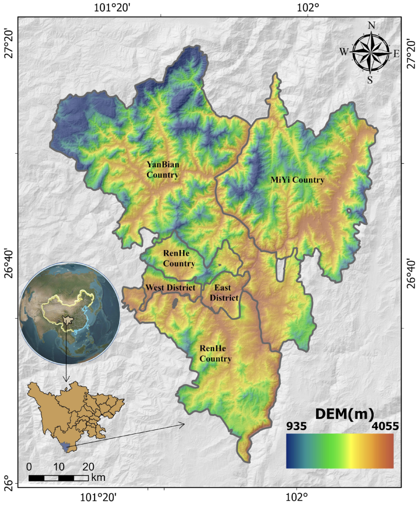
2.1. Study Area
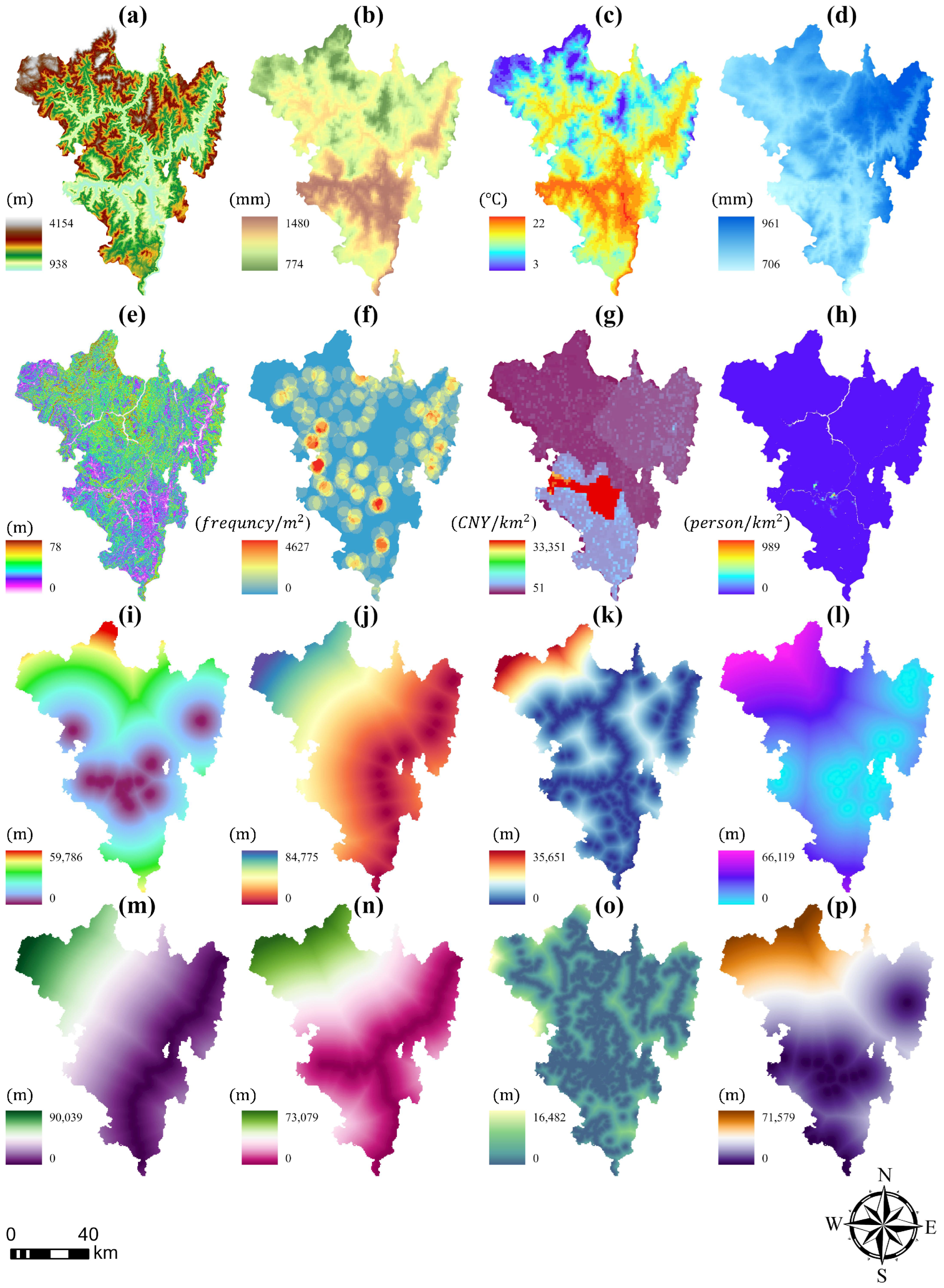
2.2. Data Sources
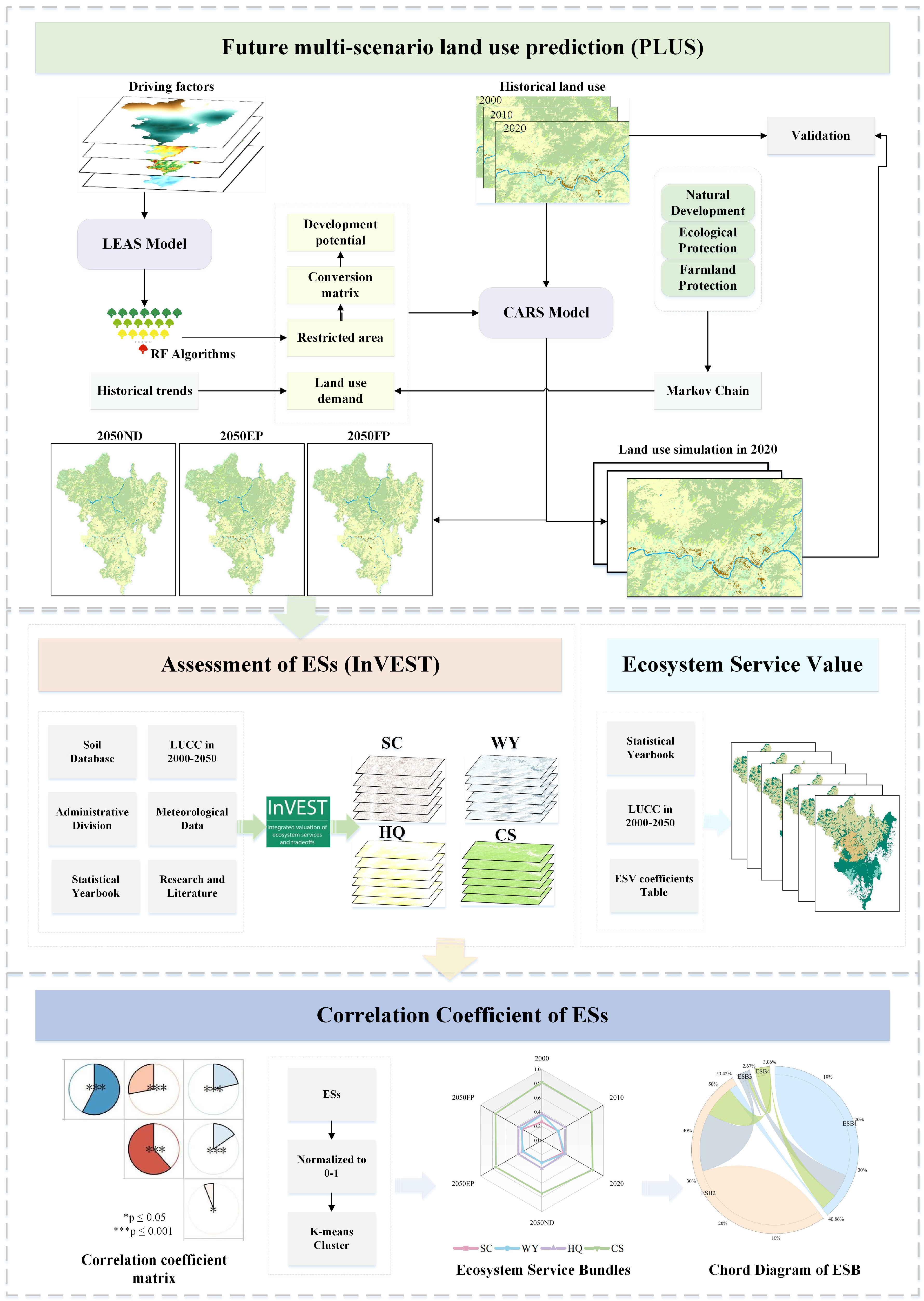
2.3. Methodology
2.3.1. Simulation of LULC across Multiple Scenarios
- (1)
- PLUS Model
- (2)
- Multi-scenario Settings
- (3)
- Model Validation
2.3.2. Evaluation of Ecosystem Services (InVEST)
- (1)
- Soil Conservation (SC)
- (2)
- Water Yield (WY)
- (3)
- Habitat Quality (HQ)
- (4)
- Carbon Storage (CS)
2.3.3. Valuation of Ecosystem Service Value (ESV)
2.3.4. Statistical Analysis
- (1)
- Analysis of Correlation
- (2)
- Identification of Ecosystem Service Bundles
3. Results
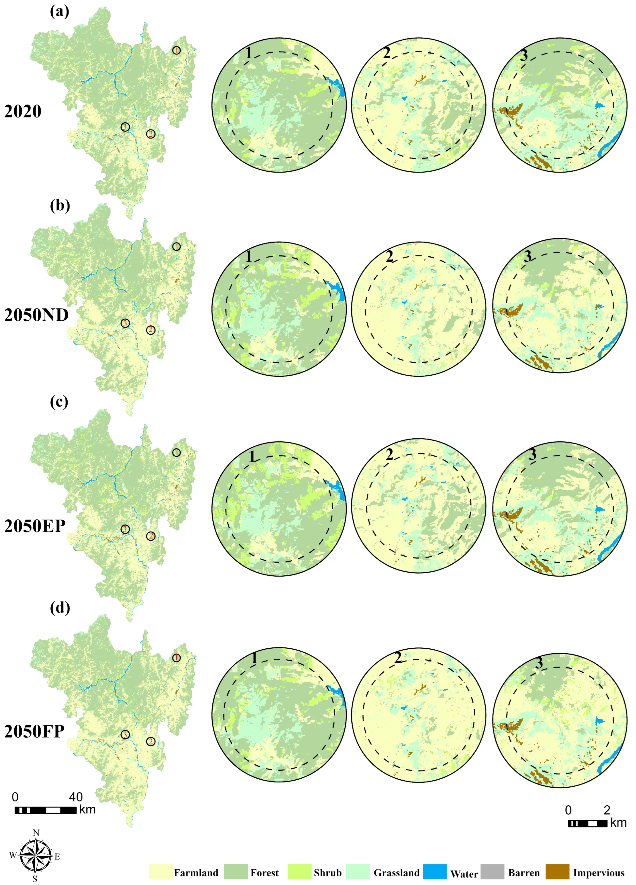
3.1. LULC from 2000 to 2050
3.2. Analysis of Changes in ESs and ESV
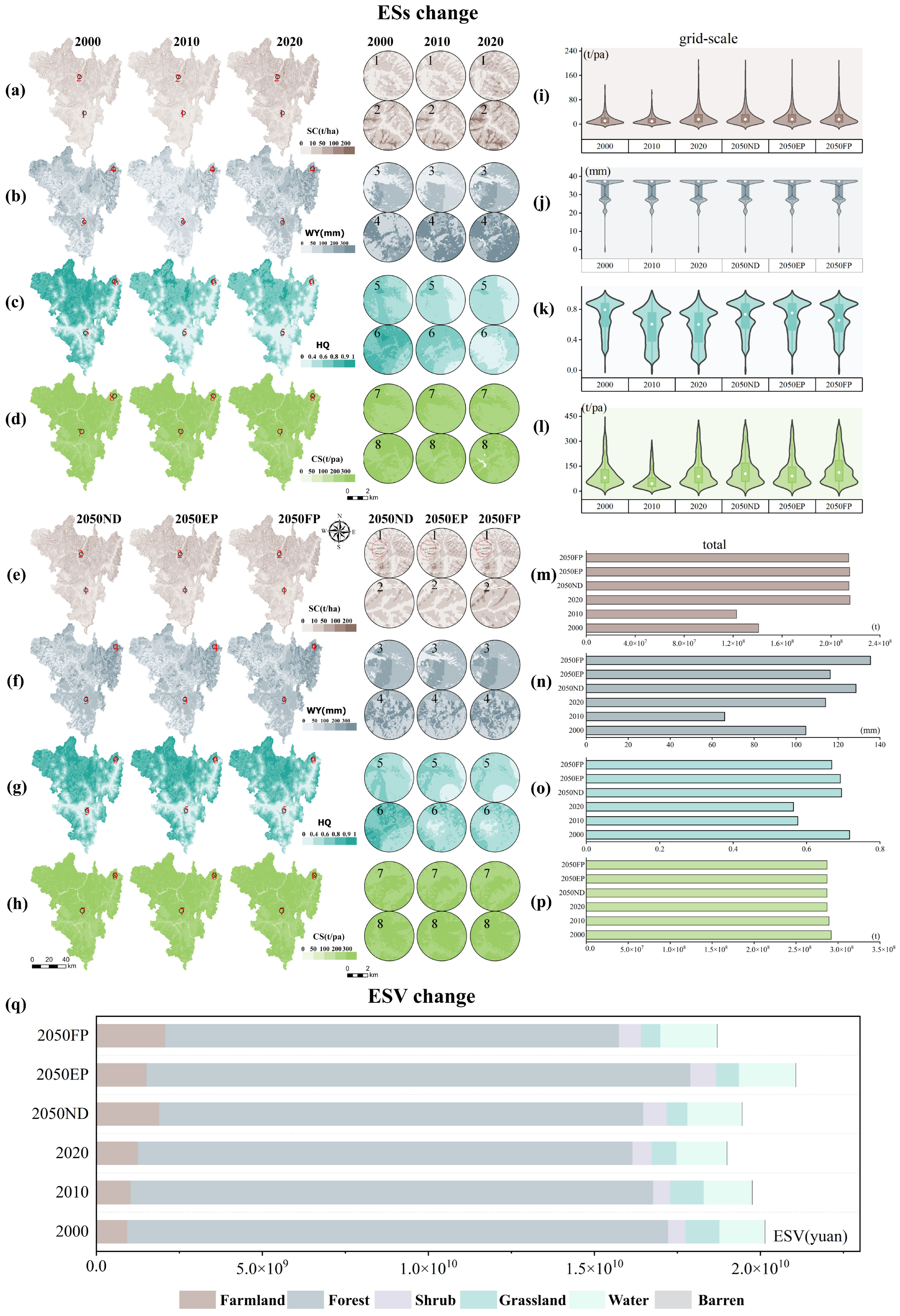
3.2.1. ESs Changes
3.2.2. ESV Changes
3.3. Trade-Offs, Synergies, and Bundling of ESs
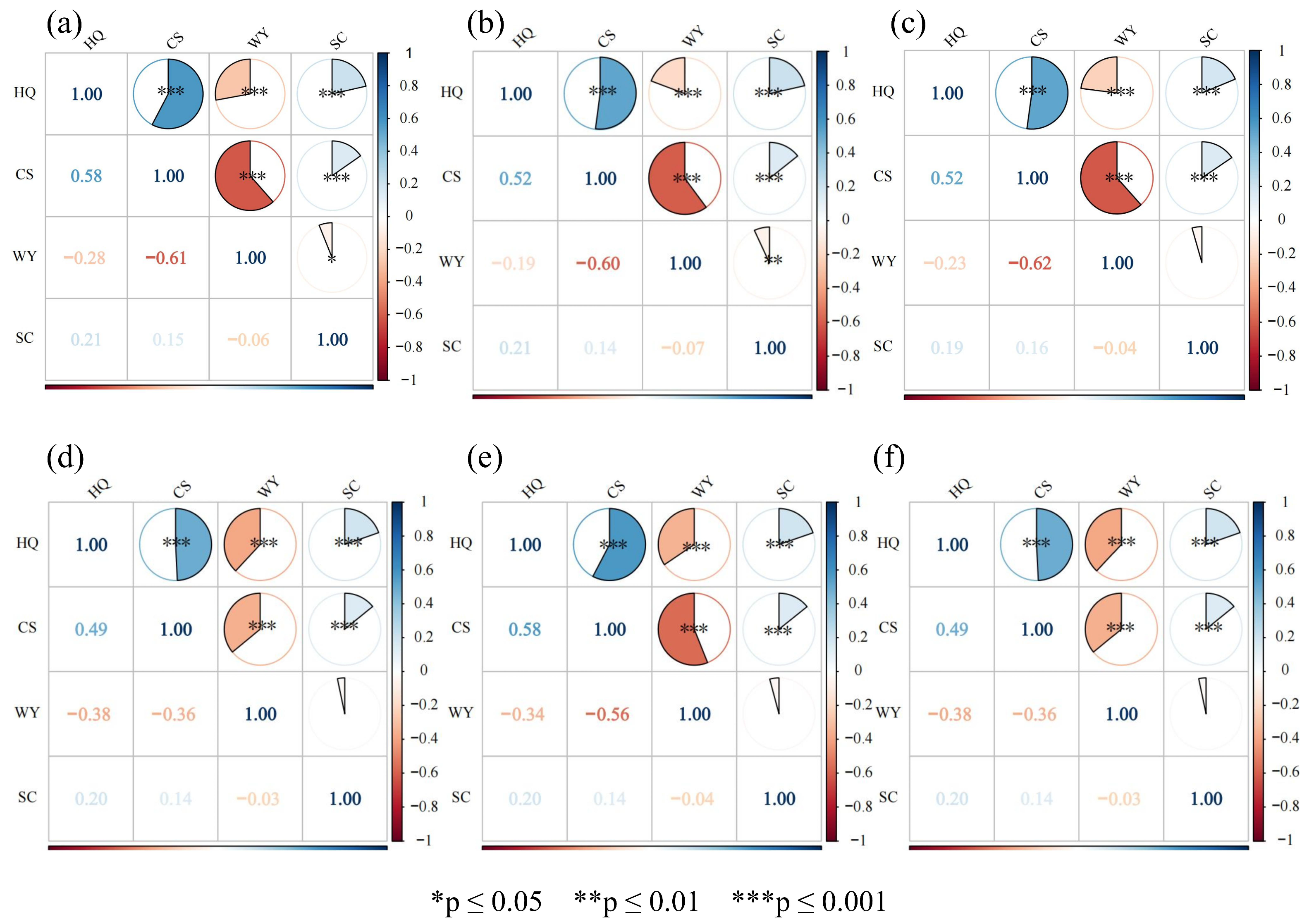
3.3.1. Trade-Offs and Synergies among ESs during 2000–2050
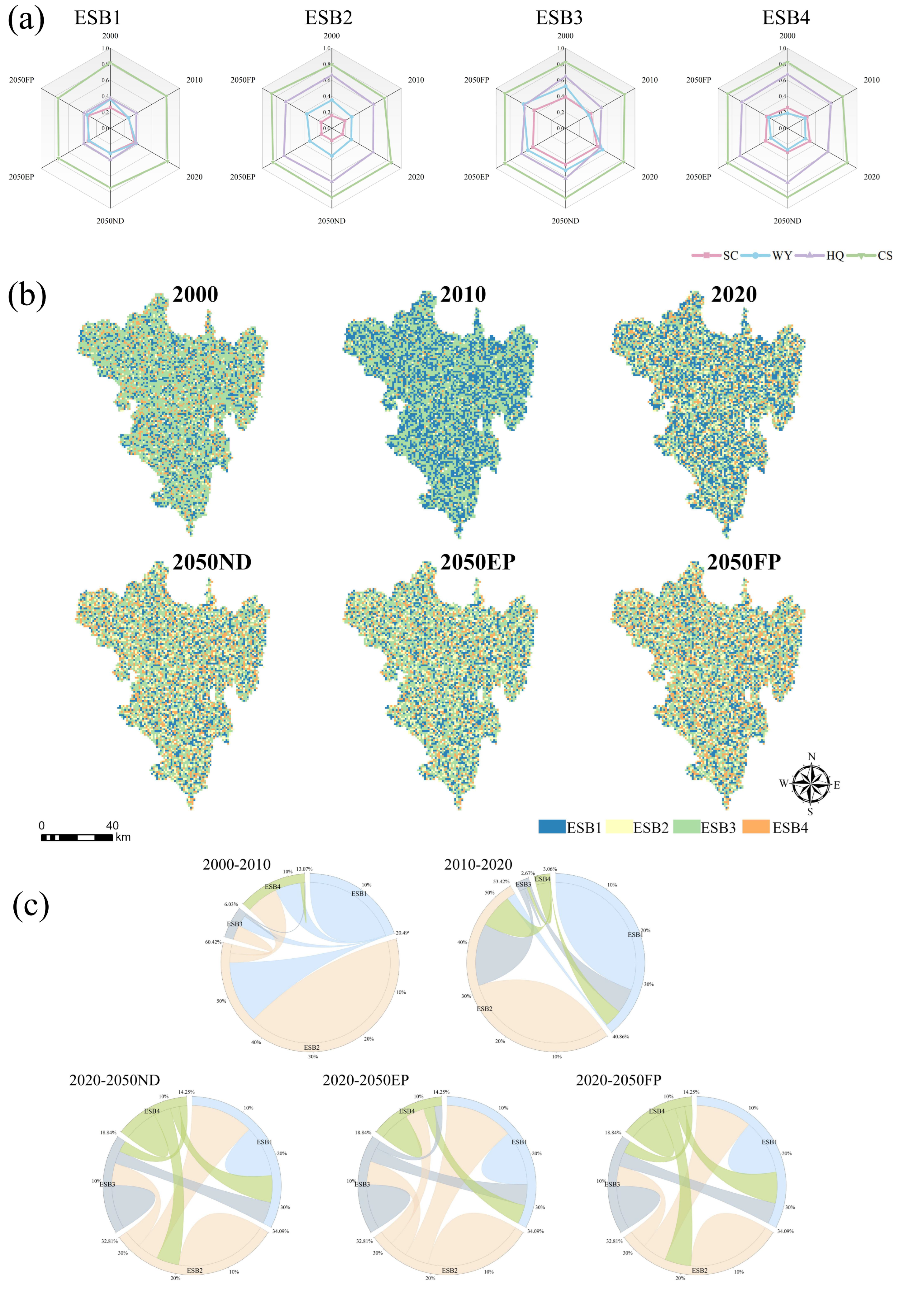
3.3.2. Spatiotemporal Distribution of ESBs during 2000–2050
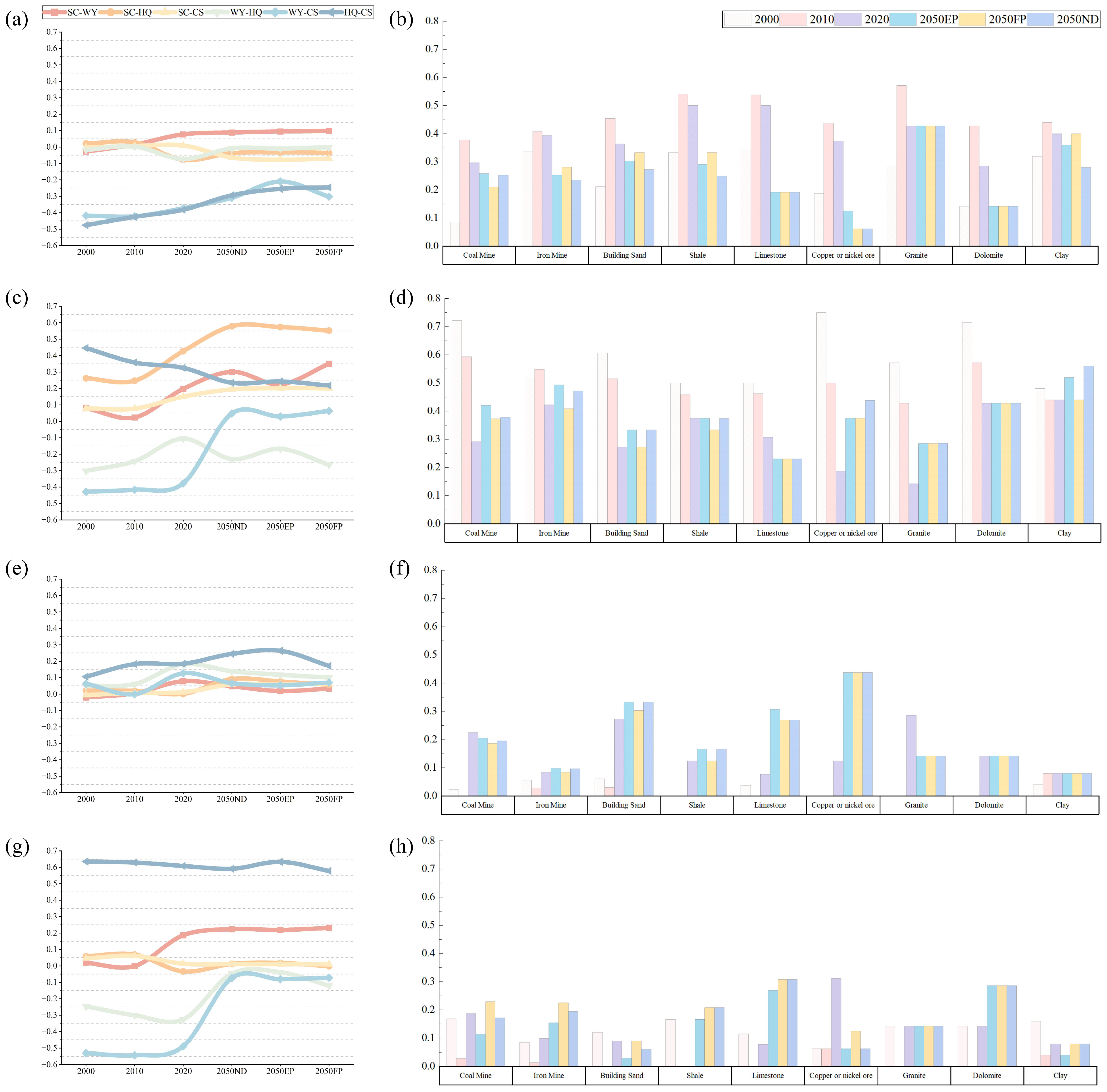
3.4. Changes in Interactions among Mining Ecosystem Services
4. Discussion
4.1. Significance and Valuation of the ESVs
4.2. Impacts of LULC on ESs
4.3. Multiple ES Interactions: Trade-Offs and Synergies across Various ESBs
4.4. Investigating Variations in Interactions among Mining ESs Based on Mineral Type
4.5. Limitations and Prospects
5. Conclusions
Author Contributions
Funding
Data Availability Statement
Conflicts of Interest
Appendix A

| Primary Categorization | Secondary Categorization | Farmland | Forest | Shrub | Grassland | Water | Barren |
|---|---|---|---|---|---|---|---|
| Provisioning services | Supply of food | 1702.99 | 421.25 | 292.82 | 359.61 | 1232.94 | 0 |
| Raw ingredient | 377.59 | 970.94 | 662.7 | 529.14 | 354.47 | 0 | |
| Provision of water | −2011.23 | 503.45 | 339.06 | 292.82 | 12,776.31 | 0 | |
| Regulating services | Regulation of gas | 1371.64 | 3195.36 | 2173.05 | 1859.68 | 1186.7 | 30.82 |
| Regulation of climate | 716.64 | 9555.26 | 6519.15 | 4916.33 | 3529.28 | 0 | |
| Cleanse the environment | 208.06 | 2779.24 | 1972.7 | 1623.37 | 8553.5 | 154.12 | |
| Hydrological Regulation | 2304.05 | 5954.06 | 5162.92 | 3601.2 | 157,569.3 | 46.24 | |
| Supporting services | Formation and preservation of soil | 801.41 | 3888.89 | 2650.81 | 2265.52 | 1433.29 | 30.82 |
| Maintaining nutrient cycling | 238.88 | 297.96 | 200.35 | 174.67 | 107.88 | 0 | |
| Conservation of biodiversity | 262 | 3539.56 | 2419.64 | 2060.03 | 3929.99 | 30.82 | |
| Cultural services | Entertainment and Culture | 115.59 | 1551.45 | 1063.41 | 909.29 | 2912.81 | 15.41 |
References
- Costanza, R.; d’Arge, R.; de Groot, R.; Farber, S.; Grasso, M.; Hannon, B.; Limburg, K.; Naeem, S.; O’Neill, R.V.; Paruelo, J.; et al. The value of the world’s ecosystem services and natural capital. Ecol. Econ. 1998, 25, 3–15. [Google Scholar] [CrossRef]
- Daily, G.; Postel, S.; Bawa, K.; Kaufman, L. Nature’s Services: Societal Dependence On Natural Ecosystems; Island Press: Chicago, IL, USA, 1997; pp. 1–10. [Google Scholar]
- Kareiva, P.; Watts, S.; McDonald, R.; Boucher, T. Domesticated nature: Shaping landscapes and ecosystems for human welfare. Science 2007, 316, 1866–1869. [Google Scholar] [CrossRef] [PubMed]
- Xie, G.; Zhang, C.; Zhang, C.; Xiao, Y.; Lu, C. The value of ecosystem services in China. Resour. Sci. 2015, 37, 1740–1746. [Google Scholar]
- Jopke, C.; Kreyling, J.; Maes, J.; Koellner, T. Interactions among ecosystem services across Europe: Bagplots and cumulative correlation coefficients reveal synergies, trade-offs, and regional patterns. Ecol. Indic. 2015, 49, 46–52. [Google Scholar] [CrossRef]
- Cord, A.F.; Bartkowski, B.; Beckmann, M.; Dittrich, A.; Hermans-Neumann, K.; Kaim, A.; Lienhoop, N.; Locher-Krause, K.; Priess, J.; Schroeter-Schlaack, C.; et al. Towards systematic analyses of ecosystem service trade-offs and synergies: Main concepts, methods and the road ahead. Ecosyst. Serv. 2017, 28, 264–272. [Google Scholar] [CrossRef]
- Bradford, J.B.; D’Amato, A.W. Recognizing trade-offs in multi-objective land management. Front. Ecol. Environ. 2012, 10, 210–216. [Google Scholar] [CrossRef] [PubMed]
- Lin, S.; Wu, R.; Yang, F.; Wang, J.; Wu, W. Spatial trade-offs and synergies among ecosystem services within a global biodiversity hotspot. Ecol. Indic. 2018, 84, 371–381. [Google Scholar] [CrossRef]
- Rodriguez, J.P.; Beard, T.; Douglas, J.; Bennett, E.M.; Cumming, G.S.; Cork, S.J.; Agard, J.; Dobson, A.P.; Peterson, G.D. Trade-offs across space, time, and ecosystem services. Ecol. Soc. 2006, 11, 28. [Google Scholar] [CrossRef]
- Zhang, Z.; Liu, Y.; Zhang, Y.; Liu, Y.; Lu, Y.; Ren, Q. Spatial Non-Stationary Response of the Ecosystem Services Synergy and Tradeoff to Influencing Factors:A Case Study of Ecological Function Area in Fujian Province. Geomat. Inf. Sci. Wuhan Univ. 2022, 47, 111–125. [Google Scholar] [CrossRef]
- Raudsepp-Hearne, C.; Peterson, G.D.; Bennett, E.M. Ecosystem service bundles for analyzing tradeoffs in diverse landscapes. Proc. Natl. Acad. Sci. USA 2010, 107, 5242–5247. [Google Scholar] [CrossRef]
- Spake, R.; Lasseur, R.; Crouzat, E.; Bullock, J.M.; Lavorel, S.; Parks, K.E.; Schaafsma, M.; Bennett, E.M.; Maes, J.; Mulligan, M.; et al. Unpacking ecosystem service bundles: Towards predictive mapping of synergies and trade-offs between ecosystem services. Glob. Environ. Change-Human Policy Dimens. 2017, 47, 37–50. [Google Scholar] [CrossRef]
- Agudelo, C.A.R.; Bustos, S.L.H.; Moreno, C.A.P. Modeling interactions among multiple ecosystem services. A critical review. Ecol. Model. 2020, 429, 109103. [Google Scholar] [CrossRef]
- Turner, K.G.; Odgaard, M.V.; Bocher, P.K.; Dalgaard, T.; Svenning, J.C. Bundling ecosystem services in Denmark: Trade-offs and synergies in a cultural landscape. Landsc. Urban Plan. 2014, 125, 89–104. [Google Scholar] [CrossRef]
- Yang, H.; Zhong, X.; Deng, S.; Xu, H. Assessment of the impact of LUCC on NPP and its influencing factors in the Yangtze River basin, China. Catena 2021, 206, 105542. [Google Scholar] [CrossRef]
- Xiao, S.; Wu, W.; Guo, J.; Ou, M.; Pueppke, S.G.; Ou, W.; Tao, Y. An evaluation framework for designing ecological security patterns and prioritizing ecological corridors: Application in Jiangsu Province, China. Landsc. Ecol. 2020, 35, 2517–2534. [Google Scholar] [CrossRef]
- Bhatta, B.; Shrestha, S.; Shrestha, P.K.; Talchabhadel, R. Evaluation and application of a SWAT model to assess the climate change impact on the hydrology of the Himalayan River Basin. Catena 2019, 181, 104082. [Google Scholar] [CrossRef]
- Abbaspour, K.C.; Rouholahnejad, E.; Vaghefi, S.; Srinivasan, R.; Yang, H.; Klove, B. A continental-scale hydrology and water quality model for Europe: Calibration and uncertainty of a high-resolution large-scale SWAT model. J. Hydrol. 2015, 524, 733–752. [Google Scholar] [CrossRef]
- Zhang, K.; Tang, X.; Zhao, Y.; Huang, B.; Huang, L.; Liu, M.; Luo, E.; Li, Y.; Jiang, T.; Zhang, L.; et al. Differing perceptions of the youth and the elderly regarding cultural ecosystem services in urban parks: An exploration of the tour experience. Sci. Total Environ. 2022, 821, 153388. [Google Scholar] [CrossRef] [PubMed]
- Nelson, E.; Mendoza, G.; Regetz, J.; Polasky, S.; Tallis, H.; Cameron, D.R.; Chan, K.M.A.; Daily, G.C.; Goldstein, J.; Kareiva, P.M.; et al. Modeling multiple ecosystem services, biodiversity conservation, commodity production, and tradeoffs at landscape scales. Front. Ecol. Environ. 2009, 7, 4–11. [Google Scholar] [CrossRef]
- Dittrich, A.; Seppelt, R.; Vaclavik, T.; Cord, A.F. Integrating ecosystem service bundles and socio-environmental conditions—A national scale analysis from Germany. Ecosyst. Serv. 2017, 28, 273–282. [Google Scholar] [CrossRef]
- Lyu, R.; Clarke, K.C.; Zhang, J.; Feng, J.; Jia, X.; Li, J. Spatial correlations among ecosystem services and their socio-ecological driving factors: A case study in the city belt along the Yellow River in Ningxia, China. Appl. Geogr. 2019, 108, 64–73. [Google Scholar] [CrossRef]
- Gao, J.; Yu, Z.; Wang, L.; Vejre, H. Suitability of regional development based on ecosystem service benefits and losses: A case study of the Yangtze River Delta urban agglomeration, China. Ecol. Indic. 2019, 107, 105579. [Google Scholar] [CrossRef]
- Gou, M.; Li, L.; Ouyang, S.; Wang, N.; La, L.; Liu, C.; Xiao, W. Identifying and analyzing ecosystem service bundles and their socioecological drivers in the Three Gorges Reservoir Area. J. Clean. Prod. 2021, 307, 127208. [Google Scholar] [CrossRef]
- Liu, Y.; Lu, Y.; Fu, B.; Harris, P.; Wu, L. Quantifying the spatio-temporal drivers of planned vegetation restoration on ecosystem services at a regional scale. Sci. Total Environ. 2019, 650, 1029–1040. [Google Scholar] [CrossRef] [PubMed]
- Queiroz, C.; Meacham, M.; Richter, K.; Norstrom, A.V.; Andersson, E.; Norberg, J.; Peterson, G. Mapping bundles of ecosystem services reveals distinct types of multifunctionality within a Swedish landscape. Ambio 2015, 44, S89–S101. [Google Scholar] [CrossRef] [PubMed]
- Zhang, Y.; Lu, X.; Liu, B.; Wu, D.; Fu, G.; Zhao, Y.; Sun, P. Spatial relationships between ecosystem services and socioecological drivers across a large-scale region: A case study in the Yellow River Basin. Sci. Total Environ. 2021, 766, 142480. [Google Scholar] [CrossRef]
- Orsi, F.; Ciolli, M.; Primmer, E.; Varumo, L.; Geneletti, D. Mapping hotspots and bundles of forest ecosystem services across the European Union. Land Use Pol. 2020, 99, 104840. [Google Scholar] [CrossRef]
- Hsieh, C.H.; Lin, H.W.; Liu, W.Y. Assessing the ecosystem services provided by conventional and organic farmlands: A better outcome for organic farmlands? Ecosyst. Serv. 2023, 60, 101514. [Google Scholar] [CrossRef]
- Li, S.; Zhao, Y.; Xiao, W.; Yellishetty, M.; Yang, D. Identifying ecosystem service bundles and the spatiotemporal characteristics of trade-offs and synergies in coal mining areas with a high groundwater table. Sci. Total Environ. 2022, 807, 151036. [Google Scholar] [CrossRef]
- Liu, J.; Pei, X.; Zhu, W.; Jiao, J. Scenario modeling of ecosystem service trade-offs and bundles in a semi-arid valley basin. Sci. Total Environ. 2023, 896, 166413. [Google Scholar] [CrossRef]
- Paudel, S.; States, S.L. Urban green spaces and sustainability: Exploring the ecosystem services and disservices of grassy lawns versus floral meadows. Urban For. Urban Green. 2023, 84, 127932. [Google Scholar] [CrossRef]
- Hasan, S.S.; Zhen, L.; Miah, M.G.; Ahamed, T.; Samie, A. Impact of land use change on ecosystem services: A review. Environ. Dev. 2020, 34, 100527. [Google Scholar] [CrossRef]
- Liu, Y.; Tong, Z.; Liu, S.; Huang, D. Progress and Prospects of Research on Optimal Land-Use Allocation Modeling. Geomat. Inf. Sci. Wuhan Univ. 2022, 47, 1598–1614. [Google Scholar] [CrossRef]
- Tolessa, T.; Senbeta, F.; Kidane, M. The impact of land use/land cover change on ecosystem services in the central highlands of Ethiopia. Ecosyst. Serv. 2017, 23, 47–54. [Google Scholar] [CrossRef]
- Zhang, M.; Dai, Z.; Bouma, T.J.; Bricker, J.; Townend, I.; Wen, J.; Zhao, T.; Cai, H. Tidal-flat reclamation aggravates potential risk from storm impacts. Coast. Eng. 2021, 166, 103868. [Google Scholar] [CrossRef]
- Wang, Z.; Li, X.; Mao, Y.; Li, L.; Wang, X.; Lin, Q. Dynamic simulation of land use change and assessment of carbon storage based on climate change scenarios at the city level: A case study of Bortala, China. Ecol. Indic. 2022, 134, 108499. [Google Scholar] [CrossRef]
- Zhang, Y.; Li, Y.; Lv, J.; Wang, J.; Wu, Y. Scenario simulation of ecological risk based on land use/cover change-A case study of the Jinghe county, China. Ecol. Indic. 2021, 131, 108176. [Google Scholar] [CrossRef]
- Li, X.; Chen, G.; Liu, X.; Liang, X.; Wang, S.; Chen, Y.; Pei, F.; Xu, X. A New Global Land-Use and Land-Cover Change Product at a 1-km Resolution for 2010 to 2100 Based on Human-Environment Interactions. Ann. Am. Assoc. Geogr. 2017, 107, 1040–1059. [Google Scholar] [CrossRef]
- Liu, X.; Liang, X.; Li, X.; Xu, X.; Ou, J.; Chen, Y.; Li, S.; Wang, S.; Pei, F. A future land use simulation model (FLUS) for simulating multiple land use scenarios by coupling human and natural effects. Landsc. Urban Plan. 2017, 168, 94–116. [Google Scholar] [CrossRef]
- Wang, H.; Stephenson, S.R.; Qu, S. Modeling spatially non-stationary land use/cover change in the lower Connecticut River Basin by combining geographically weighted logistic regression and the CA-Markov model. Int. J. Geogr. Inf. Sci. 2019, 33, 1313–1334. [Google Scholar] [CrossRef]
- Su, Y.; Ma, X.; Feng, Q.; Liu, W.; Zhu, M.; Niu, J.; Liu, G.; Shi, L. Patterns and controls of ecosystem service values under different land-use change scenarios in a mining-dominated basin of northern China. Ecol. Indic. 2023, 151, 110321. [Google Scholar] [CrossRef]
- Liang, X.; Guan, Q.; Clarke, K.C.; Liu, S.; Wang, B.; Yao, Y. Understanding the drivers of sustainable land expansion using a patch-generating land use simulation (PLUS) model: A case study in Wuhan, China. Comput. Environ. Urban Syst. 2021, 85, 101569. [Google Scholar] [CrossRef]
- Gaur, S.; Singh, R. A Comprehensive Review on Land Use/Land Cover (LULC) Change Modeling for Urban Development: Current Status and Future Prospects. Sustainability 2023, 15, 903. [Google Scholar] [CrossRef]
- Magliocca, N.R.; Dhungana, P.; Sink, C.D. Review of counterfactual land change modeling for causal inference in land system science. J. Land Use Sci. 2023, 18, 1–24. [Google Scholar] [CrossRef]
- Ericsson, M.; Löf, O. Mining’s contribution to national economies between 1996 and 2016. Miner. Econ. 2019, 32, 223–250. [Google Scholar] [CrossRef]
- Kumi, S.; Addo-Fordjour, P.; Fei-Baffoe, B. Mining-induced changes in ecosystem services value and implications of their economic and relational cost in a mining landscape, Ghana. Heliyon 2023, 9, e21156. [Google Scholar] [CrossRef] [PubMed]
- Castello, L.; Macedo, M.N. Large-scale degradation of Amazonian freshwater ecosystems. Glob. Chang. Biol. 2016, 22, 990–1007. [Google Scholar] [CrossRef]
- Boldy, R.; Santini, T.; Annandale, M.; Erskine, P.D.; Sonter, L.J. Understanding the impacts of mining on ecosystem services through a systematic review. Extr. Ind. Soc. 2021, 8, 457–466. [Google Scholar] [CrossRef]
- Sonter, L.J.; Herrera, D.; Barrett, D.J.; Galford, G.L.; Moran, C.J.; Soares-Filho, B.S. Mining drives extensive deforestation in the Brazilian Amazon. Nat. Commun. 2017, 8, 1013. [Google Scholar] [CrossRef]
- Zhang, M.; Schwarz, C.; Lin, W.; Naing, H.; Cai, H.; Zhu, Z. A new perspective on the impacts of Spartina alterniflora invasion on Chinese wetlands in the context of climate change: A case study of the Jiuduansha Shoals, Yangtze Estuary. Sci. Total Environ. 2023, 868, 161477. [Google Scholar] [CrossRef]
- Xiang, H.; Wang, Z.; Mao, D.; Zhang, J.; Zhao, D.; Zeng, Y.; Wu, B. Surface mining caused multiple ecosystem service losses in China. J. Environ. Manag. 2021, 290, 112618. [Google Scholar] [CrossRef] [PubMed]
- Jiao, W.; Zhang, X.; Li, C.; Guo, J. Sustainable transition of mining cities in China: Literature review and policy analysis. Resour. Policy 2021, 74, 101867. [Google Scholar] [CrossRef]
- Wang, Z.; Lechner, A.M.; Yang, Y.; Baumgartl, T.; Wu, J. Mapping the cumulative impacts of long-term mining disturbance and progressive rehabilitation on ecosystem services. Sci. Total Environ. 2020, 717, 137214. [Google Scholar] [CrossRef] [PubMed]
- Li, L.; Lei, Y.; Wu, S.; He, C.; Yan, D. Study on the coordinated development of economy, environment and resource in coal-based areas in Shanxi Province in China: Based on the multi-objective optimization model. Resour. Policy 2018, 55, 80–86. [Google Scholar] [CrossRef]
- Wen, B.; Pan, Y.; Zhang, Y.; Liu, J.; Xia, M. Does the Exhaustion of Resources Drive Land Use Changes? Evidence from the Influence of Coal Resources-Exhaustion on Coal Resources-Based Industry Land Use Changes. Sustainability 2018, 10, 2698. [Google Scholar] [CrossRef]
- Dai, X.; Gao, Y.; He, X.; Liu, T.; Jiang, B.; Shao, H.; Yao, Y. Spatial-temporal pattern evolution and driving force analysis of ecological environment vulnerability in Panzhihua City. Environ. Sci. Pollut. Res. 2021, 28, 7151–7166. [Google Scholar] [CrossRef] [PubMed]
- Peng, S. 1 km Monthly Potential Evapotranspiration Dataset in China (1901–2022); National Tibetan Plateau Data Center: Beijing, China, 2022. [Google Scholar] [CrossRef]
- Du, S.; Zhou, Z.; Huang, D.; Zhang, F.; Deng, F.; Yang, Y. The Response of Carbon Stocks to Land Use/Cover Change and a Vulnerability Multi-Scenario Analysis of the Karst Region in Southern China Based on PLUS-InVEST. Forests 2023, 14, 2307. [Google Scholar] [CrossRef]
- Xu, C.; Zhang, Q.; Yu, Q.; Wang, J.; Wang, F.; Qiu, S.; Ai, M.; Zhao, J. Effects of land use/cover change on carbon storage between 2000 and 2040 in the Yellow River Basin, China. Ecol. Indic. 2023, 151, 110345. [Google Scholar] [CrossRef]
- Varga, O.G.; Pontius, R.; Gilmore, J.; Singh, S.K.; Szabo, S. Intensity Analysis and the Figure of Merit’s components for assessment of a Cellular Automata - Markov simulation model. Ecol. Indic. 2019, 101, 933–942. [Google Scholar] [CrossRef]
- Deng, Z.; Quan, B.; Zhang, H.; Xie, H.; Zhou, Z. Scenario Simulation of Land Use and Cover under Safeguarding Ecological Security: A Case Study of Chang-Zhu-Tan Metropolitan Area, China. Forests 2023, 14, 2131. [Google Scholar] [CrossRef]
- Bai, Y.; Ochuodho, T.O.; Yang, J. Impact of land use and climate change on water-related ecosystem services in Kentucky, USA. Ecol. Indic. 2019, 102, 51–64. [Google Scholar] [CrossRef]
- Gao, J.; Li, F.; Gao, H.; Zhou, C.; Zhang, X. The impact of land-use change on water-related ecosystem services: A study of the Guishui River Basin, Beijing, China. J. Clean. Prod. 2017, 163, S148–S155. [Google Scholar] [CrossRef]
- Yohannes, H.; Soromessa, T.; Argaw, M.; Dewan, A. Impact of landscape pattern changes on hydrological ecosystem services in the Beressa watershed of the Blue Nile Basin in Ethiopia. Sci. Total Environ. 2021, 793, 148559. [Google Scholar] [CrossRef] [PubMed]
- Aneseyee, A.B.; Noszczyk, T.; Soromessa, T.; Elias, E. The InVEST Habitat Quality Model Associated with Land Use/Cover Changes: A Qualitative Case Study of the Winike Watershed in the Omo-Gibe Basin, Southwest Ethiopia. Remote Sens. 2020, 12, 1103. [Google Scholar] [CrossRef]
- Wu, L.; Sun, C.; Fan, F. Estimating the Characteristic Spatiotemporal Variation in Habitat Quality Using the InVEST Model-A Case Study from Guangdong-Hong Kong-Macao Greater Bay Area. Remote Sens. 2021, 13, 1008. [Google Scholar] [CrossRef]
- Fu, B.; Xu, P.; Wang, Y.; Guo, Y. Integrating Ecosystem Services and Human Demand for a New Ecosystem Management Approach: A Case Study from the Giant Panda World Heritage Site. Sustainability 2020, 12, 295. [Google Scholar] [CrossRef]
- Xie, X.; Zhu, Q. Research on the Impact of Urban Expansion on Habitat Quality in Chengdu. Sustainability 2023, 15, 6271. [Google Scholar] [CrossRef]
- Babbar, D.; Areendran, G.; Sahana, M.; Sarma, K.; Raj, K.; Sivadas, A. Assessment and prediction of carbon sequestration using Markov chain and InVEST model in Sariska Tiger Reserve, India. J. Clean. Prod. 2021, 278, 123333. [Google Scholar] [CrossRef]
- Liu, Q.; Yang, D.; Cao, L.; Anderson, B. Assessment and Prediction of Carbon Storage Based on Land Use/Land Cover Dynamics in the Tropics: A Case Study of Hainan Island, China. Land 2022, 11, 244. [Google Scholar] [CrossRef]
- Tian, L.; Tao, Y.; Fu, W.; Li, T.; Ren, F.; Li, M. Dynamic Simulation of Land Use/Cover Change and Assessment of Forest Ecosystem Carbon Storage under Climate Change Scenarios in Guangdong Province, China. Remote Sens. 2022, 14, 2330. [Google Scholar] [CrossRef]
- Xie, G.; Zhang, C.; Zhang, L.; Chen, W.; Li, S. Improvement of the Evaluation Method for Ecosystem Service Value Based on Per Unit Area. J. Nat. Resour. 2015, 30, 1243–1254. [Google Scholar] [CrossRef]
- Su, C.h.; Fu, B.J.; He, C.S.; Lü, Y.H. Variation of ecosystem services and human activities: A case study in the Yanhe Watershed of China. Acta Oecol. Int. J. Ecol. 2012, 44, 46–57. [Google Scholar] [CrossRef]
- Zeng, J.; Xu, J.; Li, W.; Dai, X.; Zhou, J.; Shan, Y.; Zhang, J.; Li, W.; Lu, H.; Ye, Y.; et al. Evaluating Trade-Off and Synergies of Ecosystem Services Values of a Representative Resources-Based Urban Ecosystem: A Coupled Modeling Framework Applied to Panzhihua City, China. Remote Sens. 2022, 14, 5282. [Google Scholar] [CrossRef]
- Gao, X.J.; Gray, J.M.; Reich, B.J. Long-term, medium spatial resolution annual land surface phenology with a Bayesian hierarchical model. Remote Sens. Environ. 2021, 261, 112484. [Google Scholar] [CrossRef]
- Zhang, J.; Li, S.; Lin, N.; Lin, Y.; Yuan, S.; Zhang, L.; Zhu, J.; Wang, K.; Gan, M.; Zhu, C. Spatial identification and trade-off analysis of land use functions improve spatial zoning management in rapid urbanized areas, China. Land Use Pol. 2022, 116, 106058. [Google Scholar] [CrossRef]
- Dai, X.; Fan, W.; Shan, Y.; Gao, Y.; Liu, C.; Nie, R.; Zhang, D.; Li, W.; Zhang, L.; Sun, X.; et al. LAI-Based Phenological Changes and Climate Sensitivity Analysis in the Three-River Headwaters Region. Remote Sens. 2022, 14, 3748. [Google Scholar] [CrossRef]
- Wu, L.; Sun, C.; Fan, F. Multi-criteria framework for identifying the trade-offs and synergies relationship of ecosystem services based on ecosystem services bundles. Ecol. Indic. 2022, 144, 109453. [Google Scholar] [CrossRef]
- Zhang, T.; Zhang, S.; Cao, Q.; Wang, H.; Li, Y. The spatiotemporal dynamics of ecosystem services bundles and the social-economic-ecological drivers in the Yellow River Delta region. Ecol. Indic. 2022, 135, 108573. [Google Scholar] [CrossRef]
- Daily, G.C.; Söderqvist, T.; Aniyar, S.; Arrow, K.; Dasgupta, P.; Ehrlich, P.R.; Folke, C.; Jansson, A.; Jansson, B.O.; Kautsky, N.; et al. Ecology. The value of nature and the nature of value. Science 2000, 289, 395–396. [Google Scholar] [CrossRef]
- Egoh, B.; Rouget, M.; Reyers, B.; Knight, A.T.; Cowling, R.M.; van Jaarsveld, A.S.; Welz, A. Integrating ecosystem services into conservation assessments: A review. Ecol. Econ. 2007, 63, 714–721. [Google Scholar] [CrossRef]
- Peng, K.; Jiang, W.; Ling, Z.; Hou, P.; Deng, Y. Evaluating the potential impacts of land use changes on ecosystem service value under multiple scenarios in support of SDG reporting: A case study of the Wuhan urban agglomeration. J. Clean. Prod. 2021, 307. [Google Scholar] [CrossRef]
- Xie, G.; Lin, Z.; Chun-xia, L.U.; Yu, X.; Cao, C. Expert Knowledge Based Valuation Method of Ecosystem Services in China. J. Nat. Resour. 2008, 23, 911–919. [Google Scholar] [CrossRef]
- Ge, G.; Zhang, J.; Chen, X.; Liu, X.; Hao, Y.; Yang, X.; Kwon, S. Effects of land use and land cover change on ecosystem services in an arid desert-oasis ecotone along the Yellow River of China. Ecol. Eng. 2022, 176, 106512. [Google Scholar] [CrossRef]
- He, C.; Shao, H.; Xian, W. Spatiotemporal Variation and Driving Forces Analysis of Eco-System Service Values: A Case Study of Sichuan Province, China. Int. J. Environ. Res. Public Health 2022, 19, 8595. [Google Scholar] [CrossRef] [PubMed]
- Tan, Z.; Guan, Q.; Lin, J.; Yang, L.; Luo, H.; Ma, Y.; Tian, J.; Wang, Q.; Wang, N. The response and simulation of ecosystem services value to land use/land cover in an oasis, Northwest China. Ecol. Indic. 2020, 118, 106711. [Google Scholar] [CrossRef]
- Schaaf, W.; Pohle, I.; Maurer, T.; Gerwin, W.; Hinz, C.; Badorreck, A. Water balance dynamics during ten years of ecological development at Chicken Creek catchment. Vadose Zone J. 2017, 16, 1–14. [Google Scholar] [CrossRef]
- Zaplata, M.K.; Winter, S.; Fischer, A.; Kollmann, J.; Ulrich, W. Species-driven phases and increasing structure in early-successional plant communities. Am. Nat. 2013, 181, E17–E27. [Google Scholar] [CrossRef] [PubMed]
- Yuan, X.; Wang, C.; Li, B.; Wang, W.; Chen, N. Review of the Driving Forces and Impacts of Land Use/Cover Change in the Yangtze River Basin. Geomat. Inf. Sci. Wuhan Univ. 2023, 48, 1241–1255. [Google Scholar] [CrossRef]
- Shao, Z.; Chen, C.; Liu, Y.; Cao, J.; Liao, G.; Lin, Z. Impact of Land Use Change on Carbon Storage Based on FLUS-InVEST Model: A Case Study of Chengdu-Chongqing Urban Agglomeration, China. Land 2023, 12, 1531. [Google Scholar] [CrossRef]
- Li, X.; Liu, Z.; Li, S.; Li, Y. Multi-Scenario Simulation Analysis of Land Use Impacts on Habitat Quality in Tianjin Based on the PLUS Model Coupled with the InVEST Model. Sustainability 2022, 14, 6923. [Google Scholar] [CrossRef]
- Madani, E.M.; Jansson, P.E.; Babelon, I. Differences in water balance between grassland and forest watersheds using long-term data, derived using the CoupModel. Hydrol. Res. 2018, 49, 72–89. [Google Scholar] [CrossRef]
- Yang, D.; Liu, W.; Tang, L.; Chen, L.; Li, X.; Xu, X. Estimation of water provision service for monsoon catchments of South China: Applicability of the InVEST model. Landsc. Urban Plan. 2019, 182, 133–143. [Google Scholar] [CrossRef]
- Li, M.; Liang, D.; Xia, J.; Song, J.; Cheng, D.; Wu, J.; Cao, Y.; Sun, H.; Li, Q. Evaluation of water conservation function of Danjiang River Basin in Qinling Mountains, China based on InVEST model. J. Environ. Manag. 2021, 286, 112212. [Google Scholar] [CrossRef] [PubMed]
- Schaaf, W.; Hinz, C.; Gerwin, W.; Zaplata, M.K.; Huettl, R.F. Ecosystem development in the constructed catchment “chicken creek”. In Hydrology of Artificial and Controlled Experiments; Liu, J.F., Gu, W.Z., Eds.; Books on Demand: Norderstedt, Germany, 2018; pp. 75–93. [Google Scholar] [CrossRef]
- Yang, Y.; Li, M.; Feng, X.; Yan, H.; Su, M.; Wu, M. Spatiotemporal variation of essential ecosystem services and their trade-off/synergy along with rapid urbanization in the Lower Pearl River Basin, China. Ecol. Indic. 2021, 133, 108439. [Google Scholar] [CrossRef]
- Hu, X.; Ma, C.; Huang, P.; Guo, X. Ecological vulnerability assessment based on AHP-PSR method and analysis of its single parameter sensitivity and spatial autocorrelation for ecological protection: A case of Weifang City, China. Ecol. Indic. 2021, 125, 107464. [Google Scholar] [CrossRef]
- Vettegren, V.I.; Shcherbakov, I.P.; Voronin, A.V.; Kuksenko, V.S.; Mamalimov, R.I. Dynamics of the deformation and destruction of a heterogeneous body (granite) under the influence of an electric discharge. Phys. Solid State 2014, 56, 1018–1022. [Google Scholar] [CrossRef]
- Zaplata, M.K.; Dullau, S. Applying ecological succession theory to birds in solar parks: An approach to address protection and planning. Land 2022, 11, 718. [Google Scholar] [CrossRef]

| Data Name | Data Format | Data Sources |
|---|---|---|
| LULC data | https://zenodo.org/record/4417810#.YxhwS6HiviD (accessed on 24 September 2023) | |
| DEM data | Grids at 30 m resolution | https://www.gscloud.cn/search (accessed on 5 September 2023) |
| Precipitation data | ||
| Temperature data | https://www.geodata.cn (accessed on 17 September 2023) | |
| Evapotranspiration data | https://data.tpdc.ac.cn (accessed on 23 October 2023) [58] | |
| Soil type data | https://www.fao.org (accessed on 4 November 2023) | |
| GDP | ||
| Population density | Grids at 1 km resolution | https://www.resdc.cn/DOI (accessed on 25 October 2023) |
| Soil property dataset for land surface modeling across China | Grid at 30 arc-second resolution | http://poles.tpdc.ac.cn (accessed on 29 October 2023) |
| Secondary roads | ||
| Tertiary roads | ||
| Class IV roads | ||
| Motorways | ||
| Railways | ||
| High-speed rail stations | ||
| Government sites | ||
| Water bodies | https://www.webmap.cn/commres.do?method=result100W (accessed on 11 November 2023) | |
| Monitoring data from mining environments in Sichuan Province | Vector data | http://www.scddy.com.cn/ (accessed on 3 November 2023) |
| Panzhihua Statistical Yearbook | http://tjj.panzhihua.gov.cn/zwgk/tjsj/tjnj2022/index.shtml (accessed on 26 November 2023) | |
| China Yearbook of Agricultural Product Price Surveys | Text data | https://cnki.nbsti.net/CSYDMirror/Trade/home/index/Z009 (accessed on 2 December 2023) |
| r | 2000 | 2010 | 2020 | 2050ND | 2050EP | 2050FP | |
|---|---|---|---|---|---|---|---|
| ESB1 | SC-WY | −0.028 | 0.014 | 0.077 ** | 0.088 ** | 0.094 ** | 0.097 ** |
| SC-HQ | 0.021 | 0.028 | −0.078 ** | −0.038 * | −0.033 | −0.036 * | |
| SC-CS | −0.003 | 0.006 | 0.009 | −0.064 ** | −0.078 ** | −0.07** | |
| WY-HQ | −0.018 | 0.002 | −0.073 ** | −0.009 | −0.01 | −0.002 | |
| WY-CS | −0.418 ** | −0.422 ** | −0.373 ** | −0.309 ** | −0.210 ** | −0.302 ** | |
| HQ-CS | −0.476 ** | −0.425 ** | −0.382 ** | −0.294 ** | −0.255 ** | −0.246 ** | |
| ESB2 | SC-WY | 0.08 ** | 0.023 | 0.197 ** | 0.301 ** | 0.225 ** | 0.35 ** |
| SC-HQ | 0.262 ** | 0.247 ** | 0.427 ** | 0.579 ** | 0.574 ** | 0.552 ** | |
| SC-CS | 0.079 ** | 0.077 ** | 0.15 ** | 0.194 ** | 0.202 ** | 0.201 ** | |
| WY-HQ | −0.302 ** | −0.243 ** | −0.106 ** | −0.23 ** | −0.168 ** | −0.265 ** | |
| WY-CS | −0.429 ** | −0.417 ** | −0.378 ** | 0.047 ** | 0.029 | 0.063 ** | |
| HQ-CS | 0.446 ** | 0.358 ** | 0.325 ** | 0.234 ** | 0.242 ** | 0.218 ** | |
| ESB3 | SC-WY | −0.021 | 0.005 | 0.078 ** | 0.047 ** | 0.018 | 0.033 ** |
| SC-HQ | 0.021 | 0.019 | 0.001 | 0.091 ** | 0.076 ** | 0.056 ** | |
| SC-CS | −0.006 | 0.005 | 0.011 | 0.058 ** | 0.057 ** | 0.063 ** | |
| WY-HQ | 0.05 ** | 0.061 ** | 0.181 ** | 0.139 ** | 0.117 ** | 0.1 ** | |
| WY-CS | 0.063 ** | −0.001 | 0.126 * | 0.066 ** | 0.053 ** | 0.07 ** | |
| HQ-CS | 0.105 ** | 0.182 ** | 0.184 ** | 0.244 ** | 0.263 ** | 0.171 ** | |
| ESB4 | SC-WY | 0.018 | −0.001 | 0.186 ** | 0.223 ** | 0.218 ** | 0.231 ** |
| SC-HQ | 0.058 ** | 0.069 ** | −0.034 * | 0.012 | 0.017 | −0.002 | |
| SC-CS | 0.046 ** | 0.061 ** | 0.013 | 0.011 | 0.01 | 0.01 | |
| WY-HQ | −0.247 ** | −0.301 ** | −0.326 ** | −0.048 ** | −0.039 ** | −0.121** | |
| WY-CS | −0.531 * | −0.543 ** | −0.490 ** | −0.074 ** | −0.081 ** | −0.072** | |
| HQ-CS | 0.635 ** | 0.629 ** | 0.608 ** | 0.591 ** | 0.633 * | 0.578 ** | |
Disclaimer/Publisher’s Note: The statements, opinions and data contained in all publications are solely those of the individual author(s) and contributor(s) and not of MDPI and/or the editor(s). MDPI and/or the editor(s) disclaim responsibility for any injury to people or property resulting from any ideas, methods, instructions or products referred to in the content. |
© 2024 by the authors. Licensee MDPI, Basel, Switzerland. This article is an open access article distributed under the terms and conditions of the Creative Commons Attribution (CC BY) license (https://creativecommons.org/licenses/by/4.0/).
Share and Cite
Peng, X.; Dai, X.; Shi, R.; Zheng, Y.; Liu, X.; Xiao, Y.; Li, W.; Zhang, Y.; Wang, J.; Huang, H. Investigating the Effects of Mining on Ecosystem Services in Panzhihua City: A Multi-Scenario Analysis. Land 2024, 13, 819. https://doi.org/10.3390/land13060819
Peng X, Dai X, Shi R, Zheng Y, Liu X, Xiao Y, Li W, Zhang Y, Wang J, Huang H. Investigating the Effects of Mining on Ecosystem Services in Panzhihua City: A Multi-Scenario Analysis. Land. 2024; 13(6):819. https://doi.org/10.3390/land13060819
Chicago/Turabian StylePeng, Xuanmiao, Xiaoai Dai, Ryan Shi, Yujian Zheng, Xinyue Liu, Yuhe Xiao, Weile Li, Yang Zhang, Jue Wang, and Huan Huang. 2024. "Investigating the Effects of Mining on Ecosystem Services in Panzhihua City: A Multi-Scenario Analysis" Land 13, no. 6: 819. https://doi.org/10.3390/land13060819
APA StylePeng, X., Dai, X., Shi, R., Zheng, Y., Liu, X., Xiao, Y., Li, W., Zhang, Y., Wang, J., & Huang, H. (2024). Investigating the Effects of Mining on Ecosystem Services in Panzhihua City: A Multi-Scenario Analysis. Land, 13(6), 819. https://doi.org/10.3390/land13060819