Article

Effects of the Implementation Intensity of Ecological Engineering on Ecosystem Service Tradeoffs in Qinghai Province, China

1
Co-Innovation Center for Sustainable Forestry in Southern China, College of Ecology and Environment, Nanjing Forestry University, Nanjing 210037, China
2
Department of Forest and Conservation Sciences, University of British Columbia, Vancouver, BC V6T 1Z4, Canada
3
Northwest Surveying and Planning Institute of National Forestry and Grassland Administration, Key Laboratory National Forestry Administration on Ecological Hydrology and Disaster Prevention in Arid Regions, Xi’an 710048, China
4
College of Hydrology and Water Resources, Hohai University, Nanjing 210098, China
5
College of Forestry, Nanjing Forestry University, Nanjing 210037, China
6
College of Economics and Management, Nanjing Forestry University, Nanjing 210037, China
*
Authors to whom correspondence should be addressed.
Land 2024, 13(6), 848; https://doi.org/10.3390/land13060848
Submission received: 31 March 2024 / Revised: 7 June 2024 / Accepted: 8 June 2024 / Published: 14 June 2024
(This article belongs to the Section Land Environmental and Policy Impact Assessment)

Abstract

:
Ecological engineering (EE) has a profound impact on land-use dynamics, leading to alterations in ecosystem services (ESs). However, an appropriate EE implementation intensity that can balance the tradeoffs associated with altered ESs well has always been a concern for researchers and policymakers. In this study, we set the transition probability of farmland, bare land, and desertification land to forest and natural shrub, with 2010–2020 as the natural implementation scenario, as 10% for the low-intensity implementation scenario (LIS), 30% for the medium-intensity scenario, and 50% for the high-intensity scenario. The patch-generating land-use simulation (PLUS) model was used to project land-use patterns and the Integrated Valuation of Ecosystem Service and Tradeoffs (InVEST) model was used to simulate changes in the quality of ESs under four EE implementation intensities in 2030. We then performed a quantitative tradeoff analysis on the dominant ESs under four scenarios and used the production possibility frontier (PPF) curve to identify the optimal EE implementation intensity scenario. Our results indicated that an increase in EE implementation intensity would lead to an increase in soil retention, water purification, habitat quality, and carbon storage, but also to a decrease in water yield, aggravating the tradeoffs between water yield and other ESs. In all EE implementation intensity scenarios, the LIS had the lowest tradeoff intensity index and balanced ESs well, and thus was the optimal EE implementation scenario in Qinghai province. Our results provide knowledge to help decision makers select the appropriate EE intensity to maintain sustainable development. The integrated methodology can also be applied in other conservation regions to carry out practical land management.

1. Introduction

Ecosystem services (ESs), including various products and services derived from the structure and function of ecosystems, directly affect ecological security and human well-being [1,2]. Due to the heterogeneity of the spatial distribution of ecosystems and the complexity of ecological processes, the relationships among ESs mainly present as tradeoffs or synergies [3,4]. As the contradiction between the utilization of natural resources and ecological protection becomes more prominent, exploring the tradeoff relationships among different ESs is crucial for determining the maximum benefit of regional ecology and improving human well-being [5,6]. Land-use and land-cover (LULC) changes alter the main ecological functions and processes, leading to ES changes, which further significantly affects the ES tradeoffs [7]. Policy is one of the main driving forces of land-use change [8,9]. If the ES tradeoffs caused by land-use changes are not considered in policy-making, an effective balance between economic development and ecological and environmental protection cannot be achieved [10,11]. Therefore, clarifying the impact of policies on ESs and their tradeoffs is essential for regional ecosystem management.
To control the deterioration of ecosystems and promote the sustainable development of society, many policies related to ecological engineering (EE) have been carried out. Some countries and regions have implemented various large-scale projects for ecological restoration, such as the Thur and Töss rivers restoration projects in Switzerland [12], the US federal forest restoration programs on national forests [13], the ecological restoration of peatlands in Indonesia [14], the Mountain-River-Forest-Cropland-Lake-Grassland System Project [15], and the Natural Forest Protection Project (NFPP) [16] and Grain-for-Green Programme (GFGP) in China [17,18]. These ecological restoration projects are often accompanied by changes in land-use patterns, with an initial aim of improving one or more ESs [19]. As expected, EE has played an important role in increasing vegetation cover [20], controlling soil erosion [21], and improving habitats [22], achieving a remarkable effect in improving ecosystems from 2000 to 2020. However, the benefits of EE were often at the expense of reducing water yield (WY), especially in arid and semiarid regions [23]. This indicates that EE changes ES interactions and enhances the ES tradeoff effect, inducing a controversial balance among ESs [24]. Thus, it is necessary to control the EE implementation intensity in the future. Previous studies have revealed the impact of EE on ESs [25] and selected priority conservation areas for EE implementation [21]. Due to the complexity of the ES tradeoffs, the government is still unclear about how much forest should be planted and protected through EE. There is also no consensus on the EE implementation intensity from scientific and policy-based perspectives. None have attempted to explore the level of EE implementation intensity that would best increase the provision of ESs while minimizing ES tradeoffs. Thus, evaluating the impacts of different EE implementation intensities on ESs and determining an optimal intensity based on ES tradeoffs for policy-makers to develop future ecosystem management is imperative.
Land-use scenario simulation is an important method used to quantify the response of ESs to different policies [26]. Identifying the potential ES changes and tradeoffs under different land-use patterns by establishing future land-use scenarios consistent with ecological policies has a strong practical significance for local policy formulation [27]. Many researchers have adopted dynamic simulation models of land use, such as the CLUE-S model [28], CA-Markov model [29], and patch-generating land-use simulation (PLUS) model [30], to model land-use scenarios in the future based on specific development directions or different objectives, such as ecological protection [29], urban expansion [31], and farmland protection [32], and have evaluated ES changes. In addition, the production possibility frontier (PPF) is an economic concept that refers to the sum of one or more products that can be produced under the scenario of a fixed resource quantity [33]. The tradeoff between different ES combinations can be quantitatively described based on the PPF curve [34]. Because the types and quantities of ESs provided by ecosystem resources are limited, the selection of an optimal EE implementation scenario could be analyzed as an economic problem by the PPF method to realize the optimal allocation of resources. Therefore, land-use scenario simulation combined with the PPF method can quantitatively evaluate the tradeoff intensity between different ES combinations under different scenarios to provide a more effective methodology for selecting optimal scenarios.
Qinghai province has a fragile ecosystem in Western China. In the past 20 years, Qinghai province has mainly implemented ecological projects, such as the NFPP and the project of returning farmland to forest. Land use has changed in the province, and the ecosystem has achieved remarkable benefits [21]. These projects aim to establish a sustainable landscape and functional forest ecosystem [35]. Several studies have reported the progress and capital operation of EE [20] and analyzed the effectiveness of EE in terms of ecological and social benefits in the province [22]. However, most of these studies have focused on characterizing the impact of EE on resource protection and one or two ESs [21,36]. From a scientific perspective, there is still uncertainty regarding the optimal level of intensity at which EE should be implemented to uphold the essential functions of ESs.
The primary objectives of this study were to: (1) model future land-use patterns under various intensities of EE implementation, (2) evaluate the impacts of different EE implementation intensities on ESs and assess the tradeoffs among them, and (3) propose an optimal EE implementation intensity for Qinghai province in the near future. We formulated the following hypotheses: (1) an increase in EE implementation intensity would lead to a significant improvement in most ESs due to an associated increase in vegetation coverage and (2) the optimal EE implementation intensity for Qinghai province would be exhibited in a scenario with a low implementation intensity that effectively balances all the major ESs.

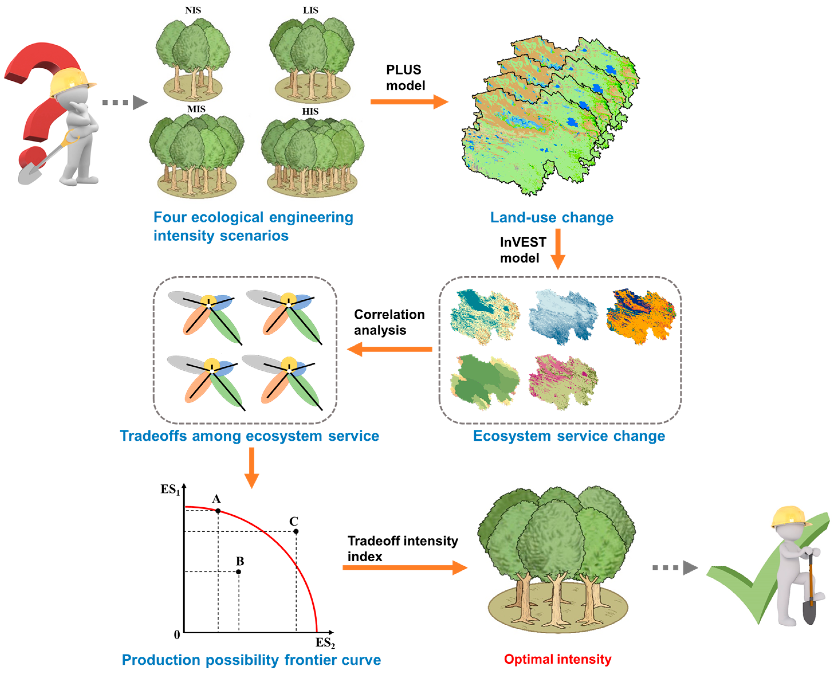
2. Materials and Methods

We first designed four land-use scenarios under different EE implementation intensities using the PLUS model. Then, we used the integrated valuation of ecosystem services and tradeoffs (InVEST) model to quantify the impact of EE implementation intensities on ESs. Next, we conducted a correlation analysis to determine whether there was a tradeoff between each pair of ESs. For those ESs that had a tradeoff relationship, the PPF curve between the ESs was drawn. Finally, we determined the optimal implementation intensity by calculating the tradeoff intensity index based on the PPF curve. The general structure of this study is illustrated in Figure 1.

2.1. Study Area

Qinghai province is located in the northeastern Tibetan Plateau and the northwestern part of China at geographic coordinates 89°35’~103°04’ E and 31°36’~39°19’ N (Figure 2). The total surface area is 69,650,000 km2 (Ministry of Civil Affairs of the People’s Republic of China). The region belongs to a typical plateau continental climate zone, with an annual average precipitation between 50 mm and 450 mm and an annual average temperature between −5.1 and 9.0 °C [37]. The terrain is mainly dominated by high mountains in the north, valleys and basins in the central and western regions, and plateaus in the south [38]. The average elevation is greater than 3000 m. Qinghai province is a key freshwater supply region in China, is also called the “Chinese water tower”, and is the source of the Yangtze, Yellow, and Lancang rivers [39]. The vegetation types in Qinghai province are abundant and diverse. The vertical and horizontal zonal distribution is particularly obvious in the Qilian mountains [40]. Among the forest resources in Qinghai province, natural forest resources account for 95.82% of the total forest area, and the area of planted forests is very small [41]. The core goal of EE in Qinghai province is to protect the forest ecosystem.

2.2. Data Collections

Our study collected multi-source data, such as land-use, meteorological, DEM (Digital Elevation Model), soil, population density, and GDP (Gross Domestic Product) data, to run the models. For land-use data in 2010 and 2020, we used ENVI 5.3 software to identify the LULC types by a maximum-likelihood algorithm based on the supervised classification. Qinghai province exhibited all 11 land classification types, namely farmland, forest, natural shrub, sparse woodland, natural grassland, water, snow, built-up land, bare land, desertification land, and wetland (Figure 1 and Table S7). Since the similar spectral characteristics of natural and planted forests in remote sensing interpretation made them difficult to distinguish, the forest type included natural forests and plantations. By verifying with ground testing samples, the overall interpretation accuracy was not less than 85%. To reduce the error caused by climate factors, we used the average climate data across 40 years to evaluate ESs. The data sources, data processing, and related detailed description of the other data required for this study are available in Tables S1 and S3. All layers were resampled to a 1 km resolution, and the projected coordinate system was unified to the WGS 1984 UTM Zone 47N for consistent analysis.

2.3. Land-Use Simulation

2.3.1. PLUS Model

We used the PLUS model to predict the land-use pattern in Qinghai province in 2030 [42]. The PLUS model integrates a rule-mining framework based on a land expansion analysis strategy (LEAS) and a cellular automata (CA) model based on multi-type random patch seeds (CARS) [43] to analyze landscape dynamics. This approach accurately simulates the intrinsic nonlinear relationships of land-use patch-level changes to improve the previous models [30]. Compared with other CA models, the simulation results of the PLUS model are more accurate, and the landscape pattern is more realistic [42].
The PLUS model extracts the expansion parts of each land-use type in the two periods and uses the random forest algorithm to obtain the suitability probability of each land-use type in LEAS, and then predicts the future landscape pattern in CARS [31]. Based on the conditions in Qinghai province and data accessibility, we calculated the suitability probability of each land-use type in the LEAS module by using 13 driving factors and land-use expansion data. The driving factors included 6 natural factors (temperature, precipitation, elevation, slope, terrain undulation, and soil type), 2 socioeconomic factors (GDP and population density), and 5 accessibility factors (the proximity to open water, roads, railways, rivers, and lakes). The CARS module operation requires two parameters, including the transition matrix and neighborhood weights. The transition matrix includes values of 0 (one land-use type cannot be transformed into another), and 1 (one land-use type can be transformed). The neighborhood weight indicates the expansion intensity of different land-use types, and its value range is 0–1. The closer the weight is to 1, the stronger the expansion intensity of the land-use type. In this study, the land-use transition matrix and the change ratios of land-use types from 2010 to 2020 were used to represent the transition matrix and the neighborhood weights of the corresponding land-use types from 2020 to 2030. We thus set the transition matrix shown in Table S4 and the neighborhood weights in Table S5.

2.3.2. PLUS Model Validation

To validate the PLUS model, we first simulated the spatial distribution of land use in 2020 based on that of 2010, and compared the simulation results with factual data from the same year. The Kappa coefficient was relatively reliable because it considered the proportion of cells that were correctly classified due to chance [44]. The figure of merit (FOM) was able to measure the performance of the model in simulating the changing part of the land use and provided a more precise indication of the model’s ability [44]. Thus, we selected the Kappa coefficient and FOM to validate the accuracy of the simulation results. The closer the Kappa coefficient was to 1, and the greater the FOM value was above 0.15, the higher the simulation accuracy was.

2.3.3. EE Implementation Intensity Scenarios

Combined with the development status, related government documents [35], and the Fourteenth Five-Year Plan of Qinghai province, we set four intensity scenarios of EE implementation in 2030 based on the historical pattern of land-use changes in 2010–2020 (Table S8). The four scenarios were as follows: (1) natural implementation scenario (NIS): the land use changed at a constant rate consistent with that of 2010–2020; (2) low-intensity implementation scenario (LIS): the forests were planted by increasing the transition probability of farmland, bare land, and desertification land shifting to forest and natural shrub by 10%, and protected by decreasing the transition probability of forest and natural shrub shifting to farmland, bare land, and desertification land by 10%; (3) medium-intensity implementation scenario (MIS): the transition probability increased by 30% in the planting of forests; and (4) high-intensity implementation scenario (HIS): the transition probability increased by 50% in the planting of forests. The transition probability setting for the MIS and HIS was consistent with the LIS for the protection of forests. Based on the ‘Qinghai Province Water Pollution Prevention and Control Work Plan’, in recent years, the government has emphasized the priority of natural protection and restoration, and highlighted the protection of glaciers, snow, and lakes. Therefore, we also limited the expansion of open water and snow and kept the built-up land unchanged. The land demand amounts under four scenarios were shown in Table S6.

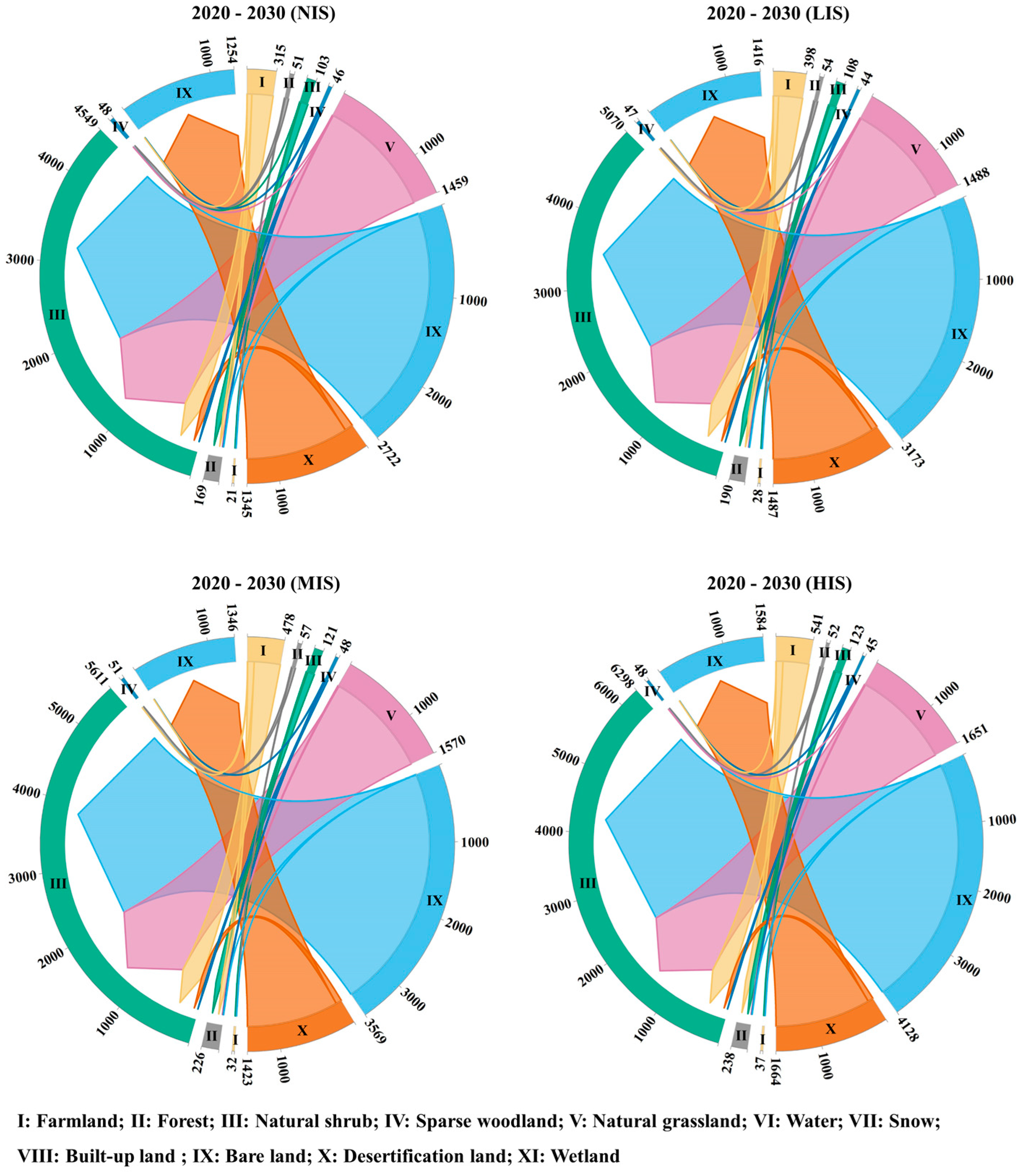
2.3.4. Land-Use Type Changes

We calculated the rate of land-use change to quantify the various land-type changes under four scenarios [45]. The calculation formula is as follows:
T i = T i t T i t 1
r i = T i t T i t 1 T i t 1
where T i is the change to areas of land of type i . T i t is the area of land for type i in year t. T i t 1 is the area of land of type i in the previous year t. r i is the area’s rate of change for land type i .

2.4. Quantifying Ecosystem Services

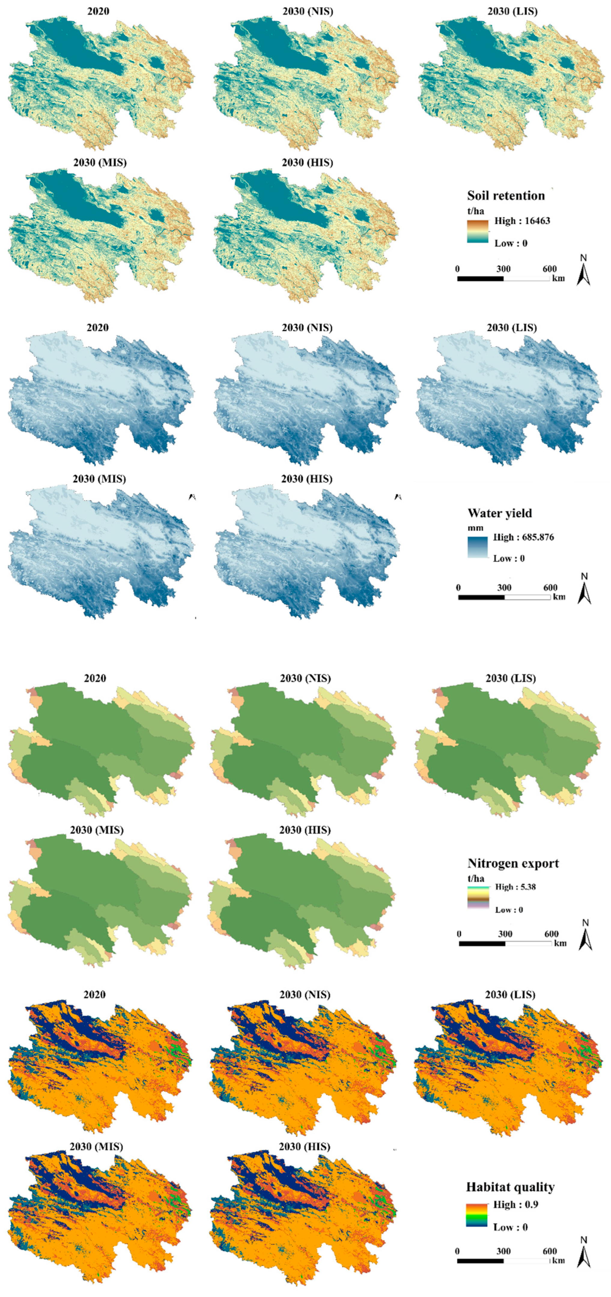
2.4.1. Ecosystem Service Selection and Evaluation

We selected ESs based on the ES classification framework [46], the Common International Classification of Ecosystem Services (CICES) [47], the questionnaire of Qinghai residents [21], and the environmental conditions in the study area. Although Qinghai province provided extensive ESs, soil erosion and water resource shortages were major environmental problems. Thus, we considered water-related ESs, including soil retention (SR), water yield (WY), and water purification (WP). Moreover, the Three-River Headwaters National Park in Qinghai province has many species and a large amount of wildlife; thus, it is necessary to evaluate the habitat quality (HQ). Of course, it is also necessary to evaluate carbon storage (CS). Therefore, we finally selected five ESs, namely SR, WY, WP, HQ, and CS (more detailed information on the ES selection can be found in Yan, Wang, Li, Wang, Jin, Jiang, Yang and Wang [21]).
The InVEST model is a comprehensive model that simulates the changes in the quality and value of ESs under different land-use scenarios, aiming to provide a scientific basis for decision makers [48]. The model has been widely used to assess natural capital and ESs, and has achieved good effects in the United States [49], China [50], and other countries [29,51]. It includes many modules for evaluation. In this study, we selected the sediment delivery ratio module (for SR), the WY module (for WY), the nutrient delivery ratio module (for WP), the habitat quality module (for HQ), and the carbon storage and sequestration module (for CS) to evaluate the ESs in 2020 and 2030 under different scenarios in Qinghai province. A detailed description of the quantitative ESs process is shown in Supplementary Information A. The relevant input parameters and settings were shown in Tables S1 and S2.

2.4.2. InVEST Model Validation

Based on the yearly hydrological monitoring data of sediment export and WY from twenty-three hydrological stations, the sediment delivery ratio module and WY module were validated. For the nutrient delivery ratio module, when setting the nitrogen load value, we referred to many parameters from the literature [52,53] and the InVEST user guide (Table S2) to reduce the module’s error. We simulated the suitable habitats of twenty-two species, including seven birds, thirteen other instances of wildlife, and two endangered plants, using the maximum entropy model to validate the HQ module. Since we used the observed data in the process of assessing carbon storage, it did not need to be verified.

2.4.3. Ecosystem Services Tradeoff Analysis

Correlation analysis (Pearson’s r ) was used to estimate the relationships among ESs under different EE implementation scenarios. Based on the specific resolution requirements, we randomly generated 65,000 points in the study area to obtain sufficient data samples. A negative correlation between ESs ( p < 0.05) was considered a tradeoff relationship, while a positive correlation was regarded as a synergistic relationship.

2.5. Determining an Optimal EE Implementation Intensity

2.5.1. Production Possibility Frontier Curve

The PPF curve can quantitatively describe the degree of tradeoff between the two outputs [33]. If ES combination points are below the curve, it indicates that resource utilization is insufficient and land use has optimization potential. If ES combination points are on the curve, land use is in an optimal configuration. If the points are above the curve, then ESs exceed the optimal allocation, but this situation is difficult to achieve with existing resources and technical conditions.
We first estimated the five ESs in Qinghai province and normalized the ESs to a range of 0–1. Second, the five normalized layers were superimposed to obtain the total ES value for each grid. We arranged the total ES values in ascending order, and selected the grids with larger ES values. Two tradeoff ESs values corresponding to these selected grids were extracted to fit the PPF curve.

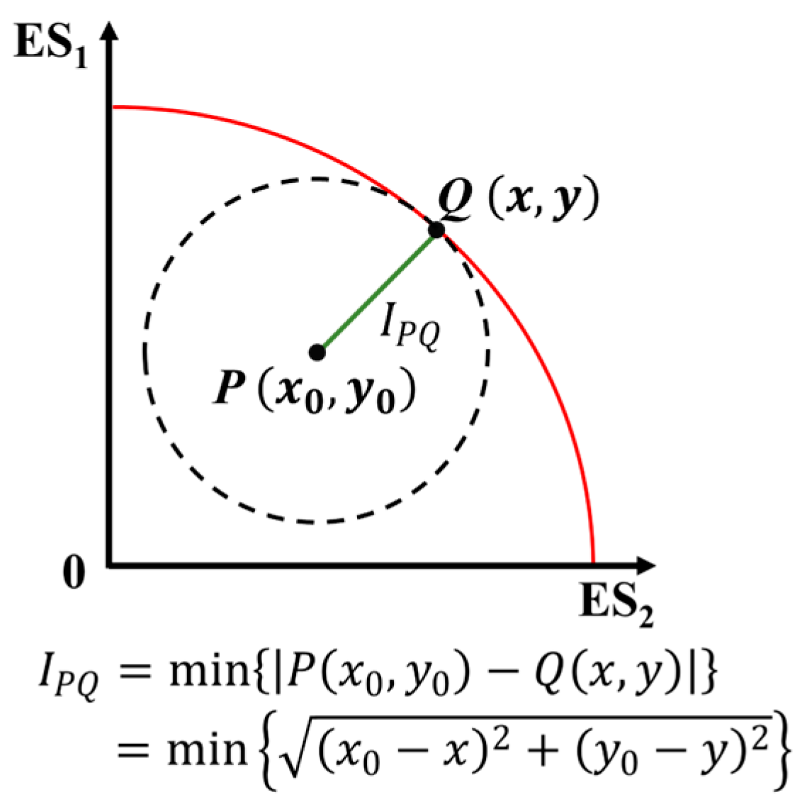
2.5.2. Tradeoff Intensity Index

If the tradeoff direction is selected to optimize the combination of the two services, the optimal state can be viewed as an equilibrium state. Only one optimal state can be attained within a specified set of conditions; that is, only one PPF curve can be obtained [54]. If P represents the point corresponding to the mean value of two tradeoff ESs, its coordinate is x 0 , y 0 . We assume that the expression of the PPF curve is y = f x , and use point P x 0 , y 0 as the center and I P Q as the radius to make a circle. The circle has only one intersection point Q x , y ) with the PPF curve. The shortest distance ( I P Q ) from the mean value of the two tradeoff ESs ( P x 0 , y 0 ) to the PPF curve ( Q x , y ) ) represents the tradeoff intensity index (Figure 3) [33].

3. Results

3.1. Spatiotemporal Changes in Future Land Use

Under all land-use scenarios, forest, natural shrub, and sparse woodland significantly increased (Figure 4), while farmland, bare land, and desertification land significantly decreased from 2020 to 2030. Under the NIS, LIS, MIS, and HIS scenarios, natural shrubs increased the most; from 2020 to 2030, they increased by 13.34%, 14.22%, 15.57%, and 16.93%, respectively (Figure 5). Natural shrubs were mainly transferred from natural grassland, bare land, and farmland and were mainly distributed in the central and western regions. The forest area increased from 2020 to 2030 with rates of 6.71%, 7.09%, 7.42%, and 7.79%, respectively, for the four scenarios. Forest was mainly converted from natural shrub, farmland, sparse woodland, and bare land and was mainly located in the central and eastern regions. Compared with 2020, the area of desertification land consistently decreased, with rates of 6.89%, 6.93%, 6.98%, and 7.04%, respectively. The area of bare land also decreased by 1.54%, 1.82%, 2.24%, and 2.67%, respectively.

3.2. Model Validation

For the PLUS model, the calculated Kappa coefficient between simulated and observed land use in 2020 was 0.844, and the FOM was 0.385, indicating that the PLUS model had high reliability. For the InVEST model, strong linear relationships were exhibited between the observed data and the predicted data for the sediment export and WY, with R2 values of 0.790 and 0.932 (p < 0.001) (Figure 6). For HQ, the results revealed that 60.10% of the appropriate habitats replicated by the two models were congruous.

3.3. Ecosystem Service Changes under Different Scenarios

A high provision of SR was found in the eastern and southern regions. This was mainly because of the flat slope and larger areas of forest, natural grassland, and natural shrub (Figure 7). Northwestern regions were mainly dominated by bare land, causing serious soil loss, and thus had a low amount of SR. Under the NIS, LIS, MIS, and HIS scenarios, the SR increased from 2020 to 2030 by 0.05%, 0.06%, 0.07%, and 0.08%, respectively. SR changes were directly related to the natural shrub and forest areas (Figure S1). As the EE implementation intensity increased, vegetation coverage increased, leading to a significant increase in SR.
The distribution trend in WY was consistent with that of precipitation. The WY with high provision was mainly located in the southern and northeastern regions. Areas with lower value were mainly located in the northwestern and central regions. The WY decreased by 2.59%, 2.91%, 3.15%, and 3.46%, respectively, for the four scenarios. Due to the increase in vegetation coverage, evapotranspiration significantly increased in the eastern region, and, thus, the WY decreased.
We used the nitrogen export to represent the capacity of WP. The higher the nitrogen export value, the worse the WP capacity was. Due to the lower nitrogen export in the central region, the WP in the central regions was higher than that of the other regions. This was mainly because farmland and built-up land were located in the eastern region, resulting in an increase in nitrogen export. For the NIS, LIS, MIS, and HIS, the nitrogen export decreased by 1.13%, 1.19%, 1.24%, and 1.35%, respectively. Due to the enhancement of WP capacity caused by the increase in the vegetation coverage and the reduction of the pollutant load caused by the decrease in farmland, WP significantly improved.
HQ was higher in the eastern, southern, and central regions because these regions had a higher natural shrub coverage and a lower degree of habitat fragmentation. The lower HQ areas were distributed in the regions with bare land, which has a fragile ecological environment. The mean HQ index was 0.568 in 2020, and predicted to be 0.574, 0.575, 0.576, and 0.577 under the NIS, LIS, MIS, and HIS in 2030, respectively. As the natural shrub and forest areas increased, better habitat conditions were provided for animals and plants, and thus the HQ index also increased.
The distribution trend of CS was higher in the eastern region than in the northwestern region because of the higher vegetation coverage. Compared to 2020, CS increased under the NIS, LIS, MIS, and HIS in 2030 by 1.32%, 1.40%, 1.53%, and 1.65%, respectively.

3.4. Tradeoffs among Ecosystem Services

There were some significant tradeoffs and synergies among the five ESs across the different scenarios (Table S9). Compared to 2020, when SR showed an increasing trend due to the expansion of forests and shrubs in all scenarios for 2030, HQ and CS also showed an increasing trend, while the WY and nitrogen export showed the opposite. Due to the inverse relationship between nitrogen export and WP, the relationships between WP and the other ESs were opposite to the relationships between nitrogen export and the other ESs. Therefore, WY showed a significantly negative correlation with SR, HQ, CS, and WP (p < 0.01) under all scenarios, indicating WY had tradeoff relationships with the other four ESs. There were significant positive correlations between SR, CS, WP, and HQ (p < 0.01).

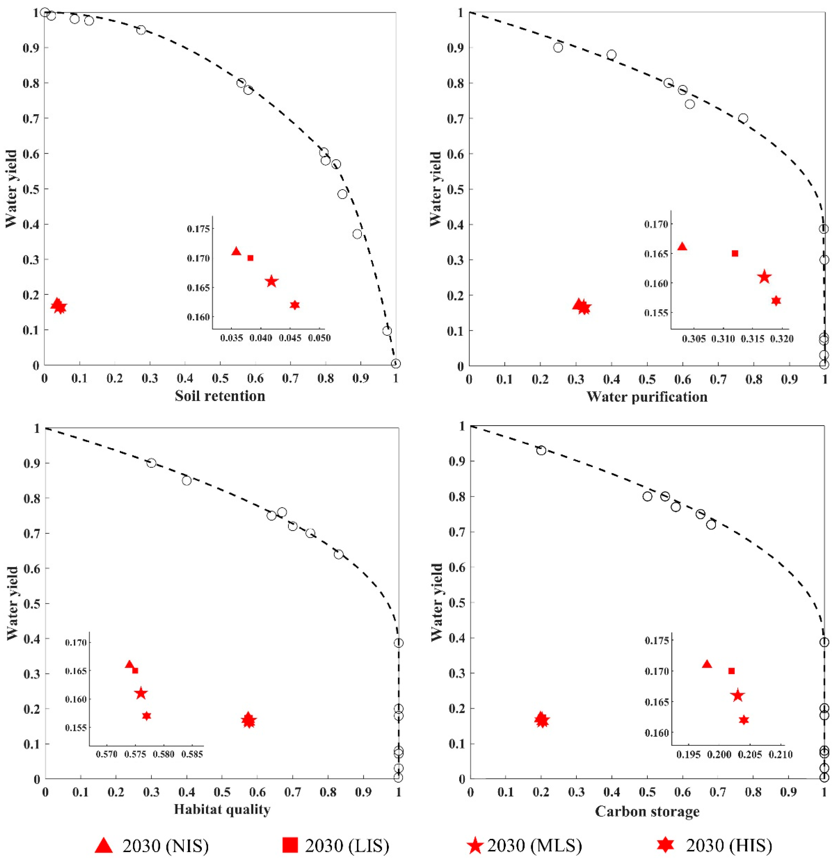
3.5. PPF Curves among Ecosystem Service Tradeoffs

To determine the optimal EE implementation intensity, we fitted the PPF curves of the two ESs in the different scenarios based on their tradeoff relationships (Figure 8). The simulated value corresponding to the grid with the larger value was consistent under all scenarios, and, thus, the PPF curves coincided completely. Four PPF curves presented a downward-convex curve between two tradeoff ESs. The PPF curve between WY and SR was divided into two phases: a small tradeoff phase where the curve changed slowly for the SR in the range of 0–0.8 and a large tradeoff phase where the curve changed rapidly for the SR in the range of 0.8–1. Similar relationships were also observed between WY and WP, HQ, and CS. When the WY was in the range of 0.4–1, the curves for WP, HQ, and CS showed a slow downward trend. When the WY was in the range of 0–0.4, the values of the other three ESs were at their maximum, and the curve showed a vertical line, indicating the tradeoffs increased significantly.
The tradeoff intensity index among the two ESs was different in different scenarios (Table 1). Only for WY versus HQ did the HIS have the lowest tradeoff intensity index (0.4235). Between WY and SR, WP, and CS, the LIS had the lowest tradeoff intensity index, with values of 0.8138, 0.6695, and 0.7175, respectively. This result indicated that under the LIS, the ES combination points were nearest to the PPF curve, showing an optimal effect of the tradeoff relationship among ESs. Therefore, the LIS was the optimal scenario of EE implementation in Qinghai province.

4. Discussion

4.1. Impact of EE Implementation Intensities on ESs

Land-use change is the most important factor influencing ES changes [7], and EE is the dominant element in the land-use change of Qinghai province [21]. In this study, we simulated land-use changes from 2020 to 2030 under four EE implementation intensities and evaluated their impacts on ESs in Qinghai province, China. We found that land-use changes under different scenarios had obvious similarities, but there were also some differences. EE implementation promoted conversions from farmland, bare land, and desertification land to natural shrubs and forests. The higher the EE implementation intensity, the greater the conversion rate. The expansion of natural shrubs and forests was also predicted in the central region of Qinghai province under the four scenarios. Suitable climate conditions with more precipitation and flatter terrain would promote an increase in vegetation coverage.
The results of our simulations revealed that the increase in vegetation coverage with EE implementation intensity contributed to maintaining SR, increasing CS, and improving HQ. However, it was not conducive to forming runoff, and, thus, it reduced the WY. Farmland was the major contributor to the nitrogen export, and a decline in farmland would reduce the nitrogen export and thus increase the WP. Many regions have also implemented EE in the past 20 years, such as the forest region of northeastern China [55] and southwestern China [22], indicating that EE can promote the renewed growth of vegetation and enhance ecological function. In general, EE is an effective way to improve the ESs and human well-being.
Although EE has provided significant ecological benefits, decision-makers also need to carefully consider the negative impacts caused by EE implementation, such as a reduction in WY [21]. Climate change is the main reason for WY changes [49,56]. However, in regions with less precipitation, such as Qinghai province, the impact of expanding vegetation cover on WY is a serious concern. The results of our simulations showed that the five ESs had complex tradeoff relationships under different EE implementation intensities. The tradeoffs between WY and the other ESs (i.e., SR, HQ, CS, and WP) were more obvious with higher EE implementation intensities. Our findings are consistent with previous studies [21,27,57]. Due to the complex tradeoff relationship among ESs, it is almost impossible for various ESs to increase or decrease simultaneously in the implementation of EE. Policy-makers cannot strengthen some ESs and ignore other ESs, especially those that human beings can benefit directly from. To ensure the long-term sustainability of EE, the relationship between economic development and ecological protection must be balanced. By setting up scenarios with different implementation intensities and conducting simulations, land-use changes at various intensities and their impacts on ESs can be predicted. This scientific prediction and quantitative assessment method helps find an optimal balance between ecological protection and economic development. Therefore, the balance between various ESs must be comprehensively considered in EE planning and decision-making to better guide ecological construction.

4.2. Determining the Optimal EE Implementation Scenario Based on PPF

The win-win situation of multifunctional ecosystems via the implementation of the appropriate EE intensity is a necessary condition for sustainable development [17]. Previous studies only explored the impact of land-use change driven by EE on various ESs through scenario simulation to find a suitable land-use pattern [27,58]. This method had a certain degree of subjectivity. Our study calculated the tradeoff intensity index to select an optimal EE intensity by combining the scenario simulation with PPF curves, which can provide quantitative guidance for the selection of the optimal implementation intensity. This comprehensive approach helps policy-makers better understand the impact of different policy decisions on ecosystems and land use, thereby formulating more scientific and sustainable development strategies.
The four fitted PPF curves show that the implementation of different intensities of EE leads to various ESs having different change rates and even changing directions in Qinghai province. The MIS and the HIS had a higher tradeoff intensity index, indicating that the tradeoffs between the provisioning services and the regulating services were significant, consistent with the findings of Ma et al. [58]. However, under the LIS, even though the function of the ES was not fully developed, the appropriate intensity increases promoted a relatively good balance among the ESs. Thus, we chose the LIS with a lower tradeoff intensity index as the optimal scenario for the balanced development of multiple ecosystem functions. It is worth noting that ecosystems are dynamic and may exhibit different service demands and tradeoffs at different temporal and spatial scales. By regularly evaluating and adjusting the PPF curve, we can promptly respond to changes in social needs, and improve the flexibility and adaptability of ecological management.

4.3. Limitations and Future Research

The current study developed a framework for determining the optimal EE implementation intensity to help policy-makers enact appropriate land management. However, some uncertainties and limitations remain. First, different ESs, including supplying, supporting, cultural, and regulating services, have different tradeoff relationships. Our study mainly evaluated the impacts of EE implementation on five ESs and explored the relationship between sets of two ESs. Thus, integrating diverse ESs into a framework and considering interactions among ESs in practical EE applications to guide land management should be further researched and explored. Secondly, the PPF should contain as many production-possibility data points as possible. We only simulated land-use changes under four EE implementation intensities based on the development planning of Qinghai province in 2030. Dozens or even hundreds of scenarios should be designed to analyze the ES tradeoffs to obtain the optimal scenario. Therefore, it is necessary to gradually establish a set of frameworks combined with more scenario analyses based on regional practical situations to fit a perfect PPF curve to provide critical knowledge for achieving optimal land-use allocation. Third, due to the complexity and uncertainties of EE investment, our methods did not consider the cost of increasing the vegetation cover by tree or shrub plantation in plateau and arid regions. This limitation should be considered in future studies.

5. Conclusions

In this study, we applied a methodology using the PLUS model, the InVEST model, and the PPF curve to model the land-use changes and analyze the ES tradeoffs under four EE implementation intensities in Qinghai province from 2020 to 2030. We found that with the increase in EE implementation intensity, WY had significant tradeoff relationships with SR, HQ, CS, and WP. Based on the tradeoff intensity index, under all EE implementation scenarios, the low-intensity implementation scenario could be the optimal EE implementation intensity (406.68 km2 expansions of forest and shrub) to achieve a balance between regional economic development and the sustainable provision of ESs. We suggest that the local government should comprehensively consider the changes in ESs and their tradeoffs according to regional ecological goals and geographical factors when formulating EE policies to realize a sustainable supply of ESs. Our study proposed a novel framework to effectively determine the investment in EE and the return in ESs for policymakers.

Supplementary Materials

The following supporting information can be downloaded at https://www.mdpi.com/article/10.3390/land13060848/s1: Table S1: Data requirements for the InVEST models; Table S2: Key parameters used in biophysical table of modules; Table S3: Data requirements for the PLUS models; Table S4: Transition matrix for CARS module operation in the PLUS model; Table S5: Neighborhood weights for CARS module operation in the PLUS model; Table S6: Land demand amounts under four scenarios; Table S7: LULC classes used in the maps for Qinghai province; Table S8: Land-use composition in Qinghai province in 2010 and 2020; Table S9: Pearson correlation among five ESs under different implementation intensity scenarios; Figure S1: Spatial changes of the five ESs under different scenarios from 2020 to 2030; Supplement S1: InVEST model processes; Supplement S2: Data requirements; Supplement S3: LULC classes and composition; Supplement S4: Ecosystem services changes; Supplement S5: Ecosystem services tradeoffs. References [48,59,60,61,62,63,64,65,66,67,68,69] are cited in the supplementary materials.

Author Contributions

Conceptualization, K.Y. and W.W.; methodology, K.Y., B.Z. and J.J. (Jiaxin Jin); software, K.Y., B.Z. and R.W.; validation, J.J. (Jiaxin Jin), J.J. (Jiang Jiang), W.D. and T.W.; formal analysis, K.Y.; investigation, K.Y.; resources, W.W.; data curation, K.Y., X.W., J.J. (Jiaxin Jin) and T.W.; writing—original draft preparation, K.Y.; writing—review and editing, X.W., J.J. (Jiaxin Jin), J.J. (Jiang Jiang), W.D., R.W., H.Y., T.W. and W.W.; visualization, K.Y.; supervision, Y.L. and W.W.; project administration, Y.L. and W.W.; funding acquisition, W.W. All authors have read and agreed to the published version of the manuscript.

Funding

This research was funded by the National Key Research and Development Program of China (No. 2021YFD2200404), the Research and Innovation Project of Northwest Surveying and Planning Institute of National Forestry and Grassland Administration (No. XBJ-KJCX-2021-16), the China Scholarship Council (No. 202208320373), the Postgraduate Research and Practice Innovation Program of Jiangsu Province (No. KYCX21_0869), and the Priority Academic Program Development of Jiangsu Higher Education Institutions (PAPD).

Data Availability Statement

The original contributions presented in this study are included in the article; further inquiries can be directed to the corresponding author.

Acknowledgments

Special thanks to Shuiqiang Yu, Yanrong Yang, Leying Zhang, and Cheng Hu for their useful discussions and comments. We thank the anonymous reviewers and academic editor for the invaluable suggestions.

Conflicts of Interest

The authors declare no conflicts of interest.

References

  1. Costanza, R.; d’Arge, R.; de Groot, R.; Farber, S.; Grasso, M.; Hannon, B.; Limburg, K.; Naeem, S.; O’Neill, R.V.; Paruelo, J.; et al. The value of the world’s ecosystem services and natural capital. Nature 1997, 387, 253–260. [Google Scholar] [CrossRef]
  2. Daily, G.C.; Söderqvist, T.; Aniyar, S.; Arrow, K.; Dasgupta, P.; Ehrlich, P.R.; Folke, C.; Jansson, A.; Jansson, B.-O.; Kautsky, N.; et al. The value of nature and the nature of value. Science 2000, 289, 395–396. [Google Scholar] [CrossRef]
  3. Niu, L.; Shao, Q.; Ning, J.; Huang, H. Ecological changes and the tradeoff and synergy of ecosystem services in western China. J. Geogr. Sci. 2022, 32, 1059–1075. [Google Scholar] [CrossRef]
  4. Ouyang, Z.; Song, C.; Zheng, H.; Polasky, S.; Xiao, Y.; Bateman, I.J.; Liu, J.; Ruckelshaus, M.; Shi, F.; Xiao, Y.; et al. Using gross ecosystem product (GEP) to value nature in decision making. Proc. Natl. Acad. Sci. USA 2020, 117, 14593–14601. [Google Scholar] [CrossRef]
  5. Díaz-Yáñez, O.; Pukkala, T.; Packalen, P.; Lexer, M.J.; Peltola, H. Multi-objective forestry increases the production of ecosystem services. For. Int. J. For. Res. 2021, 94, 386–394. [Google Scholar] [CrossRef]
  6. Xie, G.; Zhen, L.; Lu, C.-X.; Xiao, Y.; Chen, C. Expert knowledge based valuation method of ecosystem services in China. J. Nat. Resour. 2008, 23, 911–919. [Google Scholar]
  7. Zheng, H.; Peng, J.; Qiu, S.; Xu, Z.; Zhou, F.; Xia, P.; Adalibieke, W. Distinguishing the impacts of land use change in intensity and type on ecosystem services trade-offs. J. Environ. Manag. 2022, 316, 115206. [Google Scholar] [CrossRef]
  8. Evans, N.M.; Carrozzino-Lyon, A.L.; Galbraith, B.; Noordyk, J.; Peroff, D.M.; Stoll, J.; Thompson, A.; Winden, M.W.; Davis, M.A. Integrated ecosystem service assessment for landscape conservation design in the Green Bay watershed, Wisconsin. Ecosyst. Serv. 2019, 39, 101001. [Google Scholar] [CrossRef]
  9. Bryan, B.A.; Gao, L.; Ye, Y.Q.; Sun, X.F.; Connor, J.D.; Crossman, N.D.; Stafford-Smith, M.; Wu, J.G.; He, C.Y.; Yu, D.Y.; et al. China’s response to a national land-system sustainability emergency. Nature 2018, 559, 193–204. [Google Scholar] [CrossRef]
  10. Sannigrahi, S.; Chakraborti, S.; Joshi, P.K.; Keesstra, S.; Sen, S.; Paul, S.K.; Kreuter, U.; Sutton, P.C.; Jha, S.; Dang, K.B. Ecosystem service value assessment of a natural reserve region for strengthening protection and conservation. J. Environ. Manag. 2019, 244, 208–227. [Google Scholar] [CrossRef]
  11. Liu, G.; Zhang, F. Land Zoning Management to Achieve Carbon Neutrality: A Case Study of the Beijing–Tianjin–Hebei Urban Agglomeration, China. Land 2022, 11, 551. [Google Scholar] [CrossRef]
  12. Paillex, A.; Schuwirth, N.; Lorenz, A.W.; Januschke, K.; Peter, A.; Reichert, P. Integrating and extending ecological river assessment: Concept and test with two restoration projects. Ecol. Ind. 2017, 72, 131–141. [Google Scholar] [CrossRef]
  13. Vogler, K.C.; Ager, A.A.; Day, M.A.; Jennings, M.; Bailey, J.D. Prioritization of Forest Restoration Projects: Tradeoffs between Wildfire Protection, Ecological Restoration and Economic Objectives. Forests 2015, 6, 4403–4420. [Google Scholar] [CrossRef]
  14. Puspitaloka, D.; Kim, Y.-S.; Purnomo, H.; Fule, P.Z. Defining ecological restoration of peatlands in Central Kalimantan, Indonesia. Restor. Ecol. 2020, 28, 435–446. [Google Scholar] [CrossRef]
  15. Fu, H.; Yan, Y. Ecosystem service value assessment in downtown for implementing the “Mountain-River-Forest-Cropland-Lake-Grassland system project”. Ecol. Ind. 2023, 154, 110751. [Google Scholar] [CrossRef]
  16. Lu, F.; Hu, H.F.; Sun, W.J.; Zhu, J.J.; Liu, G.B.; Zhou, W.M.; Zhang, Q.F.; Shi, P.L.; Liu, X.P.; Wu, X.; et al. Effects of national ecological restoration projects on carbon sequestration in China from 2001 to 2010. Proc. Natl. Acad. Sci. USA 2018, 115, 4039–4044. [Google Scholar] [CrossRef]
  17. Xu, C.; Jiang, Y.; Su, Z.; Liu, Y.; Lyu, J. Assessing the impacts of Grain-for-Green Programme on ecosystem services in Jinghe River basin, China. Ecol. Ind. 2022, 137, 108757. [Google Scholar] [CrossRef]
  18. Wei, C.; Dong, X.; Yu, D.; Liu, J.; Reta, G.; Zhao, W.; Kuriqi, A.; Su, B. An alternative to the Grain for Green Program for soil and water conservation in the upper Huaihe River basin, China. J. Hydrol. Reg. Stud. 2022, 43, 101180. [Google Scholar] [CrossRef]
  19. Wang, X.F.; Zhang, X.R.; Feng, X.M.; Liu, S.R.; Yin, L.C.; Chen, Y.Z. Trade-offs and synergies of ecosystem services in karst area of China driven by Grain-for-Green program. Chin. Geogr. Sci. 2020, 30, 101–114. [Google Scholar] [CrossRef]
  20. Qiao, D.; Yuan, W.T.; Ke, S.F. China’s Natural Forest Protection Program: Evolution, impact and challenges. Int. For. Rev. 2021, 23, 338–350. [Google Scholar] [CrossRef]
  21. Yan, K.; Wang, W.; Li, Y.; Wang, X.; Jin, J.; Jiang, J.; Yang, H.; Wang, L. Identifying priority conservation areas based on ecosystem services change driven by Natural Forest Protection Project in Qinghai province, China. J. Clean. Prod. 2022, 362, 132453. [Google Scholar] [CrossRef]
  22. Wu, S.; Li, J.; Zhou, W.; Lewis, B.J.; Yu, D.; Zhou, L.; Jiang, L.; Dai, L. A statistical analysis of spatiotemporal variations and determinant factors of forest carbon storage under China’s Natural Forest Protection Program. J. For. Res. 2018, 29, 415–424. [Google Scholar] [CrossRef]
  23. Fu, Q.; Li, B.; Hou, Y.; Bi, X.; Zhang, X.S. Effects of land use and climate change on ecosystem services in Central Asia’s arid regions: A case study in Altay Prefecture, China. Sci. Total Environ. 2017, 607, 633–646. [Google Scholar] [CrossRef]
  24. Zheng, D.F.; Wang, Y.H.; Hao, S.; Xu, W.J.; Lv, L.T.; Yu, S. Spatial -temporal variation and tradeoffs/synergies analysis on multiple ecosystem services: A case study in the Three -River Headwaters region of China. Ecol. Ind. 2020, 116, 106494. [Google Scholar] [CrossRef]
  25. Wang, Y.; Zhou, L.H.; Yang, G.J.; Guo, R.; Xia, C.Z.; Liu, Y. Performance and obstacle tracking to Natural Forest Resource Protection Project: A rangers’ case of Qilian mountain, China. Int. J. Environ. Res. Public Health 2020, 17, 5672. [Google Scholar] [CrossRef]
  26. Li, C.; Wu, Y.; Gao, B.; Zheng, K.; Wu, Y.; Li, C. Multi-scenario simulation of ecosystem service value for optimization of land use in the Sichuan-Yunnan ecological barrier, China. Ecol. Ind. 2021, 132, 108328. [Google Scholar] [CrossRef]
  27. Peng, J.; Hu, X.X.; Wang, X.Y.; Meersmans, J.; Liu, Y.X.; Qiu, S.J. Simulating the impact of Grain-for-Green Programme on ecosystem services trade-offs in Northwestern Yunnan, China. Ecosyst. Serv. 2019, 39, 100998. [Google Scholar] [CrossRef]
  28. Bai, Y.; Wong, C.P.; Jiang, B.; Hughes, A.C.; Wang, M.; Wang, Q. Developing China’s ecological redline policy using ecosystem services assessments for land use planning. Nat. Commun. 2018, 9, 3034. [Google Scholar] [CrossRef]
  29. Hoque, M.Z.; Cui, S.; Islam, I.; Xu, L.; Ding, S. Dynamics of plantation forest development and ecosystem carbon storage change in coastal Bangladesh. Ecol. Ind. 2021, 130, 107954. [Google Scholar] [CrossRef]
  30. Zhang, S.; Zhong, Q.; Cheng, D.; Xu, C.; Chang, Y.; Lin, Y.; Li, B. Landscape ecological risk projection based on the PLUS model under the localized shared socioeconomic pathways in the Fujian Delta region. Ecol. Ind. 2022, 136, 108642. [Google Scholar] [CrossRef]
  31. Zhai, H.; Lv, C.; Liu, W.; Yang, C.; Fan, D.; Wang, Z.; Guan, Q. Understanding spatio-temporal patterns of land use/land cover change under urbanization in Wuhan, China, 2000–2019. Remote Sens. 2021, 13, 3331. [Google Scholar] [CrossRef]
  32. Guo, M.; Ma, S.; Wang, L.J.; Lin, C. Impacts of future climate change and different management scenarios on water-related ecosystem services: A case study in the Jianghuai ecological economic Zone, China. Ecol. Ind. 2021, 127, 107732. [Google Scholar] [CrossRef]
  33. Yang, W.; Jin, Y.; Sun, T.; Yang, Z.; Cai, Y.; Yi, Y. Trade-offs among ecosystem services in coastal wetlands under the effects of reclamation activities. Ecol. Ind. 2018, 92, 354–366. [Google Scholar] [CrossRef]
  34. Aryal, K.; Maraseni, T.; Apan, A. How much do we know about trade-offs in ecosystem services? A systematic review of empirical research observations. Sci. Total Environ. 2022, 806, 151229. [Google Scholar] [CrossRef]
  35. Yang, X.; Li, Y.; Wang, R.; Wang, X.; Li, H.; Dong, W.; Lei, Y.; Xin, J.; Yang, Z.; Wang, J. Construction and Application of Natural Forest Resources Protection Project Evaluation System in Qinghai Province; National Scientific and Technological Achievements, Qinghai Province Natural Forest Protection Center: Qinghai, China, 2022. [Google Scholar]
  36. Jiang, C.; Li, D.Q.; Wang, D.W.; Zhang, L.B. Quantification and assessment of changes in ecosystem service in the Three-River Headwaters Region, China as a result of climate variability and land cover change. Ecol. Ind. 2016, 66, 199–211. [Google Scholar] [CrossRef]
  37. Wang, X.; Wang, K.; Lin, F.; Guo, K. Preliminary report on the landslide early warning on 20 August 2021, in Nangqian County, Qinghai Province, China. Sci. Rep. 2022, 12, 9795. [Google Scholar] [CrossRef] [PubMed]
  38. Lin, S.; He, K.; Wang, Z.; Zuo, Y.; Cheng, C.; Zhang, J. Multifactor relationships between the forest structure and water conservation function of Picea crassifolia Kom. plantations in Qinghai Province, China. Land Degrad. Dev. 2022, 33, 2596–2605. [Google Scholar] [CrossRef]
  39. Wang, J.; Zhou, W.; Guan, Y. Optimization of management by analyzing ecosystem service value variations in different watersheds in the Three-River Headwaters Basin. J. Environ. Manag. 2022, 321, 115956. [Google Scholar] [CrossRef]
  40. Fan, Y.; Fang, C. Evolution process and obstacle factors of ecological security in western China, a case study of Qinghai province. Ecol. Ind. 2020, 117, 106659. [Google Scholar] [CrossRef]
  41. Northwest Surveying and Planning Institute of National Forestry and Grassland Administration. Evaluation of Natural Forest Resource Protection Project in Qinghai Province; Northwest Surveying and Planning Institute of National Forestry and Grassland Administration: Xi’an, China, 2021. [Google Scholar]
  42. Liang, X.; Guan, Q.; Clarke, K.C.; Liu, S.; Wang, B.; Yao, Y. Understanding the drivers of sustainable land expansion using a patch-generating land use simulation (PLUS) model: A case study in Wuhan, China. Comput. Environ. Urban. 2021, 85, 101569. [Google Scholar] [CrossRef]
  43. Jiang, Y.; Huang, M.; Chen, X.; Wang, Z.; Xiao, L.; Xu, K.; Zhang, S.; Wang, M.; Xu, Z.; Shi, Z. Identification and risk prediction of potentially contaminated sites in the Yangtze River Delta. Sci. Total Environ. 2022, 815, 151982. [Google Scholar] [CrossRef]
  44. Wang, Z.; Zeng, J.; Chen, W.X. Impact of urban expansion on carbon storage under multi-scenario simulations in Wuhan, China. Environ. Sci. Pollut. Res. 2022, 29, 45507–45526. [Google Scholar] [CrossRef] [PubMed]
  45. Liu, G.; Zhang, F. How do trade-offs between urban expansion and ecological construction influence CO2 emissions? New evidence from China. Ecol. Ind. 2022, 141, 109070. [Google Scholar] [CrossRef]
  46. Millennium. Millennium Ecosystem Assessment Synthesis Report; Island Press: Washington, DC, USA, 2005. [Google Scholar]
  47. Haines-Young, R.; Potschin-Young, M. Revision of the Common International Classification for Ecosystem Services (CICES V5.1): A policy brief. One Ecosyst. 2018, 3, e27108. [Google Scholar] [CrossRef]
  48. Sharp, R.; Tallis, H.T.; Ricketts, T.; Guerry, A.D.; Wood, S.A.; Chaplin-Kramer, R.; Nelson, E.; Ennaanay, D.; Wolny, S.; Olwero, N.; et al. InVEST 3.2.0 User’s Guide; The Natural Capital Project; Stanford University, University of Minnesota, The Nature Conservancy, and World Wildlife Fund: Stanford, CA, USA, 2015. [Google Scholar]
  49. Bai, Y.; Ochuodho, T.O.; Yang, J. Impact of land use and climate change on water-related ecosystem services in Kentucky, USA. Ecol. Ind. 2019, 102, 51–64. [Google Scholar] [CrossRef]
  50. Wang, X.; Wu, J.; Liu, Y.; Hai, X.; Shanguan, Z.; Deng, L. Driving factors of ecosystem services and their spatiotemporal change assessment based on land use types in the Loess Plateau. J. Environ. Manag. 2022, 311, 114835. [Google Scholar] [CrossRef] [PubMed]
  51. Yohannes, H.; Soromessa, T.; Argaw, M.; Dewan, A. Impact of landscape pattern changes on hydrological ecosystem services in the Beressa watershed of the Blue Nile Basin in Ethiopia. Sci. Total Environ. 2021, 793, 148559. [Google Scholar] [CrossRef] [PubMed]
  52. Deng, D.; Deng, L. Spatial distribution characteristics and control countermeasures of nitrogen load into Qinghai lake watershed. Environ. Impact Assess. 2023, 45, 84–93. [Google Scholar]
  53. Hao, C.; Chao, S.; Deng, Y.; Wen, Q.; Xin, Y.; Yang, X.; Zhang, P. Temporal and spatial distribution characteristics and source analysis of nitrogen in the yellow river basin in Qinghai province. Res. Environ. Sci. 2023, 36, 325–333. [Google Scholar]
  54. Ager, A.A.; Day, M.A.; Vogler, K. Production possibility frontiers and socioecological tradeoffs for restoration of fire adapted forests. J. Environ. Manag. 2016, 176, 157–168. [Google Scholar] [CrossRef]
  55. Wei, Y.W.; Yu, D.P.; Lewis, B.J.; Zhou, L.; Zhou, W.M.; Fang, X.M.; Zhao, W.; Wu, S.N.; Dai, L.M. Forest carbon storage and tree carbon pool dynamics under natural forest protection program in northeastern China. Chin. Geogr. Sci. 2014, 24, 397–405. [Google Scholar] [CrossRef]
  56. Li, S.; Liu, Y.; Yang, H.; Yu, X.; Zhang, Y.; Wang, C. Integrating ecosystem services modeling into effectiveness assessment of national protected areas in a typical arid region in China. J. Environ. Manag. 2021, 297, 113408. [Google Scholar] [CrossRef]
  57. Wang, J.; Peng, J.; Zhao, M.; Liu, Y.; Chen, Y. Significant trade-off for the impact of Grain-for-Green Programme on ecosystem services in North-western Yunnan, China. Sci. Total Environ. 2017, 574, 57–64. [Google Scholar] [CrossRef]
  58. Ma, S.; Qiao, Y.P.; Jiang, J.; Wang, L.J.; Zhang, J.C. Incorporating the implementation intensity of returning farmland to lakes into policymaking and ecosystem management: A case study of the Jianghuai Ecological Economic Zone, China. J. Cleaner Prod. 2021, 306, 127284. [Google Scholar] [CrossRef]
  59. Hu, L.; Ting, W.C.; Wang, G.X.; Wei, L.; Ade, L.J. Carbon sequestration of forest ecosystem vegetation in Qinghai province. Southwest China J. Agric. Sci. 2015, 28, 826–832. [Google Scholar] [CrossRef]
  60. Lu, H.; Kang, L.; Wu, J.H. Change of carbon storage in forest vegetation and current situation analysis of Qinghai pronvince in recent 20 years. Resour. Environ. Yangtze Basin 2013, 22, 1333–1338. [Google Scholar]
  61. Pan, J.H.; Zhen, L. Analysis on trade-offs and synergies of ecosystem services in arid inland river basin. Trans. Chin. Soc. Agric. Eng. 2017, 33, 280–289. [Google Scholar] [CrossRef]
  62. Pan, T.; Wu, S.H.; Dai, E.F.; Liu, Y.J. Spatiotemporal variation of water source supply service in Three Rivers Source Area of China based on InVEST model. Chin. J. Appl. Ecol. 2013, 24, 183–189. [Google Scholar] [CrossRef]
  63. Wang, B.; Zhao, J.; Hu, X.F. Analysison trade-offs and synergistic relationships among multiple ecosystem services in the Shiyang river basin. Acta Ecol. Sin. 2018, 38, 7582–7595. [Google Scholar] [CrossRef]
  64. Wang, H.J. Evaluation of the ecological quality for Sanjiangyuan based on InVEST. Value Eng. 2016, 35, 66–70. [Google Scholar] [CrossRef]
  65. Wen, L. Assessment of Ecosystem Soil Conservation Function in Sanjiangyuan Based on InVEST Model. Master’s Thesis, Capital Normal University, Beijing, China, 2012. [Google Scholar]
  66. Xie, Y.C.; Gong, J.; Qi, S.S.; Wu, J.; Hu, B.Q. Spatio-temporal variation of water supply service in Bailong river watershed based on InVEST model. J. Nat. Resour. 2017, 32, 1337–1347. [Google Scholar] [CrossRef]
  67. Xu, L.X.; Yang, D.W.; Liu, D.D.; Lin, H.X. Spatiotemporal distribution characteristics and supply-demand relationships of ecosystem services on the Qinghai-Tibet Plateau, China. Mt. Res. 2020, 38, 483–494. [Google Scholar] [CrossRef]
  68. Yang, L. Trade-Offs and Collaborative Research on Major Ecosystem Services in Sanjiangyuan Based on InVEST Model. Master’s Thesis, Shanghai Normal University, Shanghai, China, 2020. [Google Scholar]
  69. Zhang, Y.Y. Evaluation and Analysis of Water Conservation Service in Sanjiangyuan during 1980–2005. Master’s Thesis, Capital Normal University, Beijing, China, 2012. [Google Scholar]
Figure 1. The technical framework of this study.
Land 13 00848 g001
Figure 2. Geographical location of Qinghai province and distribution of land-use types in 2020.
Land 13 00848 g002
Figure 3. The definition of tradeoff intensity index, where I P Q is the tradeoff intensity index. The larger the I P Q value is, the stronger the tradeoff intensity and the more insufficient the resource utilization of the two ESs. The lower the I P Q value is, the weaker the tradeoff intensity and the better the optimal configuration of the two ESs.
Land 13 00848 g003
Figure 4. Spatial distribution of land use in 2030 and the changes from 2020 to 2030 under different scenarios. The pie chart shows the proportion of different land-use types and land-use changes.
Land 13 00848 g004
Figure 5. Chord diagram of the main land-use type transfers from 2020 to 2030 under different scenarios in Qinghai province. The start of the arrow represents 2020, and the end represents 2030. The number shows the change in areas ( k m 2 ) of land-use type.
Land 13 00848 g005
Figure 6. InVEST model validation (sediment export and water yield in 2020).
Land 13 00848 g006
Figure 7. ES spatial distribution in 2020 and under different scenarios in 2030.
Land 13 00848 g007aLand 13 00848 g007b
Figure 8. PPF curves between two tradeoff ESs under different scenarios in 2030.
Land 13 00848 g008
Table 1. Tradeoff intensity index among ESs under different scenarios in 2030.
Tradeoff Intensity Index2030 (NIS)2030 (LIS)2030 (MIS)2030 (HIS)
WY versus SR0.81490.81380.81660.8182
WY versus WP0.6725s0.66950.67100.6737
WY versus HQ0.42560.42490.42420.4235
WY versus CS0.71820.71750.72090.7242
Disclaimer/Publisher’s Note: The statements, opinions and data contained in all publications are solely those of the individual author(s) and contributor(s) and not of MDPI and/or the editor(s). MDPI and/or the editor(s) disclaim responsibility for any injury to people or property resulting from any ideas, methods, instructions or products referred to in the content.

