Spatiotemporal Dynamics of Ecosystem Services and Their Trade-Offs and Synergies in Response to Natural and Social Factors: Evidence from Yibin, Upper Yangtze River

Abstract

During the rapid urbanization phase, the trade-off between ecosystem services is the most severe and also the most effective stage to implement ecological management. Exploring the natural—social driving mechanisms for trade-offs contributes to the coordinated development of the social economy and nature. Taking the typical mountainous city (Yibin) that is currently in the rapid urbanization phase and ecologically fragile as an example, utilizing a combination of difference comparison, trade-off–synergy index (TSI), optimal-parameter-based geographical detector model (OPGD), and multi-scale geographically weighted regression (MGWR), we spatially assess the nature and intensity of ES relationships and explore its social–natural driving mechanisms. Our findings reveal the following: (1) Varied geospatial patterns of four ESs—habitat quality (HQ), carbon storage (CS), soil conservation (SC), and water yield (WY)—with the greatest fluctuations in WY. (2) Significant changes in the nature and intensity of ES relationships over time, showing predominant positive synergies between WY-HQ, WY-SC, and HQ-CS, and negative synergies between HQ and SC, and trade-offs between WY-CS and SC-CS. (3) Distinct, time-varying driving factors for different ES relationships: climate and topography for WY, vegetation and topography for CS, topography and economic factors for HQ, and climate and topography for SC. Rapid urbanization has diminished the role of natural factors. (4) The regression coefficients reveal the local mechanisms of various driving factors, based on which targeted recommendations can be proposed. For instance, the establishment of interconnected small wetlands and green spaces in urban areas contributes to the enhancement of multiple ESs. The purpose of this study is to provide scientific insights into the driving mechanisms and optimizations of the key ecosystem services’ relationships in areas that are currently undergoing rapid urbanization.

1. Introduction

Ecosystem services (ESs) are the direct or indirect goods and services derived from ecosystems that are prerequisites for human survival, health, and livelihoods. Due to the differences in regional environmental combinations and preferences in human choices, the distribution of ESs exhibits an uneven spatial pattern. Simultaneously, the inter-relationships among different ESs show significant spatial heterogeneity, including variability in their nature and intensity. In general, a synergistic relationship exists when one ES change prompts the other to change in the same direction, while a trade-off relationship exists when one ES change is at the expense of the other changing in the opposite direction [1]. Synergistic relationships can be further divided into positive synergy (both ES increase) and negative synergy (both ES decrease). It is noteworthy that some trade-offs are inherent to the biophysical processes, while others are caused by improper management and can be mitigated by certain measures. The trade-offs and synergistic effects among ESs also exhibit differences in directionality, with either unidirectional or bidirectional actions, as well as variations in intensity. It shows complex and variable trends. For instance, preserving a portion of forests near coffee plantations can increase pollination and, thereby, boost yields. But increased yields have no effect on pollination, indicating a unidirectional synergistic effect [2]. In arid regions where land degradation is a predominant feature, reclamation may temporarily increase food production. But it may decrease soil organic matter and increase erosion. Finally, it inhibits yield improvement and leads to a bidirectional trade-off. In practical production and livelihoods, humans often tend to maximize a certain ES, such as food production, neglecting the complex interactions between ESs. This results in sudden declines in other ESs and triggers trade-offs among ESs. Yet human demand for almost all ESs is increasing, creating a paradoxical situation [3].

However, most trade-offs between ESs are not inherent but caused by human activities. Urbanization is one of the most impactful human activities. On the one hand, it alters the structure, processes, and functions of terrestrial natural ecosystems, thereby reducing the supply capacity of ecosystem services [4]. On the other hand, the rapid urbanization process, accompanied by an increase in urban population and intensified economic activities, has resulted in a higher demand for ecosystem services [5]. Urbanized areas have become the regions where the supply–demand trade-off of ESs is most prominent. Currently, rapid urbanization has not only worsened the relationship between ESs but has also caused many problems, such as dust storms and floods. Ecological management is especially important in regions in the early to mid-stage of urbanization, because the degradation of ESs is fastest at this stage, and there is still ample room for remediation [6]. Therefore, a deeper exploration into the scientific regulation of ESs in rapidly urbanizing areas is necessary. ESs can reflect changes in the state of natural ecosystems and human social systems, as well as the relationship between the two. So, ES is considered to be an effective management tool for achieving the synergistic development of nature and humans and can bring more beneficial outcomes [3,7,8,9]. For instance, planting vegetation along riverbanks can not only enhance soil and water conservation capabilities but also increase carbon sequestration capacity and provide recreational spaces [10]. Therefore, we need to explore the driving mechanisms of changing relationships among ESs in rapidly urbanizing areas, so as to improve ecological issues by managing some natural–social factors.

Currently, there is a growing body of research on trade-offs and synergies between ESs. It can be roughly divided into two types: static inter-relationship studies and dynamic inter-relationship studies [11]. The former defines trade-offs or synergies by matching the high and low value of ESs in a single time period. It usually uses spatial correlation statistical methods to quantify trade-offs and synergies, such as the correlation coefficient method [9,12,13,14], bivariate spatial autocorrelation [15], spatial overlay method [16], root mean square difference [17], etc. However, this method overlooks the temporal dimension changes in ESs. And most of these methods use administrative districts as the analysis unit, which cannot carry out spatial visualization at the pixel level, ignoring the spatial heterogeneity of ESs. Subsequently, some researchers have put forward new methods, that is, dynamic inter-relationship studies. This method defines trade-offs or synergies based on whether the direction of ESs changes consistently over different periods. Not only does it consider that the ecosystem is dynamically developing, but it also reveals the spatial heterogeneity of the relationships between ESs. It indicates that the relationship between local ESs may not be consistent with the overall trend, providing managers with a new scientific reference [18,19,20]. However, the temporal scale of the above research evaluation is usually 20–30 years, and the samples only have data for the first and last years; therefore, the robustness of the results is questionable. Most of the previous studies were qualitative tests, which obtained only a binary result of trade-offs and synergies. They did not reveal the intensity of trade-off–synergy between ESs from a quantitative perspective. Moreover, current research focuses on the trade-off relationship but neglects the negative synergistic relationship. Previous studies have generally only given a vague introduction to the relationships between ESs as either trade-offs or synergies, without mentioning negative synergies [21,22]. Some studies have mentioned negative synergies, but they have failed to map them spatially [23]. This is also the disadvantage of spatial correlation statistical methods. In addition, most of the current studies are still focusing on the driving mechanisms of changes in ESs. But research on the driving mechanisms of spatial and temporal changes in the relationship between ESs is limited. In exploring its driving mechanisms, existing studies typically choose to use methods such as redundancy analysis (RDA) [24], geographic detectors [25], geographically weighted logistic regression (GWLR) [19], geographically and temporally weighted regression (GTWR) [15], Bayesian networks [26], etc. These methods have inherent limitations; for example, ordinary least squares (OLS), GD, RDA, etc., obtain a global result, which can provide limited spatial information. Although local regression models like GWR, GTWR, and GLWR play a vital role in spatially elucidating the driving mechanisms underlying changes in relationships among ESs, they only allow fixed bandwidths for all driving factors. They ignore the role of spatial scale for different drivers. Moreover, GLWR can only elucidate the driving mechanisms of trade-offs and synergies between ESs from a qualitative perspective. In sum, the above studies can be improved in two aspects: (1) Visualizing the trade-off, positive synergy, and negative synergy relationships from both qualitative and quantitative dimensions in space and considering more intermediate years. (2) Combining non-linear models with local regression models to explore the natural–social driving mechanisms of the changes to ES relationships.

In this context, we have selected Yibin City, which is in the midst of rapid urbanization, as the study area. It is located in the upper reaches of the Yangtze River and is the first city with high human activity intensity along the Yangtze River. Its ecological safety issues, such as soil and water conservation and water pollution, are related to the entire Yangtze River basin. Moreover, situated in the transitional zone from the Sichuan Basin to the Yungui Plateau, Yibin boasts a diverse topography. It is primarily characterized by middle to low mountains and hills, embodying the typical features of southwestern China. Over the past few decades, it has become one of the fastest-growing cities in China’s economy. The central urban area has expanded rapidly at the confluence of the Yangtze River, Jinsha River, and Min River. Between 1990 and 2020, the area of construction land tripled, encroaching upon substantial agricultural, forest, and grassland areas. This has exacerbated desertification and soil erosion in the south, triggering a relatively severe degradation of ESs. It is a typical area in China where economic development is in intense conflict with ecological protection. Although the implementation of the Grain for Green Project (GFGP) since 1999 has effectively curbed soil erosion, it has also introduced significant water demands. Therefore, we selected four key ESs—water yield (WY), habitat quality (HQ), carbon storage (CS), and soil conservation (SC)—for assessment. In the latest national spatial plan, Yibin City has set becoming a “modern regional central city” and a “leading area of ecological protection” as its strategic goals. How to curb the degradation of ESs during the rapid urbanization stage is a prerequisite for achieving these strategic goals.

In this paper, we propose a systematic framework for elucidating the mechanism of the impact of natural–social drivers on the trade-offs and synergies between ESs across different periods in terms of spatially explicit dimensions. We define trade-off–synergy based on whether the direction of change in two ESs is consistent and further distinguish synergistic relationships into positive synergy and negative synergy. This method reveals the spatial details of the distribution of trade-offs and synergies. Utilizing the trade-off–synergy index, we quantitatively assess the intensity of relationships between ESs at the spatial level. This index, grounded in the specific period’s magnitude of ESs’ changes, offers greater interpretability and practicality compared to conventional methods. By utilizing OPGD, we identify the primary driving factors and the interaction patterns among these factors across different periods. Compared to traditional GD, this approach effectively addresses potential discrepancies arising from zonal effects. Based on the results of OPGD, we have selected several key driving factors and applied MGWR to analyze their impact mechanisms on the changing relationship between ESs at the local scale. The MGWR, by allowing diverse ecological processes to operate at various spatial scales, demonstrates its superiority in estimating parameters with different levels of spatial heterogeneity [27,28]. This framework helps us to analyze the driving mechanisms of trade-offs and synergies, providing some scientific insights for optimizing ESs in Yibin and the regions that are in or about to enter the rapid urbanization stage.

2. Study Area and Methods

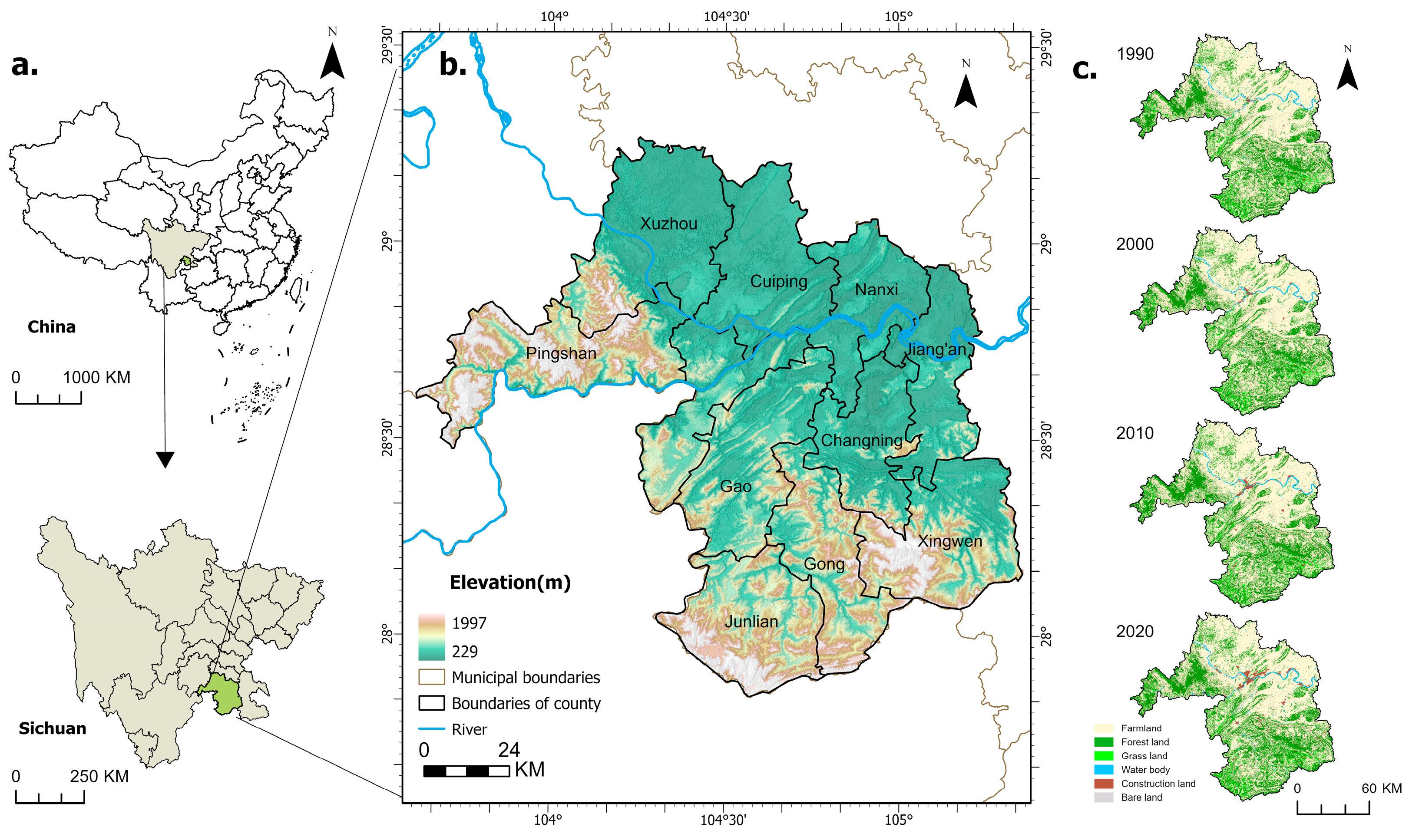
2.1. Study Area

Yibin City (27°50′–29°16′ N, 103°36′–105°20′ E) is located in the southeastern part of Sichuan Province (Figure 1). Covering a total area of 13,283 square kilometers, the city comprises three districts and seven counties. In recent years, Yibin has experienced rapid economic development, with a GDP growth rate that ranks among the highest in the country. Located in the upper reaches of the Yangtze River, with tributaries such as the Jinsha River and Min River flowing through its territory, the city boasts abundant water resources and serves as a crucial ecological barrier. The terrain is generally high in the southwest and low in the northeast, with an altitude of 229–1997 m. The landscape is dominated by low and medium mountains and hills, and certain southern regions feature karst topography. Yibin has a medium subtropical humid monsoon climate, with an average annual temperature of around 18 °C. The city receives an average annual precipitation ranging from 1050 to 1618 mm, with the rainy season occurring between May and October 2022, its forest coverage rate reaches 46.9%, and it is one of the top ten bamboo-resource-rich areas in the country and a typical area for returning farmland to bamboo. Previous studies have shown that the project has improved soil and water conservation capacity [29].

2.2. Data Sources and Description

The data used in this study cover many aspects of land use, topography, climate, vegetation, socio-economics, soil texture, etc., in Yibin City, and their sources and details are shown in

Table 1. Data sources.

Data	Data Formats	Time	Source
Land-use data	Raster (30 m)	1990, 2000, 2010, 2020	Resource and Environment Science and Data Center (www.resdc.cn/, accessed on 22 July 2023)
DEM	Raster (30 m)	2020	National Aeronautics and Space Administration (https://ladsweb.nascom.nasa.gov/search/, accessed on 15 June 2023)
Temperature data	Raster (1 km)	1990, 2000, 2010, 2020	The National Meteorological Science Data Center (http://data.cma.cn/, accessed on 19 July 2023)
Precipitation data
Fractional vegetation cover data	Raster (250 m)	1990, 2000, 2010, 2020	National Tibetan Plateau / Third Pole Environment Data Center (https://data.tpdc.ac.cn/, accessed on 25 July 2023)
GDP	Raster (1 km)	1990, 2000, 2010, 2020	Resource and Environment Science and Data Center (https://www.resdc.cn/, accessed on 22 August 2023)
Population distribution data
Boundary and road network data	Vector	2023	National Geographic Information Resource Catalogue Service System (https://www.webmap.cn/, accessed on 14 June 2023)
Depth to bedrock data	Raster (250 m)	2017	The Soil and Terrain Database (https://data.isric.org/, accessed on 3 August 2023)
Soil water capacity data
Soil sand content data

. The slope data were calculated by DEM. All the data were unified into the projected coordinate system (WGS_1984_UTM_Zone_48N).

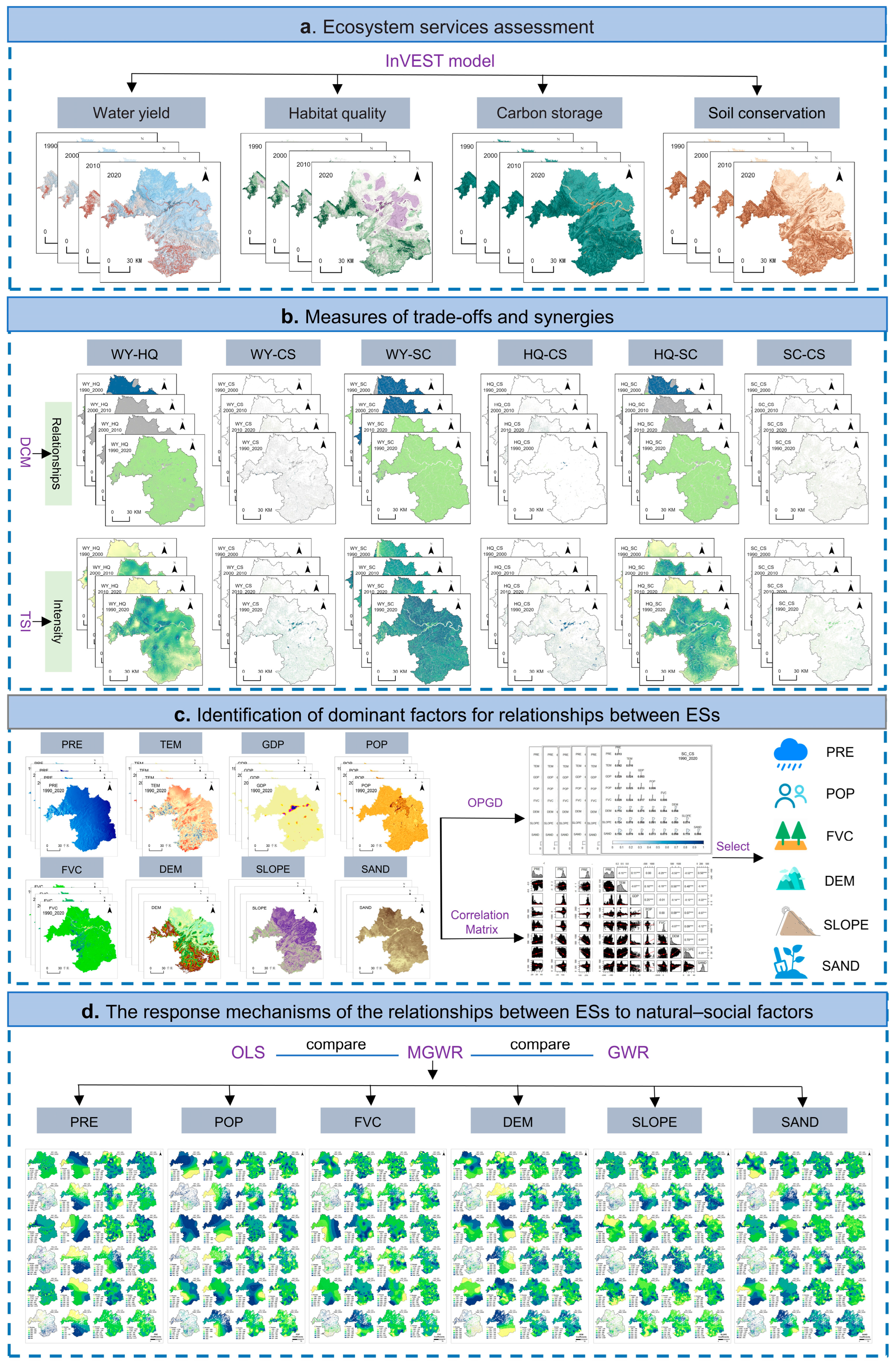
2.3. Assessment of Ecosystem Services

The methodological framework for the present study is presented in Figure 2. Four types of ESs are assessed using the InVEST model. This model considers most ecological processes and has been used by scholars all over the world. It has validated a large number of simulated values and measured values, making the parameter settings for different regions well justified. Its accuracy is relatively reliable.

2.3.1. Water Yield

The “Annual Water Yield” module of the InVEST model is based on the principle of water balance, and the water yield of pixel x is calculated using the following formula:

$$\mathrm{W}\mathrm{Y}=(1-\mathrm{A}\mathrm{E}\mathrm{T}/\mathrm{P})/\mathrm{P}$$

(1)

where AET refers to the actual evaporation, and P refers to the annual rainfall. The values of each parameter are taken from related studies [30,31]. The biophysical table is shown in Table S1. This study uses the three-year average rainfall and evaporation to calculate WY, thus reducing the impact of potential extreme values. Compared with the Yibin water resources bulletin (Table S2), the simulation accuracy in 2010 was 0.833, and in 2020, it was 0.920. The water resources bulletin before 2010 is missing.

2.3.2. Habitat Quality

We quantified HQ using the ‘Habitat quality’ module of InVEST. It calculates HQ by considering the intensity of external pressures from threat sources and the relative suitability of each land cover type for each threat. Threat sources include urban built-up land, rural settlements, roads of different classes, and railways [32]. The details are shown in Table S3. The HQ values can be expressed as follows:

$$\mathrm{H}\mathrm{Q}=\mathrm{H}\times \left\{1-(\mathrm{D}/\mathrm{D}+\mathrm{K})\right\}$$

(2)

where H refers to the habitat suitability score, D refers to the degree of habitat degradation, and K is the half-saturation constant.

2.3.3. Carbon Storage

We calculated CS using the “Carbon Storage and Sequestration” module of InVEST, which is based on land-use data and four carbon pools. The parameter settings mainly refer to previous scholars’ research on carbon storage in the Sichuan and Chongqing regions [33,34,35]. Detailed information can be found in Table S4. The following is the formula for calculating CS.

$$\mathrm{C}\mathrm{S}={\sum }_{i=0}^{\mathrm{n}}\mathrm{A}\times ({\mathrm{C}}_{\mathrm{a}\mathrm{b}\mathrm{o}\mathrm{v}\mathrm{e}}+{\mathrm{C}}_{\mathrm{b}\mathrm{e}\mathrm{l}\mathrm{o}\mathrm{w}}+{\mathrm{C}}_{\mathrm{s}\mathrm{o}\mathrm{i}\mathrm{l}}+{\mathrm{C}}_{\mathrm{d}\mathrm{e}\mathrm{a}\mathrm{d}})$$

(3)

where A refers to the land-use type; ${\mathrm{C}}_{\mathrm{a}\mathrm{b}\mathrm{o}\mathrm{v}\mathrm{e}}, {\mathrm{C}}_{\mathrm{b}\mathrm{e}\mathrm{l}\mathrm{o}\mathrm{w}}, {\mathrm{C}}_{\mathrm{s}\mathrm{o}\mathrm{i}\mathrm{l}}, \mathrm{a}\mathrm{n}\mathrm{d} {\mathrm{C}}_{\mathrm{d}\mathrm{e}\mathrm{a}\mathrm{d}}$ are carbon densities for aboveground biomass, belowground biomass, soil, and dead organic matter, respectively.

2.3.4. Soil Conservation

We used the “Sediment delivery ratio” module in InVEST to calculate SC. This module utilizes the Revised Universal Soil Loss Equation (RUSLE) and represents SC based on the difference between potential and actual soil loss. To more accurately simulate soil conservation, this paper divides farmland into six grades according to slope during calculation. The specific parameter settings can be found in Table S5 [36,37]. The calculation formula is as follows:

$$\mathrm{S}\mathrm{C}=\mathrm{R}\times \mathrm{K}\times \mathrm{L}\mathrm{S}\times (1-\mathrm{C}\times \mathrm{P})$$

(4)

R is the rainfall erosivity factor, K is the soil erodibility factor, LS is the slope length gradient factor, C is the vegetation-cover-management factor, and P is the soil-water conservation measures factor.

2.4. Measurement of Relationships between Ecosystem Services

2.4.1. Identification of Trade-Offs and Synergies between ESs

Zhang et al. proposed a method of difference comparison to determine the trade-off and synergy relationships between ESs [19]. But they ignored the distinction between positive and negative synergistic relationships. In this paper, an improved difference comparison method (DCM) is used to determine the trade-off relationship, positive synergistic relationship, and negative synergistic relationship between ESs. In order to have comparability between different ESs and at different periods, it is first standardized, and then, the change value of each ecosystem service is calculated after standardization at different periods, and finally, it is compared. This approach can visualize the spatial patterns of trade-offs and synergies and can be represented mathematically as follows:

$${STD\_ES}_{it}=\frac{{ES}_{it}-min\left({ES}_{t1},{ES}_{t2},\cdots \right)}{\max \left({ES}_{t1},{ES}_{t2},\cdots \right)-min\left({ES}_{t1},{ES}_{t2},\cdots \right)}$$

(5)

$$∆{ES}_i={STD\_ES}_{it2}-{STD\_ES}_{it1}$$

(6)

$$\left\{\begin{array}{l}∆{ES}_{Ai}>0 and ∆{ES}_{Bi}>0 \left(\mathrm{p}\mathrm{o}\mathrm{s}\mathrm{i}\mathrm{t}\mathrm{i}\mathrm{v}\mathrm{e} \mathrm{s}\mathrm{y}\mathrm{n}\mathrm{e}\mathrm{r}\mathrm{g}\mathrm{i}\mathrm{e}\mathrm{s}\right) \\ ∆{ES}_{Ai}<0 and ∆{ES}_{Bi}<0 \left(\mathrm{n}\mathrm{e}\mathrm{g}\mathrm{a}\mathrm{t}\mathrm{i}\mathrm{v}\mathrm{e} \mathrm{s}\mathrm{y}\mathrm{n}\mathrm{e}\mathrm{r}\mathrm{g}\mathrm{i}\mathrm{e}\mathrm{s}\right)\\ ∆{ES}_{Ai}<0 and ∆{ES}_{Bi}>0 \left( \mathrm{t}\mathrm{r}\mathrm{a}\mathrm{d}\mathrm{e}\mathrm{o}\mathrm{f}\mathrm{f}\mathrm{s} \right) \end{array}\right.$$

(7)

${STD\_ES}_{it}$ denotes the standardized value of ESs in the i-th grid at period t. $∆{ES}_{Ai}$ represents the change in value of type A ESs on the i-th grid after standardization from period t1 to t2.

2.4.2. Determination of the Intensity of Trade-Offs and Synergies between ESs

Xue et al. first proposed the trade-off–synergy index (TSI), which is based on the difference in changes in two ESs to calculate the intensity of their relationship [28]. However, this method may have problems distinguishing the magnitude of the intensity. This paper presents a modified trade-off–synergy index to quantify the intensity of trade-off and synergistic relationships. When one ES changes a lot and the other changes a little, their correlation is not strong, and we assume that the strength of their relationship is weak, while when their changes are similar, the strength of their relationship is stronger. Accordingly, this paper proposes TSI. It is a number between 0 and 1; the closer to 1, the stronger the trade-off or synergy, and vice versa. The index is expressed by the following formula:

$$\mathrm{T}\mathrm{S}\mathrm{I}=\frac{\sqrt{2\times \min \left[{\left(∆{ES}_{Ai}\right)}^2,{\left(∆{ES}_{Bi}\right)}^2\right]}}{\sqrt{{\left(∆{ES}_{Ai}\right)}^2+{\left(∆{ES}_{Bi}\right)}^2}}=\frac{\sqrt{2}\times min\left(∆{ES}_{Ai},∆{ES}_{Bi}\right)}{\sqrt{{\left(∆{ES}_{Ai}\right)}^2+{\left(∆{ES}_{Bi}\right)}^2}}$$

(8)

TSI is the ratio of the actual changes in ES_A and ES_B to the minimum changes among them. When the difference in changes in ES_A and ES_B is larger, the value is smaller, and when the changes are similar, the value is larger, which conforms to the definition of the strength of trade-off and synergy relationships. This method has stronger explainability and a clearer distinction of the strength of relationships.

2.5. Spatial Autocorrelation Analysis

2.5.1. Global Moran’s I

Moran’s I is a coefficient used to characterize the presence or absence of spatial autocorrelation [38]. Its values range from −1 to 1: a value of 1 signifies perfect positive spatial autocorrelation, 0 denotes spatial randomness, and −1 indicates perfect negative spatial autocorrelation. In this paper, we use the spatial autocorrelation tool of ArcGIS 10.8 to calculate Global Moran’s I to characterize the spatial autocorrelation of the intensity of trade-offs and synergies between ESs.

2.5.2. Hotspot Analysis

Hotspot analysis is a method that uses spatial autocorrelation to represent the relationship between a certain geographical attribute at a certain location and the same geographical attribute in the neighborhood [39]. The analysis results can reflect the positions of statistically significant hotspots or coldspots. In this study, the Getis-Ord Gi* statistic is employed to identify the hot and cold spots of the intensity of relationships between ESs.

2.6. Optimal Parameters-Based Geographical Detector Model and Drivers

Geographical detectors are a spatial statistical method for exploring spatially stratified heterogeneity and revealing the natural and anthropogenic processes behind it [40,41]. It can not only quantitatively measure the contribution of each driver to spatial heterogeneity but also determine the type and strength of the interaction between the two factors. The method has no linearity assumption and can be used without considering the existence of multicollinearity between data. The method of spatial data discretization and the determination of the number of classes are key aspects, which can be found in the Supplementary Materials. In previous studies, these parameters were generally based on empirical results, lacking precise quantitative evaluations. An optimal-parameter-based geographical detector calculates the results of different combinations of discretization methods and classification numbers and selects the optimal combination [42]. The q-statistic can be expressed by the following equation:

$$\mathrm{q}=1-\frac{{\sum }_{\mathrm{h}=1}^{\mathrm{L}}{\mathrm{N}}_{\mathrm{h}}{\mathsf{\sigma }}_{\mathrm{h}}^2}{{\mathrm{N}\mathsf{\sigma }}^2}$$

(9)

The value of q ranges from 0 to 1, and the closer it is to 1, the greater its explanatory power for the fractional anisotropy of the dependent variable. L is the stratification of all variables; N and ${\mathrm{N}}_{\mathrm{h}}$ are the total number of samples and the number of samples, respectively. The variables ${\mathsf{\sigma }}^2$ and ${\mathsf{\sigma }}_{\mathrm{h}}^2$ denote the variance within the study area and the dispersion variance of variable h within the sub-area, respectively.

Based on our field investigations and previous studies, a comprehensive selection of driving factors was made, encompassing five aspects: climate, socio-economics, vegetation, topography, and soil. These factors include precipitation (PRE), temperature (TEM), GDP, population distribution (POP), fractional vegetation cover (FVC), elevation (DEM), slope, and soil sand content (SAND) [25,43,44,45,46,47].

2.7. Multi-Scale Geographically Weighted Regression (MGWR)

Although the classical geographically weighted regression (GWR) introduces variable parameters compared to the global regression model, it presupposes that all modeled processes operate at the same spatial scale [48]. Fothering-ham et al. proposed multi-scale geographically weighted regression (MGWR) based on a generalized additive model [49]. This method allows each covariate to have its own spatial smoothing level, uses an optimal bandwidth for each independent variable in regression, and customizes the spatial scale at which each spatial process operates [50,51]. This results in spatial process models that are closer to reality and have greater explanatory power. In MGWR, the model can use the golden search algorithm to find the most suitable bandwidths for different variables for regression modelling, thus avoiding mismatches between the bandwidth and the scale of variable effects and reducing noise in parameter estimation. The formula for the model is as follows:

$$y_i={\sum }_{j=1}^k{\beta }_{bwj}\left(u_i,v_i\right)x_{ij}+{\epsilon }_i$$

(10)

where bwj represents the bandwidth used for the regression coefficient of the jth variable; $y_i$ represents the intensity of trade-offs and synergies between ESs in the ith grid. $x_{ij}$ denotes the jth built environment in the ith grid. $\left(u_i,v_i\right)$ denotes the centre of mass coordinates of the ith grid; ${\beta }_{bwj}$ denotes the regression coefficient of the jth variable in the ith grid under the bandwidth bwj; k denotes the sample size; and ${ \epsilon }_i$ denotes the random error term.

3. Results

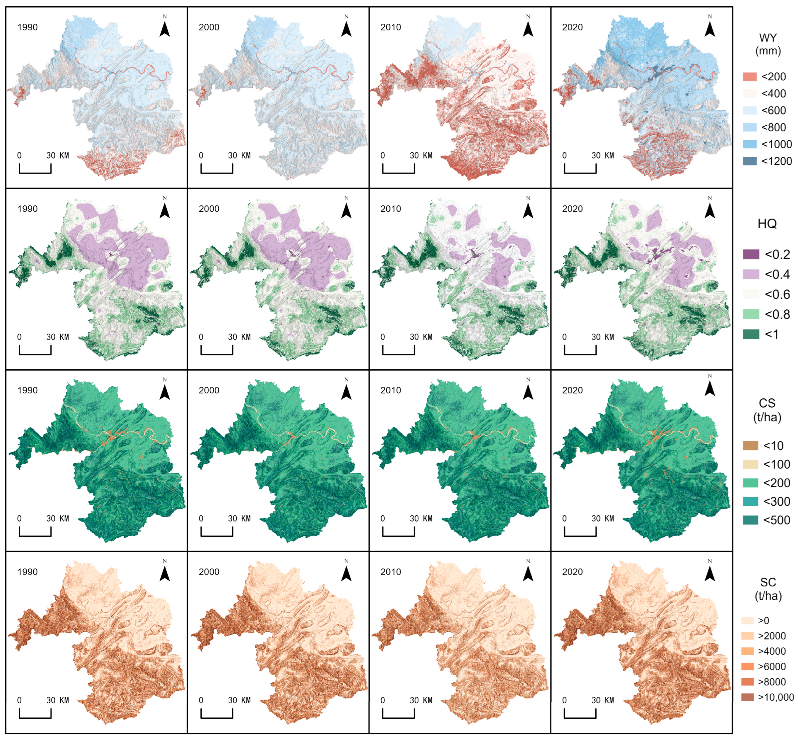
3.1. Characteristics of Spatial and Temporal Changes in Ecosystem Services

Over the thirty-year period from 1990 to 2020, various aspects such as the natural environment and socio-economics experienced different degrees of evolution. However, as seen from Figure 3, the spatial patterns of the ecosystem services HQ, CS, and SC remained stable, showing significant high–low clustering characteristics. Although WY consistently showed a pattern of low in the south and high in the north, the range of high and low distributions of its values showed significant changes in all periods. In terms of quantitative trends, all four ESs were in a fluctuating state. Specifically, the average provision of WY increased slightly from 412.56 mm in 1990 to 425.91 mm in 2000, then plummeted to 345.96 mm in 2010, and climbed again to 503.62 mm in 2020, reaching its highest value in the thirty-year span. In 1990, the area of low values of WY was mainly concentrated in the southwestern mountainous areas, while the other mountainous areas had a WY of about 300 mm, and the plains had values of about 500 mm. By 2000, the distribution of WY became more uniform and increased overall. By 2010, the WY supply had significantly reduced, with most high-altitude areas having values below 200 mm. In 2020, the distribution pattern of WY was similar to that of 1990, but its water yield had significantly increased, with more pronounced high–low clustering. The overall pattern change in WY can primarily be attributed to interannual rainfall fluctuations. On a local scale, the annual expansion of impervious surfaces has significantly contributed to the increase in local WY.

The range of HQ values is between 0 and 1, with higher values indicating better habitat quality. The average HQ declined from 0.5112 in 1990 to 0.5108 in 2000. During this period, rapid economic development led to a significant amount of construction land occupying agricultural land, thereby resulting in a decline in habitat quality. By 2010, as the GFGP was in full swing, with Yibin being a typical area for afforestation with bamboo, the HQ saw an increase of 3.7% that year, reaching 0.5470. In 2020, the GFGP ended, and some forest land was converted back to cropland. The area of construction land had approximately doubled compared to 2010. Consequently, the average HQ declined to 0.5416. From a spatial perspective, the HQ exhibited a pattern of being lower in the northeast and higher in the southern and northwestern parts. This spatial distribution can primarily be attributed to the gentle terrain in the northeast and the dominant land-use pattern being agricultural and construction land. Based on Figure 3, it is evident that the regions with an HQ value below 0.4 significantly decreased by 2010, further confirming the pivotal role of the GFGP in enhancing habitat quality.

The average capacity of CS decreased from 288.04 t/ha in 1990 to 287.79 t/ha in 2000. Between 2000 and 2010, the average capacity of CS increased by 0.15 t/ha due to the increase in forested land area. By 2020, the average capacity of CS decreased to 285.32 t/ha. It is worth noting that the CS in urban districts like Cuiping has been decreasing year by year. This is because the speed of urban expansion was the fastest in 2010–2020, resulting in a large encroachment on arable land. Additionally, during this period, the GFGP was also nearing its end. This indicates that the unordered expansion of construction land will exacerbate the decline in CS, which is unfavorable for China to achieve carbon neutrality. In comparison, between 1990 and 2000, the average capacity of SC increased from 5255.02 t/ha to 5464.47 t/ha, while in 2010, the mean SC plummeted by 1450.52 t/ha. This was mainly influenced by the significant decrease in precipitation in that year. By 2020, the mean capacity of SC increased to 6123.84 t/ha. This rising trend indicates that, under the comprehensive implementation of various soil and water conservation strategies such as converting steep slopes into terraces, significant progress has been made in controlling and improving soil erosion issues. The spatial patterns of CS and SC are both low in the northwest and high in the south and northeast, and both spatial patterns are stable. This is mainly attributed to the topography and the distribution pattern of forests and grasslands.

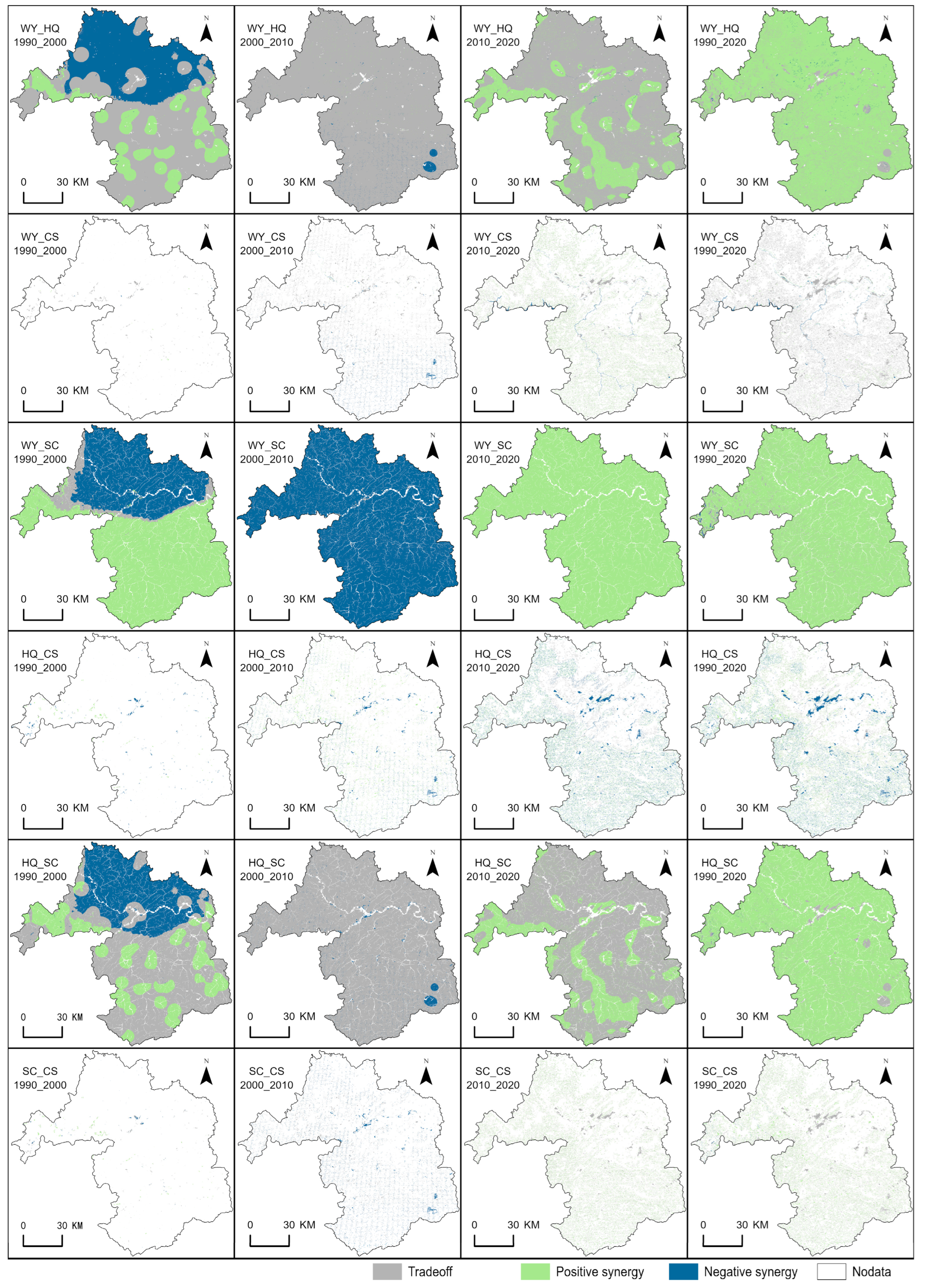
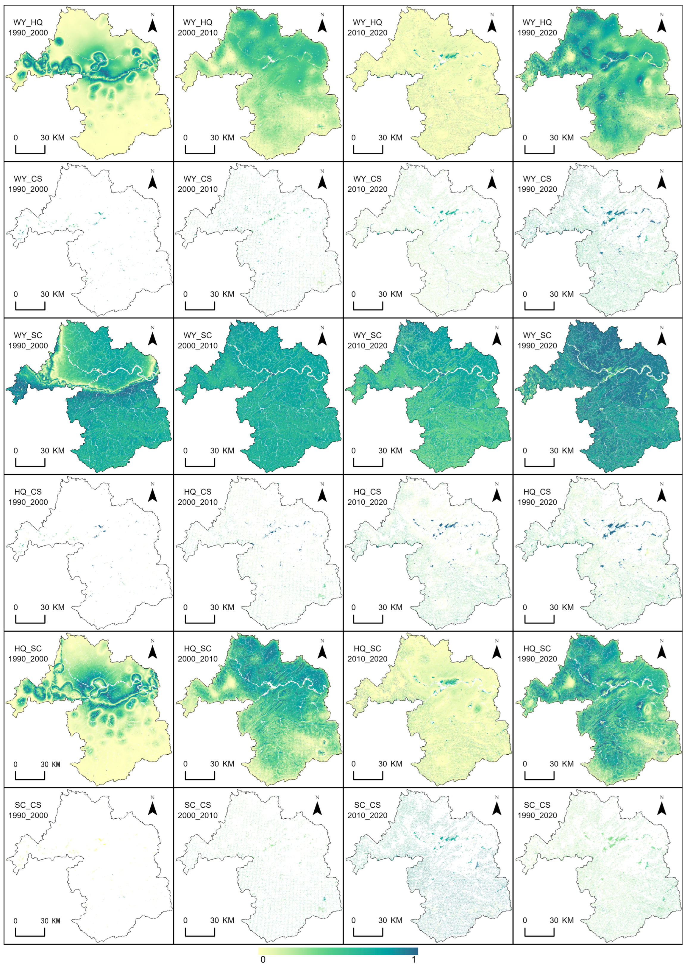
3.2. Spatial Patterns of Synergistic Ecosystem Service Trade-Offs

Figure 4 reveals the spatial distribution pattern of the trade-offs and synergies among the four ESs. Further, the TSI in Figure 5 quantifies the intensity of trade-offs and synergies among them. During the period 1990–2000, the trade-offs and synergies between WY and HQ were about equally divided, with a clear demarcation line in the region of 28°40′ N. North of this line, negative synergy relationships predominate, while south of this line, trade-off relationships prevail. During the period 2000–2010, WY and HQ were generally in a trade-off relationship, and the intensity was stronger than the previous decade. During this period, the implementation of the GFGP led to a significant increase in HQ. However, there was a substantial reduction in rainfall, leading to a decline in WY and a shift towards a trade-off relationship between the two. Areas with synergy were sporadically distributed, primarily in areas where land-use types posing less threat to habitat quality transitioned to more threatening land-use types, such as the conversion of farmland to construction land. Over the period 2010–2020, WY and HQ continued to be in an overall trade-off relationship, with a weakening of the strength of the trade-off in most of the region. Compared to the previous period, the areas of synergy increased, concentrated in regions where forest and water body areas expanded. Over the whole period, the whole region was dominated by strong synergy relationships, with the exception of building land where there were strong trade-offs. It is worth noting that there were strong trade-offs on some woodland and cropland in the south, which suggests the need to strengthen conservation measures to maintain and improve the overall quality of habitats.

In three periods and the entire period, trade-off relationships between WY and CS were mainly distributed on the construction land, and the intensity of trade-offs was increasing. In the second period, in the southern part, they mainly showed negative synergistic relationships. Especially in the southeast, there was a relatively large area of synergistic reduction. In this area, the forest land had been converted into grassland, and because of the reduction in rainfall, its carbon sequestration capability had declined. So, they presented a negative synergistic relationship. In the third period, many areas showed a positive synergistic relationship, which was mainly due to the increase in rainfall. It not only improves the water yield but also strengthens the carbon sequestration capability of vegetation.

During the period 1990–2000, there was an area of weak trade-offs between WY and SC in the middle region. In the north of this area, both had a negative synergy, while in the south, they increased synergistically. In the following period, their relationship across the entire region showed negative synergy, which decreased significantly in intensity. In contrast, the third period was entirely characterized by positive synergy, but its intensity was slightly lower than the previous period. In the whole period, their relationship was mainly one of positive synergy, with areas of trade-off being small and dispersed. This suggests that when changes in rainfall are substantial, WY and SC exhibit a synergistic relationship. The nature and intensity of their synergy primarily depend on the magnitude of increases or decreases in rainfall.

HQ and CS are closely related to forest and grass area. As the area of forest and grassland in a region expands, its carbon stock increases accordingly, and habitat quality also improves. Therefore, HQ and CS are positively correlated in most cases. From Figure 4, it can be observed that the two mainly show a negative synergy relationship in the study area during the three periods. The highest intensity of synergy is found in construction land. This does not indicate that construction land is favorable in promoting the synergy relationship between the two, but rather that both have decreased by the same amount. However, there are still areas that exhibit trade-offs, which are broadly categorized into two types. One type is where CS decreases while HQ increases, such as the conversion from farmland to water bodies. This change might enhance the ecological habitat quality, thereby favoring the survival of diverse flora and fauna. However, it might also affect the carbon sequestration capacity negatively. The other type is where CS increases while HQ decreases, for instance, in the conversion from farmland to economic forests. To facilitate transportation, roads might be constructed within the forested areas, leading to fragmentation of the forests. Although this transformation might increase the carbon stock, it could simultaneously decrease the habitat quality.

The distribution of trade-off and synergy relationships between SC and CS from 1990 to 2000 was quite scattered. In the second period, their synergy decreased, and the intensity of negative synergy in the central city area was high. Looking at the third period as well as the whole period, the trade-off relationships were concentrated in the urban area, and the intensity of trade-offs in the third period was the highest. In most of other areas, both showed positive synergistic relationships, with the third period having the highest degree of synergy. SC and CS exhibited a synergistic relationship from the perspective of ecological processes.

3.3. Spatial Autocorrelation Analysis for the Trade-Offs and Synergies between ESs

The spatial autocorrelation analyses of the trade-offs and synergies between four key ESs are shown in

Table 2. Spatial autocorrelation analysis of the trade-offs and synergies between ESs.

Type	Moran’s I	Z Score	p Value
WY_HQ 1990_2020	0.7727	173.3968	0.0000
WY_CS 1990_2020	0.3380	142.9039	0.0000
WY_SC 1990_2020	0.7414	166.4040	0.0000
HQ_CS 1990_2020	0.4688	198.1536	0.0000
HQ_SC 1990_2020	0.7790	174.8043	0.0000
SC_CS 1990_2020	0.3597	151.8130	0.0000

Abbreviation: WY: water yield; HQ: habitat quality; CS: carbon storage; SC: soil conservation.

. Results of the other three periods are shown in Table S6. All Moran’s I values are greater than 0, indicating that they are spatially positively correlated and show a significant clustering pattern, rather than being randomly or uniformly distributed.

Hotspot statistical analysis of relationships between ESs reveals their spatial and temporal distribution characteristics (Figure 6). In the first period, the hotspot region of the relationship strength between WY and HQ is mainly distributed around the dividing line of rainfall increase and decrease. In these areas, the change in rainfall is less, and its impact on WY and HQ is similar. In the second period, the hotspots are distributed in the plain area of the northeast, and the cold spots are distributed in the southern mountainous area, which may be related to the intensive human activities in the northeast. In the three periods, the relationship strength does not significantly dominate the entire area. Throughout the period, the proportions of hotspots and cold spots are roughly the same, with the former concentrated in the northwest and the latter in the southeast, which is mainly related to the distribution pattern of rainfall. As for WY and CS, in the first two periods, the hotspot regions are mainly distributed in the north, and the cold spot regions are distributed in the south. However, in the third period compared to the entire period, the distribution area of cold and hotspots is opposite, which is mainly related to the change pattern of rainfall. For WY and SC, the distribution of hot and cold spots in the first period lies on both sides of the line demarcating increased and decreased rainfall, with other regions being less significant. In other periods, hotspots are located in the northeastern region, while cold spots are in the southwest, potentially tied to the implementation of the GFGP since 1999, with significant positive effects on soil conservation in southern regions. With regard to HQ and CS, the spatial distribution of hot and cold spots is mirrored across different periods, showing spatial heterogeneity, possibly related to the distribution of vegetation types. The distribution patterns of cold and hotspots between HQ-SC and WY-HQ are akin. As for SC and CS, in the first two periods, hotspots are concentrated in the southern regions while cold spots in the north. This gradually shifts to hotspots in the east and cold spots in the west. Overall, the intensity of the relationship between the six pairs of ecosystem services presents a spatial distribution pattern of high and low clustering. However, the distribution pattern of hot and cold spots in each period is significantly different. This reveals the impact of time and space on their relationship.

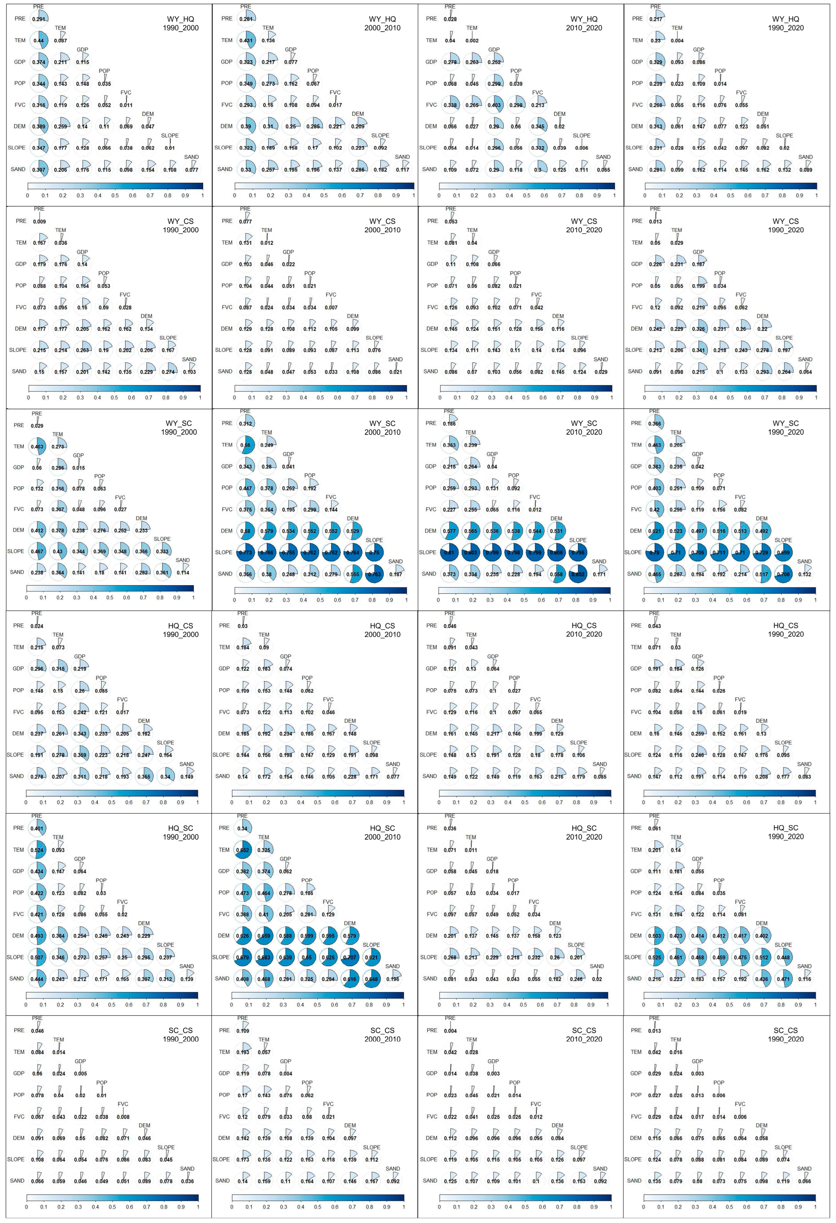
3.4. Identify the Dominant Factors for Trade-Offs and Synergies between ESs

As shown in Figure S1, the optimal discretization methods and classification numbers for different drivers of relationships between different ESs are different. However, most of the relationships between ESs have the highest q value with a classification number of 8. In terms of classification methods, the q value is highest when most driving factors choose natural breaks, quantile breaks, and geometric breaks.

The results of the factor detection and interaction detection of the OPGD are shown in Figure 7. They show that the dominant factors of the trade-offs and synergies between different ESs are different. And the dominant factors in the relationship between the same pair of ESs may also differ across different periods. Over the entire 30-year period, the relationship between WY and HQ was primarily influenced by precipitation, economic, and soil factors. This indicates that we can optimize the relationship between WY and HQ by adjusting economic models and improving soil. Most driving factors showed an increase in q values during the 2000–2010 period and a decrease during the 2010–2020 period. Notably, changes in topography and soil factors were pronounced. This was because the significant reduction in precipitation from 2000 to 2010 elevated the dominant role of soil and topographical characteristics in vegetation growth. In contrast, during the more rain-abundant period of 2010–2020, the influence of soil and topography factors relatively weakened, while the relationship became more influenced by precipitation. The relationship between WY and CS was mainly influenced by topographic, soil and economic factors, and it is noteworthy that the q value for soil sand content decreased from 0.103 to 0.029. This may be because high elevation and steep slopes promote the increase in both, while economic development significantly reduces carbon storage. Throughout the 30 years, precipitation, DEM, and slope played a dominant role in the changes in the intensity of relationship between WY and SC, with q-values of 0.366, 0.492, and 0.699, respectively. This is mainly because soil erosion primarily occurs in mountainous areas with abundant rainfall and steep slopes. This also indicates that this region is a key area for soil erosion control. The relationship between HQ and CS was more influenced by economic, topographic, and soil factors, with the main indicators including GDP, DEM, and soil sand content. This is mainly because both significantly decrease in high economic areas, while high elevation and fertile soil are conducive to a synergistic increase in both. Among the drivers of the relationship between HQ and SC, temperature and topographic factors had higher q-values than other factors. This may be because high temperatures affect vegetation growth. All eight drivers had low effects on the intensity of trade-offs and synergies between SC and CS, with slope having the highest q value of 0.074.

From the results of the interaction detection, it can be seen that there is a bi-factor enhancement or non-linear enhancement between all the drivers. This means that the joint effect of two drivers has a stronger effect on the response variable than a single factor. The influence of driving factor interactions on the response variable varies over time. For the relationship between WY and HQ, the joint effect of precipitation and temperature explains the highest value in the first and second period, shifting to GDP and FVC in the third period, with the combined effect of precipitation and GDP dominating throughout the 30-year period. The interaction of topography and other factors drives the intensity of trade-offs and synergies between WY and CS even more strongly, showing a strong driving effect in combinations with soil sand content, precipitation, FVC, and GDP, respectively, in different periods. For the relationship between WY and SC, the combined effect of precipitation and slope is more dominant in all the periods. The effect of the interaction of elevation and soil sand content is a stronger driver of the relationship between HQ and CS in the first period than the combination of the other drivers, shifting to GDP and elevation in other periods. The joint effect of precipitation and slope has stronger explanatory power for the relationship between HQ and SC. For the relationship between SC and CS, the effect of precipitation interacting with other drivers is more dominant. Interactive detection results also indicate that controlling several driving factors simultaneously is more effective in improving the relationships between ESs compared to controlling just one.

3.5. Diagnosis and Comparison of Models

OPGD reflects a non-linear relationship and reveals limited information, so we choose to compare OLS, GWR, and MGWR models. As shown in

Table 3. Comparison of the fitting measures for different models.

Type	OLS	GWR	MGWR
	Adj.R2	Adj.R2	Adj.R2
WY_HQ 1990_2020	0.2628	0.8248	0.8754
WY_CS 1990_2020	0.1195	0.5354	0.6180
WY_SC 1990_2020	0.3553	0.8537	0.8713
HQ_CS 1990_2020	0.1616	0.6542	0.7374
HQ_SC 1990_2020	0.5776	0.8661	0.9064
SC_CS 1990_2020	0.1356	0.4459	0.5164

Abbreviation: WY: water yield; HQ: habitat quality; CS: carbon storage; SC: soil conservation.

, the OLS model has the lowest r² value, while the MGWR model achieves the highest r² value. More details are shown in Table S7. This further confirms its superior performance in model fitting.

OLS, GWR, and MGWR are linear models that require a multicollinearity test on the independent variables before running. Typically, when the variation inflation factor (VIF) value exceeds 5, it indicates a moderate to high multicollinearity problem between the independent variables. When the OLS model was executed, the results showed that none of the VIF values for the respective variables exceeded 5. This demonstrated the relative independence of the data. If there is local multicollinearity among the independent variables, GWR model diagnostics cannot be obtained. To obtain a more precise comparison among the three models, the results from OPGD and the comprehensiveness of the driving factors were considered. Additionally, the correlation results of the driving factors were referenced (Figure S2), and a selection of independent variables was conducted. Given the local multicollinearity between GDP and several independent variables, it was excluded. There is local collinearity between temperature and precipitation. Combining the results of OPGD, rainfall has a higher explanatory power than temperature, so temperature was excluded. Finally, precipitation, population distribution, FVC, elevation, slope, and soil sand content were retained for further analysis.

We ran the MGWR model to explore the spatiotemporal differentiation of the impact of six driving factors on the trade-offs and synergies between ESs. As shown in Figure S3, most regional standardized residual values are between −2.5 and 2.5, indicating that the relationship between ESs and the independent variables is robust [19].

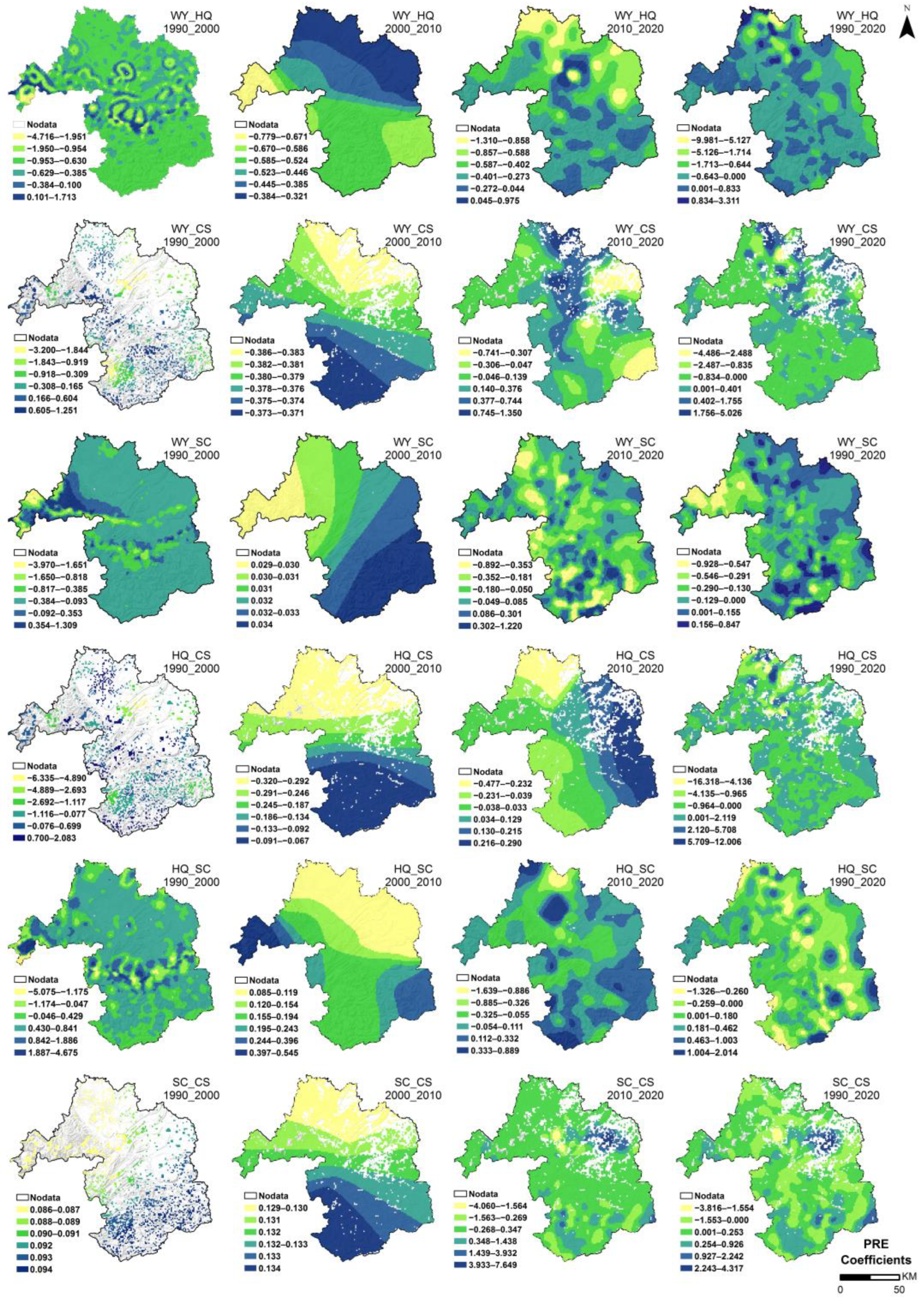
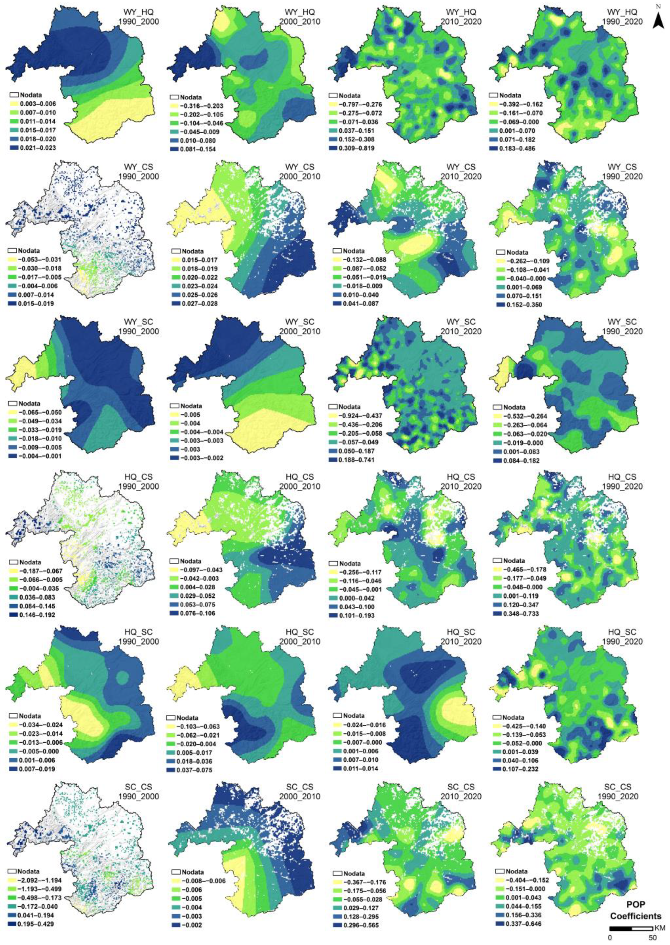
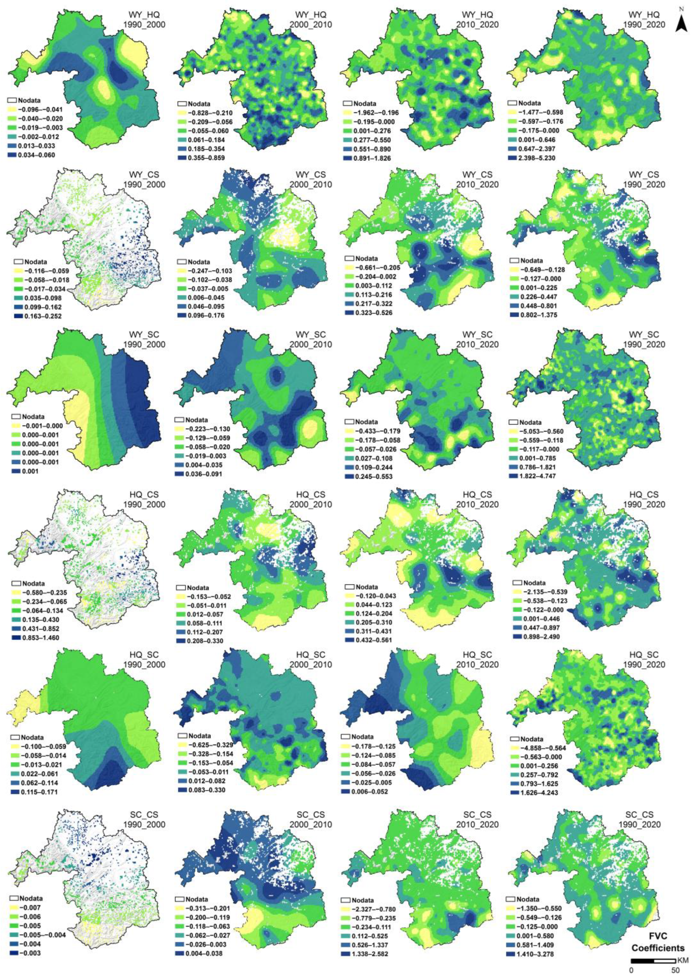
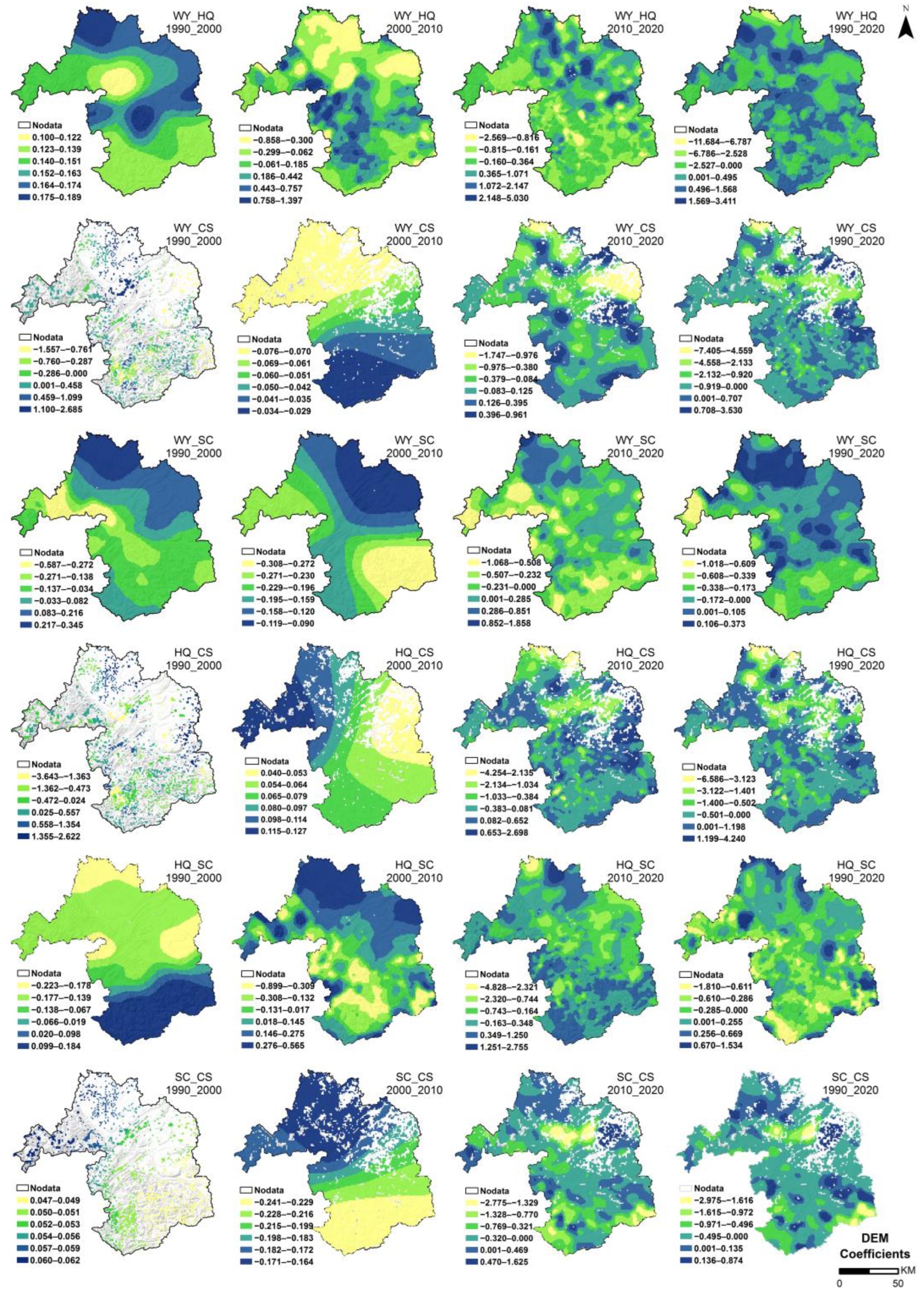
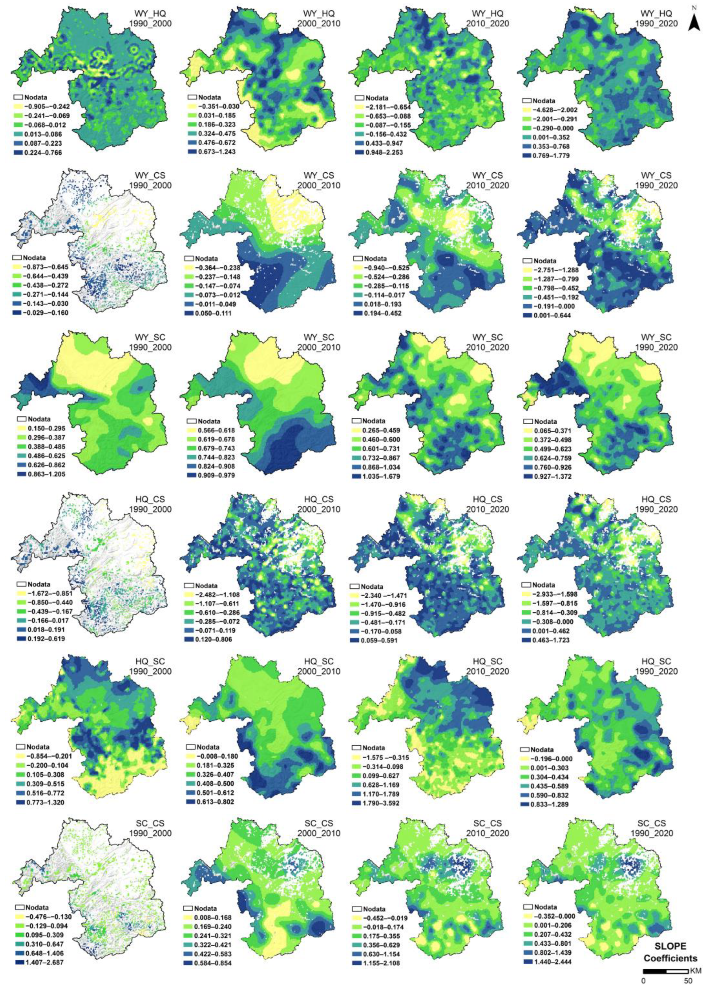
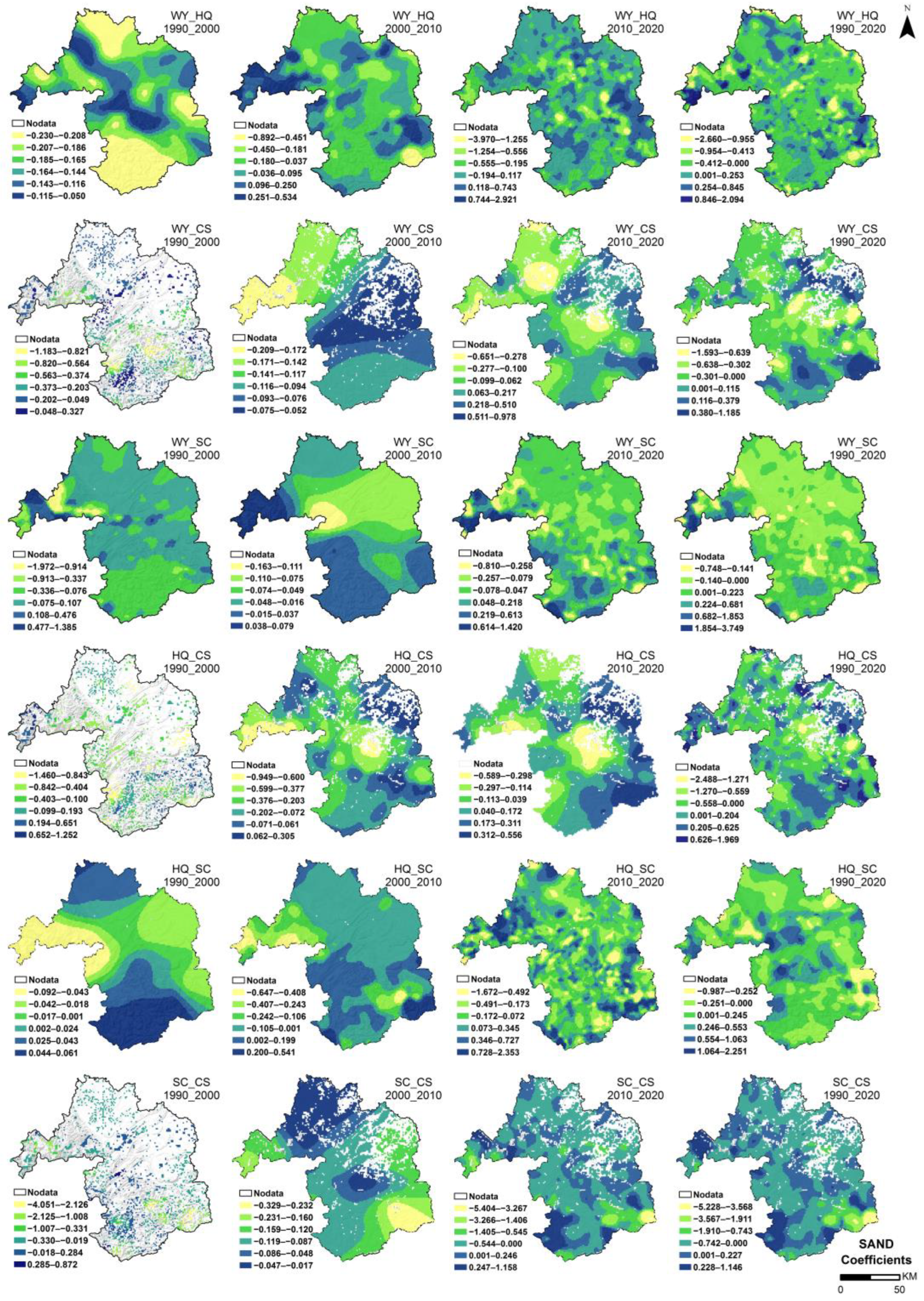
3.6. The Response Mechanisms of the Relationships between ESs to Natural–Social Factors

The MGWR coefficients for each driver in Figure 8, Figure 9, Figure 10, Figure 11, Figure 12 and Figure 13 reveal the spatial details of their contribution to the spatiotemporal differentiation in the intensity of trade-offs and synergies between ESs, which has important implications for the development of targeted and actionable ecological improvement actions.

The growth and development of plants and crops are regulated by a combination of climatic factors such as precipitation, temperature, and light, which in turn affect ESs and the relationships between them. The increase in climate extremes is threatening terrestrial carbon sinks, increasing the severity of soil water stress, and reducing biodiversity [52,53,54]. Precipitation plays an important role in climate change. Figure 8 depicts the extent to which changes in precipitation over time affect the relationship between ESs. In the first period, precipitation broadly shows a pattern of decreasing in the north and increasing in the south. In the second period, the extent of precipitation reduction increases from north to south, reflecting that the more the rainfall decreases, the lower the reduction in the trade-off intensity between WY and HQ. However, during this period, due to the implementation of the GFGP, the CS, HQ, and SC, which should decrease in areas with reduced rainfall, instead increase within the project area, thereby altering their relationships. In the third period and the entire period, the degree of precipitation increase intensifies from west to east. This change results in increased trade-offs between WY-HQ, and WY-CS, around the central urban area. Different plant species differ in their sensitivity, direction, and intensity of response to precipitation changes. The growth of plants in response to precipitation changes does not exhibit a linear relationship but rather display discontinuous threshold responses [55]. There are significant differences in threshold responses to precipitation among different land-use types and regions. Once the threshold range is exceeded, the responses shift in the opposite direction.

Managers can implement measures to reduce the losses of ESs due to climate stress. For instance, in rice ecosystems, adjusting the height of drainage outlets throughout the growth period can control drainage intensity, thereby improving the efficiency of rainfall utilization and achieving the maximum production–drainage ratio [56]. Moreover, the rainfall in Yibin is relatively abundant. In the southern mountainous areas, it is necessary to prevent geological disasters caused by soil erosion and other factors, so as to avoid exacerbating the trade-offs between SC and CS, as well as HQ.

Figure 9 shows the spatial details of the impact of population distribution on the trade-offs and synergies between ESs. Population migration and natural increase have shaped the pattern of population distribution.

In the first period, with the rise of the city, the central city attracts many people, while residents of the higher elevations migrate to the plains. In the second period, the central city continues to expand, leading to a decrease in population in the surrounding areas. In the third period, reverse urbanization occurs, and the population of the central city decreases. The response of the relationship between ESs to population distribution does not vary linearly, and different areas have different optimal population density ranges. Throughout the period, population growth is concentrated in parts of the southern and northwestern parts of the central urban area, with a general decrease in population in the counties surrounding the central urban area. An increase in the urban population has a positive effect on the strengthening of trade-off intensity between WY-HQ and WY-CS, as well as the negative synergistic intensity between HQ and CS, while it has a negative effect on the enhancement of the synergy between WY and SC and the trade-off intensity between HQ-SC and SC-CS. It is recommended that managers adopt policies to decentralize the population, such as offering incentives for population migration, to promote balanced regional economic development. Additionally, there is a need to enhance the technological level of agriculture, which can reduce unnecessary manual labor while also increasing the synergy between ESs. In certain forest areas, it may be suitable to develop eco-tourism, improve local forest management, and create eco-themed attractions similar to the “Shunan Bamboo Sea”. This not only helps to enhance the level of synergy between ESs but also increases income. Currently, the issue of talent outflow in Yibin City has been alleviated, and many young people are willing to work in Yibin. Attracting talent to work in various counties helps promote balanced development across different regions.

Figure 10 illustrates the spatial distribution of MGWR coefficients for FVC on the relationship between ESs. In the first period, the increase in vegetation cover was mainly located in the territory of Gao County, west of Yibin. In the second period, the whole area showed an increasing trend in vegetation cover, especially in the south. In the third period, the vegetation cover in the mountainous areas in the northwest increased significantly. In the whole period, the vegetation cover in Gao County increased most significantly, while the vegetation cover of the construction land distributed along the river decreased most significantly. The increase in FVC will obviously increase the values of CS and HQ, but the expansion of forest cover increases the demand for water resources, which may lead to the decrease in WY. Especially in the plains, the large-scale implementation of forest return may exacerbate the intensity of trade-off between ESs and may affect the growth of crops. Therefore, the GFGP should not be implemented on a large scale in the northeastern plain area of Yibin, as it may exacerbate the risk of drought. This is consistent with previous research conclusions [25,57]. The decline in vegetation coverage lowers the habitat quality that should naturally be high along riverbanks, reducing CS and SC values. At the same time, it also reduces vegetation water consumption, which may increase WY and thereby exacerbate the trade-off between them. The significant reduction in vegetation in urban areas not only intensifies the trade-offs among ESs but also exacerbates the urban heat island effect. Therefore, managers should promote an increase in the proportion of urban green spaces, enhancement of tree species diversity, and adoption of appropriate planting strategies [58,59]. In mountainous areas, the increase in vegetation coverage effectively prevents soil erosion, enhances SC, CS, and HQ [60], and promotes changes in soil structure, suppressing disasters such as landslides [61]. The pattern of water cycle in mountainous areas is not consistent with that of the plains, as lower temperatures and water vapor from vegetation transpiration make it easier for rain to fall in mountainous areas [62]. Moderately increasing vegetation coverage in mountainous areas can help increase WY, thereby enhancing the synergy among ESs. The Yibin City government should strive to expand the planting area of bamboo forests and vigorously develop the characteristic bamboo industry. This not only helps optimize ESs but also increases farmers’ income.

Figure 11 and Figure 12 show the distribution of MGWR coefficients for the effect of DEM and slope geomorphological factors on the relationship between ESs. Both slope and altitude show a trend of gradually increasing from northeast to southwest. It can be seen that there are differences in the direction and strength of the effect of geomorphological factors on the relationship between them in different periods. It can be observed that there is a trade-off region between HQ and SC in the southeast. In this region, the altitude and slope are relatively low compared to the surrounding areas.

The low slope enhances the trade-offs between the two, while the low altitude weakens it. The reduced slope decreases the risk of soil erosion but increases the likelihood of human activity interference, resulting in a decrease in both HQ and SC. SC is less sensitive to altitude compared to HQ, and HQ is more variable than SC, thus weakening the trade-off. In some areas of the southern mountainous region, both HQ and CS synergistically decrease. Although the characteristics of low temperature and high precipitation in high-altitude areas are conducive to carbon sequestration [63], the reduction in biological activity reduces pollination opportunities, leading to an overall decrease in CS and HQ. Moreover, temperature and precipitation differences on different slopes affect vegetation growth. Research has shown that in warm and dry areas, vegetation on the northern slope is better than that on the southern slope, while the opposite is true in cold and humid areas [64].

With urbanization, a large number of mountain populations in Yibin City have migrated to the northeastern plains, which has led to improvements in both the HQ and CS of the mountainous areas. The mountain population in Yibin City mostly resides at an altitude of around 1000 m. When the altitude surpasses the highest level of resident activities, issues such as soil erosion may worsen due to a lack of management. In addition, high altitudes are not conducive to pollination.

Soil texture varies in terms of soil fertility and water infiltration characteristics, which affects vegetation growth and ecosystem services [65]. Soil sand content is an important indicator of soil texture. The distribution of coefficients of its effect on the relationship between ESs is shown in Figure 13. The distribution of soil sand content is roughly in a pattern of high in the north and low in the south. In the south, good soil texture indicates its strong ability to conserve water and soil, which is conducive to vegetation growth. The higher SC in the south than in the north also proves this point. Most of the places with low soil sand content are forested or farmland, and their terrain is relatively gentle. In the southeast, there is an area where there is a trade-off between WY-HQ, HQ-SC, WY-CS, and SC-CS, while WY-SC are positive synergistic, and HQ-CS are negative synergistic. In this area, the soil sand content is obviously higher, which, to some extent, indicates that its soil texture is relatively poor. Good soil texture promotes the growth of vegetation, while the root system of plants improves the soil texture, and the interaction between the two changes the infiltration characteristics of the soil [66]. Thus, the HQ and CS decrease. The poor soil texture is more susceptible to erosion, so it may make SC increase. So, a high soil sand content enhances the trade-off between HQ-SC, and WY-CS, as well as the synergy between HQ-CS and WY-SC. In the south of Yibin, there are some karst areas with shallow soil layers and poor soil quality, which need to be improved by choosing suitable vegetation planting. At the same time, we can also learn from the “Xingwen Stone Sea” to build some special landscapes and invest the tourism income into improving the soil quality.

4. Discussion

4.1. Comparison of Related Studies and the Contribution of Generalization

This paper primarily explores the driving mechanisms of spatial heterogeneity in the trade-offs and synergies between ESs across different periods, with limited related studies available. Some scholars have conducted research on the relationships between different ESs in different regions using different methods. GDP, POP, and DEM promote the synergistic relationship between SC and outdoor recreation (OR) in the northern mountainous areas of Fujian Province. The expansion of construction land exacerbates the trade-off between OR and HQ in Fujian Province [19]. This is similar to our research findings. In the Yellow River Basin, climatic factors are gradually increasing the adverse effects on HQ, while reducing the promotion of food production (FP) and SC. Economic factors are also reducing the promotion of FP, but they have a certain positive effect on SC and WY [67]. This indicates that human intervention can help improve ecological problems caused by natural factors. In the Qinghai–Tibet Plateau, altitude and vegetation were the main factors influencing ES patterns in the early 20th century, but now temperature has replaced them as the primary factor [68]. This indicates that the impact of climate warming on highland ecosystems is becoming increasingly significant. In karst areas, there is a trade-off relationship between water conservation and SC, as well as net primary productivity (NPP), which is weakening. In addition, geological and climatic factors are the main factors influencing ESs [69]. From these studies, we can see that the dominant factors influencing the relationships among ESs vary across different regions. In mountainous areas, topographical and vegetation factors have a greater impact; in karst regions, lithology and slope factors are more significant; in urbanized areas, the negative effects of socio-economic factors are becoming increasingly apparent; in arid regions, climate is more likely to be the dominant factor. It is worth noting that different methods used to identify trade-off and synergy effects yield varying results.

Although the results obtained from different methods may be different, the systematic framework provided in this paper for exploring the mechanisms of trade-offs and synergies between ESs in different periods addresses the shortcomings of most related studies. The comparison of the results over multiple time periods makes the results more robust, so the framework is generalizable and can be used as a reference for other regions. First, this paper uses the idea of difference comparisons to identify trade-offs and synergies between ESs in a new dimension and quantifies the intensity of trade-offs and synergies between ESs spatially. Secondly, this paper identifies the dominant drivers and determines the strengths of the driver interactions through the OPGD. Finally, we explore how each driver in different regions affects the intensity of trade-offs and synergies between ESs across different periods using the MGWR model. Based on these findings, this study provides targeted suggestions for managers and also offers references for them in formulating sustainable development strategies. The data and models used in this paper are open-source, and the selection of driving factors is comprehensive and typical.

4.2. Suggestions for Achieving Sustainable Development of the Regional Ecological Environment

The goal of ES management is to effectively and fairly meet the preferences of stakeholders regarding ESs. Effectiveness refers to maximizing the benefits for the stakeholder group, while fairness refers to a relative balance of interests among stakeholders [70]. Currently, the main approaches to implementing ES management are through regulating land-use patterns and methods, adjusting land-use types, and multi-scenario multi-objective optimization measures. This article mainly provides some ecological management suggestions for different land-use types.

For construction land, it is necessary to regulate the development boundaries and urban form [71]. The development should shift from a single center to multiple centers, for example, the construction of Sanjiang New District. The transformation of old communities in Cuiping District should be undertaken, as well as control over the density and height of buildings in new urban areas, gradually shifting the population to county-level centers and villages. For transportation infrastructure projects such as the light rail in Yibin City, strict evaluation and approval should be conducted if it requires encroachment on arable land. And compensation should be provided by using more fertile land. It is more suitable for the construction of urban blue-green spaces in Yibin to concentrate on grasslands, small interconnected wetlands, and rows of trees [72]. These measures are conducive to the coordinated development of service and cultural services. As for cropland, fragmented and inefficient cropland should be rectified. The quantity of cropland should be increased, and the construction of high-standard farmland should be promoted. Young people should be attracted to engage in technology-oriented agriculture. Inter-cropping and rotation should be used to prevent soil erosion [73]. For cropland that is not suitable for cultivation, local characteristic programs (return farmland to bamboo) should be implemented, with certain compensation provided. Regarding forests and grasslands, reforestation and nature reserves should be encouraged in western and southern mountainous areas. The vegetation coverage in southern areas such as Xingwen County and Changning County, which are karst regions, should be increased to alleviate rocky desertification. Leisure natural attractions featuring bamboo forests and karst landscapes should be developed, so as to provide financial support for the protection of mountainous forests and grasslands. As for plain forests, conversion to cropland can be considered to improve the trade-off between WY and HQ and ensure food security. For water bodies, strict control over sewage discharge should be implemented to prevent eutrophication of water bodies. Wetland parks should be established along both sides of the river. River channels should be widened and the ecological environment restored to prevent flood disasters. In conclusion, implementing these measures is beneficial to improving the relationship between ESs.

4.3. Uncertainties and Directions for Future Work

This paper still has deficiencies and uncertainties. Firstly, the precision of each set of data is different, which could affect the ES pattern. Secondly, the InVEST model has its own shortcomings. On one hand, the determination of parameters is based on empirical values, leading to uncertainties. On the other hand, in the CS module, the CS value only changes when there is a shift in land-use types. However, in reality, the carbon storage can also vary due to factors such as climate and soil type. This discrepancy can result in biases between the trade-offs and synergies between CS and other ESs. Third, fewer ESs and drivers generated by human activities are selected, such as ESs of food production, recreation, and entertainment and drivers such as the area of GFGP. Fourth, this paper only identifies the trade-offs and synergies between the two ESs and their intensity, even though the multidimensional production frontier [74,75], cluster analyses [76] and PCA [77,78], and other methods have been used to determine the relationship between multiple ESs; however, the relationship between multiple ESs remains a difficult issue.

Future research directions should not only consider the trade-offs in supply but also consider trade-offs in demand as well as the balance between supply and demand. Exploring different geographical scales is also one of the key focuses of future research [67]. Furthermore, there is an urgent need to determine the threshold for the transition from trade-offs to synergies in the relationships between ESs, as well as to quantify the relationships between multiple ESs [79]. There are two important directions for future research on integrated ES applications. One is to couple geographical zoning with trade-offs in supply, trade-offs in supply and demand, and thresholds [80]. The other is to combine ecosystem service flows and ecological compensation from the perspectives of fairness and efficiency in the optimization of ESs [70].

5. Conclusions

(1) In this paper, the four key ESs in Yibin are assessed using the InVEST model, and the results show that with the acceleration of urbanization, the spatial distribution pattern of ESs has changed significantly in different periods, especially in the areas with more active urbanization. WY, CS, HQ, and SC show slight fluctuations over time, presenting a high–low clustering pattern in spatial distribution, with WY having the largest amplitude of change. It is obvious from the spatial pattern that there is spatial non-stationarity in the ESs.

(2) The methods of difference comparison and the trade-off–synergy index accurately measure the nature and intensity of the relationships between ESs spatially. The nature and intensity of their relationships have a high degree of spatial heterogeneity and temporal variability. The relationships among the four ESs are as follows: predominant positive synergies between WY-HQ, WY-SC, and HQ-CS, negative synergies between HQ and SC, and trade-offs between WY-CS and SC-CS. The intensity of the relationship between ESs in urban areas is high, while in other areas, it is relatively low. Overall, trade-off relationships dominate between ESs in the central urban area. So, managers need to focus the next step of ecological management on the central urban area.

(3) From the results of the identification of dominant factors, it can be seen that the intensity of the influence of each driver on the relationship between ESs varies in different periods: the relationship between WY and HQ is mainly affected by precipitation and the economy; the relationship between WY and CS is mainly affected by topography and soil; the relationship between WY and SC is mainly affected by precipitation and topography; the relationship between HQ and CS is mainly affected by economy and topography; the relationship between HQ and SC is mainly influenced by climate and topography factors; the relationship between SC and CS is mainly influenced by soil and topographic factors. In addition, the joint effect of the two drivers is stronger than the individual factors. It can be seen that the relationship between different ESs is influenced by different dominant factors, and the factors affecting the relationship between ESs are more complex and variable in the context of rapid urbanization.

(4) The MGWR model can help us better explore the driving mechanisms of various influencing factors on the changes in relationships between ESs. From the results, it can be observed that all driving factors may either improve or worsen the relationships between ESs. There exists a threshold, which varies for different land-use types and regions. Once this threshold is exceeded, the relationship will change in the opposite direction. The central urban area is the region where the trade-offs between ecosystem services are most prominent. Intensifying land use can lead to the establishment of more urban green spaces, controlling urban development boundaries and forms to minimize the fragmentation of ecological lands such as wetlands and forests. For farmland located on steep slopes or in areas with poor soil quality unsuitable for cultivation, the GFGP should continue to be implemented. At the same time, for forests and grasslands with tourism development potential, moderate and sustainable development is necessary.

In many regions, there are trade-offs among ESs, and uncertainties such as economic development and climate change are looming in the future. Improving the relationships between ESs is urgent. By combining the use of OPGD and MGWR, we can identify the dominant factors and driving mechanisms between ESs, and starting from these mechanisms, we can achieve a transformation from trade-offs to synergies. This framework can provide scientific support for ecological management in other regions.

References

1. Raudsepp-Hearne, C.; Peterson, G.D.; Bennett, E.M. Ecosystem service bundles for analyzing tradeoffs in diverse landscapes. Proc. Natl. Acad. Sci. USA 2010, 107, 5242–5247. [Google Scholar] [CrossRef] [PubMed]
2. Ricketts, T.H.; Regetz, J.; Steffan-Dewenter, I.; Cunningham, S.A.; Kremen, C.; Bogdanski, A.; Gemmill-Herren, B.; Greenleaf, S.S.; Klein, A.M.; Mayfield, M.M.; et al. Landscape effects on crop pollination services: Are there general patterns? Ecol. Lett. 2008, 11, 499–515. [Google Scholar] [CrossRef] [PubMed]
3. Bennett, E.M.; Peterson, G.D.; Gordon, L.J. Understanding relationships among multiple ecosystem services. Ecol. Lett. 2009, 12, 1394–1404. [Google Scholar] [CrossRef] [PubMed]
4. Chen, J.Y.; Jiang, B.; Bai, Y.; Xu, X.B.; Alatalo, J.M. Quantifying ecosystem services supply and demand shortfalls and mismatches for management optimisation. Sci. Total Environ. 2019, 650, 1426–1439. [Google Scholar] [CrossRef]
5. Yahdjian, L.; Sala, O.E.; Havstad, K.M. Rangeland ecosystem services: Shifting focus from supply to reconciling supply and demand. Front. Ecol. Environ. 2015, 13, 44–51. [Google Scholar] [CrossRef] [PubMed]
6. Ahern, J.; Cilliers, S.; Niemelä, J. The concept of ecosystem services in adaptive urban planning and design: A framework for supporting innovation. Landsc. Urban Plan. 2014, 125, 254–259. [Google Scholar] [CrossRef]
7. Goldstein, J.H.; Caldarone, G.; Duarte, T.K.; Ennaanay, D.; Hannahs, N.; Mendoza, G.; Polasky, S.; Wolny, S.; Daily, G.C. Integrating ecosystem-service tradeoffs into land-use decisions. Proc. Natl. Acad. Sci. USA 2012, 109, 7565–7570. [Google Scholar] [CrossRef] [PubMed]
8. Carpenter, S.R.; Mooney, H.A.; Agard, J.; Capistrano, D.; DeFries, R.S.; Díaz, S.; Dietz, T.; Duraiappah, A.K.; Oteng-Yeboah, A.; Pereira, H.M.; et al. Science for managing ecosystem services: Beyond the Millennium Ecosystem Assessment. Proc. Natl. Acad. Sci. USA 2009, 106, 1305–1312. [Google Scholar] [CrossRef] [PubMed]
9. Fang, L.; Liu, Y.; Li, C.; Cai, J. Spatiotemporal Characteristics and Future Scenario Simulation of the Trade-offs and Synergies of Mountain Ecosystem Services: A Case Study of the Dabie Mountains Area, China. Chin. Geogr. Sci. 2023, 33, 144–160. [Google Scholar] [CrossRef]
10. Tallis, H.; Kareiva, P.; Marvier, M.; Chang, A. An ecosystem services framework to support both practical conservation and economic development. Proc. Natl. Acad. Sci. USA 2008, 105, 9457–9464. [Google Scholar] [CrossRef]
11. Huang, Y.; Wu, J. Spatial and temporal driving mechanisms of ecosystem service trade-off/synergy in national key urban agglomerations: A case study of the Yangtze River Delta urban agglomeration in China. Ecol. Indic. 2023, 154, 110800. [Google Scholar] [CrossRef]
12. Chan, K.M.; Shaw, M.R.; Cameron, D.R.; Underwood, E.C.; Daily, G.C. Conservation planning for ecosystem services. PLoS Biol. 2006, 4, e379. [Google Scholar] [CrossRef] [PubMed]
13. He, J.; Shi, X.; Fu, Y.; Yuan, Y. Evaluation and simulation of the impact of land use change on ecosystem services trade-offs in ecological restoration areas, China. Land Use Policy 2020, 99, 105020. [Google Scholar] [CrossRef]
14. He, J.; Shi, X.; Fu, Y.; Yuan, Y. Spatiotemporal pattern of the trade-offs and synergies of ecosystem services after Grain for Green Program: A case study of the Loess Plateau, China. Environ. Sci. Pollut. Res. 2020, 27, 30020–30033. [Google Scholar] [CrossRef]
15. Li, T.; Ren, Y.; Ai, Z.; Qiao, Z.; Ren, Y.; Ma, L.; Yang, Y. Revealing the Spatial Interactions and Driving Factors of Ecosystem Services: Enlightenments under Vegetation Restoration. Land 2024, 13, 511. [Google Scholar] [CrossRef]
16. Chen, W.; Chi, G. Ecosystem services trade-offs and synergies in China, 2000–2015. Int. J. Environ. Sci. Technol. 2023, 20, 3221–3236. [Google Scholar] [CrossRef]
17. Zheng, H.; Peng, J.; Qiu, S.; Xu, Z.; Zhou, F.; Xia, P.; Adalibieke, W. Distinguishing the impacts of land use change in intensity and type on ecosystem services trade-offs. J. Environ. Manag. 2022, 316, 115206. [Google Scholar] [CrossRef] [PubMed]
18. Xu, S.; Liu, Y. Associations among ecosystem services from local perspectives. Sci. Total Environ. 2019, 690, 790–798. [Google Scholar] [CrossRef]
19. Zhang, Z.; Liu, Y.; Wang, Y.; Liu, Y.; Zhang, Y.; Zhang, Y. What factors affect the synergy and tradeoff between ecosystem services, and how, from a geospatial perspective? J. Clean. Prod. 2020, 257, 120454. [Google Scholar] [CrossRef]
20. Chen, T.; Peng, L.; Wang, Q. Response and multiscenario simulation of trade-offs/synergies among ecosystem services to the Grain to Green Program: A case study of the Chengdu-Chongqing urban agglomeration, China. Environ. Sci. Pollut. Res. 2022, 29, 33572–33586. [Google Scholar] [CrossRef]
21. Yuan, L.; Geng, M.; Li, F.; Xie, Y.; Tian, T.; Chen, Q. Spatiotemporal characteristics and drivers of ecosystem service interactions in the Dongting Lake Basin. Sci. Total Environ. 2024, 926, 172012. [Google Scholar] [CrossRef]
22. He, L.; Xie, Z.; Wu, H.; Liu, Z.; Zheng, B.; Wan, W. Exploring the interrelations and driving factors among typical ecosystem services in the Yangtze river economic Belt, China. J. Environ. Manag. 2024, 351, 119794. [Google Scholar] [CrossRef]
23. Tian, P.; Liu, Y.; Li, J.; Pu, R.; Cao, L.; Zhang, H. Spatiotemporal patterns of urban expansion and trade-offs and synergies among ecosystem services in urban agglomerations of China. Ecol. Indic. 2023, 148, 110057. [Google Scholar] [CrossRef]
24. Feng, Q.; Zhao, W.W.; Fu, B.J.; Ding, J.Y.; Wang, S. Ecosystem service trade-offs and their influencing factors: A case study in the Loess Plateau of China. Sci. Total Environ. 2017, 607, 1250–1263. [Google Scholar] [CrossRef] [PubMed]
25. Chen, T.Q.; Feng, Z.; Zhao, H.F.; Wu, K.N. Identification of ecosystem service bundles and driving factors in Beijing and its surrounding areas. Sci. Total Environ. 2020, 711, 134687. [Google Scholar] [CrossRef] [PubMed]
26. Liu, Y.; Yuan, X.; Li, J.; Qian, K.; Yan, W.; Yang, X.; Ma, X. Trade-offs and synergistic relationships of ecosystem services under land use change in Xinjiang from 1990 to 2020: A Bayesian network analysis. Sci. Total Environ. 2023, 858, 160015. [Google Scholar] [CrossRef] [PubMed]
27. Mansour, S.; Al Kindi, A.; Al-Said, A.; Al-Said, A.; Atkinson, P. Sociodemographic determinants of COVID-19 incidence rates in Oman: Geospatial modelling using multiscale geographically weighted regression (MGWR). Sustain. Cities Soc. 2021, 65, 102627. [Google Scholar] [CrossRef]
28. Xue, C.; Chen, X.; Xue, L.; Zhang, H.; Chen, J.; Li, D. Modeling the spatially heterogeneous relationships between tradeoffs and synergies among ecosystem services and potential drivers considering geographic scale in Bairin Left Banner, China. Sci. Total Environ. 2023, 855, 158834. [Google Scholar] [CrossRef]
29. Lu, H.-F.; Cai, C.-J.; Zeng, X.-S.; Campbell, D.E.; Fan, S.-H.; Liu, G.-L. Bamboo vs. crops: An integrated emergy and economic evaluation of using bamboo to replace crops in south Sichuan Province, China. J. Clean. Prod. 2018, 177, 464–473. [Google Scholar] [CrossRef]
30. Redhead, J.W.; Stratford, C.; Sharps, K.; Jones, L.; Ziv, G.; Clarke, D.; Oliver, T.H.; Bullock, J.M. Empirical validation of the InVEST water yield ecosystem service model at a national scale. Sci. Total Environ. 2016, 569–570, 1418–1426. [Google Scholar] [CrossRef]
31. Zhao, J.; Li, C. Investigating spatiotemporal dynamics and trade-off/synergy of multiple ecosystem services in response to land cover change: A case study of Nanjing city, China. Environ. Monit. Assess. 2020, 192, 701. [Google Scholar] [CrossRef] [PubMed]
32. Zhu, C.; Zhang, X.; Zhou, M.; He, S.; Gan, M.; Yang, L.; Wang, K. Impacts of urbanization and landscape pattern on habitat quality using OLS and GWR models in Hangzhou, China. Ecol. Indic. 2020, 117, 106654. [Google Scholar] [CrossRef]
33. Xiang, S.; Wang, Y.; Deng, H.; Yang, C.; Wang, Z.; Gao, M. Response and multi-scenario prediction of carbon storage to land use/cover change in the main urban area of Chongqing, China. Ecol. Indic. 2022, 142, 109205. [Google Scholar] [CrossRef]
34. Wang, C.D.; Li, T.Z.; Guo, X.H.; Xia, L.L.; Lu, C.D.; Wang, C.B. Plus-InVEST Study of the Chengdu-Chongqing Urban Agglomeration’s Land-Use Change and Carbon Storage. Land 2022, 11, 1617. [Google Scholar] [CrossRef]
35. Xiang, M.; Wang, C.; Tan, Y.; Yang, J.; Duan, L.; Fang, Y.; Li, W.; Shu, Y.; Liu, M. Spatio-temporal evolution and driving factors of carbon storage in the Western Sichuan Plateau. Sci. Rep. 2022, 12, 8114. [Google Scholar] [CrossRef] [PubMed]
36. Borji, M.; Samani, A.N.; Rashidi, S.; Tiefenbacher, J.P. Catchment-scale soil conservation: Using climate, vegetation, and topo-hydrological parameters to support decision making and implementation. Sci. Total Environ. 2020, 712, 136124. [Google Scholar] [CrossRef]
37. Xiao, Q.; Hu, D.; Xiao, Y. Assessing changes in soil conservation ecosystem services and causal factors in the Three Gorges Reservoir region of China. J. Clean. Prod. 2017, 163, S172–S180. [Google Scholar] [CrossRef]
38. Moran, P.P.A. The Interpretation of Statistical Maps. R. Stat. Soc. 1948, 10, 243–251. [Google Scholar] [CrossRef]
39. Liu, J.; Pei, X.; Zhu, W.; Jiao, J. Scenario modeling of ecosystem service trade-offs and bundles in a semi-arid valley basin. Sci. Total Environ. 2023, 896, 166413. [Google Scholar] [CrossRef]
40. Wang, J.F.; Zhang, T.L.; Fu, B.J. A measure of spatial stratified heterogeneity. Ecol. Indic. 2016, 67, 250–256. [Google Scholar] [CrossRef]
41. Wang, J.F.; Xu, C.D. Geodetector: Principle and prospective. Acta Geogr. Sin. 2017, 72, 116–134. [Google Scholar] [CrossRef]
42. Song, Y.Z.; Wang, J.F.; Ge, Y.; Xu, C.D. An optimal parameters-based geographical detector model enhances geographic characteristics of explanatory variables for spatial heterogeneity analysis: Cases with different types of spatial data. GISci. Remote Sens. 2020, 57, 593–610. [Google Scholar] [CrossRef]
43. Hu, C.; Wang, Z.; Li, J.; Liu, H.; Sun, D. Quantifying the Temporal and Spatial Patterns of Ecosystem Services and Exploring the Spatial Differentiation of Driving Factors: A Case Study of Sichuan Basin, China. Front. Environ. Sci. 2022, 10, 927818. [Google Scholar] [CrossRef]
44. Sun, X.Y.; Shan, R.F.; Liu, F. Spatio-temporal quantification of patterns, trade-offs and synergies among multiple hydrological ecosystem services in different topographic basins. J. Clean. Prod. 2020, 268, 122338. [Google Scholar] [CrossRef]
45. Haines-Young, R.; Potschin, M.; Kienast, F. Indicators of ecosystem service potential at European scales: Mapping marginal changes and trade-offs. Ecol. Indic. 2012, 21, 39–53. [Google Scholar] [CrossRef]
46. Niu, L.; Shao, Q.; Ning, J.; Huang, H. Ecological changes and the tradeoff and synergy of ecosystem services in western China. J. Geogr. Sci. 2022, 32, 1059–1075. [Google Scholar] [CrossRef]
47. Xu, S.N.; Liu, Y.F.; Wang, X.; Zhang, G.X. Scale effect on spatial patterns of ecosystem services and associations among them in semi-arid area: A case study in Ningxia Hui Autonomous Region, China. Sci. Total Environ. 2017, 598, 297–306. [Google Scholar] [CrossRef] [PubMed]
48. Brunsdon, C.; Fotheringham, A.S.; Charlton, M.E. Geographically Weighted Regression: A Method for Exploring Spatial Nonstationarity. Geogr. Anal. 1996, 28, 281–298. [Google Scholar] [CrossRef]
49. Fotheringham, A.S.; Yang, W.; Kang, W. Multiscale Geographically Weighted Regression (MGWR). Ann. Am. Assoc. Geogr. 2017, 107, 1247–1265. [Google Scholar] [CrossRef]
50. Hu, J.Y.; Zhang, J.X.; Li, Y.Q. Exploring the spatial and temporal driving mechanisms of landscape patterns on habitat quality in a city undergoing rapid urbanization based on GTWR and MGWR: The case of Nanjing, China. Ecol. Indic. 2022, 143, 109333. [Google Scholar] [CrossRef]
51. Wang, X.L.; Shi, S.H.; Zhao, X.; Hu, Z.R.; Hou, M.; Xu, L. Detecting Spatially Non-Stationary between Vegetation and Related Factors in the Yellow River Basin from 1986 to 2021 Using Multiscale Geographically Weighted Regression Based on Landsat. Remote Sens. 2022, 14, 6276. [Google Scholar] [CrossRef]
52. Bellard, C.; Bertelsmeier, C.; Leadley, P.; Thuiller, W.; Courchamp, F. Impacts of climate change on the future of biodiversity. Ecol. Lett. 2012, 15, 365–377. [Google Scholar] [CrossRef] [PubMed]
53. Knapp, A.K.; Beier, C.; Briske, D.D.; Classen, A.T.; Luo, Y.; Reichstein, M.; Smith, M.D.; Smith, S.D.; Bell, J.E.; Fay, P.A.; et al. Consequences of More Extreme Precipitation Regimes for Terrestrial Ecosystems. Bioscience 2008, 58, 811–821. [Google Scholar] [CrossRef]
54. Wolf, S.; Paul-Limoges, E. Drought and heat reduce forest carbon uptake. Nat. Commun. 2023, 14, 6217. [Google Scholar] [CrossRef] [PubMed]
55. Porter, J.R.; Semenov, M.A. Crop responses to climatic variation. Phil. Trans. R. Soc. B 2005, 360, 2021–2035. [Google Scholar] [CrossRef] [PubMed]
56. Gao, S.-K. Effect of Different Controlled Irrigation and Drainage Regimes on Crop Growth and Water Use in Paddy Rice. Int. J. Agric. Biol. 2018, 20, 486–492. [Google Scholar] [CrossRef]
57. Chen, L.; Pei, S.; Liu, X.N.; Qiao, Q.; Liu, C.L. Mapping and analysing tradeoffs, synergies and losses among multiple ecosystem services across a transitional area in Beijing, China. Ecol. Indic. 2021, 123, 107329. [Google Scholar] [CrossRef]
58. Jia, S.Q.; Wang, Y.H. Effect of heat mitigation strategies on thermal environment, thermal comfort, and walkability: A case study in Hong Kong. Build. Environ. 2021, 201, 107988. [Google Scholar] [CrossRef]
59. Wang, X.J.; Dallimer, M.; Scott, C.E.; Shi, W.T.; Gao, J.X. Tree species richness and diversity predicts the magnitude of urban heat island mitigation effects of greenspaces. Sci. Total Environ. 2021, 770, 145211. [Google Scholar] [CrossRef]
60. Li, W.; Chen, X.; Zheng, J.; Zhang, F.; Yan, Y.; Hai, W.; Han, C.; Liu, L. A Multi-Scenario Simulation and Dynamic Assessment of the Ecosystem Service Values in Key Ecological Functional Areas: A Case Study of the Sichuan Province, China. Land 2024, 13, 468. [Google Scholar] [CrossRef]
61. Fan, L.F.; Lehmann, P.; Zheng, C.M.; Or, D. Vegetation-Promoted Soil Structure Inhibits Hydrologic Landslide Triggering and Alters Carbon Fluxes. Geophys. Res. Lett. 2022, 49, 100389. [Google Scholar] [CrossRef]
62. Cui, J.P.; Lian, X.; Huntingford, C.; Gimeno, L.; Wang, T.; Ding, J.Z.; He, M.Z.; Xu, H.; Chen, A.P.; Gentine, P.; et al. Global water availability boosted by vegetation-driven changes in atmospheric moisture transport. Nat. Geosci. 2022, 15, 982–988. [Google Scholar] [CrossRef]
63. Xie, Y.; Lei, X.; Shi, J. Impacts of climate change on biological rotation of Larix olgensis plantations for timber production and carbon storage in northeast China using the 3-PGmix model. Ecol. Modell. 2020, 435, 109267. [Google Scholar] [CrossRef]
64. Yin, G.; Yan, X.; Ma, D.; Xie, J.; Chen, R.; Pan, H.; Zhao, W.; Wang, C.; Verger, A.; Descals, A.; et al. Polar-facing slopes showed stronger greening trend than equatorial-facing slopes in Tibetan plateau grasslands. Agric. For. Meteorol. 2023, 341, 109698. [Google Scholar] [CrossRef]
65. Ma, S.; Wang, L.-J.; Zhao, Y.-G.; Jiang, J. Coupling effects of soil and vegetation from an ecosystem service perspective. CATENA 2023, 231, 107354. [Google Scholar] [CrossRef]
66. Wang, P.P.; Su, X.M.; Zhou, Z.C.; Wang, N.; Liu, J.; Zhu, B.B. Differential effects of soil texture and root traits on the spatial variability of soil infiltrability under natural revegetation in the Loess Plateau of China. CATENA 2023, 220, 106693. [Google Scholar] [CrossRef]
67. Liu, Q.; Qiao, J.; Li, M.; Huang, M. Spatiotemporal heterogeneity of ecosystem service interactions and their drivers at different spatial scales in the Yellow River Basin. Sci. Total Environ. 2024, 908, 168486. [Google Scholar] [CrossRef]
68. Li, G.Y.; Jiang, C.H.; Gao, Y.; Du, J. Natural driving mechanism and trade-off and synergy analysis of the spatiotemporal dynamics of multiple typical ecosystem services in Northeast Qinghai-Tibet Plateau. J. Clean. Prod. 2022, 374, 134075. [Google Scholar] [CrossRef]
69. Li, Y.; Luo, H.F. Trade-off/synergistic changes in ecosystem services and geographical detection of its driving factors in typical karst areas in southern China. Ecol. Indic. 2023, 154, 110811. [Google Scholar] [CrossRef]
70. Su, B.; Liu, M. How to manage the ecosystem services effectively and fairly? J. Clean. Prod. 2024, 458, 142477. [Google Scholar] [CrossRef]
71. Liu, X.; Ming, Y.; Liu, Y.; Yue, W.; Han, G. Influences of landform and urban form factors on urban heat island: Comparative case study between Chengdu and Chongqing. Sci. Total Environ. 2022, 820, 153395. [Google Scholar] [CrossRef]
72. Lin, J.; Qiu, S.; Tan, X.; Zhuang, Y. Measuring the relationship between morphological spatial pattern of green space and urban heat island using machine learning methods. Build. Environ. 2023, 228, 109910. [Google Scholar] [CrossRef]
73. Sharpley, A.; Wang, X. Managing agricultural phosphorus for water quality: Lessons from the USA and China. J. Environ. Sci. 2014, 26, 1770–1782. [Google Scholar] [CrossRef] [PubMed]
74. Ruijs, A.; Wossink, A.; Kortelainen, M.; Alkemade, R.; Schulp, C.J.E. Trade-off analysis of ecosystem services in Eastern Europe. Ecosyst. Serv. 2013, 4, 82–94. [Google Scholar] [CrossRef]
75. Zhao, T.; Pan, J. Ecosystem service trade-offs and spatial non-stationary responses to influencing factors in the Loess hilly-gully region: Lanzhou City, China. Sci. Total Environ. 2022, 846, 157422. [Google Scholar] [CrossRef] [PubMed]
76. Lee, H.; Lautenbach, S. A quantitative review of relationships between ecosystem services. Ecol. Indic. 2016, 66, 340–351. [Google Scholar] [CrossRef]
77. Egarter Vigl, L.; Schirpke, U.; Tasser, E.; Tappeiner, U. Linking long-term landscape dynamics to the multiple interactions among ecosystem services in the European Alps. Landsc. Ecol. 2016, 31, 1903–1918. [Google Scholar] [CrossRef]
78. Zhu, Z.; Li, B.; Zhao, Y.; Zhao, Z.; Chen, L. Socio-Economic Impact Mechanism of Ecosystem Services Value, a PCA-GWR Approach. Pol. J. Environ. Stud. 2021, 30, 977–986. [Google Scholar] [CrossRef]
79. Zhao, M.; Zhou, Q.; Luo, Y.; Li, Y.; Wang, Y.; Yuan, E. Threshold Effects between Ecosystem Services and Natural and Social Drivers in Karst Landscapes. Land 2024, 13, 691. [Google Scholar] [CrossRef]
80. Wu, J.; Guo, X.; Zhu, Q.; Guo, J.; Han, Y.; Zhong, L.; Liu, S. Threshold effects and supply-demand ratios should be considered in the mechanisms driving ecosystem services. Ecol. Indic. 2022, 142, 109281. [Google Scholar] [CrossRef]
Figure 1. Overview of the study area: (a) location, (b) elevation and administrative units, (c) land use/cover.
Land 13 01009 g001
Figure 2. Research framework (WY: water yield; HQ: habitat quality; CS: carbon storage; SC: soil conservation; DCM: difference comparison method; TSI: trade-off–synergy index; PRE: precipitation; TEM: temperature; POP: population distribution; FVC: fractional vegetation cover; SAND: soil sand content).
Land 13 01009 g002
Figure 3. Spatial distribution patterns of the four key ecosystem services, 1990–2020 (WY: water yield; HQ: habitat quality; CS: carbon storage; SC: soil conservation).
Land 13 01009 g003
Figure 4. Spatial distribution of the trade-offs and synergies between the ESs (WY: water yield; HQ: habitat quality; CS: carbon storage; SC: soil conservation).
Land 13 01009 g004
Figure 5. Spatial distribution of the intensity of trade-offs and synergies between the ESs (WY: water yield; HQ: habitat quality; CS: carbon storage; SC: soil conservation).
Land 13 01009 g005
Figure 6. Spatial distribution of hotspots of trade-offs and synergies between ESs (WY: water yield; HQ: habitat quality; CS: carbon storage; SC: soil conservation).
Land 13 01009 g006
Figure 7. q-values of the drivers on the relationships between different ESs and the strength of the interactions (WY: water yield; HQ: habitat quality; CS: carbon storage; SC: soil conservation).
Land 13 01009 g007
Figure 8. The quantitative impact of precipitation in depicting trade-offs and synergies between ESs (WY: water yield; HQ: habitat quality; CS: carbon storage; SC: soil conservation).
Land 13 01009 g008
Figure 9. The quantitative impact of population distribution in depicting trade-offs and synergies between ESs (WY: water yield; HQ: habitat quality; CS: carbon storage; SC: soil conservation).
Land 13 01009 g009
Figure 10. The quantitative impact of fractional vegetation cover in depicting trade-offs and synergies between ESs (WY: water yield; HQ: habitat quality; CS: carbon storage; SC: soil conservation).
Land 13 01009 g010
Figure 11. The quantitative impact of DEM in depicting trade-offs and synergies between ESs (WY: water yield; HQ: habitat quality; CS: carbon storage; SC: soil conservation).
Land 13 01009 g011
Figure 12. The quantitative impact of slope in depicting trade-offs and synergies between ESs (WY: water yield; HQ: habitat quality; CS: carbon storage; SC: soil conservation).
Land 13 01009 g012
Figure 13. The quantitative impact of soil sand content in depicting trade-offs and synergies between ESs (WY: water yield; HQ: habitat quality; CS: carbon storage; SC: soil conservation).
Land 13 01009 g013