


Machine Learning-Driven Landslide Susceptibility Mapping in the Himalayan China–Pakistan Economic Corridor Region

 ,
, 
Abstract
1. Introduction
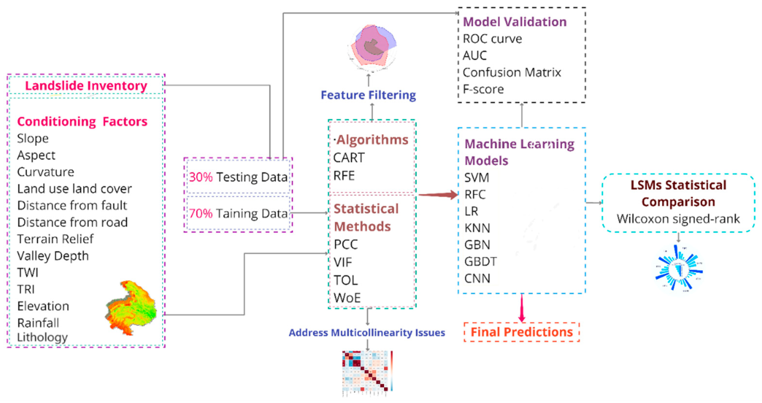
2. Materials and Methods
2.1. Study Area
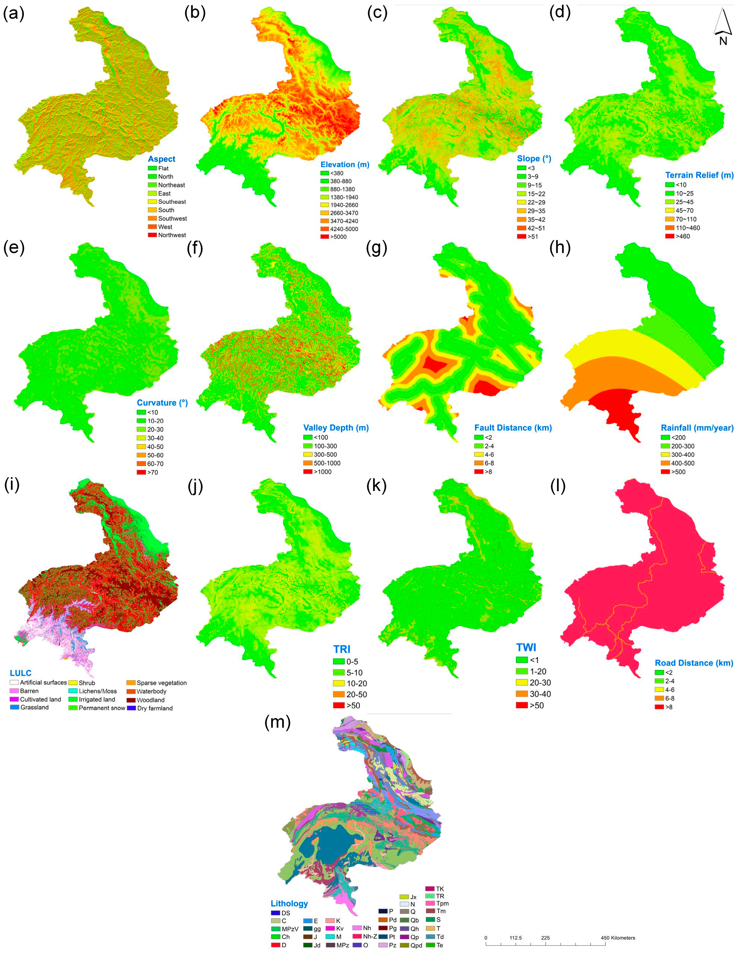
2.2. Datasets
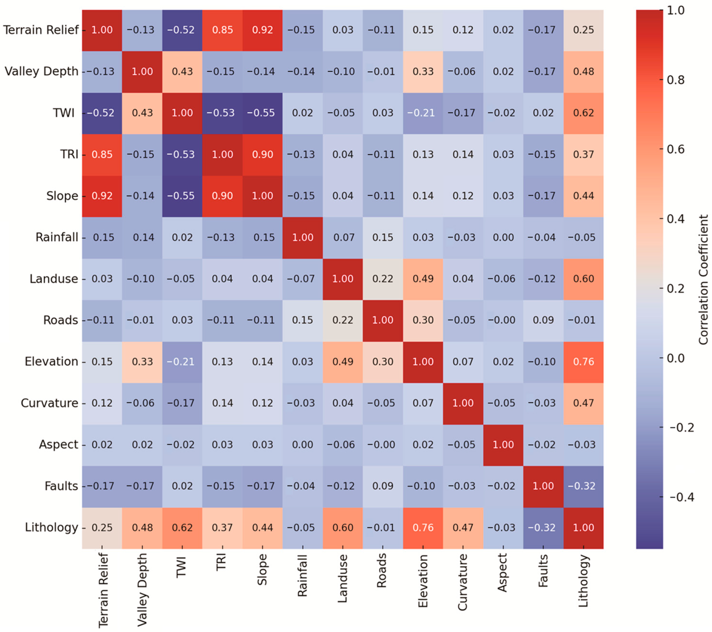
2.3. Statistical Feature Filtering and Assessment
2.4. Machine Learning Techniques
2.5. Validation and Reliability Evaluation
3. Results
3.1. Assessment of Explanatory Variables
3.2. Factors Influencing Landslide Susceptibility
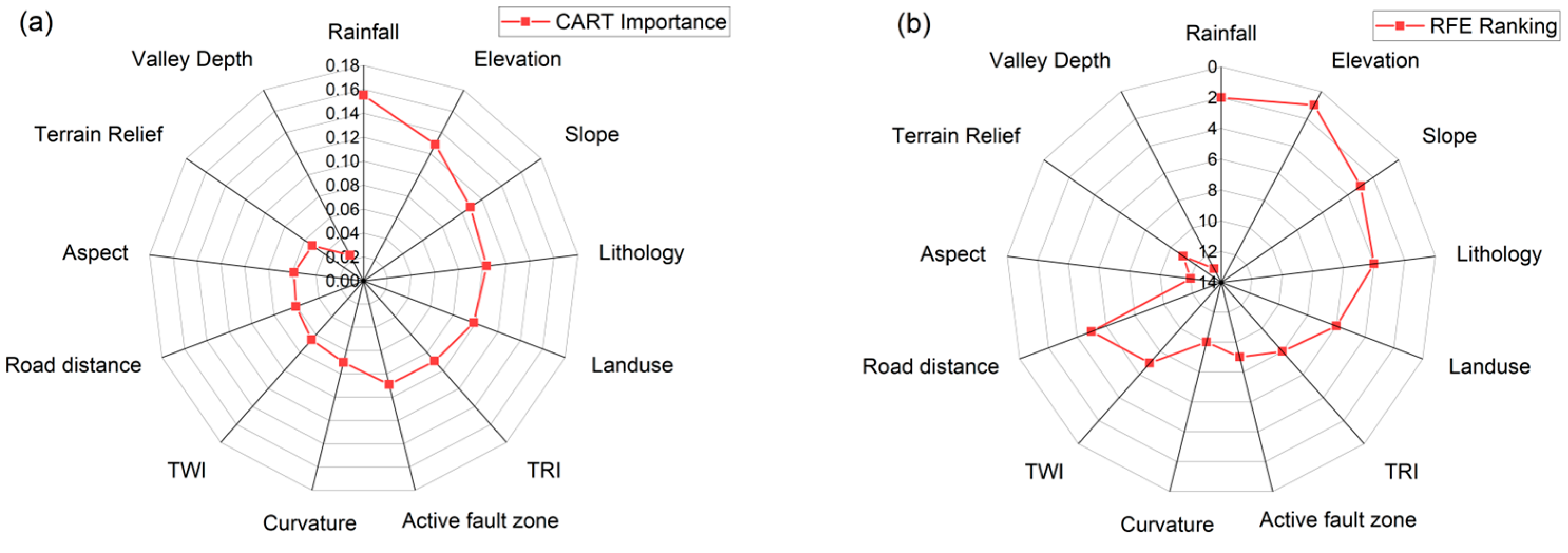
3.3. Feature Priority Selection
3.4. Landslide Susceptibility Analysis
3.5. Models Correlations in LSM
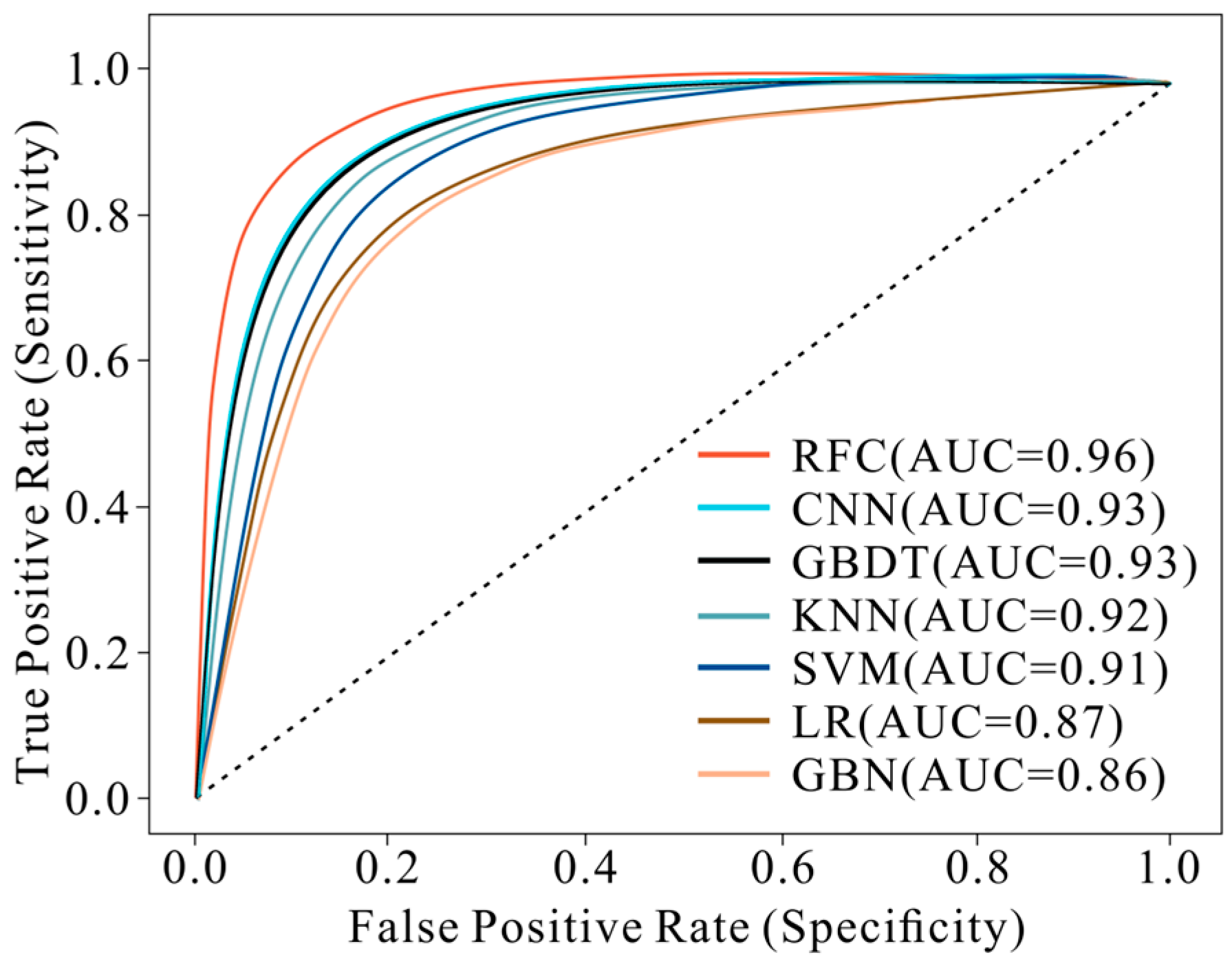
3.6. Models Validation
4. Discussion
5. Conclusions
Author Contributions
Funding
Data Availability Statement
Acknowledgments
Conflicts of Interest
References
- Xie, C.; Huang, Y.; Li, L.; Li, T.; Xu, C. Detailed Inventory and Spatial Distribution Analysis of Rainfall-Induced Landslides in Jiexi County, Guangdong Province, China in August 2018. Sustainability 2023, 15, 13930. [Google Scholar] [CrossRef]
- Chen, W.; Chen, Y.; Tsangaratos, P.; Ilia, I.; Wang, X. Combining Evolutionary Algorithms and Machine Learning Models in Landslide Susceptibility Assessments. Remote Sens. 2020, 12, 3854. [Google Scholar] [CrossRef]
- Ullah, I.; Aslam, B.; Shah, S.H.I.A.; Tariq, A.; Qin, S.; Majeed, M.; Havenith, H.-B. An Integrated Approach of Machine Learning, Remote Sensing, and GIS Data for the Landslide Susceptibility Mapping. Land 2022, 11, 1265. [Google Scholar] [CrossRef]
- Zhuo, L.; Huang, Y.; Zheng, J.; Cao, J.; Guo, D. Landslide Susceptibility Mapping in Guangdong Province, China, Using Random Forest Model and Considering Sample Type and Balance. Sustainability 2023, 15, 9024. [Google Scholar] [CrossRef]
- Islam, F.; Riaz, S.; Ghaffar, B.; Tariq, A.; Shah, S.U.; Nawaz, M.; Hussain, M.L.; Amin, N.U.; Li, Q.; Lu, L.; et al. Landslide Susceptibility Mapping (LSM) of Swat District, Hindu Kush Himalayan Region of Pakistan, Using GIS-Based Bivariate Modeling. Front. Environ. Sci. 2022, 10, 1027423. [Google Scholar] [CrossRef]
- Ali, S.; Biermanns, P.; Haider, R.; Reicherter, K. Landslide Susceptibility Mapping by Using GIS along the China–Pakistan Economic Corridor (Karakoram Highway), Pakistan. Nat. Hazards Earth Syst. Sci. 2018, 19, 999–1022. [Google Scholar] [CrossRef]
- Habumugisha, J.M.; Chen, N.; Rahman, M.; Islam, M.M.; Ahmad, H.; Elbeltagi, A.; Sharma, G.; Liza, S.N.; Dewan, A. Landslide Susceptibility Mapping with Deep Learning Algorithms. Sustainability 2022, 14, 1734. [Google Scholar] [CrossRef]
- Qin, Z.; Zhou, X.; Li, M.; Tong, Y.; Luo, H. Landslide Susceptibility Mapping Based on Resampling Method and FR-CNN: A Case Study of Changdu. Land 2023, 12, 1213. [Google Scholar] [CrossRef]
- Hussain, M.A.; Chen, Z.; Zheng, Y.; Zhou, Y.; Daud, H. Deep Learning and Machine Learning Models for Landslide Susceptibility Mapping with Remote Sensing Data. Remote Sens. 2022, 15, 4703. [Google Scholar] [CrossRef]
- Lucchese, L.V.; De Oliveira, G.G.; Pedrollo, O.C. Investigation of the Influence of Nonoccurrence Sampling on Landslide Susceptibility Assessment Using Artificial Neural Networks. CATENA 2021, 198, 105067. [Google Scholar] [CrossRef]
- Sellers, C. Analysis of Conditioning Factors in Cuenca, Ecuador, for Landslide Susceptibility Maps Generation Employing Machine Learning Methods. Land 2023, 12, 1135. [Google Scholar] [CrossRef]
- Band, L.E.; Moore, I.D. Scale: Landscape Attributes and Geographical Information Systems. Hydrol. Process. 1995, 9, 401–422. [Google Scholar] [CrossRef]
- Sahin, E.K.; Colkesen, I.; Acmali, S.S.; Akgun, A.; Aydinoglu, A.C. Developing Comprehensive Geocomputation Tools for Landslide Susceptibility Mapping: LSM Tool Pack. Comput. Geosci. 2020, 144, 104592. [Google Scholar] [CrossRef]
- Micheletti, N.; Foresti, L.; Robert, S.; Leuenberger, M.; Pedrazzini, A.; Jaboyedoff, M.; Kanevski, M. Machine Learning Feature Selection Methods for Landslide Susceptibility Mapping. Math. Geosci. 2014, 46, 33–57. [Google Scholar] [CrossRef]
- Lee, S.; Hong, S.M.; Jung, H.S. A Support Vector Machine for Landslide Susceptibility Mapping in Gangwon Province, Korea. Sustainability 2017, 9, 48. [Google Scholar] [CrossRef]
- Meena, S.R.; Puliero, S.; Bhuyan, K.; Floris, M.; Catani, F. Assessing the Importance of Conditioning Factor Selection in Landslide Susceptibility for the Province of Belluno. Nat. Hazards Earth Syst. Sci. 2022, 22, 1395–1417. [Google Scholar] [CrossRef]
- Shahzad, N.; Ding, X.; Abbas, S. A Comparative Assessment of Machine Learning Models for Landslide Susceptibility Mapping in the Rugged Terrain of Northern Pakistan. Appl. Sci. 2022, 12, 2280. [Google Scholar] [CrossRef]
- Youssef, A.M.; Pourghasemi, H.R.; Pourtaghi, Z.S.; Al-Katheeri, M.M. Landslide Susceptibility Mapping Using Random Forest, Boosted Regression Tree, Classification and Regression Tree, and General Linear Models. Landslides 2016, 13, 839–856. [Google Scholar] [CrossRef]
- Zhang, H.; Yin, C.; Wang, S.; Guo, B. Landslide Susceptibility Mapping Based on Landslide Classification and Improved Convolutional Neural Networks. Nat. Hazards 2023, 116, 1931–1971. [Google Scholar] [CrossRef]
- Rehman, A.; Song, J.; Haq, F.; Mahmood, S.; Ahamad, M.I.; Basharat, M.; Sajid, M.; Mehmood, M.S. Multi-Hazard Susceptibility Assessment Using the Analytical Hierarchy Process and Frequency Ratio Techniques in the Northwest Himalayas, Pakistan. Remote Sens. 2022, 14, 554. [Google Scholar] [CrossRef]
- Ali, Z.; Qaisar, M.; Mahmood, T.; Shah, M.A.; Iqbal, T.; Serva, L.; Michetti, A.M.; Burton, P.W. The Muzaffarabad, Pakistan, Earthquake of 8 October 2005: Surface Faulting, Environmental Effects and Macroseismic Intensity. Geol. Soc. Lond. Spec. Publ 2009, 316, 155–172. [Google Scholar] [CrossRef]
- Abid, M.; Isleem, H.F.; Shahzada, K.; Khan, A.U.; Kamal Shah, M.; Saeed, S.; Aslam, F. Seismic Hazard Assessment of Shigo Kas Hydro-Power Project (Khyber Pakhtunkhwa, Pakistan). Buildings 2021, 11, 349. [Google Scholar] [CrossRef]
- Dhuime, B.; Bosch, D.; Bodinier, J.; Garrido, C.; Bruguier, O.; Hussain, S.; Dawood, H. Multistage Evolution of the Jijal Ultramafic–Mafic Complex (Kohistan, N Pakistan): Implications for Building the Roots of Island Arcs. Earth Planet. Sci. Lett. 2007, 261, 179–200. [Google Scholar] [CrossRef]
- Khan, M.; Nawaz, S.; Radwan, A.E. New Insights into Tectonic Evolution and Deformation Mechanism of Continental Foreland Fold-Thrust Belt. J. Asian Earth Sci. 2023, 245, 105556. [Google Scholar] [CrossRef]
- Rehman, S.A.; Riaz, Z.; Bui, M.D.; Rutschmann, P. Application of a 1D Numerical Model for Sediment Management in Dasu Hydropower Project. In Proceedings of the 14th International Conference on Environmental Science and Technology, Rhodes, Greece, 3–5 September 2015. [Google Scholar]
- Hastenrath, S.; Greischar, L. The Monsoonal Current Regimes of the Tropical Indian Ocean: Observed Surface Flow Fields and Their Geostrophic and Wind-Driven Components. J. Geophys. Res. Ocean. 1991, 96, 12619–12633. [Google Scholar] [CrossRef]
- Liu, X.; Zhao, C.; Zhang, Q.; Lu, Z.; Li, Z.; Yang, C.; Liu, C. Integration of Sentinel-1 and ALOS/PALSAR-2 SAR Datasets for Mapping Active Landslides along the Jinsha River Corridor, China. Eng. Geol. 2021, 284, 106033. [Google Scholar] [CrossRef]
- Khan, H.; Shafique, M.; Khan, M.A.; Bacha, M.A.; Shah, S.U.; Calligaris, C. Landslide Susceptibility Assessment Using Frequency Ratio, a Case Study of Northern Pakistan. Egypt. J. Remote Sens. Space Sci. 2019, 22, 11–24. [Google Scholar] [CrossRef]
- Fayaz, A.; Latif, M.; Khan, K. Landslide Evaluation and Stabilization between Gilgit ans Thakot along the Karakoram Highway; Geological Survey of Pakistan: Islamabad, Pakistan, 1985. [Google Scholar]
- Khan, K.; Fayaz, A.; Latif, M.; Wazir, A. Rock and Debris Slides between Khunjrab Pass and Gilgit along the Karakoram Highway; Geological Survey of Pakistan: Islamabad, Pakistan, 1986. [Google Scholar]
- Khan, K.; Fayaz, A.; Hussain, M.; Latif, M. Landslides Problems and Their Mitigation along the Karakoram Highway; Geological Survey of Pakistan: Islamabad, Pakistan, 2003. [Google Scholar]
- Hewitt, K. Catastrophic landslides and their effects on the Upper Indus streams, Karakoram Himalaya, northern Pakistan. Geomorphology 1998, 26, 47–80. [Google Scholar] [CrossRef]
- Hussain, M.A.; Chen, Z.; Zheng, Y.; Shoaib, M.; Shah, S.U.; Ali, N.; Afzal, Z. Landslide Susceptibility Mapping Using Machine Learning Algorithm Validated by Persistent Scatterer In-SAR Technique. Sensors 2022, 22, 3119. [Google Scholar] [CrossRef]
- Yao, Z.; Chen, M.; Zhan, J.; Zhuang, J.; Sun, Y.; Yu, Q.; Yu, Z. Refined Landslide Susceptibility Mapping by Integrating the SHAP-CatBoost Model and InSAR Observations: A Case Study of Lishui, Southern China. Appl. Sci. 2023, 13, 12817. [Google Scholar] [CrossRef]
- Ali, N.; Chen, J.; Fu, X.; Ali, R.; Hussain, M.A.; Daud, H.; Hussain, J.; Altalbe, A. Integrating Machine Learning Ensembles for Landslide Susceptibility Mapping in Northern Pakistan. Remote Sens. 2024, 16, 988. [Google Scholar] [CrossRef]
- Sun, X.; Chen, J.; Li, Y.; Rene, N.N. Landslide Susceptibility Mapping along a Rapidly Uplifting River Valley of the Upper Jinsha River, Southeastern Tibetan Plateau, China. Remote Sens. 2022, 14, 1730. [Google Scholar] [CrossRef]
- Yu, H.; Pei, W.; Zhang, J.; Chen, G. Landslide Susceptibility Mapping and Driving Mechanisms in a Vulnerable Region Based on Multiple Machine Learning Models. Remote Sens. 2023, 15, 1886. [Google Scholar] [CrossRef]
- Minh, N.Q.; Huong, N.T.T.; Khanh, P.Q.; Hien, L.P.; Bui, D.T. Impacts of Resampling and Downscaling Digital Elevation Model and Its Morphometric Factors: A Comparison of Hopfield Neural Network, Bilinear, Bicubic, and Kriging Interpolations. Remote Sens. 2024, 16, 819. [Google Scholar] [CrossRef]
- Stojilković, B. Towards Transferable Use of Terrain Ruggedness Component in the Geodiversity Index. Resources 2022, 11, 22. [Google Scholar] [CrossRef]
- Winzeler, H.E.; Owens, P.R.; Read, Q.D.; Libohova, Z.; Ashworth, A.; Sauer, T. Topographic Wetness Index as a Proxy for Soil Moisture in a Hillslope Catena: Flow Algorithms and Map Generalization. Land 2022, 11, 2018. [Google Scholar] [CrossRef]
- Cheng, J.; Dai, X.; Wang, Z.; Li, J.; Qu, G.; Li, W.; She, J.; Wang, Y. Landslide Susceptibility Assessment Model Construction Using Typical Machine Learning for the Three Gorges Reservoir Area in China. Remote Sens. 2022, 14, 2257. [Google Scholar] [CrossRef]
- Shrestha, N. Detecting Multicollinearity in Regression Analysis. Am. J. Appl. Math. Stat. 2020, 8, 39–42. [Google Scholar] [CrossRef]
- Selamat, S.N.; Majid, N.A.; Taha, M.R.; Osman, A. Landslide Susceptibility Model Using Artificial Neural Network (ANN) Approach in Langat River Basin, Selangor, Malaysia. Land 2022, 11, 833. [Google Scholar] [CrossRef]
- Wang, G.; Chen, X.; Chen, W. Spatial Prediction of Landslide Susceptibility Based on GIS and Discriminant Functions. ISPRS Int. J. Geo-Inf. 2020, 9, 144. [Google Scholar] [CrossRef]
- Yin, Y.; Jang-Jaccard, J.; Xu, W.; Singh, A.; Zhu, J.; Sabrina, F.; Kwak, J. IGRF-RFE: A Hybrid Feature Selection Method for MLP-Based Network Intrusion Detection on UNSW-NB15 Dataset. J. Big Data 2023, 10, 15. [Google Scholar] [CrossRef]
- Kavzoglu, T.; Teke, A.; Yilmaz, E.O. Shared Blocks-Based Ensemble Deep Learning for Shallow Landslide Susceptibility Mapping. Remote Sens. 2021, 13, 4776. [Google Scholar] [CrossRef]
- Kamran, K.V.; Feizizadeh, B.; Khorrami, B.; Ebadi, Y. A Comparative Approach of Support Vector Machine Kernel Functions for GIS-Based Landslide Susceptibility Mapping. Appl. Geomat. 2021, 13, 837–851. [Google Scholar] [CrossRef]
- Chen, W.; Pourghasemi, H.R.; Naghibi, S.A. A Comparative Study of Landslide Susceptibility Maps Produced Using Support Vector Machine with Different Kernel Functions and Entropy Data Mining Models in China. Bull. Eng. Geol. Environ. 2018, 77, 647–664. [Google Scholar] [CrossRef]
- Chen, W.; Sun, Z.; Han, J. Landslide Susceptibility Modeling Using Integrated Ensemble Weights of Evidence with Logistic Regression and Random Forest Models. Appl. Sci. 2019, 9, 171. [Google Scholar] [CrossRef]
- Taalab, K.; Cheng, T.; Zhang, Y. Mapping Landslide Susceptibility and Types Using Random Forest. Big Earth Data 2018, 2, 159–178. [Google Scholar] [CrossRef]
- Parmar, A.; Katariya, R.; Patel, V. A Review on Random Forest: An Ensemble Classifier. In Proceedings of the International Conference on Intelligent Data Communication Technologies and Internet of Things (ICICI) 2018, Coimbatore, India, 7–8 August 2018; Springer International Publishing: Cham, Switzerland, 2019; pp. 758–763. [Google Scholar]
- Nikoobakht, S.; Azarafza, M.; Akgün, H.; Derakhshani, R. Landslide Susceptibility Assessment by Using Convolutional Neural Network. Appl. Sci. 2022, 12, 5992. [Google Scholar] [CrossRef]
- Rong, G.; Alu, S.; Li, K.; Su, Y.; Zhang, J.; Zhang, Y.; Li, T. Rainfall Induced Landslide Susceptibility Mapping Based on Bayesian Optimized Random Forest and Gradient Boosting Decision Tree Models—A Case Study of Shuicheng County, China. Water 2020, 12, 3066. [Google Scholar] [CrossRef]
- Song, Y.; Niu, R.; Xu, S.; Ye, R.; Peng, L.; Guo, T.; Chen, T. Landslide Susceptibility Mapping Based on Weighted Gradient Boosting Decision Tree in Wanzhou Section of the Three Gorges Reservoir Area (China). ISPRS Int. J. Geo-Inf. 2018, 8, 4. [Google Scholar] [CrossRef]
- Tang, H.; Wang, C.; An, S.; Wang, Q.; Jiang, C. A Novel Heterogeneous Ensemble Framework Based on Machine Learning Models for Shallow Landslide Susceptibility Mapping. Remote Sens. 2023, 15, 4159. [Google Scholar] [CrossRef]
- Nayak, S.; Bhat, M.; Subba Reddy, N.V.; Ashwath Rao, B. Study of Distance Metrics on K-Nearest Neighbor Algorithm for Star Categorization. J. Phys. Conf. Ser. 2022, 2161, 012004. [Google Scholar] [CrossRef]
- Jati, M.F.K.; Wahyunggoro, O.; Bejo, A.; Adimedha, T.B. Distance Metrics Comparison on K-Nearest Neighbor for Landslide Susceptibility Mapping. In Proceedings of the 2023 IEEE International Conference on Industry 4.0, Artificial Intelligence, and Communications Technology (IAICT), Bali, Indonesia, 13–15 July 2023. [Google Scholar]
- Chen, W.; Zhang, S.; Li, R.; Shahabi, H. Performance Evaluation of the GIS-Based Data Mining Techniques of Best-First Decision Tree, Random Forest, and Naïve Bayes Tree for Landslide Susceptibility Modeling. Sci. Total Environ. 2018, 644, 1006–1018. [Google Scholar] [CrossRef]
- Raia, S.; Alvioli, M.; Rossi, M.; Baum, R.L.; Godt, J.W.; Guzzetti, F. Improving Predictive Power of Physically Based Rainfall-Induced Shallow Landslide Models: A Probabilistic Approach. Geosci. Model. Dev. 2014, 7, 495–514. [Google Scholar] [CrossRef]
- Vakhshoori, V.; Zare, M. Is the ROC Curve a Reliable Tool to Compare the Validity of Landslide Susceptibility Maps? Geomat. Nat. Hazards Risk 2018, 9, 249–266. [Google Scholar] [CrossRef]
- Lei, T.; Zhang, Y.; Lv, Z.; Li, S.; Liu, S.; Nandi, A.K. Landslide Inventory Mapping from Bitemporal Images Using Deep Convolutional Neural Networks. IEEE Geosci. Remote Sens. Lett. 2019, 16, 982–986. [Google Scholar] [CrossRef]
- Adugna, T.; Xu, W.; Fan, J. Comparison of Random Forest and Support Vector Machine Classifiers for Regional Land Cover Mapping Using Coarse Resolution FY-3C Images. Remote Sens. 2022, 14, 574. [Google Scholar] [CrossRef]
- Datta, A.; Luirei, K.; Mehta, M. Slope Instabilities and Evolution of Tectonic Geomorphology Along the Strike of the Main Boundary Thrust Zone in the Western Himalaya, India. Nat. Hazards Res. 2023, 4, 118–133. [Google Scholar] [CrossRef]
- Qiu, H.; Su, L.; Tang, B.; Yang, D.; Ullah, M.; Zhu, Y.; Kamp, U. The Effect of Location and Geometric Properties of Landslides Caused by Rainstorms and Earthquakes. Earth Surf. Process. Landf. 2024, 49, 2067–2079. [Google Scholar] [CrossRef]
- Qiu, H.; Zhu, Y.; Zhou, W.; Sun, H.; He, J.; Liu, Z. Influence of DEM Resolution on Landslide Simulation Performance Based on the Scoops3D Model. Geomat. Nat. Hazards Risk 2022, 13, 1663–1681. [Google Scholar] [CrossRef]
- Shao, X.; Xu, C.; Ma, S. Preliminary Analysis of Coseismic Landslides Induced by the 1 June 2022 Ms 6.1 Lushan Earthquake, China. Sustainability 2022, 14, 16554. [Google Scholar] [CrossRef]
- Ye, B.; Qiu, H.; Tang, B.; Liu, Y.; Liu, Z.; Jiang, X.; Yang, D.; Ullah, M.; Zhu, Y.; Kamp, U. Creep Deformation Monitoring of Landslides in a Reservoir Area. J. Hydrol. 2024, 632, 130905. [Google Scholar] [CrossRef]
- Pandita, S.; Kumar, V.; Dutt, H.C. Environmental Variables Vis-à-Vis Distribution of Herbaceous Tracheophytes on Northern Sub-Slopes in Western Himalayan Ecotone. Ecol. Process 2019, 8, 45. [Google Scholar] [CrossRef]
- Yang, D.; Qiu, H.; Ye, B.; Liu, Y.; Zhang, J.; Zhu, Y. Distribution and Recurrence of Warming-induced Retrogressive Thaw Slumps on the Central Qinghai-Tibet Plateau. J. Geophys. Res. Earth Surf. 2023, 128, e2022JF007047. [Google Scholar] [CrossRef]
- Liu, Y.; Qiu, H.; Kamp, U.; Wang, N.; Wang, J.; Huang, C.; Tang, B. Higher Temperature Sensitivity of Retrogressive Thaw Slump Activity in the Arctic Compared to the Third Pole. Sci. Total Environ. 2024, 914, 170007. [Google Scholar] [CrossRef] [PubMed]
- Saleem, N.; Huq, M.E.; Twumasi, N.Y.D.; Javed, A.; Sajjad, A. Parameters Derived from and/or Used with Digital Elevation Models (DEMs) for Landslide Susceptibility Mapping and Landslide Risk Assessment: A Review. ISPRS Int. J. Geo-Inf. 2019, 8, 545. [Google Scholar] [CrossRef]
- Pes, B. Learning from High-Dimensional and Class-Imbalanced Datasets Using Random Forests. Information 2021, 12, 286. [Google Scholar] [CrossRef]
- Can, R.; Kocaman, S.; Gokceoglu, C. A Comprehensive Assessment of XGBoost Algorithm for Landslide Susceptibility Mapping in the Upper Basin of Ataturk Dam, Turkey. Appl. Sci. 2021, 11, 4993. [Google Scholar] [CrossRef]
- Luyao, W.; Haijun, Q.; Wenqi, Z.; Yaru, Z.; Zijing, L.; Shuyue, M.; Dongdong, Y.; Bingzhe, T. The post-failure spatiotemporal deformation of certain translational landslides may follow the pre-failure pattern. Remote Sens. 2022, 14, 2333. [Google Scholar] [CrossRef]
- Dai, X.; Zhu, Y.; Sun, K.; Zou, Q.; Zhao, S.; Li, W.; Hu, L.; Wang, S. Examining the Spatially Varying Relationships between Landslide Susceptibility and Conditioning Factors Using a Geographical Random Forest Approach: A Case Study in Liangshan, China. Remote Sens. 2023, 15, 1513. [Google Scholar] [CrossRef]
- Zhou, W.; Qiu, H.; Wang, L.; Pei, Y.; Tang, B.; Ma, S.; Yang, D.; Cao, M. Combining rainfall-induced shallow landslides and subsequent debris flows for hazard chain prediction. Catena 2022, 213, 106199. [Google Scholar] [CrossRef]
- Shah, N.A.; Shafique, M.; Ishfaq, M.; Faisal, K.; Van der Meijde, M. Integrated Approach for Landslide Risk Assessment Using Geoinformation Tools and Field Data in Hindukush Mountain Ranges, Northern Pakistan. Sustainability 2023, 15, 3102. [Google Scholar] [CrossRef]
- Liu, Z.; Qiu, H.; Zhu, Y.; Liu, Y.; Yang, D.; Ma, S.; Zhang, J.; Wang, Y.; Wang, L.; Tang, B. Efficient Identification and Monitoring of Landslides by Time-Series InSAR Combining Single- and Multi-Look Phases. Remote Sens. 2022, 14, 1026. [Google Scholar] [CrossRef]
- Alem, G. Urban Plans and Conflicting Interests in Sustainable Cross-Boundary Land Governance, the Case of National Urban and Regional Plans in Ethiopia. Sustainability 2021, 13, 3081. [Google Scholar] [CrossRef]
- Zhu, Y.; Qiu, H.; Yang, D.; Liu, Z.; Ma, S.; Pei, Y.; He, J.; Du, C.; Sun, H. Pre- and post-failure spatiotemporal evolution of loess landslides: A case study of the Jiangou landslide in Ledu, China. Landslides 2021, 18, 3475–3484. [Google Scholar] [CrossRef]


| Sl. No. | Conditioning Factors | Source | Spatial Resolution |
|---|---|---|---|
| 1 | Slope | SRTM 30 m DEM | 30 mt. |
| 2 | Aspect | SRTM 30 m DEM | 30 mt. |
| 3 | Curvature | SRTM 30 m DEM | 30 mt. |
| 4 | Land use land cover | USGS Global Land Cover (https://www.usgs.gov/centers/eros/science/usgs-eros-archive-landsat-global-land-cover) (accessed on 2 February 2024) | 30 mt. (resampled) |
| 5 | Lithology | National Library of Australia (http://nla.gov.au/nla.obj-233602228) (accessed on 2 February 2024) | 30 mt. (resampled) |
| 6 | Distance from fault | National Library of Australia (http://nla.gov.au/nla.obj-233602228) (accessed on 2 February 2024) | 30 mt. (resampled) |
| 7 | Distance from the road | Natural Earth Data (https://www.naturalearthdata.com/downloads/10m-cultural-vectors/) (accessed on 2 February 2024) | 30 mt. (resampled) |
| 8 | Terrain Relief | SRTM 30 m DEM | 30 mt. |
| 9 | Valley Depth | SRTM 30 m DEM | 30 mt. |
| 10 | Topographic Wetness Index (TWI) | SRTM 30 m DEM | 30 mt. |
| 11 | Terrain Ruggedness Index (TRI) | SRTM 30 m DEM | 30 mt. |
| 12 | Elevation | SRTM 30 m DEM | 30 mt. |
| 13 | Rainfall | Climate Hazards Group InfraRed Precipitation with Station data | 30 mt. (rescaled) |
| Variable | VIF | TOL |
|---|---|---|
| Distance to active faults | 1.10 | 0.96 |
| Valley Depth | 1.18 | 0.85 |
| TWI | 1.36 | 0.73 |
| Distance to Roads | 1.55 | 0.65 |
| Curvature | 1.73 | 0.58 |
| Aspect | 1.91 | 0.52 |
| Terrain Relief | 2.09 | 0.48 |
| Land Use | 2.27 | 0.44 |
| Slope | 2.46 | 0.41 |
| TRI | 2.64 | 0.38 |
| Lithology | 2.74 | 0.36 |
| Rainfall | 2.82 | 0.36 |
| Elevation | 2.98 | 0.33 |
| SVM | |||
| Susceptibility | Pixel Amount | Area (%) | Landslide Frequency (%) |
| Very Low | 62,554,112 | 26.68 | 1.93 |
| Low | 97,580,722 | 41.62 | 6.9 |
| Moderate | 28,868,401 | 12.31 | 7.55 |
| High | 14,575,374 | 6.22 | 10.81 |
| Very High | 30,893,955 | 13.18 | 72.8 |
| RFC | |||
| Susceptibility | Pixel Amount | Area (%) | Landslide Frequency (%) |
| Very Low | 139,775,856 | 59.61 | 3.5 |
| Low | 43,713,122 | 18.64 | 3.73 |
| Moderate | 21,461,542 | 9.15 | 4.42 |
| High | 15,208,584 | 6.49 | 13.02 |
| Very High | 14,313,460 | 6.1 | 75.33 |
| LR | |||
| Susceptibility | Pixel Amount | Area (%) | Landslide Frequency (%) |
| Very Low | 93,261,404 | 39.77 | 6.63 |
| Low | 57,940,244 | 24.71 | 7.32 |
| Moderate | 37,267,200 | 15.89 | 11.5 |
| High | 25,901,038 | 11.05 | 20.98 |
| Very High | 20,102,678 | 8.57 | 53.57 |
| KNN | |||
| Susceptibility | Pixel Amount | Area (%) | Landslide Frequency (%) |
| Very Low | 139,571,787 | 59.53 | 4.28 |
| Low | 32,999,116 | 14.07 | 5.43 |
| Moderate | 20,573,972 | 8.77 | 7.55 |
| High | 15,290,956 | 6.52 | 11.04 |
| Very High | 26,036,733 | 11.1 | 71.7 |
| GBN | |||
| Susceptibility | Pixel Amount | Area (%) | Landslide Frequency (%) |
| Very Low | 138,211,363 | 58.95 | 6.76 |
| Low | 29,733,311 | 12.68 | 7.46 |
| Moderate | 17,832,691 | 7.61 | 11.87 |
| High | 16,821,114 | 7.17 | 12.43 |
| Very High | 31,874,085 | 13.59 | 61.48 |
| GBDT | |||
| Susceptibility | Pixel Amount | Area (%) | Landslide Frequency (%) |
| Very Low | 110,612,605 | 47.18 | 3.73 |
| Low | 55,933,064 | 23.85 | 5.66 |
| Moderate | 28,009,937 | 11.95 | 9.76 |
| High | 17,227,718 | 7.35 | 16.94 |
| Very High | 22,689,240 | 9.68 | 63.92 |
| CNN | |||
| Susceptibility | Pixel Amount | Area (%) | Landslide Frequency (%) |
| Very Low | 136,521,785 | 58.23 | 0.8% |
| Low | 41,280,794 | 17.61 | 2.9% |
| Moderate | 21,444,077 | 9.15 | 8.2% |
| High | 16,783,057 | 7.16 | 18.2% |
| Very High | 18,442,851 | 7.87 | 67.4% |
| Model Pair | p-Value | Significance | Correlation |
|---|---|---|---|
| SVM vs. RFC | 0.25 | high | Moderate |
| SVM vs. LR | 0.875 | high | Strong |
| SVM vs. KNN | 0.25 | high | Moderate |
| SVM vs. GBN | 0.875 | high | Strong |
| SVM vs. GBDT | 0.875 | high | Strong |
| SVM vs. CNN | 0.25 | high | Moderate |
| RFC vs. LR | 0.125 | high | Weak |
| RFC vs. KNN | 0.125 | high | Weak |
| RFC vs. GBN | 0.125 | high | Weak |
| RFC vs. GBDT | 0.125 | high | Weak |
| RFC vs. CNN | 0.125 | high | Weak |
| LR vs. KNN | 0.125 | high | Weak |
| LR vs. GBN | 0.625 | high | Moderate |
| LR vs. GBDT | 0.625 | high | Moderate |
| LR vs. CNN | 0.125 | high | Weak |
| KNN vs. GBN | 0.125 | high | Weak |
| KNN vs. GBDT | 0.125 | high | Weak |
| KNN vs. CNN | 0.125 | high | Weak |
| GBN vs. GBDT | 0.875 | high | Strong |
| GBN vs. CNN | 0.125 | high | Weak |
| GBDT vs. CNN | 0.125 | high | Weak |
| Model | AUC | F-Score |
|---|---|---|
| SVM | 0.91 | 0.69 |
| CNN | 0.93 | 0.84 |
| RFC | 0.96 | 0.86 |
| LR | 0.87 | 0.57 |
| KNN | 0.92 | 0.74 |
| GBN | 0.86 | 0.63 |
| GBDT | 0.93 | 0.61 |
Disclaimer/Publisher’s Note: The statements, opinions and data contained in all publications are solely those of the individual author(s) and contributor(s) and not of MDPI and/or the editor(s). MDPI and/or the editor(s) disclaim responsibility for any injury to people or property resulting from any ideas, methods, instructions or products referred to in the content. |
© 2024 by the authors. Licensee MDPI, Basel, Switzerland. This article is an open access article distributed under the terms and conditions of the Creative Commons Attribution (CC BY) license (https://creativecommons.org/licenses/by/4.0/).
Share and Cite
Ullah, M.; Tang, B.; Huangfu, W.; Yang, D.; Wei, Y.; Qiu, H. Machine Learning-Driven Landslide Susceptibility Mapping in the Himalayan China–Pakistan Economic Corridor Region. Land 2024, 13, 1011. https://doi.org/10.3390/land13071011
Ullah M, Tang B, Huangfu W, Yang D, Wei Y, Qiu H. Machine Learning-Driven Landslide Susceptibility Mapping in the Himalayan China–Pakistan Economic Corridor Region. Land. 2024; 13(7):1011. https://doi.org/10.3390/land13071011
Chicago/Turabian StyleUllah, Mohib, Bingzhe Tang, Wenchao Huangfu, Dongdong Yang, Yingdong Wei, and Haijun Qiu. 2024. "Machine Learning-Driven Landslide Susceptibility Mapping in the Himalayan China–Pakistan Economic Corridor Region" Land 13, no. 7: 1011. https://doi.org/10.3390/land13071011
APA StyleUllah, M., Tang, B., Huangfu, W., Yang, D., Wei, Y., & Qiu, H. (2024). Machine Learning-Driven Landslide Susceptibility Mapping in the Himalayan China–Pakistan Economic Corridor Region. Land, 13(7), 1011. https://doi.org/10.3390/land13071011