Optimizing Urban Green Spaces for Air Quality Improvement: A Multiscale Land Use/Land Cover Synergy Practical Framework in Wuhan, China

Abstract

Air pollution, particularly fine particulate matter (PM_2.5), poses a significant health risk, especially in high-density urban areas. Urban green space (UGS) can effectively mitigate this pollution. Despite their potential, strategies for effectively leveraging Land Use/Land Cover (LULC) optimization to combat PM_2.5 remain largely unexplored. Ordinary least squares (OLS), geographically weighted regression (GWR) and multiscale geographically weighted regression (MGWR) were employed to investigate the spatial heterogeneity relationship between UGS conversion and PM_2.5 fluctuations across various scales and evolutionary stages, developing a multiscale practical framework for LULC synergy in combating air pollution. The areas of UGSs to/from other LULCs, PM_2.5 concentrations and corresponding variation zones exhibited significant spatial clustering. These UGS conversions explained more than 65% of the PM_2.5 changes in the study area, peaking at 76.4% explanatory power in the fourth stage. Compared to global spatial analysis (OLS: 0–0.48), local spatial regression analysis significantly improved the R² value (GWR: 0.32–0.75, MGWR: 0.48–0.90), but the fitting quality of local spatial regression analysis decreased with increasing scale, highlighting the importance of scale diagnosis. A 2 km scale was identified as optimal for assessing the spatial heterogeneity impact of UGS and other LULC conversions on PM_2.5 changes. Conversion areas from water bodies and bare land to UGSs maintain stable local spatial properties at this scale (bandwidths: 44–99). Our research provides new insights into LULC management and planning, offering a coordinated approach to mitigating urban air pollution. Additionally, a practical framework was established for addressing spatially continuous variables such as PM_2.5, revealing effective approaches for addressing urban environmental issues.

1. Introduction

By 2050, 70% of the global population is projected to reside in urban areas [1]. Air pollution, particularly particulate matter (PM_2.5), has been identified as a significant public health threat and is responsible for an estimated 7 million premature deaths annually [2]. PM_2.5 not only has direct impacts on public health, notably causing respiratory diseases [3,4], but also exacerbates other health risks [5]. For example, studies have demonstrated that the combination of PM_2.5 and COVID-19 significantly increases the risk of severe outcomes and fatalities [6,7,8]. In China, many cities have reported PM_2.5 concentrations exceeding WHO standards, which were lowered from 10 μg/m³ to 5 μg/m³ in September 2021. Adhering to this revised standard could reduce global fatalities related to PM_2.5 by approximately 80% [2]. Therefore, controlling PM_2.5 pollution is imperative for human health and has emerged as a priority for addressing global environmental concerns.

Effectively reducing PM_2.5 concentrations is crucial in addressing public health issues arising from air pollution. PM_2.5 levels are significantly influenced by land use and land cover (LULC) changes, with urban green space (UGS) serving as a pivotal LULC type for significantly mitigating PM_2.5 through enhanced adsorption [9], microclimate regulation [10], improved ventilation [11], and optimized plant configurations [12]. Previous studies have focused predominantly on the relationship between PM_2.5 concentrations and UGSs based on vegetation type (e.g., grassland or forest), quantitative indicators (e.g., area, NDVI, and green coverage), quality indicators (e.g., connectivity), and morphological indicators (e.g., aggregation and irregularity) [12,13,14]. While these studies have enhanced our understanding of the relationship between UGSs as a single LULC type and PM_2.5 levels, their application in practical urban planning is still limited. Given the dynamic changes in LULCs during urbanization [15,16], particularly the long-term quantitative and spatial variations among LULCs, it is crucial to explore the links between UGSs and environmental crises such as PM_2.5 and carbon emissions from the perspective of urban LULC transformations. This approach is more aligned with real-world planning scenarios [17]. Recently, the link between LULC transformations and urban environmental issues, such as heat and PM_2.5, has garnered increasing attention [9,18,19]. However, these studies tend to focus on interannual variable relationships, often overlooking the exploration of underlying connections in these variable changes. Moreover, the availability of high-precision, spatiotemporally continuous PM_2.5 data provided by machine learning technologies [20] offers key data support for long-term systematic studies on the impact of UGS and other LULC evolution on PM_2.5.

In addition, scale is a fundamental concept in geographical research, with scale diagnosis being a critical prerequisite for assessing the feasibility of optimization measures [21]. Studies indicate that the impact of UGSs on PM_2.5 exhibits scale effects, encompassing physical spatial scales (e.g., administrative districts/areas) and suitable scales for analysis methods (e.g., global and local spatial regression analysis). Research confined to specific administrative boundaries (e.g., cities or provinces) may overlook these scale effects in relationships [22,23,24,25]. For instance, Cai et al., (2020) reported that the influence of grasslands on PM_2.5 was underestimated in small-scale studies [13], while Li et al., (2021) observed varied impacts of landscape indices on PM_2.5 across urban and neighborhood scales [26]. Methods for defining study scopes based on LULC types and employing grid-based geographical scaling, in contrast to administrative scales, offer greater flexibility, accounting for spatial spillover effects of PM_2.5 pollution and focusing on more microscales, thereby laying a foundation for developing UGS optimization strategies [21]. In exploring methods for researching the UGS-PM_2.5 relationship, existing studies have predominantly employed global regression methods such as simple correlation analysis or ordinary least squares linear regression (OLS) [9]. Geographically weighted regression (GWR), a local regression analysis method, more effectively addresses local spatial relationships [27]; however, its reliance on the assumption of uniform local effects for all explanatory variables may lead to inaccurate conclusions [21,28]. The latest multiscale geographically weighted regression (MGWR) model releases this assumption and is considered a significant innovation in spatial analysis [28,29,30]. However, current research on collaborative LULC optimization to address environmental issues is relatively rare, and few studies have investigated whether OLS, GWR, and MGWR have appropriate analysis scales.

In major urban built-up areas, LULC changes are particularly intense. The expansion of construction land notably encroaches upon UGSs, leading to significant UGS loss [22]. Overall, exploring UGS evolution through different LULC transformations aids in understanding the driving factors of UGSs and lays the foundation for optimization. Analyzing the impacts of UGSs and other LULC transformations on PM_2.5 concentrations offers theoretical support for the collaborative optimization of UGSs and other LULCs to reduce PM_2.5 concentrations. Wuhan was chosen as the research area for several reasons. First, its extensive research history provides well-documented LULC changes over the past 20 years, enabling a comprehensive analysis of UGS and other LULC transformations [31,32,33]. Second, as a megacity with a high population density, Wuhan experiences severe PM_2.5 pollution, making it an ideal case study for understanding the impacts of urbanization on air quality [34,35,36]. Additionally, Wuhan’s diverse landscape, especially water, along with rapid urban expansion offer an opportunity to study the spatial dynamics of LULC and its environmental consequences.

This study examined the spatiotemporal evolution of UGSs and other LULCs, revealing their profound interconnections with fluctuations in PM_2.5 concentrations. The analysis is based on five periods of Landsat remote sensing images (2000, 2005, 2010, 2015, and 2020) at four geographic grid scales (1 km, 2 km, 3 km, and 5 km). Global and local spatial regression analysis are employed to answer several questions (Figure 1).

Finally, this paper introduces a comprehensive multiscale practice framework to mitigate PM_2.5 pollution and concurrently provides a methodological approach for elucidating interconnections between the urban heat island effect, carbon emissions, and UGSs, from a pragmatic perspective.

2. Methodology

2.1. Study Area and Data Processing

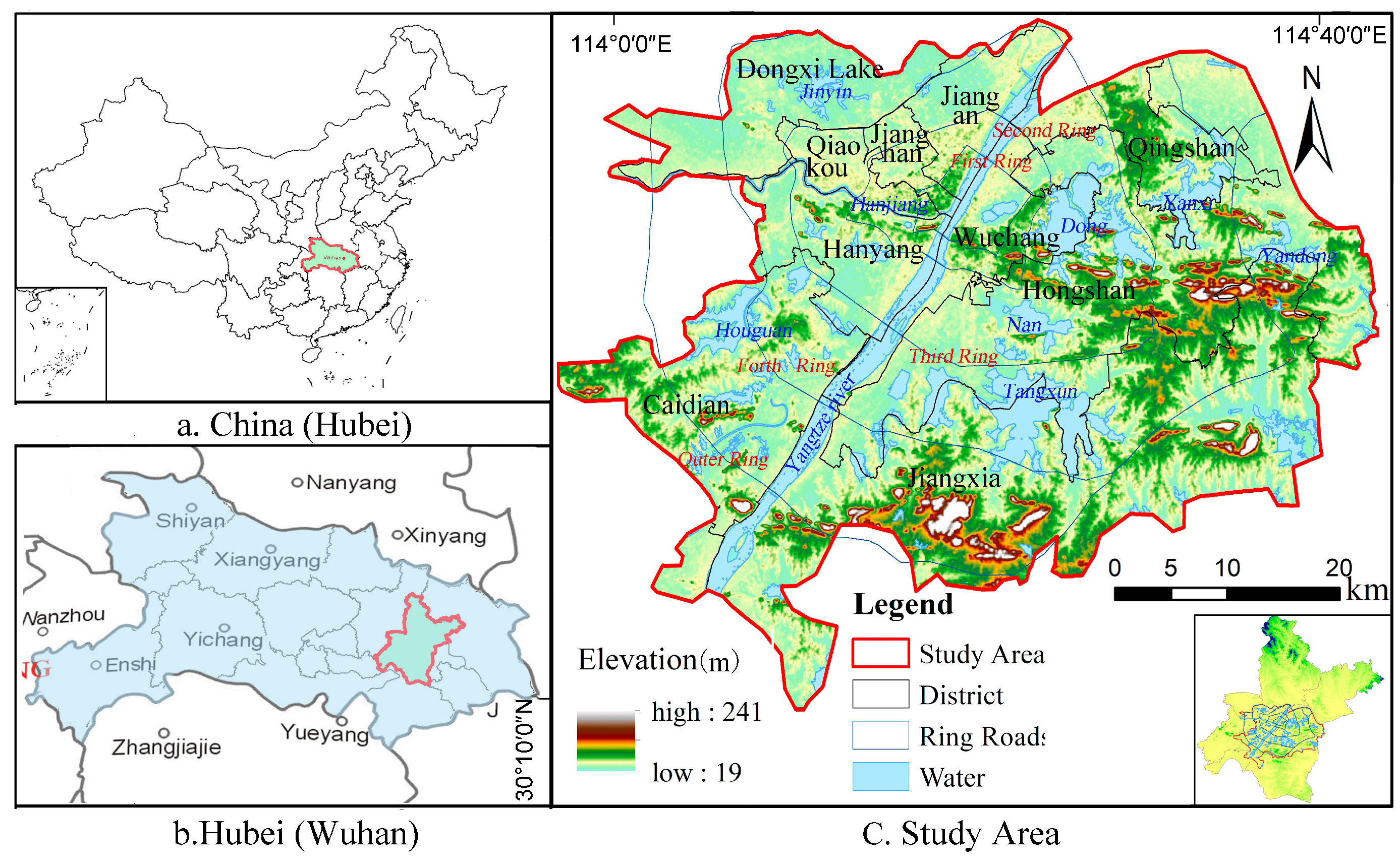
2.1.1. Study Area

Situated in central China, Wuhan (113°41′ E to 115°05′ E, 29°58′ N to 31°22′ N) spans 8569 km² and, as of 2022, hosts a permanent population of 13.74 million people with an urbanization rate of 84.7%. This pivotal megacity has experienced a subtropical monsoonal humid climate, as evidenced by an average annual rainfall of 1100 mm and a temperature range of 15.8 to 17.5 °C over the last three decades [37]. Notably, Wuhan is affected by severe PM_2.5 pollution, a major health concern in densely populated urban areas of China [38]. The city, bisected by the Yangtze River, comprises 13 districts, including Wuchang, Hankou, and Hanyang. The study encompasses seven central urban districts—Jianghan, Jiang’an, Qiaokou, Wuchang, Hongshan, Qingshan, and Hanyang—and two districts witnessing significant urban expansion—Caidian and Jiangxia—collectively covering approximately 1924 km² (Figure 2).

2.1.2. Data Source and Processing

(1) LULC in the study area

Multispectral LULC data covering five distinct periods (2000, 2005, 2010, 2015, and 2020) and vegetation peak data from May to October were obtained from the Geospatial Data Cloud (http://www.gscloud.cn/search) (accessed on 3 July 2021), featuring a cloud-free resolution of 30 m (Table S1, Figure S1a). The image resolution was enhanced to 15 m (Figure S1b) using Gram-Schmidt Pan Sharpening [39] and nearest neighbor resampling [40], thereby improving the LULC classification accuracy. In this process, band fusions (5th, 4th, 3rd and 6th, 5th, and 4th) were employed for UGS classification (Figure S1c). Employing Envi5.4, LULCs were classified as UGS, construction land, water, or bare land [32,41], with a separability index higher than 1.9 [42] (Figure S1d). The classification accuracy, verified through a confusion matrix (detailed in Section 2.3), exceeded 90%, meeting the precision targets. Finally, modal filtering, boundary cleaning, and Nibble processing in ArcMap 10.7 (Figure S1f) were utilized to produce spatial LULC maps for each period (Figure 3a–e), along with their area and percentage data (Figure 3f).

(2) PM_2.5 data and geographic grids

The original annual average PM_2.5 data at five years (2000, 2005, 2010, 2015, and 2020) in the study area were derived from moderate-resolution imaging spectroradiometer (MODIS), as provided by Wei et al., (2020; 2021) [43,44]. These data were calculated using the Space-Time Extra-Trees (STET) model at a resolution of 1 km, achieving high cross-validation accuracy (CV-R² = 0.86–0.90) and predictive R² values (0.80–0.82), surpassing previous studies (https://weijing-rs.github.io/product.html) (accessed on 3 July 2021). The PM_2.5 data have been widely applied in the public health [45,46], environmental [47], and economic sectors [48]. However, in some locations within our study area, there were gaps in the original PM_2.5 data due to factors such as cloud cover (Figure 4a). To address these gaps, we implemented the following steps: first, 10,000 and 5000 free points were set within the original dataset using ArcMap 10.8, excluding locations without data. Using the “Extract Values to Points” tool, the PM_2.5 values at these points were extracted. These values were then used to generate two complete PM_2.5 datasets for the study area based on kriging interpolation [49]. Second, we used an additional 5000 free points to extract three sets of 5000 PM_2.5 values from the predicted complete datasets and the original data. Third, we conducted Pearson correlation tests between these sets to validate the accuracy of the supplemented data. The results showed that the supplemented PM_2.5 data obtained using 5000 predictive points maintained a higher level of accuracy compared to the results predicted with 10,000 points (R² = 0.977) (Figure 4h). Ultimately, PM_2.5 concentration data for the five periods were obtained using 5000 predictive points following the steps outlined above (Figure 4b–f), and Figure 4g shows PM_2.5 concentrations for the 5 years. Additionally, to examine the scale effects of UGSs and other LULC transformations on PM_2.5, the study area was divided into different-size grids (1 km × 1 km, 2 km × 2 km, 3 km × 3 km, and 5 km × 5 km) created with the Fishnet tool in ArcMap 10.7, yielding 1741, 430, 189, and 69 effective research units (Figure S2).

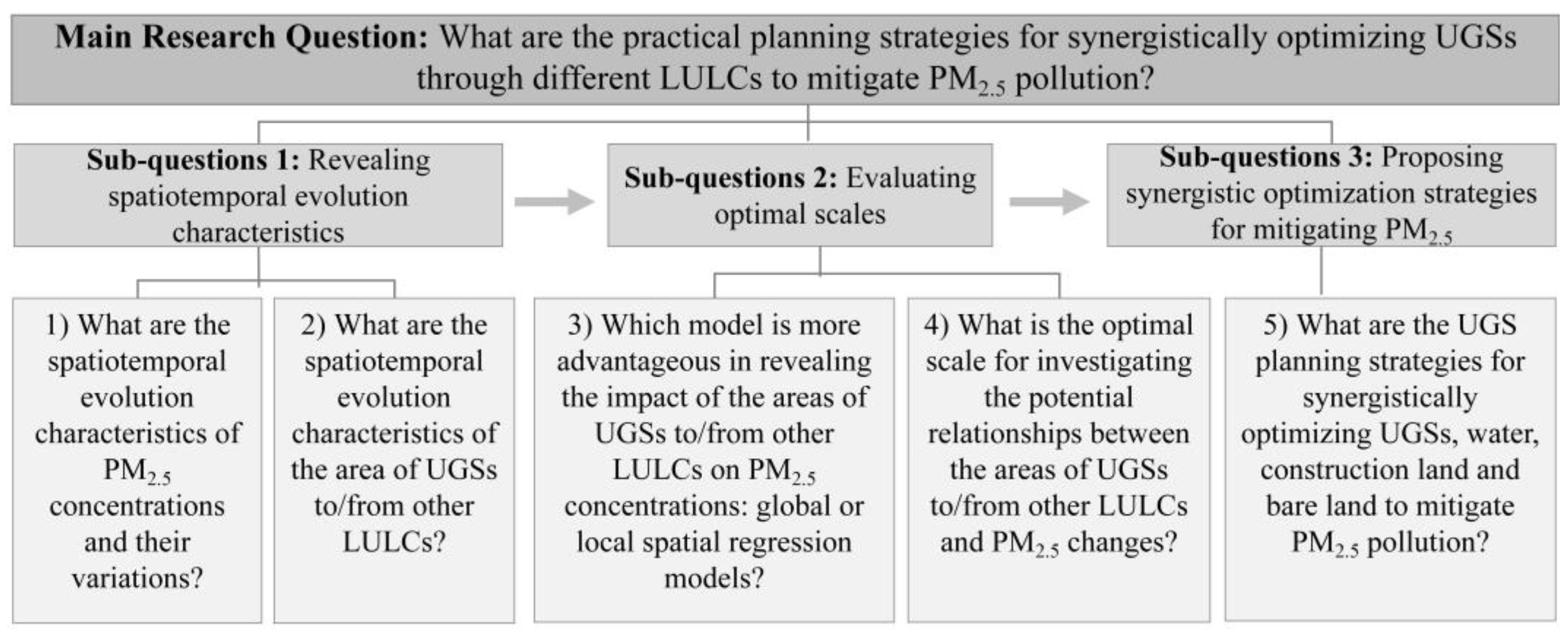
2.2. Research Framework

This research computed the spatial transitions of UGSs to/from the other three LULC categories, as well as the respective annual mean PM_2.5 concentration variations, across four intervals from 2000 to 2020. Compared to other LULCs, UGSs can directly absorb PM_2.5 through vegetation and indirectly mitigate PM_2.5 pollution by improving ventilation and microclimates through changes in vegetation type [50], quantity, spatial layout, and structure (Section 1). Therefore, UGSs are important LULC types for mitigating PM_2.5 pollution. In contrast, other LULCs, such as construction land, are significant sources of PM_2.5 emissions due to high human activity intensity [51]. Thus, analyzing the potential impact mechanisms of the quantity and spatial changes of UGSs to/from other LULCs on PM_2.5 changes from a dynamic perspective is more aligned with the realities of urban construction than analyzing the impact of UGSs on PM_2.5 alone. The specific steps of this research are as follows: first, the LULC conversion into UGS within the study area was assessed using the concept of LULC conversion efficiency (Equation (3)). This was followed by a spatial autocorrelation analysis that quantified the spatial dependency between the UGS conversion locations and PM_2.5 concentration changes, laying the foundation for further spatial regression analysis. Subsequently, the scale effects of UGS on PM_2.5 reduction demonstrated by previous studies were considered. For instance, Wan et al., (2020) found that UGSs with a width of 15–25 m exert the most significant effect on reducing PM_2.5 [50]. Wu et al., (2018) also found that at scales smaller than 2 km, the edge length of UGSs exerts a more pronounced effect on PM_2.5 reduction than their area [52]. Therefore, determining a reasonable analysis scale is crucial. In this study, spatial regression analysis was conducted across four geographic scales to determine the scale effects on the relationship between UGS conversion and PM_2.5 concentration changes, both globally and locally, to identify the optimal analysis scale. Subsequently, at this scale, local R² values and local regression coefficients (LRCs) relating to UGS conversion spaces and PM_2.5 concentration changes were derived via MGWR, with higher absolute values of LRCs (|LRC|) indicating a stronger relationship between the two. This led to the proposal of a collaborative optimization strategy for air pollution mitigation in LULCs (Figure 5).

2.3. Confusion Matrix and LULC Evolution

The confusion matrix is a method for accuracy assessment that encompasses metrics such as producer accuracy (PA), user accuracy (UA), and the kappa coefficient (K). K is used to calculate the degree of overlap between two images, with values ranging from 0 (no overlap) to 1 (perfect overlap). In this study, Equation (1) was used to ascertain the extent of LULC changes within the designated area [41]. Additionally, the efficiency of LULC conversion is quantified as the percentage of one LULC that transforms into another over a specified period, calculated using Equation (3).

$$K=\left(\frac{{\displaystyle {\sum }_{i=1}^r{x}_{ii}}}{N}-\frac{{\displaystyle {\sum }_{i=1}^r\left(x_i+x_{i+}\right)}}{N^2}\right)/\left(1-\frac{{\displaystyle {\sum }_{i=1}^r\left(x_i+x_{i+}\right)}}{N^2}\right)$$

(1)

$$D=\left(1-K\right)\times \raisebox{1ex}{$1$}\!\left/ \!\raisebox{-1ex}{$T$}\right.\times 100\%$$

(2)

$$R_{ij}=\frac{A_{ij}(a)}{|A_i(b)-A_i(a)|}\times \frac{1}{T}\times 100\% (\mathit{i}(\mathit{j})=1,2\dots ,n,\mathrm{representing\; the\; type\; of\; LULC})$$

(3)

where r represents the number of rows in the LULC matrix for the study year, x_ii is the number of combination types along the diagonal, x_i+ is the total observations in row i, x_+i is the total observations in column i, and N is the total number of grids. T represents the interval years of LULC, and D represents the fluctuation degree of LULC types. R_ij denotes the conversion rate of LULC type i to type j, and A_i(a) and A_i(b) represent the areas of type i in years a and b, respectively.

2.4. Annual Concentration and Difference Calculation for PM_2.5

Unlike simple averaging, the weighted average was used to calculate the proportional area of different data in space [34], thus revealing significant spatial attributes. This method is used to calculate the PM_2.5 concentration for each grid in five research years at four scales (1 km, 2 km, 3 km, and 5 km) via Equation (4): the periodical increase or decrease in the PM_2.5 concentration is determined using Equation (5).

$$P{M}_{2.5}=\frac{{\displaystyle {\sum }_{i=1}^{N_n}{S}_{ni}\times C_{ni}}}{S}$$

(4)

$$\Delta P{M}_{2.5}={P{M}_{2.5}}^a-{P{M}_{2.5}}^b$$

(5)

where i represents the index of grids divided within the four scales and n is the number of grids; S_ni and C_ni represent the area (m²) and PM_2.5 concentration (μg/m³) of region i in the n-th grid, respectively; and S is the area of the grid (m²). ΔPM_2.5 represents the difference in PM_2.5 concentrations between two study years, with values greater than 0 indicating an increase and values less than 0 indicating a decrease in PM_2.5 concentration during the two years; PM_2.5^a and PM_2.5^b represent the PM_2.5 concentrations for the two study years, respectively.

2.5. Spatial Correlation Analysis

Spatial autocorrelation analysis, a spatial statistical method, encompasses both global and local spatial autocorrelation. This process was rigorously executed using Geoda 1.2 software, providing essential validation for constructing local spatial regression models. Global spatial autocorrelation reflects the clustering or dispersion characteristics of the study object (conversion areas of UGSs to/from three other LULCs, and PM_2.5 concentration and its changes) within the total study area. It is measured using Moran’s I index (−1 < Moran’s I < 1), where an index closer to 1 or −1 indicates stronger positive/clustering or negative/dispersion characteristics in space. The Z-score is used to test the significance of Moran’s I index, with Z > 1.96 indicating significant spatial autocorrelation (Equation (6)).

Local spatial characteristics are measured using Anselin Local Moran’s I, which reflects the spatial clustering (homogeneity) or dispersion (heterogeneity) characteristics of the study object in local space [53]. Local clustering is divided into four types: high–high (HH), high–low (HL), low–high (LH), and low–low (LL) and is calculated using Equation (7).

$$I=\frac{n{\displaystyle {\sum }_{i=1}^n{\displaystyle {\sum }_{j=1}^n{w}_{ij}\left(x_i-\overline{x}\right)\left(x_j-\overline{x}\right)}}}{{\displaystyle {\sum }_{i=1}^n{\displaystyle {\sum }_{j=1}^n{w}_{ij}{\displaystyle {\sum }_{i=1}^n{\left(x_j-\overline{x}\right)}^2}}}}$$

(6)

$$I_i=\frac{\left(x_i-\overline{x}\right){\displaystyle {\sum }_{j=1,j\ne i}^n{w}_{ij}\left(x_j-\overline{x}\right)}}{\frac{{\displaystyle {\sum }_{j=1,j\ne i}^n{\left(x_j-\overline{x}\right)}^2}}{n-1}-{\left(\overline{x}\right)}^2}$$

(7)

where n represents the total number of grids in the study area; x_i and x_j are the study objects (LULC conversion area/hm², PM_2.5 concentration or PM_2.5 concentration change value/μg/m³) of spatial units i and j, respectively, representing the average value in the grids; and w_ij is the adjacency relationship between spatial units i and j, with 1 for adjacent and 0 for nonadjacent.

2.6. Spatial Regression Analysis

To develop the spatial regression model, PM_2.5 concentration differences (μg/m³) across four study periods from 2000 to 2020, measured on four scales, were used as the dependent variable, and the area of UGSs to/from three other LULCs was used as the explanatory variable. OLS analysis is employed to uncover the overarching relationship between these variables across the study area (Equation (8)).

$$y_i=b+{{\displaystyle \sum }}_{k=1}^n{a}_k{x}_{ik}+{\epsilon }_i$$

(8)

where y_i is the difference in the PM_2.5 concentration in space i; b is a constant term; k = 1, 2, ..., n represent the six types of LULC conversion; x_ik is the proportion of the k-th type of LULC conversion in space i (%); and ε_i is the error term.

However, OLS fails to account for potential spatial distribution variations in LULC conversion areas, posing challenges in applying UGS optimization strategies at specific locations. The GWR model has been proven effective for revealing spatial heterogeneity relationships between variables [54,55]. Bandwidth (i.e., scale estimation) is a crucial output parameter of the model, representing the spatial scale used during calculations for the explanatory variables. However, the GWR model applies a fixed bandwidth for all explanatory variables (the area of UGSs converting to/from the other three LULC types). Therefore, this model cannot assess whether these areas possess stable spatial attributes (Equation (9)) [56,57].

$$y_i=a_{io}\left(u_i,v_i\right)+{\displaystyle {\sum }_{k=1}^p{a}_{ik}\left(u_i,v_i\right)x_{ik}}+{\epsilon }_i$$

(9)

where (u_i, v_i) denotes the spatial coordinates of spatial unit i, x_ik represents the proportion of the k-th sample occupying the UGS conversion area in grid i (%), a_ik (u_i, v_i) describes the estimated value of the weighted regression parameters for the k-th type of LULC conversion in space i, p is the number of types of LULC conversion in grid i, and ε_i is the error term. This study calibrates the weighting function in the GWR calculation using the adaptive method, with the bandwidth determined by the modified corrected Akaike information criterion (AIC) method.

MGWR, an advancement over the GWR method, applies different scale estimations in various spaces based on the distribution, quantity, and characteristics of explanatory variables. This approach enhances the accuracy of estimating the spatial heterogeneity relationship between changes in PM_2.5 concentrations and UGS conversion areas (Equation (10)).

$$y_i={\displaystyle \sum }_{k=1}^p{\beta }_{bwk}\left(u_i,v_i\right)x_{ik}+{\epsilon }_i$$

(10)

where k = 1, 2, ..., n represents the spatial conversions of UGSs and other LULCs; β_bwk(u_i, v_i) denotes the LRC of the k-th conversion space (explanatory variable) at location (u_i, v_i) of grid i; and x_ik is the value of the k-th independent variable at grid i (%). In this study, it is the proportion of the conversion space area corresponding to grid i (%), and y_i is the PM_2.5 concentration change at grid i (μg/m³).

This paper employs MGWR 2.2, introduced in 2020 (MGWR 2.2 User Manual), using the AIC value in the model to set the bandwidth. This approach aids in analyzing the spatial heterogeneity effects of UGS conversion areas on PM_2.5 changes. Bandwidths in MGWR higher than 0 and less than the total sample count (1741, 430, 189, and 69 across four scales) indicate the extent of local (global) spatial variable properties. The closer to the total sample count, the more significant the global spatial variable properties. Notably, the significant differences in the GWR and MGWR bandwidths suggest that proper scale estimation is key in analyzing the local effects of UGS conversion on PM_2.5. The MGWR is the preferred model for this analysis [21,58].

3. Results

3.1. Spatiotemporal Evolution of LULC and PM_2.5

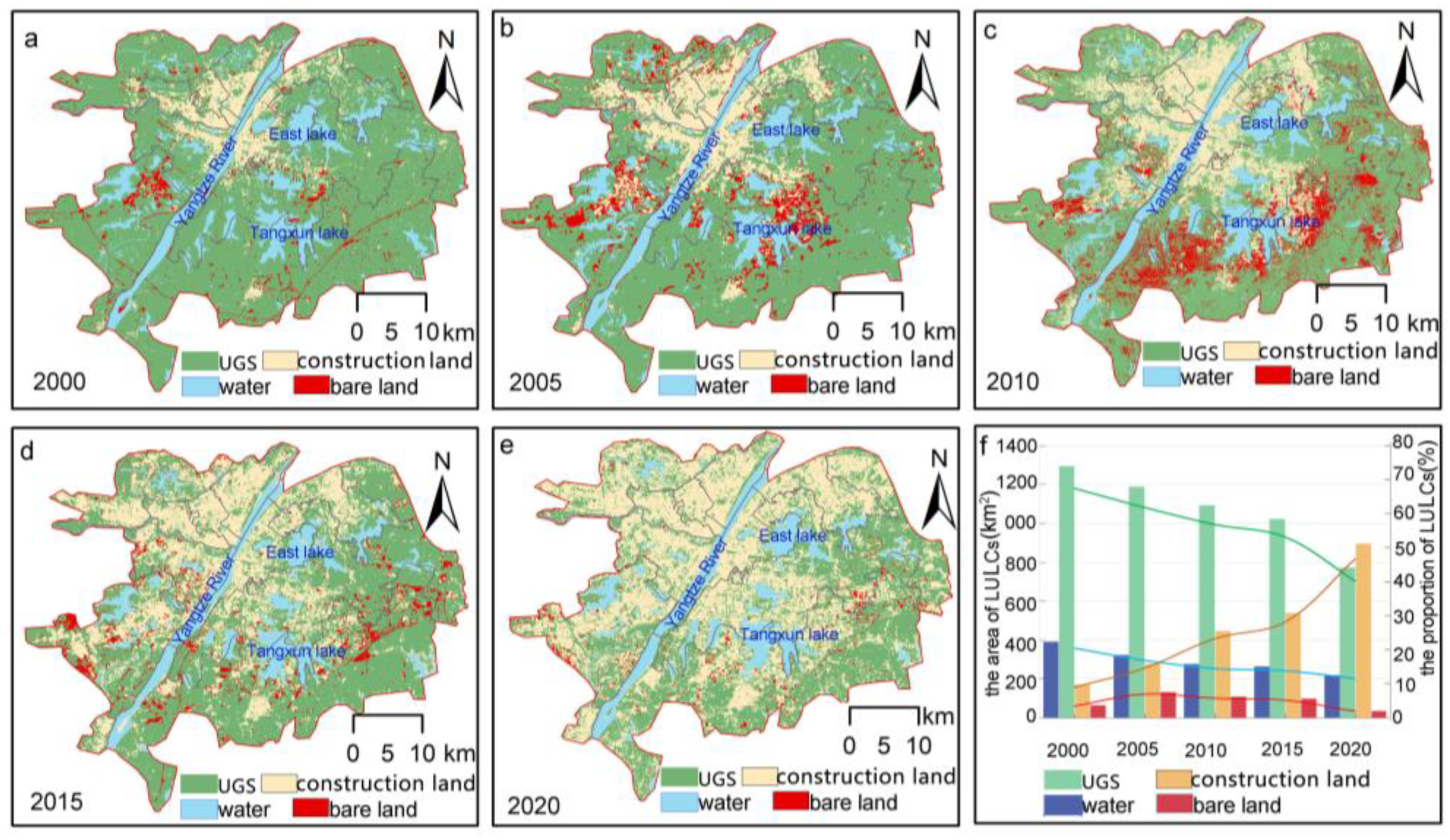
3.1.1. Spatiotemporal Evolution of LULC

From 2000 to 2020, the LULC experienced substantial fluctuations, with rates of 40.04%, 39.87%, 42.19%, and 44.19% in the four periods (Table S2a–d). The UGS area in the study region consistently declined, with a particularly sharp decrease from 2015 to 2020, during which the reduction rate was fourfold greater than that in the previous 15 years. This reduction predominantly extended southwards and eastwards (Figure 6a).

In terms of UGS expansion, the contributions of different LULC types varied over time (Figure 6b). Water bodies were the major contributors in the first period (2000–2005), accounting for 60.74% of the UGS expansion area. The efficiency of converting bare land to UGSs was consistently the highest throughout the period, with an average of 41.38%. Furthermore, the conversion area of bare land to UGS peaked in 2005–2010, comprising 42.67% of UGS growth. After 2010, the role of construction land in UGS expansion grew, surpassing 55% in the following decade.

The loss of UGSs was divided into two phases, mainly caused by bare land and construction land (Figure 6b). From 2000 to 2005, bare and construction land equally contributed to UGS loss, together accounting for more than 80% of the reduction. After 2005, construction land emerged as the dominant encroacher on UGSs and was responsible for approximately 60% of the total UGS reduction from 2005−2015 and 90% from 2015−2020.

Figure 7a shows that the conversion areas between the four LULCs exhibit significant global spatial autocorrelation characteristics (Z > 2.58), with a clustered distribution (Moran’s I > 0). Notably, from 2000 to 2020, areas in which other LULCs were converted to UGSs revealed a downwards trend in the clustering of water bodies and bare land, with Moran’s I values decreasing from 0.24 and 0.21 in 2000 to 0.09 and 0.12 in 2020. The degree of aggregation of converted spaces from construction land to UGS first decreased and then increased, reaching the lowest level in 2005−2010 (Moran’s I = 0.156). In contrast, for conversion spaces from UGSs to other LULCs, construction land consistently exhibited greater spatial closeness than did other land types, with conversions to bare land and water bodies reaching peak closeness in 2010−2015 (Moran’s I = 0.164).

In addition, the conversion areas between UGSs and other LULCs predominantly exhibit homogeneous spatial characteristics in HH and LL clusters, with some differences. Specifically, in the areas where other LULCs convert to UGSs, the HL clusters of construction land converting to UGSs significantly increased, reaching 11 blocks in 2010, while the conversion of bare land and water areas remained minimal (Figure 7b). In the HH clusters, the number of blocks where bare land converted to green space consistently increased from 2005 to 2020, reflecting continuous optimization of UGSs. In the areas where UGSs convert to other LULCs, the HH clusters of UGSs converting to bare land significantly increased after 2005. In the LL clusters, the number of blocks where UGSs converted to construction land and bare land consistently increased, indicating that concentrated development has a notable impact on green space degradation (Figure 7c).

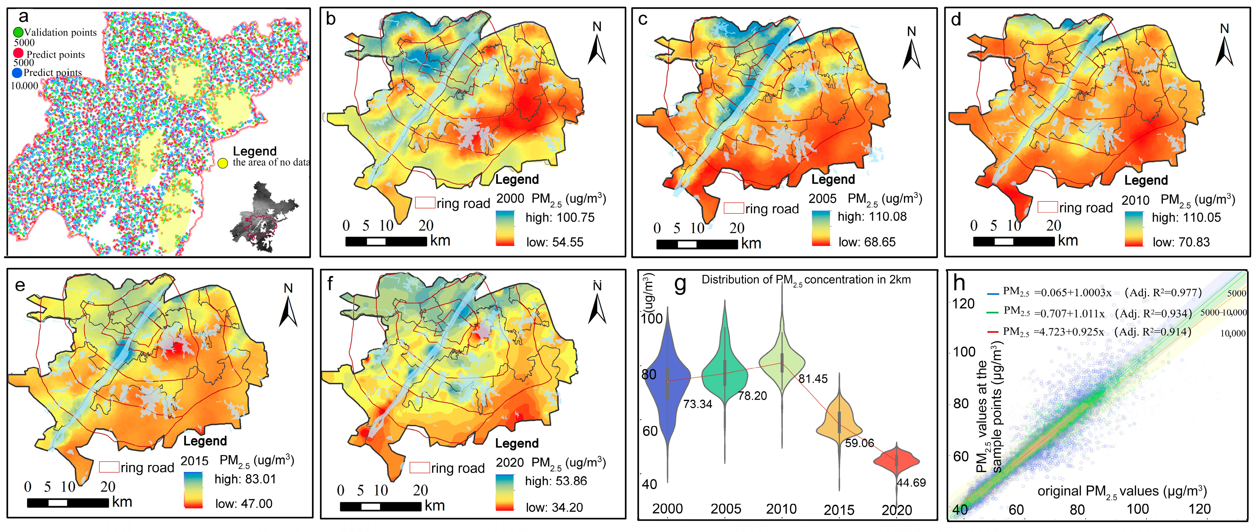
3.1.2. Spatiotemporal Evolution of the PM_2.5 Concentration and Its Fluctuations

From 2000 to 2020, the mean concentration of PM_2.5 initially increased and then decreased, peaking in 2010 and later falling to 44.81 μg/m³ in 2020, which was significantly higher than the WHO standard in 2021 (5 μg/m³). Spatially, the PM_2.5 concentration in the study area exhibited a pattern of being greater in the northwest and lower in the southeast (Figure 8a).

PM_2.5 pollution in the study area underwent a two-phase trend during the study period (Figure 8a). Initially, the concentrations generally increased, especially in the areas between the third and fourth ring roads, which serve as major urban expressways facilitating traffic flow in Wuhan. This region, along with the areas south of Tangxun Lake and northwest of East Lake, experienced significant pollution. However, in several western and southern regions, including areas northwest of the Yangtze River and East Lake, the emissions decreased (0–16.32 μg/m³) from 2000 to 2010. A marked turnaround occurred after 2010, with PM_2.5 levels dropping substantially across the area. This was particularly evident from 2010 to 2015, with declines reaching 40 μg/m³ near Tangxun Lake and East Lake, and it continued through 2015 to 2020, notably in the urban districts west of the Yangtze River. The overall trend reflects a progressive reduction in PM_2.5, moving from the outskirts to the city center.

Additionally, in terms of spatial autocorrelation, areas of PM_2.5 and its changes in the study area demonstrated strong global spatial autocorrelation (Moran’s I > 0.46, p < 0.001), with notable scale-dependent variations. Stronger spatial correlations were observed at smaller scales (1–2 km), especially compared to 3–5 km scales. However, spatial connections in areas of PM_2.5 and their differences at the 2 km scale were more pronounced than those at the 1 km scale. Locally, 30−40% of the area exhibited clustering in areas with different PM_2.5 concentrations, with the HH and LL patterns being particularly distinct (Figure 8b,c).

3.2. OLS Results

The influence of LULC conversion on PM_2.5 changes varied significantly across the four periods and scales (

Table 1. Global spatial relationships between UGS conversion area and PM_2.5 concentration changes at four scales.

Evolution Stages	Parameters	1 km × 1 km	2 km × 2 km	3 km × 3 km	5 km × 5 km
2000–2005	RSS	1632.67	374.83	169.45	46.80
	AIC	4846.75	1179.28	534.24	187.42
	R2	0.06	0.13	0.11	0.32
	Adj.R2	0.06	0.12	0.08	0.26
2005–2010	RSS	1635.04	389.04	171.24	52.20
	AIC	4849.28	1195.32	536.24	194.96
	R2	0.06	0.10	0.10	0.24
	Adj.R2	0.06	0.09	0.07	0.17
2010–2015	RSS	1474.13	266.59	166.44	68.60
	AIC	4668.81	1032.41	530.84	213.81
	R2	0.15	0.38	0.12	0.01
	Adj.R2	0.15	0.37	0.10	-
2015–2020	RSS	1565.56	226.46	140.44	53.33
	AIC	4773.63	962.10	498.57	196.43
	R2	0.10	0.48	0.26	0.23
	Adj.R2	0.10	0.47	0.24	0.15

). The influence of UGS conversion on the model fit quality for PM_2.5 changes shows considerable changes across the scales. Particularly in the second period (2005–2010), this influence intensifies with increasing scale, yet the most pronounced R² values are consistently observed at the 2 km scale in other periods. Specifically, the first period demonstrated an “increase–decrease–increase” pattern with increasing scale. In contrast, in the third and fourth periods, the models at the 2 km scale exhibit the highest fitting accuracy, with their influence diminishing as the scale increases. Additionally, at the 2 km and 3 km scales, the fourth period and the second period showcase the best and the poorest model fits, respectively, with R² values of 0.475 and 0.261 and 0.097 and 0.099, respectively. At the 1 km and 5 km scales, the highest R² values are noted in the third period (R² = 0.154) and the first period (R² = 0.332), with the lowest being in the second period (R² = 0.061) and the third period (R² = 0.006).

3.3. MGWR Results

3.3.1. The MGWR Model Exhibits Better Performance

Table 2. Local spatial relationships between the UGS conversion area and PM_2.5 changes at four scales.

Evolution Stages	Parameters	1 km × 1 km		2 km × 2 km		3 km × 3 km		5 km × 5 km
		GWR	MGWR	GWR	MGWR	GWR	MGWR	GWR	MGWR
2000–2005	Bandwidths	300.00	-	56.00	-	85.00	-	65.00	-
	RSS	896.21	169.58	136.84	128.93	89.06	70.48	30.10	23.31
	AIC	3970.48	2791.23	1003.89	927.07	473.08	428.71	174.05	166.44
	R2	0.49	0.90	0.68	0.70	0.53	0.629	0.564	0.66
	Adj.R2	0.46	0.85	0.58	0.62	0.44	0.556	0.462	0.56
2005–2010	Bandwidths	300.00	-	62.00	-	65.00	-	65.00	-
	RSS	937.60	334.06	159.51	127.09	82.64	71.96	38.86	31.51
	AIC	4045.95	2888.04	1044.57	945.68	488.46	451.27	192.96	185.36
	R2	0.46	0.81	0.63	0.71	0.57	0.62	0.44	0.54
	Adj.R2	0.43	0.76	0.52	0.62	0.45	0.53	0.3	0.41
2010–2015	Bandwidths	300.00	-	80.00	-	78.00	-	57.00
	RSS	572.58	318.18	144.39	124.28	92.84	81.45	42.67	33.13
	AIC	3192.19	2672.58	944.04	884.76	488.65	473.00	205.83	194.73
	R2	0.67	0.82	0.67	0.71	0.51	0.57	0.38	0.52
	Adj.R2	0.65	0.78	0.59	0.65	0.41	0.47	0.20	0.36
2015–2020	Bandwidths	300.00	-	67.00	-	69.00	-	68.00	-
	RSS	544.74	326.03	107.52	86.70	74.76	61.76	46.68	35.95
	AIC	3102.13	2612.38	853.78	765.23	459.56	410.95	202.14	194.36
	R2	0.69	0.81	0.75	0.80	0.61	0.68	0.324	0.45
	Adj.R2	0.67	0.78	0.69	0.75	0.51	0.61	0.18	0.33

indicates that the MGWR model more effectively reveals the local spatial relationship between PM_2.5 and UGS conversion than does the GWR model because of the higher R² values and lower RSS and AIC values at all stages and scales. However, the fit of the local regression model varies with geographical scale and evolutionary stage. (1) Concerning the geographical scale, the best fits at 1 km and 5 km were noted in the first stage (R² = 0.903 and 0.662, respectively), with a subsequent gradual decline in fit as the UGSs evolved. At 2 km and 3 km, the fit initially decreased and then increased, reaching the highest significance in the fourth stage (R² = 0.799 and 0.675, respectively). (2) Regarding evolutionary stages, generally, the MGWR fit decreased with increasing scale, yet the fit at the 5 km scale in the first stage (R² = 0.662) was slightly better than that at 3 km (R² = 0.629).

3.3.2. The UGS Conversion Space Shows Unstable Spatial Variable Properties

Additionally, the MGWR results demonstrated significant variability in scale estimation (bandwidth: 43–1741) for LULC conversion areas across different scales and stages (

Table 3. Bandwidths of the conversion area of UGSs to/from the other three LULCs at the four scales in the MGWR.

Evolution Stages	Scales	Intercept	1 → 2	1 → 3	1 → 4	2 → 1	3 → 1	4 → 1
2000–2005	1 km	46	376	1741	64	53	539	112
	2 km	43	69	43	212	64	430	45
	3 km	43	177	182	94	138	44	162
	5 km	48	48	46	65	48	67	67
2005–2010	1 km	43	253	46	146	70	44	70
	2 km	43	43	216	46	55	430	44
	3 km	44	99	55	82	45	189	133
	5 km	46	46	52	67	67	67	65
2010–2015	1 km	43	46	364	100	480	46	176
	2 km	43	409	60	52	57	430	99
	3 km	45	79	62	189	102	72	49
	5 km	44	44	67	67	44	48	44
2015–2020	1 km	43	1734	46	1741	411	72	331
	2 km	43	430	44	428	99	44	47
	3 km	45	189	48	189	189	45	189
	5 km	53	67	52	44	53	67	67

Note: 1 → 2 = UGS is converted into water, 1 → 3 = UGS is converted into construction land, 1 → 4 = UGS is converted into bare land, and 2 → 1, 3 → 1, and 4 → 1 are the opposite.

). This suggests that UGS conversion areas exhibit unstable spatial variable attributes (global and/or local). For instance, in the fourth stage, the areas where UGSs were converted to water bodies represented a global spatial variable at all scales (bandwidths: 1734, 430, 189, and 67), indicating that a global spatial model (OLS) could more accurately explain the spatial relationship of such LULC conversions with PM_2.5, in this case. Conversely, water bodies converted to UGSs exhibited relatively stable local spatial variable attributes at four stages, except for the second stage at 5 km (bandwidth: 67) and the fourth stage at 3 km (bandwidth: 189). However, the GWR analysis for the six types of LULC conversion areas and PM_2.5 showed a uniform bandwidth value (Table 2). Therefore, relying solely on GWR analysis may yield inaccurate results, while MGWR provides a more precise explanation of the spatial heterogeneity impact of UGS conversion on PM_2.5 concentration changes.

3.3.3. The 2 km Scale Is a Scientific Scale for Examining Local Spatial Relationships

Overall, the 2 km scale emerges as a pragmatic choice for examining the spatial heterogeneity between UGS conversion and PM_2.5 fluctuations in the study area, for three reasons. (1) At 1 km and 2 km, the MGWR revealed more significant local spatial variable attributes in UGS conversion areas (Table 3), and the global and local spatial correlations of PM_2.5 and its changes were more pronounced (Table 2), thereby effectively capturing the spatial heterogeneity relationship between UGS conversion areas and PM_2.5 changes. (2) Compared to those obtained with the 1 km resolution, the models obtained with both GWR and MGWR at the 2 km scale demonstrated greater explanatory power, indicating more stable local regression outcomes within this study area at the 2 km scale (Table 2). (3) At the 2 km scale, focusing only on UGS conversion and excluding other LULC-type conversions, such as water and construction land, the conversion of UGSs accounted for more than 70% of the PM_2.5 changes in all study stages, as shown by high R² values (R² > 0.7) (Table 2). This indicates the importance of analyzing UGS conversions at the 2 km scale, as these transformations significantly impacted the observed changes in PM_2.5 concentrations.

3.4. Spatial Heterogeneity Impact of UGS Conversion on PM_2.5 Changes at the 2 km Scale

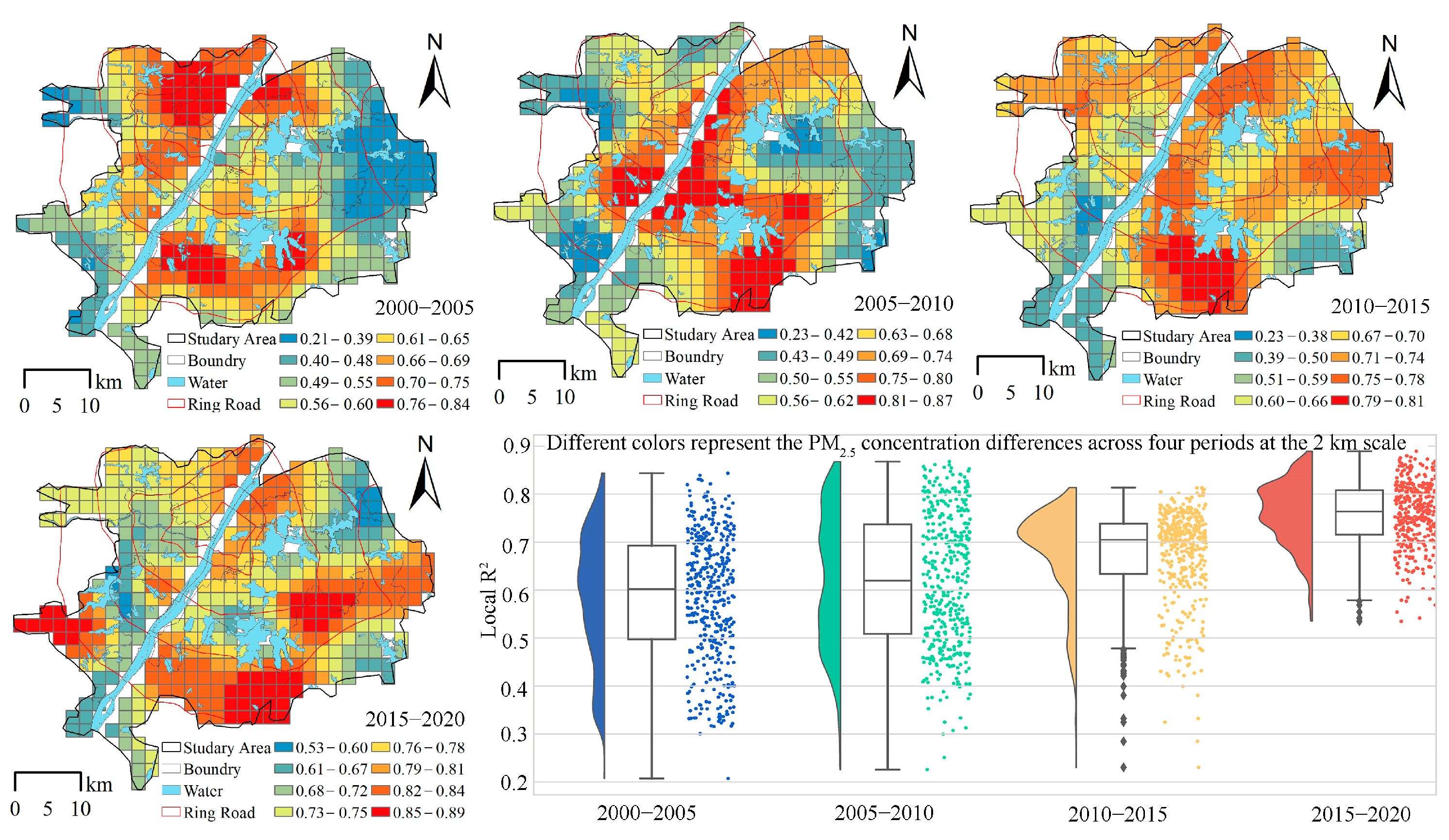
3.4.1. Spatiotemporal Pattern of the Local R² Values

From 2000 to 2020, a dynamic shift was observed in the correlation between UGS conversion and PM_2.5 concentration variability, as evidenced by evolving local R² values (Figure 9, Table S3). UGS conversions, on average, were found to explain 64.75% of the PM_2.5 concentration variances within the study area, demonstrating a progressively strengthening influence throughout this period. Notably, the explanatory power peaked at 76.4% in 2015–2020, underscoring the increasingly pivotal role of UGSs in modulating PM_2.5 levels. This contrasts with the 2000–2005 period, where lower R² values suggest a more intricate array of factors influencing PM_2.5 concentrations. A significant increase in areas where UGS conversions explained more than 60% of the total PM_2.5 fluctuations was observed across the four stages, occupying 51.04%, 52.67%, 83.06%, and 98.38% of the study area, respectively. This finding underscores the increasingly pronounced interrelationship between UGS quantity and spatial structure and PM_2.5 concentration dynamics, particularly after 2010.

Throughout the four stages, the spatial pattern of the influence of UGS conversion on PM_2.5 change, represented by local R² values, transitioned from northwest to southeast (Figure 9). This reflects a shift from a dispersed to a concentrated impact on PM_2.5 concentrations between 2000 and 2015, followed by redispersion in 2020. In the third stage, regions exhibiting stronger correlations with PM_2.5 variations were densely aggregated, revealing a uniform spatial response. Conversely, during the fourth stage, these influential areas spread out, mainly between the fourth and outer ring roads in the southern and eastern regions of East and Tangxun Lakes. Predominantly, the UGS areas south of Tangxun Lake consistently exhibited a strong correlation with PM_2.5 fluctuations throughout all the stages, in contrast to the consistently lower correlation in the southern regions of the Caidian and Jiangxia districts.

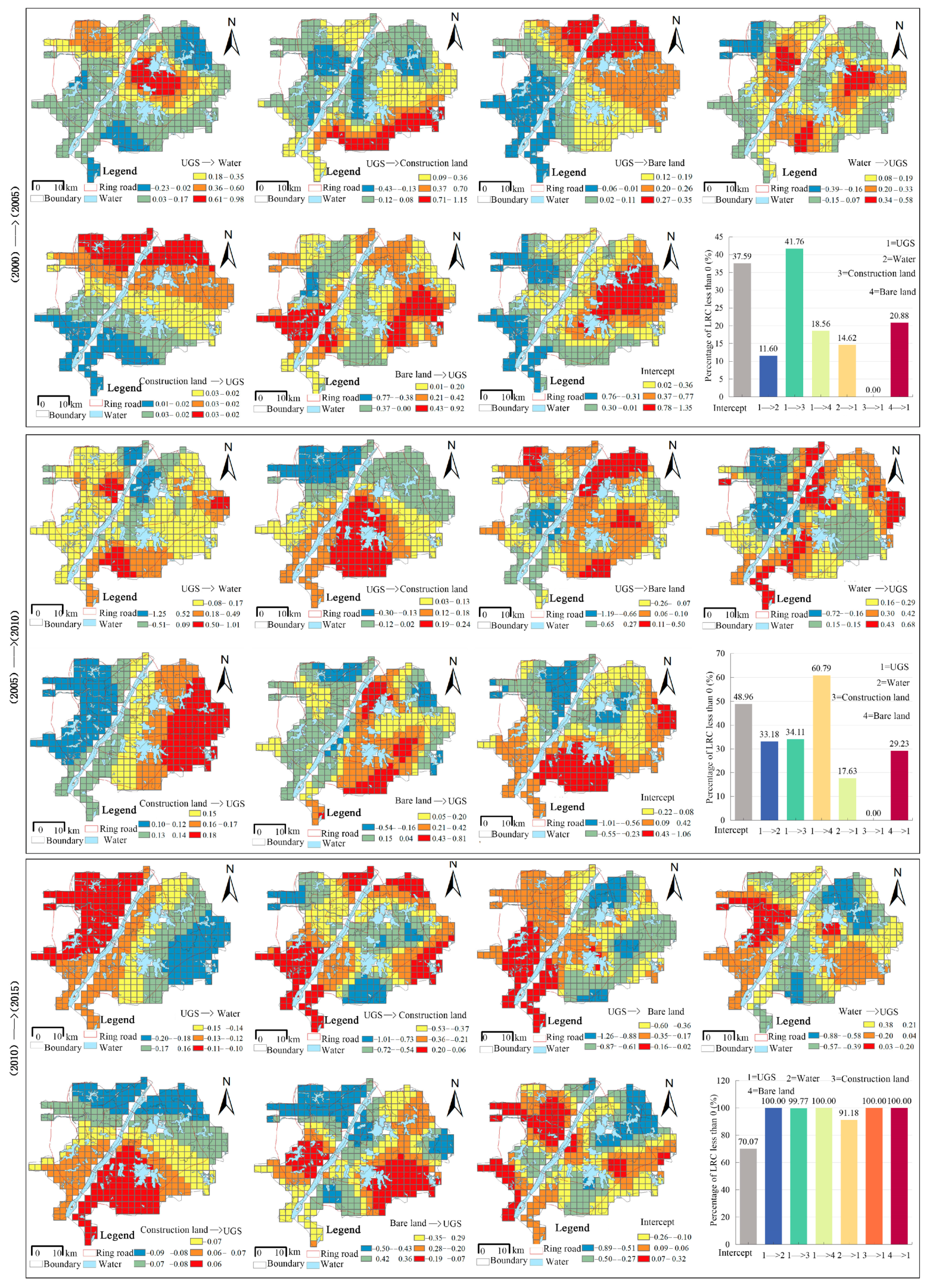
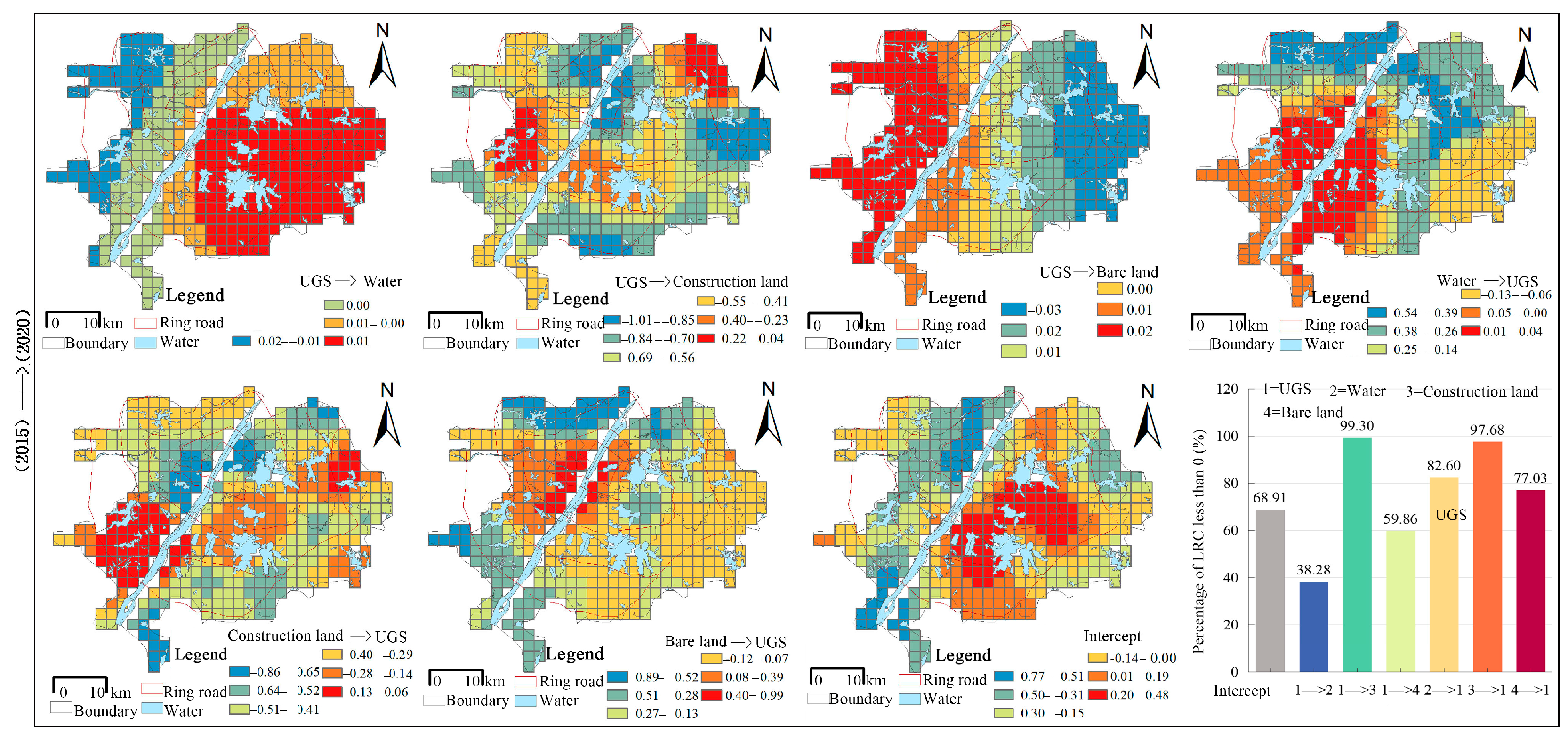
3.4.2. Spatiotemporal Pattern of LRCs between UGS Conversion and PM_2.5 Changes

The LRCs elucidated the complex relationship between UGS conversion and changes in PM_2.5 levels across the four stages, highlighting the varied impacts of LULC changes (Figure 10). LRC values less (more) than 0 reflect a negative (positive) correlation between UGSs conversion areas and PM_2.5 concentrations, with larger absolute values (|LRC|) indicating a more pronounced effect in mitigating PM_2.5 pollution.

The impacts of UGS conversion on PM_2.5 are multifaceted and differ by period and location. For instance, UGS conversion to/from other LULCs has positive and negative effects on PM_2.5 concentrations, illustrating spatial variability. Specifically, (1) UGS conversion to/from other LULCs consistently had both positive and negative effects on the PM_2.5 concentration across all four stages, indicating obvious spatial heterogeneity in the impact of UGS conversion on PM_2.5. This proves that when UGSs reach a certain area, the key to effectively mitigating PM_2.5 pollution is to determine the specific location of the UGS. (2) Different LULC transformations impact PM_2.5 levels variably within the same period. For instance, during the period from 2000 to 2005, approximately 88.4% and 81.44% of the areas, especially around Tangxun Lake, East Lake, and the Caidian District, exhibited more severe PM_2.5 pollution when UGSs were converted to water bodies and bare land, respectively (LRC > 0). Conversely, UGSs that changed to construction land (58.24% with LRC > 0) were mostly west of the Yangtze River and along its east bank. Moreover, in regions with LRCs less than 0, converting bare land to UGSs (|LRC|max = 0.77) was most effective at reducing PM_2.5, especially in southern parts of the study area, including the Caidian and Jiangxia Districts. Taken together, these findings show that in these regions, restoring bare land to UGSs is more effective at mitigating PM_2.5 pollution than restoring other LULCs. (3) Temporal variations distinctly modulate the impact of identical UGS transformations on PM_2.5 concentrations. For example, in the context of UGS conversion to construction land, 58.24% of the area demonstrated a positive correlation (LRC > 0) with elevated PM_2.5 levels in 2000–2005, which increased to 65.89% in 2005–2010. Regarding the magnitude of impact, this LULC transition exhibited the most pronounced increase in PM_2.5 from 2000–2005, as indicated by the highest recorded LRC value of 1.15. This spatiotemporal variation in impact underscores the need for tailored UGS optimization strategies to address PM_2.5 changes effectively.

4. Discussion

This study adopts a longitudinal dynamic-evolution analysis perspective to effectively reduce the interference of geographical environmental differences [57], providing deeper insight into the relationship between LULC change and PM_2.5 concentration. Using Wuhan as the study area, we proposed an innovative practical framework for analyzing how coordinated LULC optimization can address environmental pollution issues. This framework has several key advantages.

4.1. Practical Guidance: Multifaceted Spatiotemporal LULC Transformations

Our framework focuses on the conversion of UGSs to/from other LULC types and plays a significant role in practical planning guidance. Previous studies predominantly linked UGS quantity and morphology with PM_2.5, suggesting that UGS modulation is a solution for alleviating PM_2.5 pollution. These studies generally suggest that increasing construction land and water bodies escalate PM_2.5 concentrations, whereas UGSs reduce PM_2.5 concentrations [22,59,60]. However, our findings argue that this trend is not consistent across scales and periods. For instance, UGS-to-construction land conversions, particularly in Jiangxia District (2000–2010), do not consistently align with PM_2.5 reductions across four periods and settings (Figure 9). This inconsistency highlights the limitations of generalizing UGS impacts, especially in high-density urban areas with scarcer land resources [12] and relatively stable spatial structures. This is because in the process of urban spatial planning, changes in one LULC must correspond to changes in another (several) LULC(s).

Therefore, our study emphasizes the need for tailored spatial strategies and precise scale optimization. By the new framework proposed through spatiotemporal evolution and collaborative optimization of LULCs, we establish that UGS modifications yield variable impacts on PM_2.5 levels that are dependent on specific spatiotemporal contexts and scales (Section 4.3.1). For instance, at 2 km scales, in Dongxihu, Caidian, and Jiangxia districts (2015–2020), UGS-to-construction land conversion most effectively reduced PM_2.5 (|LRC| = 1.01; Figure 9); however, in the Fuhuan River and Jinyin Lake areas, optimizing water bodies and bare land was more beneficial. These insights underscore the importance of context-specific LULC-optimizing strategies in PM_2.5 management, transcending simplistic assumptions about UGS effects and revealing more significant practical characteristics.

4.2. Essential Analysis: Diagnosing Spatial Variable Properties and Research Scales

Studying the UGS-PM_2.5 relationship and spatially continuous variables often involves comparing global and local spatial models. While earlier studies, such as Li et al., (2010) and Bi et al., (2022b), typically found GWR to have superior R² values [21,27], our research indicates a shift in this pattern beyond a 2 km scale. Specifically, during 2000–2010, the advantages of the GWR model for mapping the spatial dynamics between UGS conversion and PM_2.5 changes decreased. For instance, between 2005 and 2010, the R² values that captured OLS and GWR increased (decreased) from 0.097 (0.63) to 0.244 (0.43), respectively (Table 1 and Table 2), suggesting the limited applicability of static models at various scales. Our study introduces the MGWR model, which reveals both global and local spatial variable properties of conversion areas between UGSs and other LULCs at different scales (2000–2020; Table 3). For example, in 2000–2005, the space to which UGSs are converted to water bodies presented a global spatial variable at the 3 km scale (bandwidth: 177), yet it demonstrated local spatial variability at the other three scales (bandwidths: 376, 69, and 48). This indicates the enhanced ability of the MGWR to delineate spatial heterogeneity in the dynamic interplay between UGSs and PM_2.5, underscoring the importance of scale in spatial analysis.

Through OLS, GWR, and MGWR, we established that scale diagnosis is integral to understanding the spatial heterogeneity in UGS and PM_2.5 changes from 2000 to 2020 across 1–5 km scales. A 2 km scale emerged as optimal for examining UGS-PM_2.5 spatial heterogeneity in our region (Section 3.3.2), leading to a multidimensional strategy for UGS–LULC-related PM_2.5 mitigation (Section 4.3). These findings support comprehensive multiscale spatiotemporal analysis in UGS spatial regression research, cautioning against the limitations of fixed spatiotemporal scopes and ignoring the spatial variable characteristics of research objects.

4.3. Multidimensional Strategy: UGS-LULC Synergy for PM_2.5 Mitigation

Our multidimensional strategy extends beyond typical LULC optimization, employing insights from the MGWR on spatial heterogeneity to prioritize and localize diverse LULC interventions within the study area. The period 2015–2020 exemplifies our approach, where synergistic optimization of UGSs and other LULCs was used to address PM_2.5 challenges effectively.

In this context, MGWR analysis informs our decisions by highlighting the strongest PM_2.5 mitigators in local 2 km grids, such as bare land (|LRC| = 0.89), construction land (|LRC| = 0.86), and water bodies (|LRC| = 0.54). Notably, UGS restoration in construction zones emerges as a key strategy, potentially impacting more than 90% of the area (Figure 9). Thus, prioritizing construction land for UGS transformation, followed by bare land and water bodies, becomes crucial.

4.3.1. Synergistic Strategy for UGS and Construction Land

The UGS–construction-land synergistic strategies aimed at reducing PM_2.5 are complex, due to spatial differences. A detailed examination revealed that in high-density urban areas such as the northwestern East Lake and Jianghan, Qiaokou, and Hanyang Districts, the two LULC conversions significantly impacted PM_2.5 changes (LRC: −0.65 to −0.89), highlighting these as key areas for UGS enhancement. The augmentation of smaller UGS units, such as street gardens, within these 2 km scales, or the linking of existing small UGSs to form larger UGS entities is crucial for reducing PM_2.5. In contrast, the southern and eastern peripheries of Tangxun Lake, encompassing areas of Qiaokou and Hanyang Districts and the northwestern section of Jianghan District, exhibited moderate impacts of LULC conversions on PM_2.5 (LRC: −0.41–−0.64). In these locations, optimization should focus on strengthening the peripheral green belts around Tangxun Lake and improving the green belt in the transition area between the large UGS patch and the construction land.

4.3.2. UGS Strategy with Bare Land and Water

Prioritizing UGS and bare land optimization, particularly in districts such as Qingshan, Dongxihu, Caidian, and Jiangxia, as well as in the area between East Lake and South Lake (LRC: −0.30–−0.89), is crucial. Linking larger UGS patches and restoring bare land can substantially reduce PM_2.5 concentrations. Similarly, optimizing UGSs alongside water bodies, especially around the Fuhuan River, Jinyin Lake, East Lake, and Tangxun Lake (LRC: −0.38–−0.54), involves restoring large UGS patches and transitional protection green belts around these water bodies, especially near Jinyin Lake, significantly lowering PM_2.5 levels. Strengthening the protection of lakes and rivers to the west of East Lake and Tangxun Lake, such as Houguan Lake and Nantaizi Lake, preventing farmland encroachment, and enhancing water connectivity projects, are crucial for improving air quality [61].

In summary, our synergistic strategies involving UGSs and other LULCs, which are tailored for different periods and locations, not only optimize UGSs but also align other LULCs for effective PM_2.5 reduction. For instance, according to Zeng et al., (2018), judicious planning of LULC in the vicinity of urban water bodies is crucial for enhancing air quality [62]. On this basis, we further discussed how to optimize the LULC layout around water areas, especially for PM_2.5 emission reduction. This approach not only aims to lower PM_2.5 levels but also contributes to the conservation of water bodies in various parts of the study area, aligning with the broader goals of environmental protection.

5. Conclusions

This study aimed to elucidate the role of optimized UGSs in alleviating PM_2.5 pollution through pragmatic urban planning. We developed an integrated framework for harmonizing UGSs and other LULC transformations, targeting environmental challenges such as PM_2.5; the key advantages of this framework are detailed in Section 4.

The specific contributions of this research are as follows. (1) From 2000 to 2020, the LULC underwent substantial changes, exhibiting average fluctuations above 40%. During this process, the efficiency of converting bare land to UGS increased, with an average of 41.38% of the reduced area being transformed into UGS, providing a new understanding of the transformation relationship between LULCs. The spatial distribution of PM_2.5 concentrations and changes in PM_2.5 concentrations exhibited significant global spatial autocorrelation (Moran’s I > 0, p < 0.001), primarily manifested as HH and LL clusters in local spatial analysis. (2) Based on the unstable bandwidth values of the area of UGSs to/from the other three LULCs, it was proven that the conversion areas exhibit varying spatial properties (global or local spatial variables) across four scales and different evolution periods. Areas of UGSs from water demonstrated consistently stable local spatial properties at all scales throughout the study period. In contrast, the spatial properties of the other LULC transformations were found to be less consistent. (3) A multiscale comparison approach was proposed to capture the potential relationships between LULC transformations and spatially continuous variables. Focusing on PM_2.5 as a case study, we found that local spatial regression models (MGWR) provided a more detailed understanding (reflected in higher R² values) of the complex interplay between UGS conversions and PM_2.5 fluctuations than did the OLS models. However, this advantage generally decreased with increasing scale. We proposed, and validated the fact, that both global and local spatial analysis have an optimal scale of effectiveness. Specifically, a 2 km scale emerged as the most suitable for probing the spatial heterogeneity relationship between UGS transformations and PM_2.5 variations in the study area. At this defined scale, UGS conversions were found to account for approximately 64.75% of the PM_2.5 changes, with areas exhibiting local R² values above 70% predominantly shifting from the northwest to southeast regions. (4) The spatial conversions of UGS to/from the other three LULCs all exhibited stable positive and negative effects on the changes in PM_2.5 across the four stages. Employing the MGWR, we delineated the spatial heterogeneity impact of UGS conversion on PM_2.5 changes at the 2 km scale. Drawing from these results, we developed multidimensional UGS-LULC synergy optimization strategies, illustrated using the 2015–2020 period. These strategies demonstrated that modifying the spatial location of UGSs (i.e., the conversion between UGSs and different LULCs) could variably reduce PM_2.5 pollution. Additionally, this approach enabled specific temporal (when), scale-based (where), and spatial (how) diagnoses of how to synergistically optimize UGS and other LULC strategies for mitigating PM_2.5 pollution.

Despite these significant advancements, further detailed exploration of key areas is still needed. LULC classification requires finer refinement, especially since our analysis, which used 15 m resolution imagery, revealed the intricate impact of UGS transitions on PM_2.5 changes. Given the diversity of UGSs, such as grasslands and forests, higher-resolution remote sensing and a finer classification of LULC patterns are essential for obtaining an in-depth understanding of their interactions with PM_2.5. Future studies should also investigate the collective effects of various LULC transitions on PM_2.5, aiming for more accurate results. Additionally, considering the seasonal variability in PM_2.5 concentrations, extending the framework to analyze the impacts of UGS conversion on seasonal and monthly variations in PM_2.5 is vital. Finally, although the framework primarily addresses spatially continuous variables such as PM_2.5, exploring its applicability to non-spatially continuous variables is a promising direction for future research.

Nevertheless, an innovative framework was developed from a dynamic evolution perspective, employing multiscale comparisons through global and local spatial regression models to identify the optimal scale for analyzing the impact of UGS conversions on PM_2.5 pollution. Consequently, different LULCs were proposed to be synergistically optimized with UGS layouts to mitigate PM_2.5 pollution in high-density urban areas. Based on this, a multiscale spatiotemporal analysis framework was developed to formulate LULC synergy optimization strategies to address environmental issues such as PM_2.5, urban heat islands, and carbon emissions. This framework, due to the consideration of multiple LULC synergy optimizations, holds greater practical guidance value and significantly enhances the management and planning strategies for UGS and other LULCs (such as water bodies). This innovative framework allows for more precise LULCs diagnosis and optimization, thereby effectively improving air pollution and other environmental issues, demonstrating its significant potential in enhancing urban environmental management practices.

References

1. Shahtahmassebi, A.R.; Li, C.; Fan, Y.; Wu, Y.; Lin, Y.; Gan, M.; Wang, K.; Malik, A.; Blackburn, G.A. Remote Sensing of Urban Green Spaces: A Review. Urban For. Urban Green. 2021, 57, 126946. [Google Scholar] [CrossRef]
2. World Health Organization (WHO). New WHO Global Air Quality Guidelines Aim to Save Millions of Lives from Air Pollution. Available online: https://www.who.int/news/item (accessed on 25 November 2023).
3. Lu, F.; Xu, D.Q.; Cheng, Y.B.; Dong, S.X.; Guo, C.; Jiang, X.; Zheng, X.Y. Systematic Review and Meta-Analysis of the Adverse Health Effects of Ambient PM2.5 and PM10 Pollution in the Chinese Population. Environ. Res. 2015, 136, 196–204. [Google Scholar] [CrossRef] [PubMed]
4. Hu, Z. Spatial Analysis of MODIS Aerosol Optical Depth, PM2.5, and Chronic Coronary Heart Disease. Int. J. Health Geogr. 2009, 8, 27. [Google Scholar] [CrossRef] [PubMed]
5. Kwag, Y.; Kim, M.H.; Oh, J.; Shah, S.; Ye, S.; Ha, E.H. Effect of Heat Waves and Fine Particulate Matter on Preterm Births in Korea from 2010 to 2016. Environ. Int. 2021, 147, 106239. [Google Scholar] [CrossRef]
6. Coccia, M. Effects of the Spread of COVID-19 on Public Health of Polluted Cities: Results of the First Wave for Explaining the Deja Vu in the Second Wave of COVID-19 Pandemic and Epidemics of Future Vital Agents. Environ. Sci. Pollut. Res. 2021, 28, 19147–19154. [Google Scholar] [CrossRef]
7. Paital, B.; Agrawal, P.K. Air Pollution by NO2 and PM2.5 Explains COVID-19 Infection Severity by Overexpression of Angiotensin-Converting Enzyme 2 in Respiratory Cells: A Review. Environ. Chem. Lett. 2021, 19, 25–42. [Google Scholar] [CrossRef] [PubMed]
8. Zhu, Y.J.; Xie, J.G.; Huang, F.M.; Cao, L.Q. Association between Short-Term Exposure to Air Pollution and COVID-19 Infection: Evidence from China. Sci. Total Environ. 2020, 727, 138704. [Google Scholar] [CrossRef] [PubMed]
9. Cai, L.; Zhuang, M.; Ren, Y. Spatiotemporal Characteristics of NO2, PM2.5 and O3 in a Coastal Region of Southeastern China and Their Removal by Green Spaces. Int. J. Environ. Health Res. 2022, 32, 1–17. [Google Scholar] [CrossRef] [PubMed]
10. Chen, M.; Dai, F.; Yang, B.; Zhu, S. Effects of Urban Green Space Morphological Pattern on Variation of PM2.5 Concentration in the Neighborhoods of Five Chinese Megacities. Build. Environ. 2019, 158, 1–15. [Google Scholar] [CrossRef]
11. Chen, L.X.; Liu, C.M.; Zou, R.; Yang, M.; Zhang, Z.Q. Experimental Examination of Effectiveness of Vegetation as Bio-Filter of Particulate Matters in the Urban Environment. Environ. Pollut. 2016, 208, 198–208. [Google Scholar] [CrossRef]
12. Li, Y.; Zhang, Y.; Wu, Q.; Xue, R.; Wang, X.; Si, M.; Zhang, Y. Greening the Concrete Jungle: Unveiling the Co-Mitigation of Greenspace Configuration on PM2.5 and Land Surface Temperature with Explanatory Machine Learning. Urban For. Urban Green. 2023, 88, 128086. [Google Scholar] [CrossRef]
13. Cai, L.Y.; Zhuang, M.Z.; Ren, Y. A Landscape Scale Study in Southeast China Investigating the Effects of Varied Green Space Types on Atmospheric PM2.5 in Mid-Winter. Urban For. Urban Green. 2020, 49, 126607. [Google Scholar] [CrossRef]
14. Qiu, L.; Liu, F.; Zhang, X.; Gao, T. Difference of Airborne Particulate Matter Concentration in Urban Space with Different Green Coverage Rates in Baoji, China. Int. J. Environ. Res. Public Health 2019, 16, 1465. [Google Scholar] [CrossRef] [PubMed]
15. Moniruzzaman, M.; Thakur, P.K.; Kumar, P.; Ashraful Alam, M.; Garg, V.; Rousta, I.; Olafsson, H. Decadal Urban Land Use/Land Cover Changes and Its Impact on Surface Runoff Potential for the Dhaka City and Surroundings Using Remote Sensing. Remote Sens. 2021, 13, 83. [Google Scholar] [CrossRef]
16. Lu, Y.; Yang, X.; Wang, H.; Jiang, M.; Wen, X.; Zhang, X.; Meng, L. Exploring the Effects of Land Use and Land Cover Changes on Meteorology and Air Quality over Sichuan Basin, Southwestern China. Front. Ecol. Evol. 2023, 11, 1131389. [Google Scholar] [CrossRef]
17. Li, M.; Song, Y.; Mao, Z.; Liu, M.; Huang, X. Impacts of Thermal Circulations Induced by Urbanization on Ozone Formation in the Pearl River Delta Region, China. Atmos. Environ. 2016, 127, 382–392. [Google Scholar] [CrossRef]
18. Javaid, K.; Ghafoor, G.Z.; Sharif, F.; Shahid, M.G.; Shahzad, L.; Ghafoor, N.; Farhan, M. Spatio-Temporal Analysis of Land Use Land Cover Change and Its Impact on Land Surface Temperature of Sialkot City, Pakistan. Sci. Rep. 2023, 13, 22166. [Google Scholar] [CrossRef] [PubMed]
19. Yousefi, R.; Shaheen, A.; Wang, F.; Ge, Q.; Wu, R.; Lelieveld, J.; Wang, J.; Su, X. Fine Particulate Matter (PM2.5) Trends from Land Surface Changes and Air Pollution Policies in China during 1980–2020. J. Environ. Manag. 2023, 326, 116847. [Google Scholar] [CrossRef]
20. Zhang, P.; Ma, W.; Wen, F.; Liu, L.; Yang, L.; Song, J.; Wang, N.; Liu, Q. Estimating PM2.5 Concentration Using the Machine Learning GA-SVM Method to Improve the Land Use Regression Model in Shaanxi, China. Ecotoxicol. Environ. Saf. 2021, 225, 112772. [Google Scholar] [CrossRef]
21. Bi, S.; Dai, F.; Chen, M.; Xu, S. A New Framework for Analysis of the Morphological Spatial Patterns of Urban Green Space to Reduce PM2.5 Pollution: A Case Study in Wuhan, China. Sustain. Cities Soc. 2022, 82, 103900. [Google Scholar] [CrossRef]
22. Li, K.; Li, C.; Hu, Y.; Xiong, Z.; Wang, Y. Quantitative Estimation of the PM2.5 Removal Capacity and Influencing Factors of Urban Green Infrastructure. Sci. Total Environ. 2023, 867, 161476. [Google Scholar] [CrossRef] [PubMed]
23. Mo, Y.; Booker, D.; Zhao, S.; Tang, J.; Jiang, H.; Shen, J.; Chen, D.; Li, J.; Jones, K.C.; Zhang, G. The Application of Land Use Regression Model to Investigate Spatiotemporal Variations of PM2.5 in Guangzhou, China: Implications for the Public Health Benefits of PM2.5 Reduction. Sci. Total Environ. 2021, 778, 146305. [Google Scholar] [CrossRef] [PubMed]
24. Ouyang, W.; Gao, B.; Cheng, H.; Hao, Z.; Wu, N. Exposure Inequality Assessment for PM2.5 and the Potential Association with Environmental Health in Beijing. Sci. Total Environ. 2018, 635, 769–778. [Google Scholar] [CrossRef] [PubMed]
25. Yang, H.O.; Chen, W.B.; Liang, Z.F. Impact of Land Use on PM2.5 Pollution in a Representative City of Middle China. Int. J. Environ. Res. Public Health 2017, 14, 462. [Google Scholar] [CrossRef]
26. Li, K.; Li, C.; Liu, M.; Hu, Y.; Wang, H.; Wu, W. Multiscale Analysis of the Effects of Urban Green Infrastructure Landscape Patterns on PM2.5 Concentrations in an Area of Rapid Urbanization. J. Clean. Prod. 2021, 325, 129324. [Google Scholar] [CrossRef]
27. Li, S.; Zhao, Z.; Xie, M.; Wang, Y. Investigating Spatial Non-Stationary and Scale-Dependent Relationships between Urban Surface Temperature and Environmental Factors Using Geographically Weighted Regression. Environ. Model. Softw. 2010, 25, 1789–1800. [Google Scholar] [CrossRef]
28. Niu, L.; Zhang, Z.; Peng, Z.; Liang, Y.; Liu, M.; Jiang, Y.; Wei, J.; Tang, R. Identifying Surface Urban Heat Island Drivers and Their Spatial Heterogeneity in China’s 281 Cities: An Empirical Study Based on Multiscale Geographically Weighted Regression. Remote Sens. 2021, 13, 4428. [Google Scholar] [CrossRef]
29. He, H.; Wang, J.; Ding, J.; Wang, L. Spatial Downscaling of Precipitation Data in Arid Regions Based on the XGBoost-MGWR Model: A Case Study of the Turpan–Hami Region. Land 2024, 13, 448. [Google Scholar] [CrossRef]
30. Ma, Z.; Huang, Z. A Bayesian Implementation of the Multiscale Geographically Weighted Regression Model with INLA. Ann. Am. Assoc. Geogr. 2023, 113, 1501–1515. [Google Scholar] [CrossRef]
31. Shen, H.; Huang, L.; Zhang, L.; Wu, P.; Zeng, C. Long-Term and Fine-Scale Satellite Monitoring of the Urban Heat Island Effect by the Fusion of Multi-Temporal and Multi-Sensor Remote Sensed Data: A 26-Year Case Study of the City of Wuhan in China. Remote Sens. Environ. 2016, 172, 109–125. [Google Scholar] [CrossRef]
32. Wu, J.; Yang, S.; Zhang, X. Interaction Analysis of Urban Blue-Green Space and Built-Up Area Based on Coupling Model-A Case Study of Wuhan Central City. Water 2020, 12, 2185. [Google Scholar] [CrossRef]
33. Xun, L.; Qingfeng, G.; Clarke, K.C.; Shishi, L.; Bingyu, W.; Yao, Y. Understanding the Drivers of Sustainable Land Expansion Using a Patch-Generating Land Use Simulation (PLUS) Model: A Case Study in Wuhan, China. arXiv 2020, arXiv:2010.11541. [Google Scholar]
34. Fan, Z.Y.; Zhan, Q.M.; Liu, H.M.; Wu, Y.H.; Xia, Y. Investigating the Interactive and Heterogeneous Effects of Green and Blue Space on Urban PM2.5 Concentration, a Case Study of Wuhan. J. Clean. Prod. 2022, 378, 134389. [Google Scholar] [CrossRef]
35. Lu, M.; Tang, X.; Wang, Z.; Gbaguidi, A.; Liang, S.; Hu, K.; Wu, L.; Wu, H.; Huang, Z.; Shen, L. Source Tagging Modeling Study of Heavy Haze Episodes under Complex Regional Transport Processes over Wuhan Megacity, Central China. Environ. Pollut. 2017, 231, 612–621. [Google Scholar] [CrossRef] [PubMed]
36. Yu, C.; Zhao, T.; Bai, Y.; Zhang, L.; Kong, S.; Yu, X.; He, J.; Cui, C.; Yang, J.; You, Y.; et al. Heavy Air Pollution with a Unique “Non-Stagnant” Atmospheric Boundary Layer in the Yangtze River Middle Basin Aggravated by Regional Transport of PM2.5 over China. Atmos. Chem. Phys. 2020, 20, 7217–7230. [Google Scholar] [CrossRef]
37. Chen, X.P.; Pei, T.T.; Zhou, Z.X.; Teng, M.J.; He, L.; Luo, M.; Liu, X.X. Efficiency Differences of Roadside Greenbelts with Three Configurations in Removing Coarse Particles (PM10): A Street Scale Investigation in Wuhan, China. Urban For. Urban Green. 2015, 14, 354–360. [Google Scholar] [CrossRef]
38. Zhang, M.; Ma, Y.; Gong, W.; Wang, L.; Xia, X.; Che, H.; Hu, B.; Liu, B. Aerosol Radiative Effect in UV, VIS, NIR, and SW Spectra under Haze and High-Humidity Urban Conditions. Atmos. Environ. 2017, 166, 9–21. [Google Scholar] [CrossRef]
39. Xu, Y.M.; Smith, S.E.; Grunwald, S.; Abd-Elrahman, A.; Wani, S.P. Incorporation of Satellite Remote Sensing Pan-Sharpened Imagery into Digital Soil Prediction and Mapping Models to Characterize Soil Property Variability in Small Agricultural Fields. ISPRS J. Photogramm. Remote Sens. 2017, 123, 1–19. [Google Scholar] [CrossRef]
40. Liu, Z.H.; Zhao, L.; Peng, Y.P.; Wang, G.X.; Hu, Y.M. Improving Estimation of Soil Moisture Content Using a Modified Soil Thermal Inertia Model. Remote Sens. 2020, 12, 1719. [Google Scholar] [CrossRef]
41. Dai, F.; Bi, S.B.; Chen, M.; Guo, X.H. Research on Green Space System Pattern Evolution and Its Driving Factors Based on MSPA and Confusion Matrix—Taking London as an Example. Chin. Landsc. Archit. 2020, 36, 34–39. [Google Scholar] [CrossRef]
42. Gao, Y.J.; Zhao, J.Y.; Han, L. Exploring the Spatial Heterogeneity of Urban Heat Island Effect and Its Relationship to Block Morphology with the Geographically Weighted Regression Model. Sustain. Cities Soc. 2022, 76, 103431. [Google Scholar] [CrossRef]
43. Wei, J.; Li, Z.; Cribb, M.; Huang, W.; Xue, W.; Sun, L.; Guo, J.; Peng, Y.; Li, J.; Lyapustin, A.; et al. Improved 1 km Resolution PM2.5 Estimates across China Using Enhanced Space-Time Extremely Randomized Trees. Atmos. Chem. Phys. 2020, 20, 3273–3289. [Google Scholar] [CrossRef]
44. Wei, J.; Li, Z.; Lyapustin, A.; Sun, L.; Peng, Y.; Xue, W.; Su, T.; Cribb, M. Reconstructing 1-km-Resolution High-Quality PM2.5 Data Records from 2000 to 2018 in China: Spatiotemporal Variations and Policy Implications. Remote Sens. Environ. 2021, 252, 112136. [Google Scholar] [CrossRef]
45. Chen, L.; Xie, J.; Ma, T.; Chen, M.; Gao, D.; Li, Y.; Ma, Y.; Wen, B.; Jiang, J.; Wang, X.; et al. Greenness Alleviates the Effects of Ambient Particulate Matter on the Risks of High Blood Pressure in Children and Adolescents. Sci. Total Environ. 2022, 812, 152431. [Google Scholar] [CrossRef] [PubMed]
46. Wang, L.; Chen, G.; Pan, Y.; Xia, J.; Chen, L.; Zhang, X.; Silang, Y.; Chen, J.; Xu, H.; Zeng, C.; et al. Association of Long-Term Exposure to Ambient Air Pollutants with Blood Lipids in Chinese Adults: The China Multi-Ethnic Cohort Study. Environ. Res. 2021, 197, 111174. [Google Scholar] [CrossRef] [PubMed]
47. Jiang, Q.; Zhang, H.; Wang, F. Research on the Growth Mechanism of PM2.5 in Central and Eastern China during Autumn and Winter from 2013–2020. Atmosphere 2022, 13, 134. [Google Scholar] [CrossRef]
48. Xue, W.; Zhang, J.; Zhong, C.; Li, X.; Wei, J. Spatiotemporal PM2.5 Variations and Its Response to the Industrial Structure from 2000 to 2018 in the Beijing-Tianjin-Hebei Region. J. Clean. Prod. 2021, 279, 123742. [Google Scholar] [CrossRef]
49. Zhang, H.; Zhan, Y.; Li, J.; Chao, C.-Y.; Liu, Q.; Wang, C.; Jia, S.; Ma, L.; Biswas, P. Using Kriging Incorporated with Wind Direction to Investigate Ground-Level PM2.5 Concentration. Sci. Total Environ. 2021, 751, 141813. [Google Scholar] [CrossRef] [PubMed]
50. Wan, H.; Wang, Q.; Yu, L.; Wang, Z.; Su, Z.; Wang, R.; Xie, M. Effect of Typical Roadside Green Spaces on the Reduction of Air Fine Particles in Wuhan. J. Northwest For. Univ. 2020, 35, 237–242. [Google Scholar] [CrossRef]
51. Yang, W.; Jiang, X. Evaluating the Influence of Land Use and Land Cover Change on Fine Particulate Matter. Sci. Rep. 2021, 11, 97088. [Google Scholar] [CrossRef]
52. Wu, H.; Yang, C.; Chen, J.; Yang, S.; Lu, T.; Lin, X. Effects of Green Space Landscape Patterns on Particulate Matter in Zhejiang Province, China. Atmos. Pollut. Res. 2018, 9, 923–933. [Google Scholar] [CrossRef]
53. Yang, X.; Geng, L.; Zhou, K. The Construction and Examination of Social Vulnerability and Its Effects on PM2.5 Globally: Combining Spatial Econometric Modeling and Geographically Weighted Regression. Environ. Sci. Pollut. Res. 2021, 28, 26732–26746. [Google Scholar] [CrossRef] [PubMed]
54. Brunsdon, C.; Fotheringham, A.S.; Charlton, M.E. Geographically Weighted Regression: A Method for Exploring Spatial Nonstationarity. Geogr. Anal. 1996, 28, 281–298. [Google Scholar] [CrossRef]
55. Lu, B.; Brunsdon, C.; Charlton, M.; Harris, P. A Response to “A Comment on Geographically Weighted Regression with Parameter-Specific Distance Metrics”. Int. J. Geogr. Inf. Sci. 2019, 33, 1300–1312. [Google Scholar] [CrossRef]
56. Binbin, L.; Wenbai, Y.; Yong, G.; Harris, P. Improvements to the Calibration of a Geographically Weighted Regression with Parameter-Specific Distance Metrics and Bandwidths. Comput. Environ. Urban Syst. 2018, 71, 41–57. [Google Scholar] [CrossRef]
57. Bi, S.; Chen, M.; Dai, F. The Impact of Urban Green Space Morphology on PM2.5 Pollution in Wuhan, China: A Novel Multiscale Spatiotemporal Analytical Framework. Build. Environ. 2022, 221, 109340. [Google Scholar] [CrossRef]
58. Oshan, T.M.; Ziqi, L.; Wei, K.; Wolf, L.J.; Fotheringham, A.S. MGWR: A Python Implementation of Multiscale Geographically Weighted Regression for Investigating Process Spatial Heterogeneity and Scale. ISPRS Int. J. Geo-Inf. 2019, 8, 269. [Google Scholar] [CrossRef]
59. Huang, D.; He, B.; Wei, L.; Sun, L.; Li, Y.; Yan, Z.; Wang, X.; Chen, Y.; Li, Q.; Feng, S. Impact of Land Cover on Air Pollution at Different Spatial Scales in the Vicinity of Metropolitan Areas. Ecol. Indic. 2021, 132, 108313. [Google Scholar] [CrossRef]
60. Xu, G.; Ren, X.; Xiong, K.; Li, L.; Bi, X.; Wu, Q. Analysis of the Driving Factors of PM2.5 Concentration in the Air: A Case Study of the Yangtze River Delta, China. Ecol. Indic. 2020, 110, 105889. [Google Scholar] [CrossRef]
61. Wuhan Municipal Bureau of Natural Resources and Planning. Wuhan City’s Land and Space “14th Five-Year Plan”. Available online: http://www.wuhan.gov.cn/ (accessed on 30 November 2023).
62. Zeng, Y.; Chen, Y.; Guo, H.; Zhu, C. Influencing Factors of Urban Lake Wetland of Built Environment on Air PM2.5/PM10 Concentration—A Case of Wuhan. Chin. Landsc. Archit. 2018, 34, 104–109. [Google Scholar] [CrossRef]
Figure 1. Research question.
Land 13 01020 g001
Figure 2. Study area.
Land 13 01020 g002
Figure 3. LULC types and area. The LULC types in 2000 (a), 2005 (b) 2010 (c), 2015 (d), 2020 (e) and their areas (f) in five years.
Land 13 01020 g003
Figure 4. PM2.5 concentrations in 2000, 2005, 2010, 2015, and 2020. Original PM2.5 data and the sample points (a), calculated PM2.5 data in 2000 (b), calculated PM2.5 data in 2005 (b), calculated PM2.5 data in 2010 (c), calculated PM2.5 data in 2015 (d), calculated PM2.5 data in 2020 (e); distribution of PM2.5 over five years (f), calculated PM2.5 data in 2000 (g), correlation test between predicted PM2.5 data and original PM2.5 data (h).
Land 13 01020 g004
Figure 5. Research framework.
Land 13 01020 g005
Figure 6. Spatial distribution (a) and area (b) of the conversion area of UGSs to/from the other three LULCs from 2000 to 2020.
Land 13 01020 g006
Figure 7. Global (a) and local spatial (b,c) autocorrelation of the conversion area of UGSs to/from the other three LULCs from 2000 to 2020.
Land 13 01020 g007
Figure 8. Spatiotemporal pattern (a) and spatial autocorrelation (b,c) of PM2.5 concentration changes from 2000 to 2020.
Land 13 01020 g008
Figure 9. Distribution pattern of local R2 in UGS conversion areas and PM2.5 changes from 2000 to 2020.
Land 13 01020 g009
Figure 10. Distribution pattern of LRCs in UGS conversion areas and PM2.5 changes from 2000 to 2020. In the bar chart, different colors represent the proportion of LRC values less than 0 between different UGS conversion areas and PM2.5 concentrations: UGS to water (blue), UGS to construction land (green), UGS to bare land (light yellow), water to UGS (dark yellow), construction land to UGS (orange), and bare land to UGS (red).
Land 13 01020 g010aLand 13 01020 g010b