


Nonlinear Relationship of Multi-Source Land Use Features with Temporal Travel Distances at Subway Station Level: Empirical Study from Xi’an City

Abstract
:1. Introduction
- (1)
- Proposing a machine learning method that combines the Salp Swarm Algorithm (SSA) with XGBOOST to fit the complex relationship between the built environment and travel distances. This method addresses the common issue of relying on experience for hyperparameter selection in machine learning methods and captures the nonlinear relationship and threshold effects between built environment variables and dependent variables more effectively.
- (2)
- Investigating the changes in travel distances during weekday morning and evening peak periods due to the different functional attributes of stations at different times. Using SHAP (SHapley Additive exPlanations) attribution analysis, this study explains the relationship between built environment variables and travel distances, analyzing the contribution of different types of built environment factors to station travel distances.
- (3)
- Using Xi’an as a case study, this research applies the above methods to explain the distribution of travel distance differences caused by spatiotemporal heterogeneity at the station level, providing an analytical framework for similar issues in other urban subway networks.
2. Related Work
3. Data
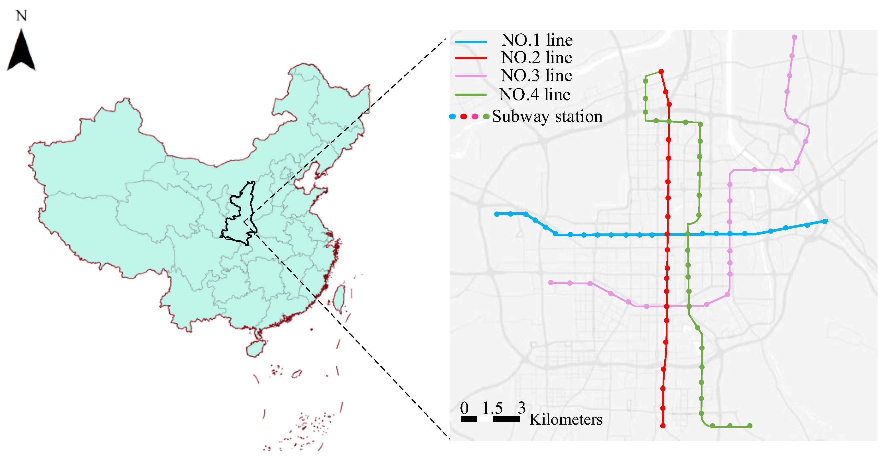
3.1. Research Area
3.2. Built Environment Variables
3.3. Smart Card Data
4. Methodology
4.1. XGBOOST Algorithm
4.2. SSA Algorithm
- Define the problem’s fitness function: Train the XGBOOST model based on the hyperparameter combinations and evaluate the model performance using methods such as cross-validation. Use the evaluation metrics as the value of the fitness function.
- Initialize the population: generate an initial set of hyperparameter combinations as the population.
- Iterative search: in each generation, evaluate the population based on the fitness function and select individuals with higher fitness.
- Generate new individuals: based on the selected individuals, use the operations of the Sea Cucumber Optimization Algorithm (such as foraging and predator avoidance) to generate new individuals.
- Update the population: update the population based on the newly generated individuals.
- Termination condition: stop the search when the predetermined number of iterations is reached or the stopping condition is met, and return the hyperparameter combination with the highest fitness.
4.3. SHAP Attribution Analysis
5. Results
5.1. Descriptive Analysis
5.2. Hyperparametric Results of SSA Method
5.3. Significance Contribution of Built Environment Factors
5.4. Comparison of Model Results
5.5. SHAP Summary Chart
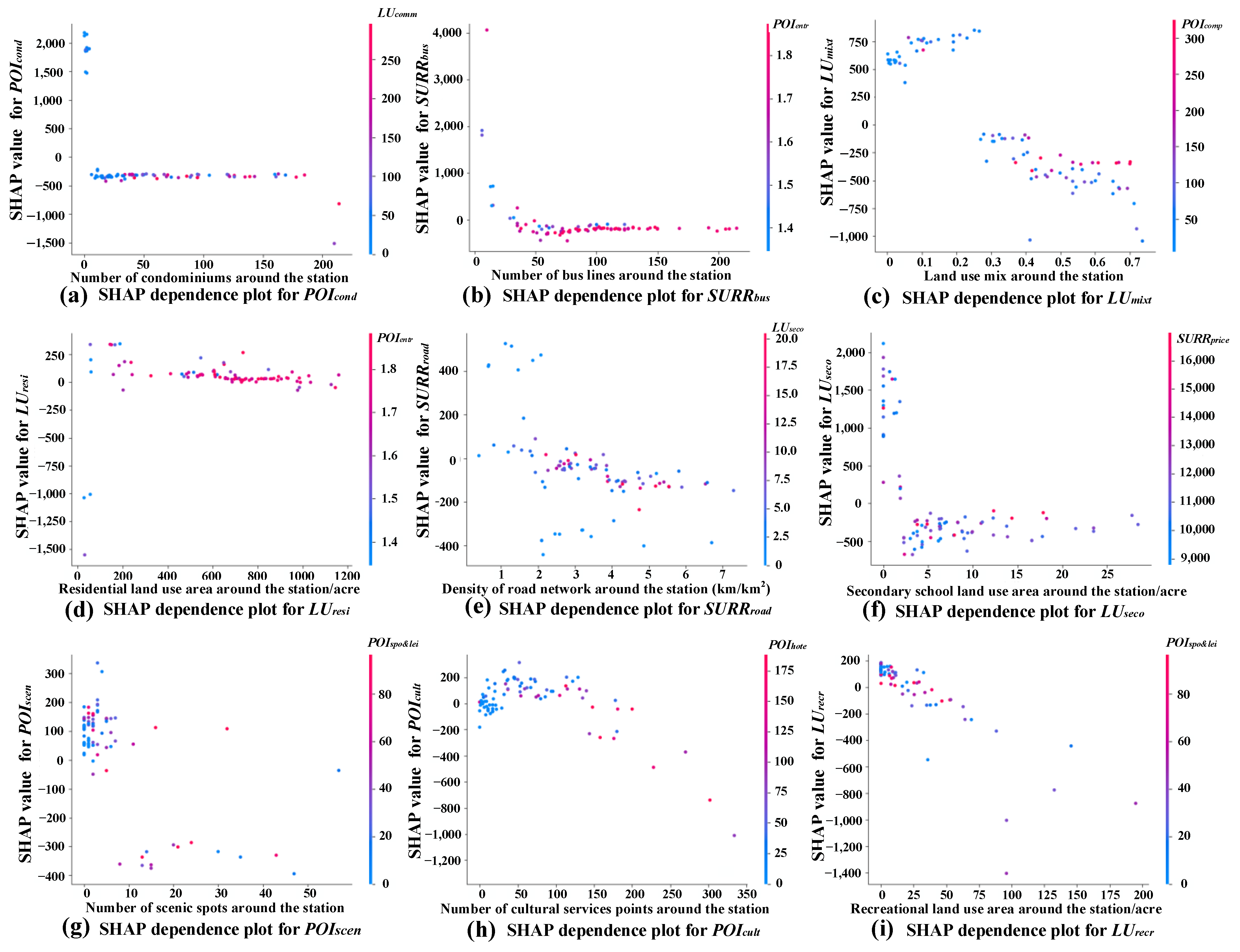
5.6. SHAP Partial Dependence
6. Discussion and Conclusions
6.1. Key Findings
6.2. Policy Implications
6.3. Limitations and Future Work
Author Contributions
Funding
Data Availability Statement
Acknowledgments
Conflicts of Interest
References
- Liu, L.; Wang, Y.; Hickman, R. How Rail Transit Makes a Difference in People’s Multimodal Travel Behaviours: An Analysis with the XGBoost Method. Land 2023, 12, 675. [Google Scholar] [CrossRef]
- Kwon, J.-H.; Cho, G.-H. The Long-Lasting Impact of Past Mobility Dependence on Travel Mode Share in a New Neighborhood: The Case of the Seoul Metropolitan Area, South Korea. Land 2023, 12, 1922. [Google Scholar] [CrossRef]
- Kim, M.; Cho, G.-H. Analysis on bike-share ridership for origin-destination pairs: Effects of public transit route characteristics and land-use patterns. J. Transp. Geogr. 2021, 93, 103047. [Google Scholar] [CrossRef]
- Yin, J.; Cao, X.J.; Huang, X. Association between subway and life satisfaction: Evidence from Xi’an, China. Transp. Res. Part D Transp. Environ. 2021, 96, 102869. [Google Scholar] [CrossRef]
- Gan, Z.; Yang, M.; Feng, T.; Timmermans, H.J. Examining the relationship between built environment and metro ridership at station-to-station level. Transp. Res. Part D Transp. Environ. 2020, 82, 102332. [Google Scholar] [CrossRef]
- Chen, E.; Ye, Z.; Bi, H. Incorporating smart card data in spatio-temporal analysis of metro travel distances. Sustainability 2019, 11, 7069. [Google Scholar] [CrossRef]
- Tao, T.; Cao, J. Exploring nonlinear and collective influences of regional and local built environment characteristics on travel distances by mode. J. Transp. Geogr. 2023, 109, 103599. [Google Scholar] [CrossRef]
- Peng, H.; Wen-xi, L.; Yan, L.; Qi, X. Spatial Patterns of Nonlinear Effects of Built Environment on Beijing Subway Ridership. J. Transp. Syst. Eng. Inf. Technol. 2023, 23, 187. [Google Scholar] [CrossRef]
- Wang, A.; Peng, J.; Ren, P.; Yang, H.; Dai, Q. Impact of the built environment of rail transit stations on the travel behavior of persons with disabilities: Taking 189 rail transit stations in Wuhan City as an example. Prog Geogr 2021, 40, 1127–1140. [Google Scholar] [CrossRef]
- Lin, Y.; Fu, H.; Zhong, Q.; Zuo, Z.; Chen, S.; He, Z.; Zhang, H. The influencing mechanism of the communities’ built environment on residents’ subjective well-being: A case study of Beijing. Land 2024, 13, 793. [Google Scholar] [CrossRef]
- Guo, H.; Bai, Y.; Hu, Q.; Zhuang, H.; Feng, X. Optimization on metro timetable considering train capacity and passenger demand from intercity railways. Smart Resilient Transp. 2021, 3, 66–77. [Google Scholar] [CrossRef]
- Shang, P.; Li, R.; Yang, L. Optimization of urban single-line metro timetable for total passenger travel time under dynamic passenger demand. Procedia Eng. 2016, 137, 151–160. [Google Scholar] [CrossRef]
- Ta, N.; Zhao, Y.; Chai, Y. Built environment, peak hours and route choice efficiency: An investigation of commuting efficiency using GPS data. J. Transp. Geogr. 2016, 57, 161–170. [Google Scholar] [CrossRef]
- Khan, M.; Kockelman, K.M.; Xiong, X. Models for anticipating non-motorized travel choices, and the role of the built environment. Transp. Policy 2014, 35, 117–126. [Google Scholar] [CrossRef]
- Guzman, L.A.; Peña, J.; Carrasco, J.A. Assessing the role of the built environment and sociodemographic characteristics on walking travel distances in Bogotá. J. Transp. Geogr. 2020, 88, 102844. [Google Scholar] [CrossRef]
- Long, Y.; Thill, J.-C. Combining smart card data and household travel survey to analyze jobs–housing relationships in Beijing. Computers, Environment and Urban Systems 2015, 53, 19–35. [Google Scholar] [CrossRef]
- Wang, Z.; Hu, Y.; Zhu, P.; Qin, Y.; Jia, L. Ring aggregation pattern of metro passenger trips: A study using smart card data. Phys. A Stat. Mech. Appl. 2018, 491, 471–479. [Google Scholar] [CrossRef]
- Gan, Z.; Feng, T.; Wu, Y.; Yang, M.; Timmermans, H. Station-based average travel distance and its relationship with urban form and land use: An analysis of smart card data in Nanjing City, China. Transp. Policy 2019, 79, 137–154. [Google Scholar] [CrossRef]
- Xu, X.-Y.; Kong, Q.-X.; Ji, J.-M.; Liu, J.; Sun, Q. Analysis of spatio-temporal heterogeneity impact of built environment on rail transit passenger flow. J. Transp. Syst. Eng. Inf. Technol. 2023, 23, 194. [Google Scholar] [CrossRef]
- Zhou, M.; Wang, D.; Guan, X. Co-evolution of the built environment and travel behaviour in Shenzhen, China. Transp. Res. Part D: Transp. Environ. 2022, 107, 103291. [Google Scholar] [CrossRef]
- Chang, T.; Yang, D.; Yang, Y.; Huo, J.; Wang, G.; Xiong, C. Impact of urban rail transit on business districts based on time distance: Urumqi Light Rail. J. Urban Plan. Dev. 2018, 144, 04018024. [Google Scholar] [CrossRef]
- Chen, F.; Wu, J.; Chen, X.; Wang, J. Vehicle kilometers traveled reduction impacts of transit-oriented development: Evidence from Shanghai City. Transp. Res. Part D Transp. Environ. 2017, 55, 227–245. [Google Scholar] [CrossRef]
- Choi, K. The influence of the built environment on household vehicle travel by the urban typology in Calgary, Canada. Cities 2018, 75, 101–110. [Google Scholar] [CrossRef]
- Kim, J.; Brownstone, D. The impact of residential density on vehicle usage and fuel consumption: Evidence from national samples. Energy Econ. 2013, 40, 196–206. [Google Scholar] [CrossRef]
- Zhang, L.; Hong, J.; Nasri, A.; Shen, Q. How built environment affects travel behavior: A comparative analysis of the connections between land use and vehicle miles traveled in US cities. J. Transp. Land Use 2012, 5, 40–52. [Google Scholar] [CrossRef]
- Choi, J.; Lee, Y.J.; Kim, T.; Sohn, K. An analysis of Metro ridership at the station-to-station level in Seoul. Transportation 2012, 39, 705–722. [Google Scholar] [CrossRef]
- Iseki, H.; Liu, C.; Knaap, G. The determinants of travel demand between rail stations: A direct transit demand model using multilevel analysis for the Washington DC Metrorail system. Transp. Res. Part A Policy Pract. 2018, 116, 635–649. [Google Scholar] [CrossRef]
- Eliasson, J. Will we travel less after the pandemic? Transp. Res. Interdiscip. Perspect. 2022, 13, 100509. [Google Scholar] [CrossRef]
- Wang, X.; Pei, T.; Li, K.; Cen, Y.; Shi, M.; Zhuo, X.; Mao, T. Analysis of changes in population’s cross-city travel patterns in the pre-and post-pandemic era: A case study of China. Cities 2022, 122, 103472. [Google Scholar] [CrossRef]
- Liu, J.; Cao, Q.; Pei, M. Impact of COVID-19 on adolescent travel behavior. J. Transp. Health 2022, 24, 101326. [Google Scholar] [CrossRef]
- Chen, K.; Steiner, R. Longitudinal and spatial analysis of Americans’ travel distances following COVID-19. Transp. Res. Part D Transp. Environ. 2022, 110, 103414. [Google Scholar] [CrossRef]
- An, D.; Tong, X.; Liu, K.; Chan, E.H. Understanding the impact of built environment on metro ridership using open source in Shanghai. Cities 2019, 93, 177–187. [Google Scholar] [CrossRef]
- Caset, F.; Blainey, S.; Derudder, B.; Boussauw, K.; Witlox, F. Integrating node-place and trip end models to explore drivers of rail ridership in Flanders, Belgium. J. Transp. Geogr. 2020, 87, 102796. [Google Scholar] [CrossRef]
- Chen, E.; Ye, Z.; Wang, C.; Zhang, W. Discovering the spatio-temporal impacts of built environment on metro ridership using smart card data. Cities 2019, 95, 102359. [Google Scholar] [CrossRef]
- Liu, M.; Liu, Y.; Ye, Y. Nonlinear effects of built environment features on metro ridership: An integrated exploration with machine learning considering spatial heterogeneity. Sustain. Cities Soc. 2023, 95, 104613. [Google Scholar] [CrossRef]
- Chen, E.; Ye, Z.; Wu, H. Nonlinear effects of built environment on intermodal transit trips considering spatial heterogeneity. Transp. Res. Part D Transp. Environ. 2021, 90, 102677. [Google Scholar] [CrossRef]
- Su, S.; Wang, Z.; Li, B.; Kang, M. Deciphering the influence of TOD on metro ridership: An integrated approach of extended node-place model and interpretable machine learning with planning implications. J. Transp. Geogr. 2022, 104, 103455. [Google Scholar] [CrossRef]
- Yan, X.; Liu, X.; Zhao, X. Using machine learning for direct demand modeling of ridesourcing services in Chicago. J. Transp. Geogr. 2020, 83, 102661. [Google Scholar] [CrossRef]
- Teixeira, J.F.; Lopes, M. The link between bike sharing and subway use during the COVID-19 pandemic: The case-study of New York’s Citi Bike. Transp. Res. Interdiscip. Perspect. 2020, 6, 100166. [Google Scholar] [CrossRef]
- Yu, L.; Cong, Y.; Chen, K. Determination of the peak hour ridership of metro stations in Xi’an, China using geographically-weighted regression. Sustainability 2020, 12, 2255. [Google Scholar] [CrossRef]
- De Gruyter, C.; Butt, A.; Davies, L. Exploring the potential for unbundling off-street car parking in residential apartment buildings. Transport Policy 2024. [CrossRef]
- Yang, L.; Yu, B.; Liang, Y.; Lu, Y.; Li, W. Time-varying and non-linear associations between metro ridership and the built environment. Tunn. Undergr. Space Technol. 2023, 132, 104931. [Google Scholar] [CrossRef]
- Yang, H.; Zhao, Z.; Jiang, C.; Wen, Y.; Muneeb Abid, M. Spatially Varying Relation between Built Environment and Station-Level Subway Passenger-Distance. J. Adv. Transp. 2022, 2022, 7542560. [Google Scholar] [CrossRef]
- Zhao, J.; Deng, W.; Song, Y.; Zhu, Y. What influences Metro station ridership in China? Insights from Nanjing. Cities 2013, 35, 114–124. [Google Scholar] [CrossRef]
- Sohn, K.; Shim, H. Factors generating boardings at Metro stations in the Seoul metropolitan area. Cities 2010, 27, 358–368. [Google Scholar] [CrossRef]


| Variable | Description | Mean | STD | Unit |
|---|---|---|---|---|
| LUcomm | Area of commercial land around station | 120.018 | 107.658 | Acre |
| LUrecr | Area of recreational land around station | 19.805 | 35.065 | Acre |
| LUresi | Area of residential land around station | 626.096 | 288.492 | Acre |
| LUwork | Area of working land around station | 61.441 | 56.512 | Acre |
| LUseco | Area of secondary school land around station | 6.634 | 6.508 | Acre |
| LUuniv | Area of university land around station | 14.640 | 29.219 | Acre |
| LUmixt | Degree of land use mix around station | 0.343 | 0.232 | |
| POIcond | Number of condominiums around station | 56.287 | 55.451 | |
| POIspo&lei | Number of sports and leisure centers around station | 32.333 | 33.693 | |
| POIscen | Number of scenic spots around station | 6.345 | 10.959 | |
| POIcult | Number of cultural services around station | 69.459 | 76.169 | |
| POIhote | Number of hotel residences around station | 51.414 | 61.134 | |
| POIshop | Number of shopping points around station | 8.667 | 8.537 | |
| POIcate | Number of catering services around station | 179.655 | 154.154 | |
| POIcomp | Number of companies around station | 103.436 | 132.414 | |
| SURRroad | Density of road network around station | 3.368 | 1.504 | km/km2 |
| SURRbus | Number of bus lines around station | 89.977 | 47.165 | |
| SURRprice | House prices around station | 11,149.7 | 2697.441 | CNY |
| SURRhous | Number of houses around station | 12,720.334 | 11,057.133 | |
| STATdist | Distance from station to city center | 7.494 | 4.035 | km |
| ID | Swipe Time | Type of Entry/Exit Station | Line | Station |
|---|---|---|---|---|
| 1F022702 | 20201123062152 | 1 | 2 | 9860 |
| 1F022711 | 20201123062217 | 1 | 3 | 1600 |
| 1F024108 | 20201123083509 | 2 | 1 | 3300 |
| 1F02531A | 20171123062105 | 2 | 3 | 258 |
| Hyperparameterization | Explanation | Range of Values | Preferred Value |
|---|---|---|---|
| max_depth | Maximum depth of the tree | [1, 10] | 4 |
| learning_rate | Learning rate | [0.01, 0.1] | 0.09 |
| subsample | Subsampling rate | [0.5, 0.9] | 0.75 |
| colsample_bytree | Column sampling rate | [0.5, 0.9] | 0.62 |
| n_estimators | Number of regression trees | [100, 200] | 154 |
| Gamma | Leaf node splitting threshold | [0, 5] | 0 |
| Morning Peak | Evening Peak | ||||
|---|---|---|---|---|---|
| Variable | Relative Importance (%) | Ranking | Variable | Relative Importance (%) | Ranking |
| STATdist | 43.210 | 1 | STATdist | 66.339 | 1 |
| POIcond | 27.997 | 2 | SURRroad | 10.259 | 2 |
| SURRbus | 6.215 | 3 | SURRbus | 6.191 | 3 |
| LUmixt | 5.349 | 4 | SURRhous | 6.134 | 4 |
| LUresi | 3.996 | 5 | LUmixt | 2.779 | 5 |
| SURRroad | 3.843 | 6 | LUrecr | 1.516 | 6 |
| LUseco | 2.009 | 7 | POIcult | 1.159 | 7 |
| POIscen | 1.463 | 8 | LUresi | 1.057 | 8 |
| POIcult | 1.099 | 9 | LUseco | 0.983 | 9 |
| LUrecr | 1.011 | 10 | POIcomp | 0.901 | 10 |
| Peak Period | Model | R-Squared | MAE | RMSE |
|---|---|---|---|---|
| Morning peak | SSA-XGBOOST | 0.633 | 1114.660 | 1420.421 |
| XGBOOST | 0.611 | 1145.251 | 1468.254 | |
| GBDT | 0.577 | 1215.802 | 1515.450 | |
| OLS | 0.415 | 1315.454 | 1592.725 | |
| Evening peak | SSA-XGBOOST | 0.583 | 1277.125 | 1572.279 |
| XGBOOST | 0.544 | 1312.252 | 1624.201 | |
| GBDT | 0.511 | 1342.251 | 1671.007 | |
| OLS | 0.408 | 1411.052 | 1715.445 |
Disclaimer/Publisher’s Note: The statements, opinions and data contained in all publications are solely those of the individual author(s) and contributor(s) and not of MDPI and/or the editor(s). MDPI and/or the editor(s) disclaim responsibility for any injury to people or property resulting from any ideas, methods, instructions or products referred to in the content. |
© 2024 by the authors. Licensee MDPI, Basel, Switzerland. This article is an open access article distributed under the terms and conditions of the Creative Commons Attribution (CC BY) license (https://creativecommons.org/licenses/by/4.0/).
Share and Cite
Li, P.; Yang, Q.; Lu, W. Nonlinear Relationship of Multi-Source Land Use Features with Temporal Travel Distances at Subway Station Level: Empirical Study from Xi’an City. Land 2024, 13, 1021. https://doi.org/10.3390/land13071021
Li P, Yang Q, Lu W. Nonlinear Relationship of Multi-Source Land Use Features with Temporal Travel Distances at Subway Station Level: Empirical Study from Xi’an City. Land. 2024; 13(7):1021. https://doi.org/10.3390/land13071021
Chicago/Turabian StyleLi, Peikun, Quantao Yang, and Wenbo Lu. 2024. "Nonlinear Relationship of Multi-Source Land Use Features with Temporal Travel Distances at Subway Station Level: Empirical Study from Xi’an City" Land 13, no. 7: 1021. https://doi.org/10.3390/land13071021