Spatial Distribution of the Cropping Pattern Exerts Greater Influence on the Water Footprint Compared to Diversification in Intensive Farmland Landscapes

Abstract

Global imperatives call for reduced water consumption in homogeneous, intensive farming systems, where farmland landscape heterogeneity significantly impacts anthropogenic, ecological, and socioeconomic factors. However, the impact of this heterogeneity on crop water footprint (WF) remains uncertain. To address this, this study assessed the WF at the landscape scale across 616 subplots (1 × 1 km) in a representative county of North China Plain from 2013 to 2019, integrating green (WF_green), blue (WF_blue), and gray (WF_gray) water footprints. Results showed that the winter wheat–summer maize double cropping pattern (WM) exhibited the highest WF_green, WF_blue, and WF_gray. Over six years, most subplots saw significant reductions in WF_green, WF_blue, WF_gray, and WF. At the landscape scale, diversification (compositional heterogeneity), fragmentation, and spatial distribution (configurational heterogeneity) were assessed using Shannon’s diversity index (SHDI), edge density (ED), and effective mesh size (MESH), which exhibited average variations of 0.07, −3.16 m ha⁻¹, and −5.86 m², respectively. For WM patches, the percentage of landscape (PLAND) and MESH were used to evaluate diversification and spatial distribution, resulting in reductions of 1.14% and 2.32 m², respectively. Regression analysis and structural equation modeling further illuminated the connections between the landscape pattern and WF, emphasizing the significant role of MESH in reducing WF_blue and influencing crop diversity (p < 0.001). Therefore, spatial distribution, whether directly or through the mediation of diversification, demonstrated a more substantial overall impact on WF. Consequently, future research should prioritize investigating how spatial distribution influences crop choice and agronomic management in order to determine the optimal cropping patterns and field size that strike a balance between crop production and the water footprint. This study offers theoretical guidance and a scientific foundation for redesigning farmland landscapes to bolster water sustainability in intensive farming systems.

1. Introduction

To meet the escalating global demand for food under resource constraints, intensive farming has garnered widespread adoption on a global scale [1,2,3]. Characterized by vast fields and homogeneous farmland landscapes, intensive farming systems heavily depend on external inputs. These inputs impose a severe threat to the well-being of aquatic, terrestrial, and atmospheric ecosystems, leading to substantial concerns regarding pollution [4,5,6]. Extensive research has conclusively demonstrated the positive impacts of diversified cropping methods, encompassing multiple cropping, crop rotation, intercropping and relay cropping, and agroforestry, on both crop yield and the provision of ecosystem services [7,8,9,10,11]. Nevertheless, scant attention has been given to investigating the ramifications of shifting landscape heterogeneity on water sustainability within the context of farmland landscape redesigning.

Farmland landscape heterogeneity comprises compositional heterogeneity and configurational heterogeneity, which, respectively, describe the diversification of the land cover type and its spatial distribution. It is governed by the direct and indirect influences of crops and non-crops on ecological processes, the farmland landscape structure, and ecosystem services [12,13,14]. Landscape pattern metrics are indispensable tools for assessing landscape heterogeneity. These metrics quantify farmland landscape heterogeneity at the patch, class, and landscape scales to comprehensively illustrate the effects of agronomic practices, geographical processes, natural resources, and socioeconomic development [15,16,17]. Landscape pattern metrics have historically been used to quantify relevant impacts of landscape heterogeneity triggered by ecosystem changes, with specific emphases on yield, pollination, and pest management resulting from adjustments in crop and non-crop diversity and abundance [7,8,9,11]. Under intensive crop production conditions, farmland landscape yield increases as the area of continuous single-crop fields expands, leading to reduced landscape heterogeneity and its reduced long-term sustainability [18,19,20,21]. Thus, planning and redesigning sustainable landscape patterns are essential for safeguarding the stability and security of the farmland landscape [22,23]. Agronomic practices, as the dominant human activity shaping the local farmland landscape heterogeneity, possess substantial potential to boost crop yield without degrading the environment [24,25]. However, limited attention has been directed towards examining the influence of agronomic practices on the farmland landscape heterogeneity, particularly within intensive farming systems. Consequently, studying the characteristics of spatiotemporal variations in farmland landscape heterogeneity serves as a fundamental cornerstone for enhancing landscape sustainability.

Water resources pose a significant constraint on food production and represent one of the fundamental challenges in meeting the demands of a growing global population [26]. Water footprint has been proposed as a comprehensive indicator to provide insights into human impact on water resources by quantifying water consumption [27]. Crop water footprint (WF) consists of three components: green water footprint (WF_green), blue water footprint (WF_blue), and gray water footprint (WF_gray). It evaluates the exploitation of regional water resources by assessing the direct and indirect water consumptions associated with crop production throughout the growing period [28,29]. Specifically, WF_green represents crop evapotranspiration from effective rainfall, whereas WF_blue accounts for crop evapotranspiration from surface and underground water through irrigation. WF_gray refers to the water requirement to assimilate pollutants from external inputs to acceptable concentrations according to water quality standards [30]. The overarching objective of the WF is to enhance water resource sustainability by reducing water consumption and improving water use efficiency [31,32]. Various factors, including crop types, cropping systems, climatic conditions, irrigation methods, and external inputs, can influence WF, making its precise evaluation and forecasting challenging [27,33]. Previous studies have primarily focused on calculating the WF at the field, regional, or global scale to compare water consumption, estimate water scarcity, and explore strategies for improving water sustainability through irrigation management and changing cropping patterns [27,34,35,36,37]. Additionally, quantitative research has employed WF_gray to measure water pollution and to assess the environmental impacts of crop production [38,39,40]. Furthermore, based on the spatiotemporal distribution of limited grain crops, such as rice, wheat, and maize, few studies have examined the effects of landscape heterogeneity on water sustainability in the North China Plain [15].

To fill this research gap, we quantified the spatiotemporal variations in the farmland landscape heterogeneity and the WF of major crops and cropping patterns within 1 × 1 km subplots in a representative county. The objectives of this study were: (1) to quantify the WFs of major crops and cropping patterns; (2) to examine variations in the farmland landscape heterogeneity and the WF at the landscape scale and in WM patches; and (3) ultimately, to investigate the influences of farmland landscape heterogeneity on the WF. This study would offer a new perspective to enhance water sustainability through optimizing crop choice and field size in farmland landscape redesigning.

2. Materials and Methods

2.1. Study Area

Wuqiao County (37°41′ N, 116°37′ E) was selected as the study area (Figure S1), with 68% of its land classified as arable [41]. The selection of this representative county was motivated by several factors. Firstly, Wuqiao represents a typical case of intensive farming practices within the North China Plain, exhibiting characteristic cropping patterns, farmland crop diversity, soil properties, climate conditions, agricultural policies, and resource scarcity [42,43,44]. Secondly, the selection of the county scale allows for a focused investigation into the spatiotemporal variations in landscape heterogeneity resulting from crop variations, rather than factors such as policy, soil properties, topography, and climate. Lastly, images with high spatial resolution and comprehensive cropping pattern information, which are essential for heterogeneity analysis, are available to be interpreted at the county level.

The annual average temperature of Wuqiao was 12.6 °C, the total effective accumulative temperature was 4665 °C, and the total annual average precipitation was 530 mm (mostly from June to August). The per capita available water resource was 190 m³, significantly lower than the threshold for extreme water scarcity [45]. Since 2012, crop composition and distribution have changed. Wheat, maize, cotton, pepper, and peanut, which are major crops in the North China Plain, accounted for approximately 90% of Wuqiao’s planting area [46].

2.2. Basic Data

The basic data encompassed various key aspects, including meteorological data, spatiotemporal crop distribution, external inputs during crop production, and soil information. To obtain comprehensive meteorological records spanning the period from 1990 to 2020, daily observed maximum and minimum temperatures, average temperature, relative humidity, precipitation, wind speed, and sunshine duration were obtained from the Wuqiao meteorological station, one of China’s national surface meteorological stations. Given the sensitivity of farmland landscape heterogeneity to small-area crops, we made efforts to accurately represent the actual farmland landscape by interpreting 7 cropping patterns. These cropping patterns were the winter wheat–summer maize double cropping pattern (WM), the cotton single cropping pattern (COTTONTTON), pepper single cropping pattern (PEPPER), spring maize single cropping pattern (MAIZE), peanut single cropping pattern (PEANUT), tree crop single cropping pattern (TCS), and tree crop double cropping pattern (TCD). The cropping patterns were interpreted based on the land-use map, Landsat 8, and Sentinel 2 images in 2013 and 2019, which were previously published [47]. External inputs for crop production, such as fertilizer, pesticide, and irrigation, were gathered by investigation.

2.3. Spatial Sampling

According to previous studies [48,49], a fishnet was employed in ArcGIS10.6 to establish 1 × 1 km subplots to process the WF and landscape pattern metrics in the study area (Figure S1). To ensure a comprehensive evaluation of landscape metrics and the WF while minimizing potential human biases, a total of 616 subplots were ultimately selected.

2.4. Calculation of Water Footprint

The WF was undertaken to assess the impacts of human activities on water resources to reduce water consumption and enhance water sustainability. In this study, WF analysis was performed on the basis of the water footprint network. The WFs for several crops were independently calculated as follows:

$$\mathrm{W}\mathrm{F}={\mathrm{W}\mathrm{F}}_{\mathrm{g}\mathrm{r}\mathrm{e}\mathrm{e}\mathrm{n}}+{\mathrm{W}\mathrm{F}}_{\mathrm{b}\mathrm{l}\mathrm{u}\mathrm{e}}+{\mathrm{W}\mathrm{F}}_{\mathrm{g}\mathrm{r}\mathrm{a}\mathrm{y}}$$

(1)

The USDA-SCS method and Penman–Monteith model were used to evaluate WF_green, which is related to effective rainfall in crop production [50]. The calculation is shown below:

$${\mathrm{W}\mathrm{F}}_{\mathrm{g}\mathrm{r}\mathrm{e}\mathrm{e}\mathrm{n}}=10\times {\sum }_{d=1}^{lgp}{ET}_{green}$$

(2)

$${ET}_{green}=Min(P_{eff}, {ET}_c)$$

(3)

$$P_{eff}=\left\{\begin{array}{c}P\times (41.7-0.2\times P)/41.7 P\le 83 \mathrm{mm}\\ 41.7+0.1P P>83 \mathrm{mm}\end{array}\right.$$

(4)

$${ET}_c={ET}_0\times K_c$$

(5)

$${ET}_0=\frac{0.408∆(R_n-G)+\frac{900\gamma U_2(e_a-e_d)}{T+273}}{∆+\gamma (1+0.34U_2)}$$

(6)

where ET_green is the evapotranspiration of green water (mm day⁻¹); lgp refers to the growing season length; P_eff represents effective rainfall (mm day⁻¹); P represents precipitation (mm day⁻¹); ET_c is the evapotranspiration of different crops (mm day⁻¹); ET₀ is the reference crop evapotranspiration (mm day⁻¹); and K_c is the crop coefficient, which is related to the growing period and the crop type. The K_c for each crop was mainly obtained from the Food and Agriculture Organization of the United Nations (FAO) [50]. R_n is the net radiation on the crop surface (MJ m⁻²day⁻¹); G is the soil heat flux density (MJ m⁻²day⁻¹); γ is the psychrometric constant (kPa °C⁻¹); U₂ represents the wind speed at 2 m (m s⁻¹); e_a is the saturation vapor pressure (kPa); e_d is the actual vapor pressure (kPa); T is the air temperature at 2 m (°C); and Δ represents the slope of the vapor pressure curve (kPa °C⁻¹).

$${\mathrm{W}\mathrm{F}}_{\mathrm{b}\mathrm{l}\mathrm{u}\mathrm{e}}=10\times {\sum }_{d=1}^{lgp}{ET}_{blue}$$

(7)

$${ET}_{blue}=max(0,{ET}_a-P_{eff})$$

(8)

where ET_blue represents the evapotranspiration of blue water (mm day⁻¹); ET_a is the actual evapotranspiration of different crops, which is obtained by the CROPWAT model (mm).

$${\mathrm{W}\mathrm{F}}_{\mathrm{g}\mathrm{r}\mathrm{a}\mathrm{y}}=\frac{\alpha \times AR}{c_{max}-c_{nat}}$$

(9)

where α is the leaching rate; AR represents the external inputs that act as pollutants (kg ha⁻¹); c_max represents the maximum allowable concentration of each external input (kg m⁻³); and c_nat is the natural concentration of each pollutant. The leaching rate of external inputs on farmland was obtained from national investigations based on typical cropping patterns and representative land-use types in China’s major planting zone [51].

2.5. Calculation of Landscape Heterogeneity

Considering that landscape heterogeneity is greatly influenced by patch characteristics [52], a set of landscape pattern metrics at the landscape and patch scales through subplots was investigated [53,54,55,56]. The metrics can reflect compositional and configurational heterogeneity, as well as fragmentation.

Specifically, seven metrics at the landscape scale were chosen to describe heterogeneity (Table S1). Effective mesh size (MESH), splitting index (SPLIT), and landscape division index (DIVISION) were selected to describe spatial distribution. Shannon’s diversity index (SHDI) and largest patch index (LPI) were employed to depict diversification. Moreover, edge density (ED) and the landscape shape index (LSI) were utilized to reveal fragmentation.

Furthermore, seven metrics were selected to characterize the heterogeneity of patches (Table S1). For spatial distribution, MESH, SPLIT, and DIVISION were employed. Meanwhile, percentage of landscape (PLAND) and LPI were chosen to describe diversification. Number of patches (NP) and LSI were used to reveal fragmentation.

2.6. Influences of Landscape Heterogeneity on Water Footprint

Given the non-normal distribution of the data, the Spearman correlation was initially employed to elucidate the relationships between landscape heterogeneity and WF. The correlation coefficient r was calculated as:

$$r=1-\frac{6\sum {\left(rg\right(l_i)-rg(w_i\left)\right)}^2}{n(n^2-1)}$$

(10)

where l and w represent landscape metrics and the WF of the subplots; n represents the number of subplots; and rg represents the serial number of reordering. The value of r indicates the strength of the relationships between landscape metrics and WF. Strong correlations were observed when the absolute value of r fell within the range of 0.5 to 1.0. Moderate correlations were observed within the range of 0.3 to 0.5. Weak correlations were observed within the range of 0.1 to 0.3. No correlation was observed within the range of 0 to 0.1. Landscape metrics that had a high r with the WF would be regarded as the recommended indicators for portraying landscape heterogeneity.

In order to characterize the influence of landscape heterogeneity on the WF, linear regression was employed on the differences in landscape metrics and the WF as:

$$∆w=a∆l+b$$

(11)

where coefficient a represents the influence of landscape heterogeneity changes on the WF when it passed the significance test.

2.7. Statistics and Mapping

Fragstats 4.2 was employed to calculate landscape metrics. Spatial maps were generated using ArcGIS 10.6. The Spearman correlation and linear regression analysis were performed using scipy and statsmodels packages with Python 3.7.4. Furthermore, structural equation modeling (SEM) was conducted through AMOS version 26.

3. Results

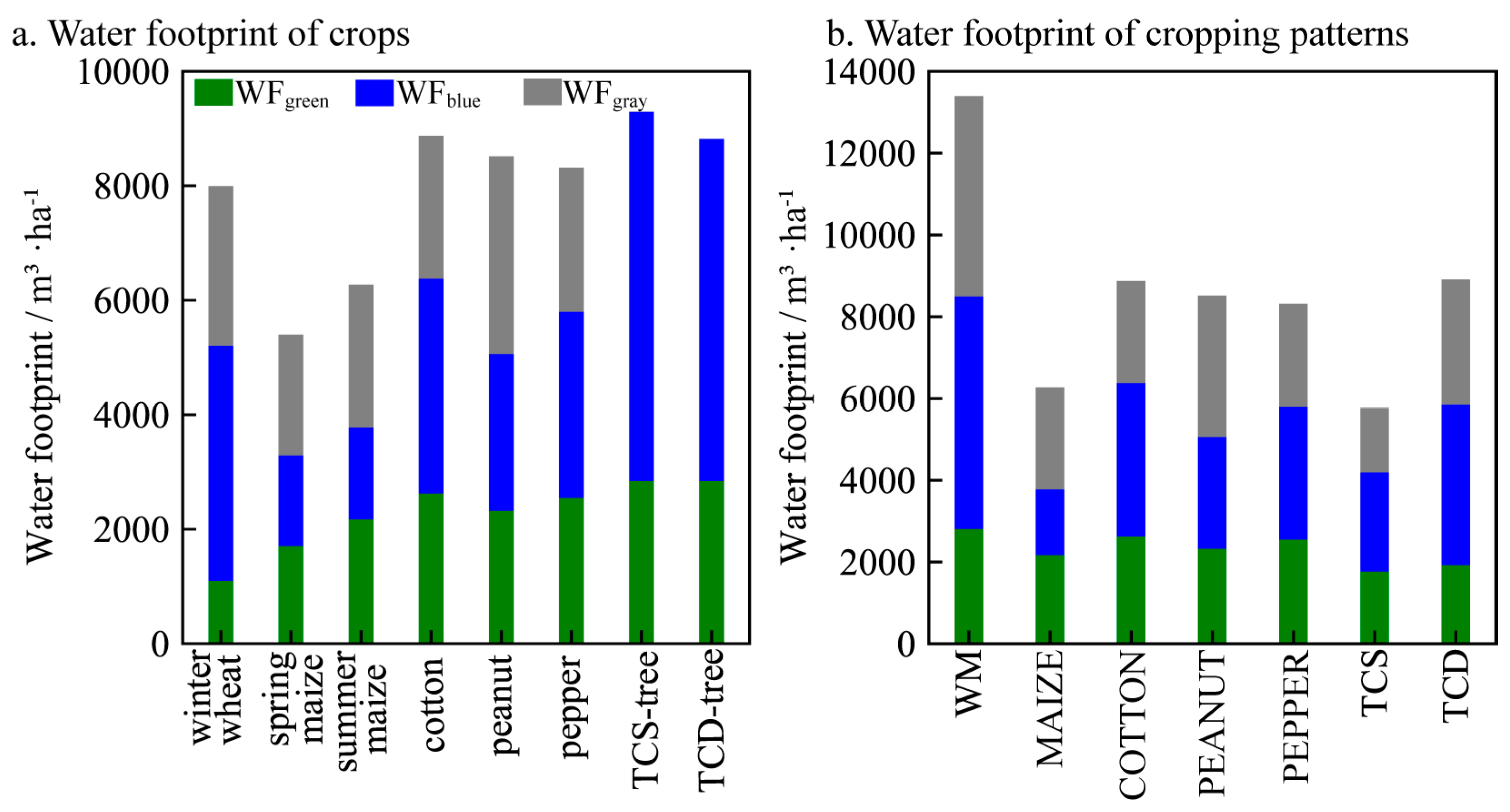
3.1. Water Footprints of Crops and Cropping Patterns

TCS-tree exhibited the highest WF, whereas summer maize had the lowest during the single growing season (Figure 1a). TCS-tree and TCD-tree had the highest WF_green at 2842 m³ ha⁻¹, whereas winter wheat exhibited the lowest at 1099 m³ ha⁻¹, owing to its shorter growth period during the rainy season. In addition, TCS-tree had the highest WF_blue at 6448 m³ ha⁻¹, while summer maize had the lowest at 1580 m³ ha⁻¹. Peanut demonstrated the highest WF_gray, while TCS-tree and TCD-tree had the lowest.

WM was the cropping pattern with the highest WF, whereas TCS had the lowest throughout the annual growing season (Figure 1b). WM recorded the highest values for WF_green, WF_blue, and WF_gray, reaching 2809 m³ ha⁻¹, 5691 m³ ha⁻¹, and 4893 m³ ha⁻¹, respectively, attributable to its substantial external inputs and long growth period.

3.2. Variations in Water Footprint and Landscape Heterogeneity

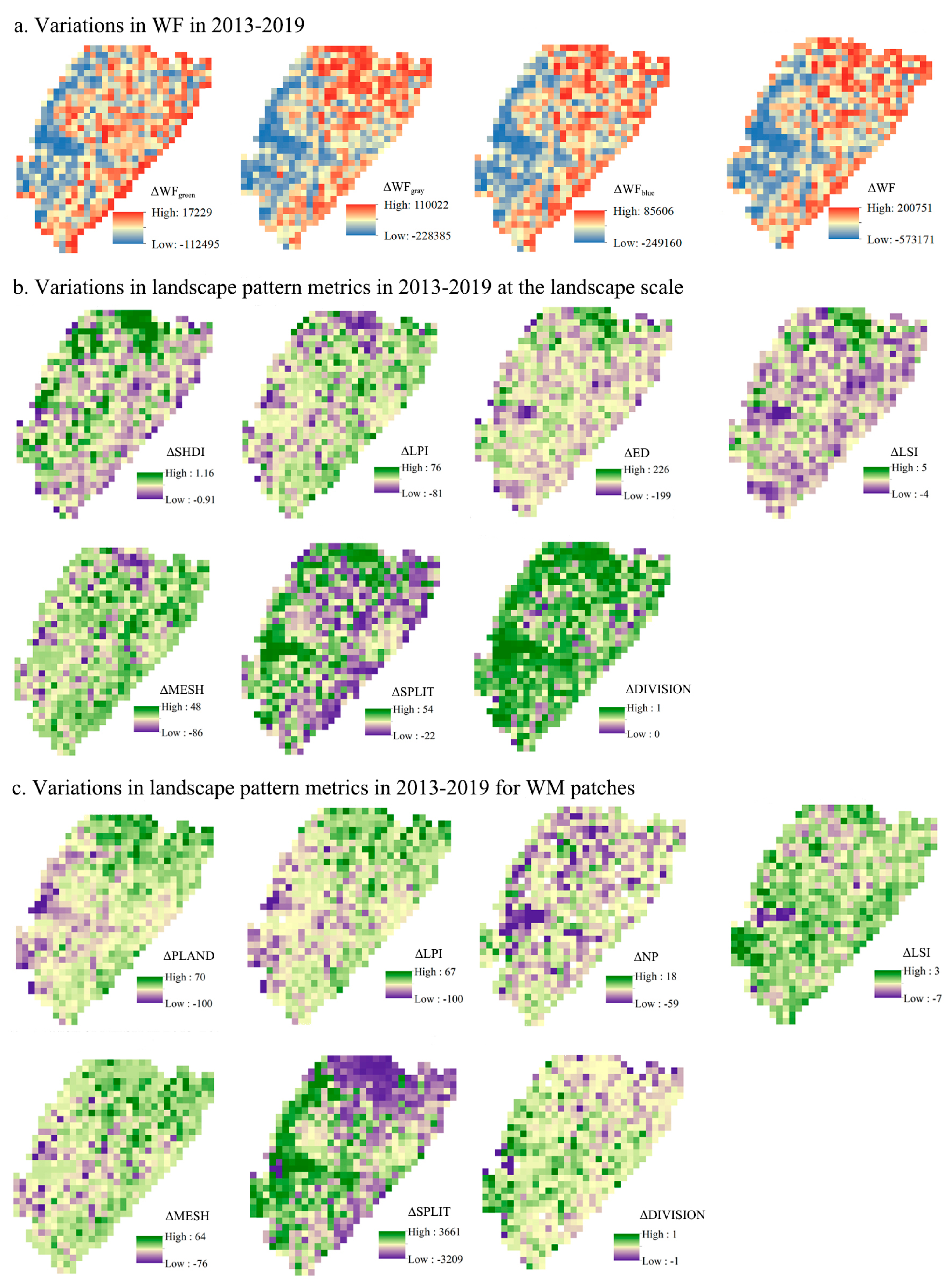
3.2.1. Variations in Water Footprint

Totals of 19.21% and 34.01% of the subplots experienced an increase in WF_green and WF_gray, respectively, with the majority concentrated in the eastern and northern regions (Figure 2a and Figure S2). However, 80.79% and 65.99% of the subplots exhibited a decrease in WF_green and WF_gray, respectively, dispersed across the study area. Additionally, 7.13% and 21.12% of the subplots demonstrated an increase in WF_blue and WF, respectively. Nevertheless, 92.87% and 78.88% of the subplots experienced a decline in WF_blue and WF.

3.2.2. Variations in Landscape Metrics at the Landscape Scale and in WM Patches

At the landscape scale, the average variation in SHDI was 0.07, and 55% of the subplots exhibited an increase (Figure 2b and Figure S3). The spatial allocations of and variations in LSI and ED at the landscape scale were comparable (Figure 2b and Figure S4). On average, ED and LSI showed decreases of −3.16 and −0.04, respectively, with 55% of the subplots experiencing a decrease. This indicated that the shape of the patches became more regular and less fragmented. The average variations in MESH and SPLIT were −5.86 and 1.92, respectively, with 62% of the subplots showing a decrease in MESH and an increase in SPLIT (Figure 2b and Figure S5). These results indicated that the majority of the subplots displayed a more complex spatial distribution.

Regarding WM patches, the average variation in NP was −7.20, with 83% of the subplots exhibiting a decrease, suggesting a significant reduction in fragmentation (Figure 2c and Figure S4). The average variation in MESH decreased by 2.32, with 55% of subplots experiencing a decrease (Figure 2c and Figure S5). Despite a 53% increase, the average variation in SPLIT was −28.67.

3.3. Influences of Landscape Heterogeneity on Water Footprint

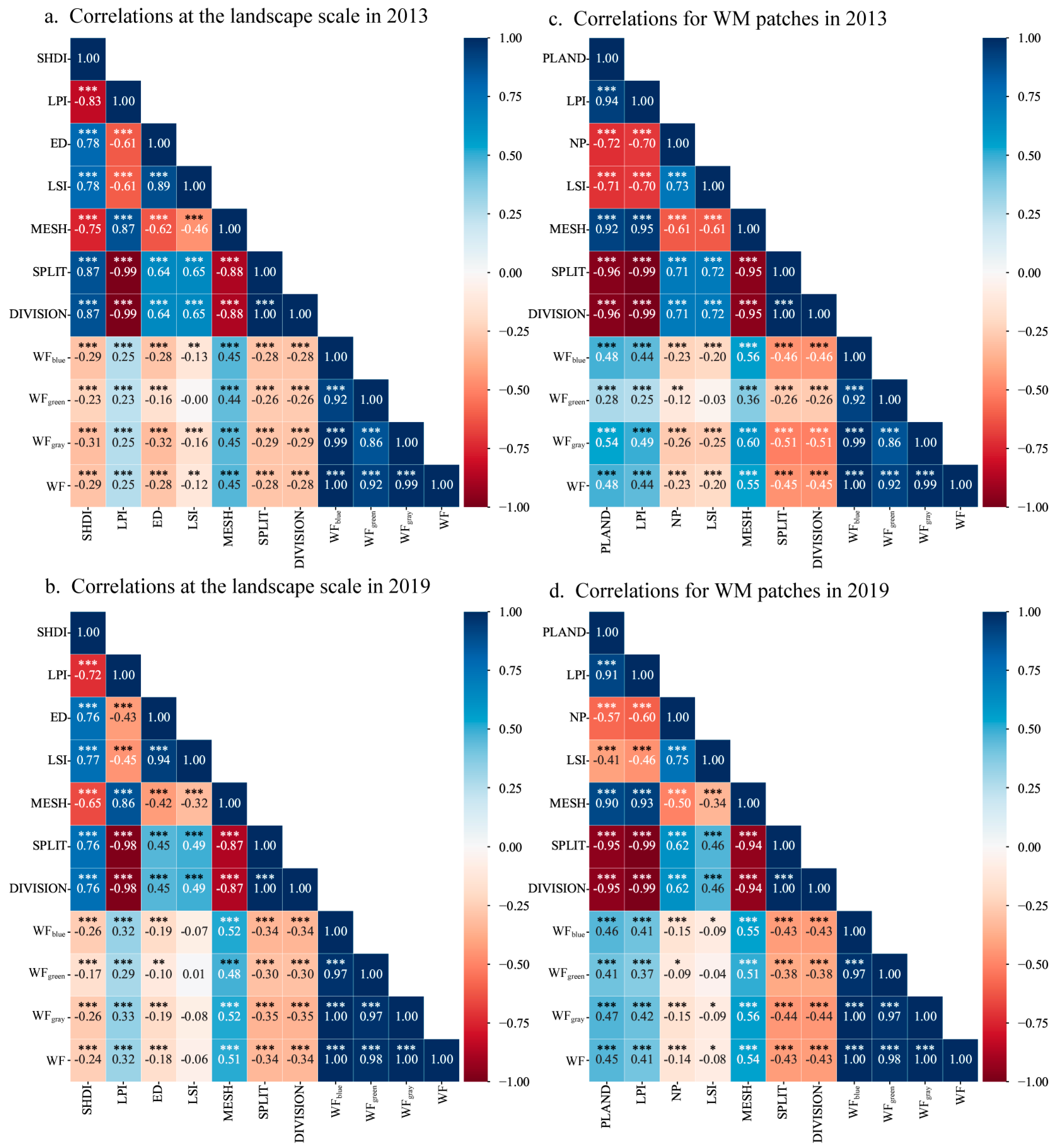
3.3.1. Correlations between Water Footprint and Landscape Metrics at the Landscape Scale and in WM Patches

At the landscape scale, the correlation analysis revealed that MESH exhibited a significant strong relationship with the WF, with coefficients falling around 0.5 (Figure 3). Conversely, LSI exhibited a weaker correlation than ED. Furthermore, SHDI demonstrated a stronger correlation with the WF, compared to LPI. Landscape heterogeneity was found to be negatively associated with the WF.

For WM patches, the landscape pattern metrics were found to have a stronger correlation with the WF (Figure 3). Spatial distribution showed a strong correlation with WF, with the coefficients being higher than 0.5. Diversification showed a moderate correlation, with the coefficients falling around 0.45. Moreover, the WF was detected to have a negative correlation with the heterogeneity of WM patches.

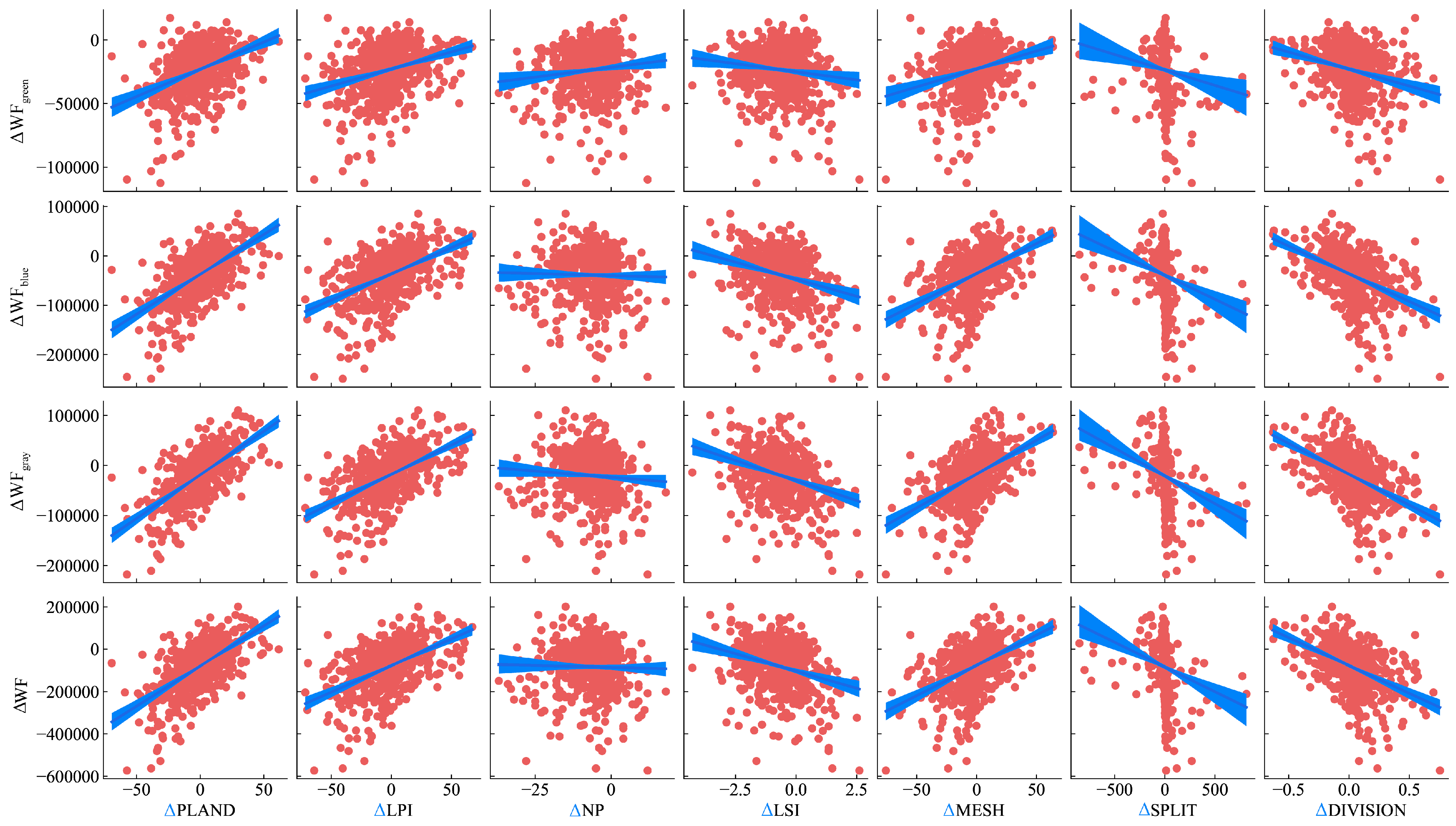
3.3.2. Time-Based Effects of Landscape Metrics on Water Footprint at the Landscape Scale and in WM Patches

At the landscape scale, most of the landscape metrics exhibited a significant influence on the WF (p < 0.001, Figure 4). Regarding the WM patches, ΔPLAND, ΔLPI, ΔLSI, ΔMESH, ΔSPLIT, and ΔDIVISION exhibited significant correlations with ΔWF_blue, ΔWF_green, ΔWF_gray, and ΔWF (p < 0.001, Figure 5).

Within the study area, it was apparent that spatial distribution may exert a more substantial influence, compared to diversification (

Table 1. Time-based effects of landscape metrics on water footprint.

Metrics	Value	Regression Slope/(m3 ha−1 per Unit)				Influence on WF/(m3 ha−1)
		ΔWFgreen	ΔWFblue	ΔWFgray	ΔWF	ΔWFgreen	ΔWFblue	ΔWFgray	ΔWF
At the landscape scale
ΔSHDI	0.07	−172.60 ***	−437.39 ***	−299.87 ***	−909.87 ***	−12.08	−100.62	−90.99	−203.69
ΔED	−3.16	−0.42 ***	−1.18 ***	−0.62 ***	−2.22 ***	1.33	3.73	1.96	7.02
ΔMESH	−5.86	3.10 ***	8.36 ***	7.07 ***	18.54 ***	−18.17	−107.59	−100.03	−225.79
In WM patches
ΔPLAND	−1.14	4.27 ***	16.16 ***	17.40 ***	37.84 ***	−4.87	−18.42	−19.84	−43.13
ΔMESH	−2.32	2.82 ***	12.19 ***	13.51 ***	28.52 ***	−6.54	−28.28	−31.34	−66.16

Notes: *** correlation is significant at p < 0.001.

). At the landscape scale, a variation in SHDI resulted in a reduction in the WF of 203.69 m³ ha⁻¹, while MESH exhibited a larger reduction of 225.79 m³ ha⁻¹. In WM patches, the reduction in PLAND was associated with 23.03 m³ ha⁻¹ less WF, compared to the reduction attributed to MESH.

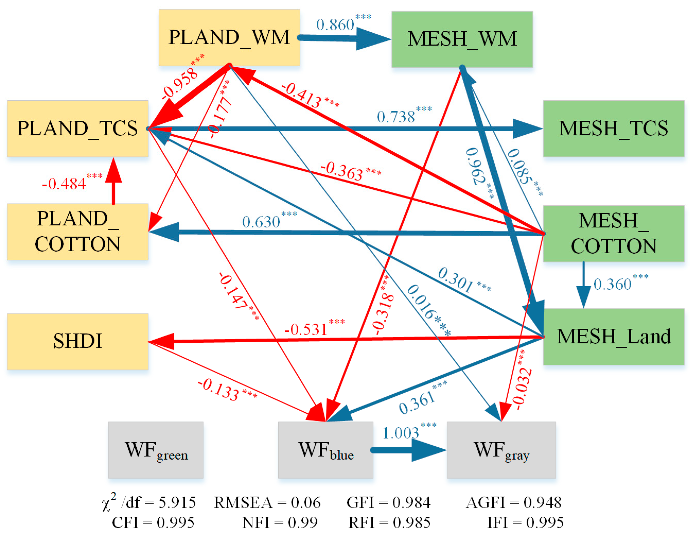
3.3.3. Time-Disregarded Impacts of Landscape Metrics on Water Footprint at the Landscape Scale and in WM Patches

Spatial distribution had a greater influence on WF_blue, compared to diversification (Figure 6). The SEM analysis revealed that diversification had significant negative effects on WF_blue through TCS patches and crop diversity. Conversely, spatial distribution had strong positive effects on WF_blue. Further, spatial distribution of WM patches exerted a strong negative effect on WF_blue.

In addition, the SEM analysis uncovered substantial interactions between different cropping pattern patches and the landscape scale. Specifically, PLAND_WM and PLAND_COTTON exhibited negative effects on PLAND_TCS. MESH_WM and MESH_COTTON demonstrated positive effects on MESH_Land. Moreover, MESH_COTTON exhibited negative effects on PLAND_WM and PLAND_TCS.

4. Discussion

4.1. Diversification and Water Footprint

SHDI and PLAND served as indicators of diversification at the landscape scale and in WM patches, respectively. They exhibited negative effects on water footprint, particularly on WF_blue and WF_gray of the farmland landscape. Notably, the impact of PLAND on WF_blue surpassed that of SHDI. It was similar to previous findings on crop water requirement [15]. This could be attributed to several factors. Firstly, the significant contribution of WM to water footprint, owing to its extensive area, prolonged growth period, and substantial external inputs, implies that reducing the WM planting area while expanding the areas of other cropping patterns, especially those with a lower water footprint, can effectively mitigate the water footprint [42,57,58]. Moreover, the inclusion of supplementary cropping patterns, such as pepper, spring maize, and tree-crop, which exhibit either a small area or low water footprint, enhances crop diversity within subplots and reduces water consumption. Practices like mixed cropping, stripe cropping, rotation, intercropping, and relay cropping are widely acknowledged for improving crop diversification and farmland compositional heterogeneity [59]. These integrated multi-crop arrangements strategically combine crops with varying water requirements in annual or perennial cropping patterns and spatial distributions [58,60]. Lastly, non-crop vegetation exerts minimal water consumption on WF_blue and WF_gray, effectively counterbalancing the negative effects of main cropping patterns at the landscape level. Consequently, the establishment of semi-natural habitats within farmland landscapes emerges as a viable approach for reducing the water footprint.

From a theoretical standpoint, selecting crops/non-crops and cropping patterns characterized by shorter growth periods and reduced external inputs holds the potential to decrease the water footprint in the redesigning of cropping patterns and farmland landscapes. However, the yield of such crops often faces constraints. Therefore, it is crucial to focus on the local objectives of crop production. Pursuing multiple objectives within a single field is unnecessary and can further exacerbate issues related to biodiversity loss and agricultural pollution. A redesign of the farmland landscape becomes imperative. Taking those subplots comprising multiple cropping patterns as examples, WM was chosen to ensure an adequate food supply, and COTTON was selected for fiber production, while TCS and TCD were incorporated to enhance regulation and cultural services. All cropping patterns collectively contribute to achieving a balance between production requirements and environmental sustainability at the landscape scale. Accordingly, determining the appropriate allocation of cropping pattern areas and semi-natural habitats should be based on their favorable characteristics and adverse environmental impacts at the landscape scale. The selection of suitable cropping patterns and semi-natural habitats that strike a balance between production and environmental objectives within the farmland landscape assumes paramount importance in addressing water sustainability in future research endeavors.

4.2. Spatial Distribution and Water Footprint

MESH serves as an indicator of spatial distribution at both the landscape and patch scales, demonstrating a significant negative effect on the water footprint. Field size is a prime influencer of spatial distribution. The positive relationship between field size and MESH suggests that larger field sizes are associated with a higher water footprint in the studied landscapes, which differs from previous research on crop yield and pollination [20,61]. To explain it, the impact of spatial distribution extends beyond agronomic practices to the selection of cropping patterns, thereby influencing the water footprint. Firstly, agronomic management plays a crucial role in reducing water consumption and improving water use efficiency, particularly through optimized irrigation and fertilizer application in fields of varying sizes [62,63]. To balance cost and yield, large-scale field management often entails reducing external inputs per unit area, leading to lower yields. Conversely, smaller field sizes facilitate precision agronomic management with increased inputs to achieve higher yields [64,65,66]. Secondly, larger field sizes result in the reduction and fragmentation of semi-natural habitats, such as flower strips and hedgerows, diminishing their connectivity. This, in turn, hampers pollination, as pollinators need to travel longer distances for foraging and communication, which is different from a water footprint. Lastly, in the context of this intensively managed and biodiversity-limited area, WM emerges as the primary recommended cropping pattern for large-scale production, due to its mechanized cultivation and standardized procedures [66,67,68]. Thus, future research should prioritize the exploration of the interplay among field size, agronomic management, and cropping pattern choice to determine the optimal field size for the redesigning of farmland landscapes.

4.3. Interactive Influences of Landscape Heterogeneity on Water Footprint

MESH exerted greater influences on the water footprint, compared to SHDI, as observed in both the time-based and time-disregarded analyses, highlighting the significant impact of spatial distribution over diversification. This finding aligns with previous studies on biodiversity and pest suppression [69,70,71,72]. They thought that small field size in farmland landscapes could increase the edge density of fields, which could create habitats for animals to survive, such as predators, pollinators, birds, and spiders. However, the underlying reasons differ when considering the water footprint. On the one hand, small field sizes promote the adoption of cropping patterns that are more suitable for less mechanized production, but these patterns are less efficient in terms of water and thermal resource utilization, due to their shorter annual growth period and reduced external inputs, compared to WM. On the other hand, farmers with small fields tend to prioritize high-value cropping patterns over WM to strike a balance between family labor and income. Consequently, landscapes characterized by a higher degree of configurational heterogeneity consist of a larger proportion of cropping patterns with a lower water footprint, leading to an overall reduction in the water footprint at the landscape level. Therefore, further research is warranted to elucidate the mechanisms by which spatial distribution influences crop selection, agronomic management, and ultimately, the water footprint.

It cannot be ignored that mechanization plays a significant role in shaping spatial distribution. On the one hand, the mechanization of all production procedures facilitates the enlargement of field sizes, allowing for a balance among work efficiency, labor costs, and income. On the other hand, unequal development of mechanization across different crops and cropping patterns accentuates variations in field sizes, thereby contributing significantly to farmland landscape heterogeneity. Hence, mechanization directly influences spatial distribution and, in turn, indirectly affects diversification. While this phenomenon is prevalent in many Chinese farmlands, there is an urgent need for further research to quantitatively assess the independent and interdependent influences stemming from landscape heterogeneity.

5. Conclusions

This study provides a novel perspective on enhancing water sustainability through the adjustment of landscape heterogeneity in intensive farming systems. To elucidate the impacts of farmland landscape heterogeneity on the water footprint, spatiotemporal variations in water footprint and landscape pattern metrics were quantitatively analyzed in a representative county. The results revealed that spatial distribution and diversification exerted substantial negative impacts on the water footprint. Notably, spatial distribution, whether operating through direct influence or mediated by diversification, demonstrated a more substantial and comprehensive influence on water footprint. Future research should place an emphasis on investigating the influence of spatial distribution on crop choice and agronomic management to ascertain the optimal cropping patterns and field size that effectively balance crop production and the water footprint. The valuable theoretical guidance and scientific foundation provided by this study offer significant insights for the redesigning of farmland landscapes, with the ultimate goal of enhancing water sustainability in intensive farming systems.

References

1. Tilman, D.; Balzer, C.; Hill, J.; Befort, B.L. Global food demand and the sustainable intensification of agriculture. Proc. Natl. Acad. Sci. USA 2011, 108, 20260–20264. [Google Scholar] [CrossRef] [PubMed]
2. Xiong, L.; Shah, F.; Wu, W. Environmental and socio-economic performance of intensive farming systems with varying agricultural resource for maize production. Sci. Total Environ. 2022, 850, 158030. [Google Scholar] [CrossRef] [PubMed]
3. Hunter, M.C.; Smith, R.G.; Schipanski, M.E.; Atwood, L.W.; Mortensen, D.A. Agriculture in 2050: Recalibrating Targets for Sustainable Intensification. Bioscience 2017, 67, 386–391. [Google Scholar] [CrossRef]
4. Godfray, H.; Beddington, J.R.; Crute, I.R.; Haddad, L.; Lawrence, D.; Muir, J.F.; Pretty, J.; Robinson, S.; Thomas, S.M.; Toulmin, C. Food Security: The Challenge of Feeding 9 Billion People. Science 2010, 327, 812–818. [Google Scholar] [CrossRef] [PubMed]
5. Potts, S.G.; Imperatriz-Fonseca, V.; Ngo, H.T.; Aizen, M.A.; Biesmeijer, J.C.; Breeze, T.D.; Dicks, L.V.; Garibaldi, L.A.; Hill, R.; Settele, J.; et al. Safeguarding pollinators and their values to human well-being. Nature 2016, 540, 220–229. [Google Scholar] [CrossRef]
6. Ju, X.T.; Xing, G.X.; Chen, X.P.; Zhang, S.L.; Zhang, L.J.; Liu, X.J.; Cui, Z.L.; Yin, B.; Christie, P.; Zhu, Z.L.; et al. Reducing environmental risk by improving N management in intensive Chinese agricultural systems. Proc. Natl. Acad. Sci. USA 2009, 106, 3041–3046. [Google Scholar] [CrossRef] [PubMed]
7. Isbell, F.; Adler, P.R.; Eisenhauer, N.; Fornara, D.; Kimmel, K.; Kremen, C.; Letourneau, D.K.; Liebman, M.; Polley, H.W.; Quijas, S.; et al. Benefits of increasing plant diversity in sustainable agroecosystems. J. Ecol. 2017, 105, 871–879. [Google Scholar] [CrossRef]
8. Dainese, M.; Martin, E.A.; Aizen, M.A.; Albrecht, M.; Bartomeus, I.; Bommarco, R.; Carvalheiro, L.G.; Chaplin-Kramer, R.; Gagic, V.; Garibaldi, L.A.; et al. A global synthesis reveals biodiversity-mediated benefits for crop production. Sci. Adv. 2019, 5, eaax0121. [Google Scholar] [CrossRef]
9. Martin, E.A.; Dainese, M.; Clough, Y.; Báldi, A.; Bommarco, R.; Gagic, V.; Garratt, M.P.D.; Holzschuh, A.; Kleijn, D.; Kovács Hostyánszki, A.; et al. The interplay of landscape composition and configuration: New pathways to manage functional biodiversity and agroecosystem services across Europe. Ecol. Lett. 2019, 22, 1083–1094. [Google Scholar] [CrossRef]
10. Tamburini, G.; Bommarco, R.; Wanger, T.C.; Kremen, C.; van der Heijden, M.G.A.; Liebman, M.; Hallin, S. Agricultural diversification promotes multiple ecosystem services without compromising yield. Sci. Adv. 2020, 6, eaba1715. [Google Scholar] [CrossRef]
11. Shi, X.; Xiao, H.; Luo, S.; Hodgson, J.A.; Bianchi, F.J.J.A.; He, H.; van der Werf, W.; Zou, Y. Can landscape level semi-natural habitat compensate for pollinator biodiversity loss due to farmland consolidation? Agric. Ecosyst. Environ. 2021, 319, 107519. [Google Scholar] [CrossRef]
12. Liu, D.; Chen, J.; Ouyang, Z. Responses of landscape structure to the ecological restoration programs in the farming-pastoral ecotone of Northern China. Sci. Total Environ. 2020, 710, 136311. [Google Scholar] [CrossRef] [PubMed]
13. Wang, X.; Wu, Y.; Manevski, K.; Fu, M.; Yin, X.; Chen, F. A Framework for the Heterogeneity and Ecosystem Services of Farmland Landscapes: An Integrative Review. Sustainability 2021, 22, 2463. [Google Scholar] [CrossRef]
14. Fahrig, L.; Baudry, J.; Brotons, L.; Burel, F.G.; Crist, T.O.; Fuller, R.J.; Sirami, C.; Siriwardena, G.M.; Martin, J.L. Functional landscape heterogeneity and animal biodiversity in agricultural landscapes. Ecol. Lett. 2011, 14, 101–112. [Google Scholar] [CrossRef] [PubMed]
15. Han, Y.; Wang, J.; Li, P. Influences of landscape pattern evolution on regional crop water requirements in regions of large-scale agricultural operations. J. Clean. Prod. 2021, 327, 129499. [Google Scholar] [CrossRef]
16. Dadashpoor, H.; Azizi, P.; Moghadasi, M. Land use change, urbanization, and change in landscape pattern in a metropolitan area. Sci. Total Environ. 2019, 655, 707–719. [Google Scholar] [CrossRef] [PubMed]
17. Zang, Z.; Zou, X.Q.; Zuo, P.; Song, Q.C.; Wang, C.L.; Wang, J.J. Impact of landscape patterns on ecological vulnerability and ecosystem service values: An empirical analysis of Yancheng Nature Reserve in China. Ecol. Indic. 2017, 72, 142–152. [Google Scholar] [CrossRef]
18. Liu, Q.F.; Buyantuev, A.; Wu, J.G.; Niu, J.M.; Yu, D.Y.; Zhang, Q. Intensive land-use drives regional-scale homogenization of plant communities. Sci. Total Environ. 2018, 644, 806–814. [Google Scholar] [CrossRef]
19. Beckmann, M.; Gerstner, K.; Akin-Fajiye, M.; Ceausu, S.; Kambach, S.; Kinlock, N.L.; Phillips, H.R.P.; Verhagen, W.; Gurevitch, J.; Klotz, S.; et al. Conventional land-use intensification reduces species richness and increases production: A global meta-analysis. Glob. Chang. Biol. 2019, 25, 1941–1956. [Google Scholar] [CrossRef]
20. Annika, L.; Hass, U.G.K.T. Landscape configurational heterogeneity by small-scale agriculture, not crop diversity, maintains pollinators and plant reproduction in western Europe. Proc. R. Soc. B Biol. Sci. 2018, 285, 20172242. [Google Scholar] [CrossRef]
21. Tilman, D.; Cassman, K.G.; Matson, P.A.; Naylor, R.; Polasky, S. Agricultural sustainability and intensive production practices. Nature 2002, 418, 671–677. [Google Scholar] [CrossRef] [PubMed]
22. Wu, J. Landscape sustainability science (II): Core questions and key approaches. Landsc. Ecol. 2021, 36, 2453–2485. [Google Scholar] [CrossRef]
23. Peng, J.; Liu, Y.; Corstanje, R.; Meersmans, J. Promoting sustainable landscape pattern for landscape sustainability. Landsc. Ecol. 2021, 36, 1839–1844. [Google Scholar] [CrossRef]
24. Kuyah, S.; Sileshi, G.W.; Nkurunziza, L.; Chirinda, N.; Ndayisaba, P.C.; Dimobe, K.; Öborn, I. Innovative agronomic practices for sustainable intensification in sub-Saharan Africa. A Rev. Agron. Sustain. Dev. 2021, 41, 16. [Google Scholar] [CrossRef]
25. Liao, P.; Sun, Y.; Zhu, X.; Wang, H.; Wang, Y.; Chen, J.; Zhang, J.; Zeng, Y.; Zeng, Y.; Huang, S. Identifying agronomic practices with higher yield and lower global warming potential in rice paddies: A global meta-analysis. Agric. Ecosyst. Environ. 2021, 322, 107663. [Google Scholar] [CrossRef]
26. Mekonnen, M.M.; Hoekstra, A.Y. Four billion people facing severe water scarcity. Sci. Adv. 2016, 2, e1500323. [Google Scholar] [CrossRef] [PubMed]
27. Mekonnen, M.M.; Hoekstra, A.Y. The green, blue and grey water footprint of crops and derived crop products. Hydrol. Earth Syst. Sci. 2011, 15, 1577–1600. [Google Scholar] [CrossRef]
28. Hoekstra, A.Y. Virtual water trade. In Proceedings of the International Expert Meeting on Virtual Water Trade, Delft, The Netherlands, 12–13 December 2002. [Google Scholar]
29. Cao, X.; Zeng, W.; Wu, M.; Guo, X.; Wang, W. Hybrid analytical framework for regional agricultural water resource utilization and efficiency evaluation. Agric. Water Manag. 2020, 231, 106027. [Google Scholar] [CrossRef]
30. Hoekstra, A.Y.; Chapagain, A.K.; Aldaya, M.M.; Mekonnen, M.M. Water Footprint Assessment Manual: Setting the Global Standard; Earthscan: London, UK, 2011. [Google Scholar]
31. Novoa, V.; Ahumada-Rudolph, R.; Rojas, O.; Saez, K.; de la Barrera, F.; Luis Arumi, J. Understanding agricultural water footprint variability to improve water management in Chile. Sci. Total Environ. 2019, 670, 188–199. [Google Scholar] [CrossRef] [PubMed]
32. Xu, Z.; Chen, X.; Wu, S.R.; Gong, M.; Du, Y.; Wang, J.; Li, Y.; Liu, J. Spatial-temporal assessment of water footprint, water scarcity and crop water productivity in a major crop production region. J. Clean. Prod. 2019, 224, 375–383. [Google Scholar] [CrossRef]
33. Zhao, Y.; Ding, D.; Si, B.; Zhang, Z.; Hu, W.; Schoenau, J. Temporal variability of water footprint for cereal production and its controls in Saskatchewan, Canada. Sci. Total Environ. 2019, 660, 1306–1316. [Google Scholar] [CrossRef] [PubMed]
34. Wang, X.; Jia, R.; Zhao, J.; Yang, Y.; Zang, H.; Zeng, Z.; Olesen, J.E. Quantifying water footprint of winter wheat–summer maize cropping system under manure application and limited irrigation: An integrated approach. Resour. Conserv. Recycl. 2022, 183, 106375. [Google Scholar] [CrossRef]
35. Wang, J.; Qin, L.; Li, B.; Dang, Y. Assessing the hotspots of crop water footprint in Jilin Province of China. Env. Sci. Pollut. Res. Int. 2022, 29, 50010–50024. [Google Scholar] [CrossRef] [PubMed]
36. Kashyap, D.; Agarwal, T. Carbon footprint and water footprint of rice and wheat production in Punjab, India. Agric. Syst. 2021, 186, 102959. [Google Scholar] [CrossRef]
37. Chouchane, H.; Krol, M.S.; Hoekstra, A.Y. Changing global cropping patterns to minimize national blue water scarcity. Hydrol. Earth Syst. Sci. 2020, 24, 3015–3031. [Google Scholar] [CrossRef]
38. Li, H.; Wang, Y.; Qin, L.; He, H.; Zhang, T.; Wang, J.; Zheng, X. Effects of different slopes and fertilizer types on the grey water footprint of maize production in the black soil region of China. J. Clean. Prod. 2020, 246, 119077. [Google Scholar] [CrossRef]
39. Dong, H.; Zhang, L.; Geng, Y.; Li, P.; Yu, C. New insights from grey water footprint assessment: An industrial park level. J. Clean. Prod. 2021, 285, 124915. [Google Scholar] [CrossRef]
40. Fu, T.; Xu, C.; Yang, L.; Hou, S.; Xia, Q. Measurement and driving factors of grey water footprint efficiency in Yangtze River Basin. Sci. Total Environ. 2022, 802, 149587. [Google Scholar] [CrossRef] [PubMed]
41. Zhang, S.; Liu, Y.; Zhang, K.; Jiang, Y. Study on Quality Evaluation of County Cultivated Land Based on Information Technology. J. Anhui Agric. Sci. 2008, 36, 8202–8204. [Google Scholar] [CrossRef]
42. Chen, X.; Wang, P.; Muhammad, T.; Xu, Z.; Li, Y. Subsystem-level groundwater footprint assessment in North China Plain–The world’s largest groundwater depression cone. Ecol. Indic. 2020, 117, 106662. [Google Scholar] [CrossRef]
43. Zhang, E.; Yin, X.; Yang, Z. Contributions of climate change and human activities to changes in the virtual water content of major crops: An assessment for the Shijiazhuang Plain, northern China. Resour. Conserv. Recycl. 2021, 169, 105498. [Google Scholar] [CrossRef]
44. Feng, W.; Shum, C.; Zhong, M.; Pan, Y. Groundwater Storage Changes in China from Satellite Gravity: An Overview. Remote Sens. 2018, 10, 674. [Google Scholar] [CrossRef]
45. DWRHP (Department of Water Resources of Hebei Province). Heibei Water Resources Bulletin. 2020. Available online: http://slt.hebei.gov.cn/a/2021/08/04/F3A8F2A53BD44494B6F0A253372F4530.html (accessed on 10 January 2022).
46. BSW (Bureau of Statistics in Wuqiao). Yearbook of Wuqiao; Bureau of Statistics in Wuqiao: Shijiazhuang, China, 2019.
47. Wang, X.; Jiang, Y.; Fu, M.; Yin, X.; Chen, F. Cropping patterns and farmland landscape at the county level using remote sensing in Haihe Lowland Plain. Trans. CSAE. 2022, 38, 297–304. Available online: http://www.tcsae.org/article/doi/10.11975/j.issn.1002-6819.2022.01.033 (accessed on 8 July 2024).
48. Duflot, R.; Ernoult, A.; Aviron, S.; Fahrig, L.; Burel, F. Relative effects of landscape composition and configuration on multi-habitat gamma diversity in agricultural landscapes. Agric. Ecosyst. Environ. 2017, 241, 62–69. [Google Scholar] [CrossRef]
49. Meier, E.S.; Luescher, G.; Knop, E. Disentangling direct and indirect drivers of farmland biodiversity a landscape scale. Ecol. Lett. 2022, 25, 2422–2434. [Google Scholar] [CrossRef] [PubMed]
50. Allen, R.G.; Pereira, L.S.; Raes, D.; Smith, M. Crop Evapotranspiration: Guidelines for Computing Crop Water Requirement; Food and Agriculture Organization of the United Nations: Rome, Italy, 1998. [Google Scholar]
51. Ren, T.; Liu, H.; Fan, X.; Zou, G.; Liu, S. Handbook on Emission Factors of Agricultural Non-Point Source Pollution in China; China Agriculture Press: Beijing, China, 2015. [Google Scholar]
52. Farina, A. Principles and Methods in Landscape Ecology: Towards a Science of the Landscape; Springer Science & Business Media: Berlin/Heidelberg, Germany, 2008. [Google Scholar]
53. Syrbe, R.; Walz, U. Spatial indicators for the assessment of ecosystem services: Providing, benefiting and connecting areas and landscape metrics. Ecol. Indic. 2012, 21, 80–88. [Google Scholar] [CrossRef]
54. Sklenicka, P.; Janovska, V.; Salek, M.; Vlasak, J.; Molnarova, K. The Farmland Rental Paradox: Extreme land ownership fragmentation as a new form of land degradation. Land. Use Policy 2014, 38, 587–593. [Google Scholar] [CrossRef]
55. Wei, L.; Luo, Y.; Wang, M.; Su, S.; Pi, J.; Li, G. Essential fragmentation metrics for agricultural policies: Linking landscape pattern, ecosystem service and land use management in urbanizing China. Agric. Syst. 2020, 182, 102833. [Google Scholar] [CrossRef]
56. Šímová, P.; Gdulová, K. Landscape indices behavior: A review of scale effects. Appl. Geogr. 2012, 34, 385–394. [Google Scholar] [CrossRef]
57. Chu, Y.; Shen, Y.; Yuan, Z. Water footprint of crop production for different crop structures in the Hebei southern plain, North China. Hydrol. Earth Syst. Sci. 2017, 21, 3061–3069. [Google Scholar] [CrossRef]
58. Chen, Y.; Zhou, Y.; Fang, S.; Li, M.; Wang, Y.; Cao, K. Crop pattern optimization for the coordination between economy and environment considering hydrological uncertainty. Sci. Total Environ. 2022, 809, 151152. [Google Scholar] [CrossRef]
59. Weltin, M.; Zasada, I.; Piorr, A.; Debolini, M.; Geniaux, G.; Perez, O.M.; Scherer, L.; Marco, L.T.; Schulp, C. Conceptualising fields of action for sustainable intensification-A systematic literature review and application to regional case studies. Agric. Ecosyst. Environ. 2018, 257, 68–80. [Google Scholar] [CrossRef]
60. Cao, X.; Zeng, W.; Wu, M.; Li, T.; Chen, S.; Wang, W. Water resources efficiency assessment in crop production from the perspective of water footprint. J. Clean. Prod. 2021, 309, 127371. [Google Scholar] [CrossRef]
61. Magrach, A.; Giménez García, A.; Allen Perkins, A.; Garibaldi, L.A.; Bartomeus, I. Increasing crop richness and reducing field sizes provide higher yields to pollinator-dependent crops. J. Appl. Ecol. 2023, 60, 77–90. [Google Scholar] [CrossRef]
62. Benedetti, I.; Branca, G.; Zucaro, R. Evaluating input use efficiency in agriculture through a stochastic frontier production: An application on a case study in Apulia (Italy). J. Clean. Prod. 2019, 236, 117609. [Google Scholar] [CrossRef]
63. Medrano, H.; Tomas, M.; Martorell, S.; Escalona, J.; Pou, A.; Fuentes, S.; Flexas, J.; Bota, J. Improving water use efficiency of vineyards in semi-arid regions. A Rev. Agron. Sustain. Dev. 2015, 35, 499–517. [Google Scholar] [CrossRef]
64. Ricciardi, V.; Mehrabi, Z.; Wittman, H.; James, D.; Ramankutty, N. Higher yields and more biodiversity on smaller farms. Nat. Sustain. 2021, 4, 651–657. [Google Scholar] [CrossRef]
65. Liebert, J.; Benner, R.; Kerr, R.B.; Bjorkman, T.; De Master, K.T.; Gennet, S.; Gomez, M.I.; Hart, A.K.; Kremen, C.; Power, A.G.; et al. Farm size affects the use of agroecological practices on organic farms in the United States. Nat. Plants. 2022, 8, 897–905. [Google Scholar] [CrossRef]
66. Wang, C.; Duan, J.; Ren, C.; Liu, H.; Reis, S.; Xu, J.; Gu, B. Ammonia Emissions from Croplands Decrease with Farm Size in China. Environ. Sci. Technol. 2022, 56, 9915–9923. [Google Scholar] [CrossRef]
67. Skalos, J.; Molnarova, K.; Kottova, P. Land reforms reflected in the farming landscape in East Bohemia and in Southern Sweden-Two faces of modernisation. Appl. Geogr. 2012, 35, 114–123. [Google Scholar] [CrossRef]
68. Ren, C.; Jin, S.; Wu, Y.; Zhang, B.; Kanter, D.; Wu, B.; Xi, X.; Zhang, X.; Chen, D.; Xu, J.; et al. Fertilizer overuse in Chinese smallholders due to lack of fixed inputs. J. Environ. Manag. 2021, 293, 112913. [Google Scholar] [CrossRef]
69. Fahrig, L.; Girard, J.; Duro, D.; Pasher, J.; Smith, A.; Javorek, S.; King, D.; Lindsay, K.F.; Mitchell, S.; Tischendorf, L. Farmlands with smaller crop fields have higher within-field biodiversity. Agric. Ecosyst. Environ. 2015, 200, 219–234. [Google Scholar] [CrossRef]
70. Martin, E.A.; Seo, B.; Park, C.R.; Reineking, B.; Steffan-Dewenter, I. Scale-dependent effects of landscape composition and configuration on natural enemy diversity, crop herbivory, and yields. Ecol. Appl. 2016, 26, 448–462. [Google Scholar] [CrossRef] [PubMed]
71. Zhang, Y.; Haan, N.L.; Landis, D.A. Landscape composition and configuration have scale-dependent effects on agricultural pest suppression. Agric. Ecosyst. Environ. 2020, 302, 107085. [Google Scholar] [CrossRef]
72. Thomine, E.; Rusch, A.; Desneux, N. Predators do not benefit from crop diversity but respond to configurational heterogeneity in wheat and cotton fields. Landsc. Ecol. 2023, 38, 439–447. [Google Scholar] [CrossRef]
Figure 1. Water footprints of crops (a) and cropping patterns (b). Notes: WFgreen: green water footprint; WFblue: blue water footprint; WFgray: gray water footprint; WM: winter wheat–summer maize double cropping pattern; COTTON: cotton single cropping pattern; PEPPER: pepper single cropping pattern; MAIZE: spring maize single cropping pattern; PEANUT: peanut single cropping pattern; TCS: tree crop single cropping; TCD: tree crop double cropping.
Land 13 01042 g001
Figure 2. Variations in water footprints and landscape pattern metrics of 616 subplots. SHDI, PLAND, and LPI demonstrated diversification. ED, NP, and LSI demonstrated fragmentation. MESH, SPLIT, and DIVISION demonstrated spatial distribution. Notes: WFgreen: green water footprint; WFgray: gray water footprint; WFblue: blue water footprint; WF: crop water footprint; SHDI: Shannon’s diversity index; PLAND: percentage of landscape of the WM patches; LPI: largest patch index; ED: edge density; NP: number of patches; LSI: landscape shape index; MESH: effective mesh size; SPLIT: splitting index; DIVISION: landscape division index.
Land 13 01042 g002
Figure 3. Correlations among landscape pattern metrics and water footprints. (a,b) shows correlations among landscape pattern metrics and water footprints at the landscape scale. (c,d) shows the correlations of the winter wheat–summer maize double cropping pattern. Notes: SHDI: Shannon’s diversity index; PLAND: percentage of landscape of the WM patches; LPI: largest patch index; ED: edge density; NP: number of patches; LSI: landscape shape index; MESH: effective mesh size; SPLIT: splitting index; DIVISION: landscape division index; WFblue: blue water footprint; WFgreen: green water footprint; WFgray: gray water footprint; WF: crop water footprint; The colors of the blocks represent the value of the correlation coefficient; * correlation is significant at p < 0.05; ** correlation is significant at p < 0.01; *** correlation is significant at p < 0.001.
Land 13 01042 g003
Figure 4. Linear regression analysis of landscape pattern metrics and the water footprint at the landscape scale during the years 2013–2019. Red points are differences of the landscape pattern metrics or water footprint between the two years. Each point is a subplot. The blue line and interval show the linear regression of pattern metrics and water footprint. Notes: SHDI: Shannon’s diversity index; LPI: largest patch index; ED: edge density; LSI: landscape shape index; MESH: effective mesh size; SPLIT: splitting index; DIVISION: landscape division index; WFblue: blue water footprint; WFgreen: green water footprint; WFgray: gray water footprint; WF: crop water footprint.
Land 13 01042 g004
Figure 5. Linear regression analysis of landscape pattern metrics and water footprint in WM patches during the years 2013–2019. Red points are differences of the landscape pattern metrics or water footprint between the two years. Each point is a subplot. The blue line and interval show the linear regression of pattern metrics and water footprint. Notes: PLAND: percentage of landscape; LPI: largest patch index; NP: number of patches; LSI: landscape shape index; MESH: effective mesh size; SPLIT: splitting index; DIVISION: landscape division index; WFblue: blue water footprint; WFgreen: green water footprint; WFgray: gray water footprint; WF: crop water footprint.
Land 13 01042 g005
Figure 6. Time-disregarded impacts of landscape metrics on water footprint through SEM analysis. Notes: Yellow, green, and gray boxes contain diversification, spatial distribution, and water footprint indicators, respectively. Red and blue solid arrows reflect negative and positive correlations, respectively. Standardized path coefficients are presented adjacent to the arrows. PLAND_WM: percentage of landscape of WM patches; PLAND_TCS: percentage of landscape of TCS patches; PLAND_COTTON: percentage of landscape of COTTON patches; SHDI: Shannon’s diversity index; MESH_WM: effective mesh size of WM patches; MESH_TCS: effective mesh size of TCS patches; MESH_COTTON: effective mesh size of COTTON patches; MESH_Land: effective mesh size of an entire subplot. WFgreen: green water footprint; WFblue: blue water footprint; WFgray: gray water footprint. *** correlation is significant at p < 0.001.
Land 13 01042 g006