Spatial and Temporal Dynamics and Multi-Scenario Forecasting of Habitat Quality in Gansu–Qinghai Contiguous Region of the Upper Yellow River

Abstract

Human activities exert a profound influence on land use and land cover, and these changes directly influence habitat quality and ecosystem functioning. In the Gansu–Qinghai contiguous region of the upper Yellow River, habitat quality has undergone substantial transformations in recent years due to the synergistic impacts of natural processes and human intervention. Therefore, evaluating the effects of land use changes on habitat quality is crucial for advancing regional sustainable development and improving the worth of ecosystem services. In response to these challenges, we devised a two-pronged approach: a land use simulation (FLUS) model and an integrated valuation of ecosystem services and trade-offs (InVEST) model, leveraging remote sensing data. This integrated methodology establishes a research framework for the evaluation and simulation of spatial and temporal variations in habitat quality. The results of the study show that, firstly, from 1980 to 2020, the habitat quality index in the Gansu–Qinghai contiguous region of the upper Yellow River decreased from 0.8528 to 0.8434. Secondly, our predictions anticipate a decrease in habitat quality, although the decline is not pronounced across all scenarios. The highest habitat quality values were projected under the EP (Ecology Priority) scenario, followed by the CLP (Cultivated Land Priority) scenario, while the BAU (Business as Usual) scenario consistently yielded the lowest values in all three scenarios. Finally, the ecological land, including forest land and grassland, consistently occupied areas characterized by high habitat quality. In contrast, Construction land consistently appeared in regions associated with low habitat quality. The implementation of conservation measures emerges as a crucial strategy, effectively limiting the expansion of construction land and promoting the augmentation of forest land and grassland cover. This approach serves to enhance overall habitat quality. These outcomes furnish a scientific foundation for the judicious formulation of future land-use policies and ecological protection measures.

1. Introduction

The expansion of urban areas and heightened human activity have led to a significant decline in biodiversity, habitat fragmentation, and the deterioration of ecosystems [1]. Presently, urban areas across the globe are expanding at an average rate twice as fast as their populations [2,3]. Changes in land cover could result in the loss of up to 40% of species in some of the most biologically diverse regions worldwide, and by 2000, 88% of the primary vegetation land cover in biodiversity hotspots had been destroyed [4]. Habitat quality serves as a reliable metric for assessing biodiversity, providing insights into the overall health of ecosystems [5,6]. In light of the ongoing trend of ecological degradation, it becomes imperative to anticipate and model habitat quality under prospective ecological conservation scenarios [7,8].

Researchers both domestically and internationally have utilized various models to simulate future land-use scenarios and changes in habitat quality, enabling the visualization of projections from different perspectives and at different scales, which also involve the intricate relationship between land use and habitat quality. At the watershed scale, Wei et al. [9] analyzed spatial and temporal changes in habitat quality by integrating fine-scale processes, such as land use, into a large-scale ecosystem framework. They concluded that irrational development activities can lead to the deterioration of habitat quality and the loss of biodiversity, especially in arid inland areas with fragile ecosystems. Yang et al. [10] highlighted the challenges faced by habitats, emphasizing that the quality and degradation of habitats hinge on the location and intensity of anthropogenic effects, displaying sensitivity to varying levels of protection. In their analysis of the connection between land use and habitat, Tang et al. [11] took a new perspective, and explored the spatial and temporal differentiation characteristics of habitat quality within the context of ecological civilization and the construction of ecologically livable cities. While existing research has made great strides in the content, methods, and ideas related to habitat quality, certain deficiencies persist. Firstly, there is a limitation in research time, as the temporal spans in existing studies are not sufficiently broad to comprehensively capture the space–time evolution of habitat. Secondly, from a research perspective, there is a notable scarcity in studies that integrate land use prediction models with habitat quality models, hindering a comprehensive understanding of the coupling dynamics between these two crucial elements [12,13].

The assessment of future land’s current habitat conditions is facilitated by the FLUS-InVEST model, offering a valuable tool for land use planners. The most widely used land use simulation models include the Markov Model, Cellular Automata (CA) model, Multi-Agent-System (MAS) model, effects of changing land use model (CLUE-S: Conversion of Land Use and its Effects at Small Region Extent), the system simulation (System Dynamics, SD) model, the Artificial Neural Network (ANN) model, and the FLUS model [14], which have applications in land use change and its environmental effects, as well as land use policy research. However, many of these models have certain limitations. For instance, the Cellular Automata (CA) model makes insufficient consideration of the impacts of various macro factors on simulation results [15], the Multi-Agent-System (MAS) model overly emphasizes the influence of human activities on simulation results, the CLUE-S model is particularly sensitive to iterative variables and land use conversion elastic coefficients, and the Artificial Neural Network (ANN) emphasizes economic benefits and its selection of network structure differs [16]. In contrast, the FLUS model combines top-down macro-prediction and bottom-up micro-simulation, and is able to simulate land use changes under the influence of natural and human activities very well [17]. The FLUS model combines an artificial neural network algorithm and an adaptive inertia wheel mechanism; the former effectively solves the nonlinear relationship between drivers with high accuracy (http://www.geosimulation.cn/FLUS.html, accessed on 13 February 2024), and the latter employs a wheel selection mechanism with stochastic characteristics, which is able to effectively reflect the switching time within the prefecture-level cities’ competitive relationship [18]. The prevailing trend in ecological assessment leans towards quantitative and refined methodologies, with notable models such as the InVSET model, HSI model, and MAXENT model [19,20]. The InVSET model, in particular, overcomes non-spatial valuation limitations, analyzing the impacts of diverse threat factors and land use changes on local biodiversity at multiple scales. Furthermore, it presents assessment results in an intuitive manner [21,22]. The InVSET model’s strength lies in its ability to integrate ecosystem services, such as hydrological services and climate regulation, with land use changes [23]. This integration equips policymakers with information on the potential ecological benefits and environmental impacts associated with different programs.

The quantification of the impact of land use on habitat quality in the Gansu–Qinghai contiguous region of the upper Yellow River is pivotal for comprehending how shifts in habitat quality, projected under future change scenarios, will influence this critical region [24,25]. Specifically, the Gansu–Qinghai contiguous region of the upper Yellow River, situated in the Qinghai–Tibet Plateau and the Loess Plateau regions, exhibits diverse climate conditions [26]. This area holds strategic significance for ecological preservation and plays a crucial role in the broader biodiversity conservation strategy [27,28]. While acknowledging the evolution of the Yellow River’s habitat quality pattern and forecasting its future trajectory, our study seeks to address the following key objectives: (1) To analyze the evolutionary processes and patterns of habitat quality in the region spanning from 1980 to 2020. (2) To simulate the temporal changes in habitat quality for the future period. This endeavor aims to furnish a reliable scientific foundation for shaping future land use policies and ecological protection measures. Moreover, the insights gained from this study aspire to offer valuable experiences and references for promoting sustainable development and ecological restoration in other ecologically fragile areas.

2. Materials and Methods

2.1. Study Area

The Gansu–Qinghai contiguous region of the upper Yellow River is located in the Qinghai–Tibet Plateau and the Loess Plateau, with an average altitude between 1300 m and 6180 m (Figure 1). This region’s landform is mainly grassland, covering a total area of 234,100 km², accounting for about 2.4% of the land area. It encompasses 68 districts and counties, including those in Lanzhou, Baiyin, Linxia, Gannan, Wuwei’s Tianzhu County, Dingxi’sAnding District, Longxi County, Weiyuan County, Lintao, Zhang and Min, Xining, Haidong and Haibei in Qinghai Province, as well as those in Hainan, Huangnan, Guoluo, Yushu’s duo County and Qumalai County. The geographical environment and climate conditions are relatively complex; it is located in the transitional area between the high-altitude plateau and temperate continental climates. There is considerable spatial variability in the distribution of average annual precipitation. Grasslands are the dominant vegetation type, but the region’s diverse climate, deep steep valleys and fragile ecosystems make it a critical and challenging area for ecological conservation.

2.2. Data Source and Processing

The necessary data for this study are detailed in

Table 1. Data source and relative data descriptions.

Categories	Data Name	Data Type	Data Source
Land Use Data	Land Use/Land Cover	Grid	Resource and Environmental Data Sharing Center of Chinese Academy of Sciences (http://www.resdc.cn/, accessed on 13 March 2024)
Natural Environment Data	Dem	Grid	Resource and Environmental Data Sharing Center of Chinese Academy of Sciences (http://www.resdc.cn/, accessed on 13 March 2024)
	Slope	Grid	Elevation data was obtained after slope processing in GIS
	Aspect
	Precipitation, Evaporation	Grid	NASA Dataset (https://data.tpdc.ac.cn, accessed on 14 March 2024)
Socio-economic Data	Distance from town center, city center	Shapefile	Openstreetmap dataset (https://www.openstreetmap.org, accessed on 15 March 2024)
	Distance from main road, railroad, highway	Shapefile	Openstreetmap dataset (https://www.openstreetmap.org, accessed on 15 March 2024)

. The processing, spatial and statistical analyses of the data set were conducted using ArcGIS10.8 and its associated tools.

The different indicators selected for normalization were: elevation, slope, aspect, precipitation, evaporation, distance from main road, railroad and highway, and distance from city center and town center. Five natural and five socio-economic factors were included as drivers of habitat quality and factor data for model simulations. Data sources for specific factors are shown in Table 1. Land use data (derived from the multi-period remote sensing land use monitoring data set), DEM data, and vector data such as administrative area boundaries were obtained from the Chinese Academy of Sciences and the China Resource and Environmental Science Data Center (http://www.resdc.cn, accessed on 13 March 2024). In line with China’s current land resource classification system and the aims of this study, land use categories are delineated as: cultivated land, forest land, grassland, water, construction land and unused land. Precipitation and evapotranspiration data were downloaded from the Tibetan Plateau Data Center (https://data.tpdc.ac.cn, accessed on 14 March 2024). Five socio-economic factors were obtained from the Openstreetmap dataset (https://www.openstreetmap.org, accessed on 15 March 2024). Euclidean distance operations were performed to set the buffer for distance-making. A sequence of procedures was executed to procure the fundamental spatial data, including Euclidean distance calculation, image cropping, masking, and reclassification. Furthermore, the spatial data set was aligned to the Krasovosky_1940_Albers coordinate framework using a projection tool, ensuring uniformity in the number of spatial raster columns and rows across all grid data. To preserve data uniformity, the spatial resolution was resampled to a 30 m grid size (Table 1).

2.3. Research Method

2.3.1. The Research Framework

Based on land use data, we obtained the quantity of land use types under different scenarios in 2030 and 2040 using the Markov model. With all the data prepared, we simulated land use patterns in 2030 and 2040 under three scenarios using the FLUS model. Then, we estimated the habitat quality of the Gansu–Qinghai contiguous region of the upper Yellow River during 1980–2040 based on the InVEST model. The research framework is shown in Figure 2.

The importance of integrating the FLUS model with the InVEST model lies in their ability to provide complementary information for a more comprehensive understanding of the effects of land use change on ecosystems and their habitat quality. Via this research process, the integration of the FLUS-InVEST model is reflected in the following aspects: First, model construction and calibration. The FLUS model was selected as the land use prediction model and the InVEST model was used to assess habitat quality, and the two models were calibrated and validated using historical data to ensure the accuracy and reliability of the models, which were validated in this study by comparing actual and simulated land use in 2020. Second, the model interface. The outputs of the land use projection model were used as inputs to the habitat quality model, and the projected 2030 and 2040 land use data were used as input data for habitat quality in this study. Third, scenario analysis. Different land use change scenarios were generated using the land use prediction model, and these scenarios were used as inputs to assess the changes in habitat quality under different scenarios through the InVEST model, and the changes in habitat quality under three scenarios were assessed in this study. The effects of different scenarios on habitat quality were analyzed and critical areas were identified.

2.3.2. Scenario Setting

The Gansu–Qinghai contiguous region of the upper Yellow River has diverse climates, different social conditions, and diverse land use patterns. Here is a structured summary of the three scenarios used in the study to predict land use demand and spatial layout in 2040, taking into account different development goals, potential disturbances and policy drivers:

(1) Business as Usual (BAU) Scenario. This scenario assumes the continuation of historical trends in urban expansion without considering national land use planning constraints and policy influences. It is independent of the rate of socio-economic development. It projects that the land use trends from 2020 to 2040 will follow the same patterns observed from 2010 to 2020;

(2) Cultivated Land Priority (CLP) Scenario. The CLP scenario focuses on the protection of basic farmland, imposes strict limitations on the conversion of cultivated land to other land types, and aims to protect cultivated land from being overtaken by urban expansion during economic development. It specifically curtails the transformation of cultivated land to other classes, and sets restrictions on conversions such as forest land to water, grassland to cultivated land, and water to forest land and construction land;

(3) Ecological Priority (EP) Scenario. Under the EP scenario, ecological benefits are prioritized to enhance ecosystem protection and restoration efforts, thereby minimizing the encroachment on ecological lands. With the goal of “restoring important ecosystems and strengthening water conservation functions”, the ecological redline areas are designated as areas where land conversion is prohibited. However, outside the ecological redline areas, the probability of converting arable land, grassland, forest land, and water to construction land is reduced by 35%, 50%, 50%, and 10%, respectively. Ecological land such as forest land, grassland, and water are prohibited from being converted to unused land. At the same time, forest land and water are no longer allowed to be converted to other land use types, while grassland can be converted to forest land and water, but not to other land use types.

2.3.3. FLUS Model

The FLUS model (GeoSOS-FLUS V2.4) is an integrative tool that assimilates both human and natural factors to simulate different land use scenarios [28,29]. Initially, the model employs an artificial neural network algorithm to process the baseline period’s land use data and array of driving factors, thereby calculating the suitability probability for each land type. Subsequently, this suitability probability is combined with the neighborhood factor, an adaptive inertia coefficient, and a cost matrix to refine the model’s parameters. Finally, by examining the intricate dynamics of land use alterations under the influence of various driving factors, we can extract simulated outcomes of land use changes [30].

(1) Estimation of the suitability probability using artificial neural networks

An artificial neural network (ANN) is a machine learning model inspired by biological neural networks [31]. It has been widely applied in the analysis and simulation of complex, nonlinear problems in geography. An ANN typically involves two key phases: training and prediction. During the training phase, the goal is to determine the appropriate weights for different land use types. In the prediction phase, the objective is to estimate the probability distribution of the spatial arrangement of various land types. The specific formula of an artificial neural network (ANN) is as follows:

$$\mathrm{p}\left(\mathrm{p},\mathrm{k},\mathrm{t}\right)={\displaystyle {\sum }_{\mathrm{j}}{\mathrm{w}}_{\mathrm{j},\mathrm{k}}}\times \frac{1}{1+{\mathrm{e}}^{-{\mathrm{net}}_{\mathrm{j}\left(\mathrm{p},\mathrm{t}\right)}}}$$

where ${\mathrm{net}}_{\mathrm{j}\left(\mathrm{k},\mathrm{t}\right)}$ represents the suitability probability of land use type $\mathrm{k}$ on grid $\mathrm{p}$ at time $\mathrm{t}$, and ${\mathrm{w}}_{\mathrm{j},\mathrm{k}}$ are the adaptive weights between the hidden layer and the output layer, which are fine-tuned during the training process. The term ${\mathrm{net}}_{\mathrm{j}\left(\mathrm{k},\mathrm{t}\right)}$ denotes that neuron $\mathrm{j}$ receives signals from all of the input neurons on grid $\mathrm{p}$ at time $\mathrm{t}$ in the hidden layer. In the output of the neural network, the sum of the suitability probability for all land use types equals 1 for each grid $\mathrm{p}$ at each iteration time $\mathrm{t}$.

(2) Cellular automata with an adaptive inertial mechanism

The transition of a land grid to a specific land use type is influenced not only by the occurrence probability but also by various other factors that represent different development states during the forecast period [32]. The essence of the adaptive inertial competition mechanism lies in the adaptive coefficient. This coefficient modulates the transition probabilities of the current land type in the subsequent iteration to achieve the anticipated developmental objectives.

$${\mathrm{Interia}}_{\mathrm{k}}^{\mathrm{t}}\left\{\begin{array}{l}{\mathrm{Interia}}_{\mathrm{k}}^{\mathrm{t}-1} \mathrm{if} \left|{\mathrm{D}}_k^{\mathrm{t}-2}\right|\le \left|{\mathrm{D}}_k^{\mathrm{t}-1}\right|\\ {\mathrm{Interia}}_{\mathrm{k}}^{\mathrm{t}-1}\times \frac{{\mathrm{D}}_k^{\mathrm{t}-2}}{{\mathrm{D}}_k^{\mathrm{t}-1}} \mathrm{if} 0>\left|{\mathrm{D}}_k^{\mathrm{t}-2}\right|>\left|{\mathrm{D}}_k^{\mathrm{t}-1}\right|\\ {\mathrm{Interia}}_k^{\mathrm{t}-1}\times \frac{{\mathrm{D}}_k^{\mathrm{t}-2}}{{\mathrm{D}}_k^{\mathrm{t}-1}} \mathrm{if} \left|{\mathrm{D}}_k^{\mathrm{t}-1}\right|>\left|{\mathrm{D}}_k^{\mathrm{t}-2}\right|>0\end{array}\right.\mathrm{k}$$

where ${\mathrm{Interia}}_{\mathrm{k}}^{\mathrm{t}}$ is the coefficient of inertia of land type $\mathrm{k}$. At iteration $\mathrm{t}-1$ and $\mathrm{t}-2$, ${\mathrm{D}}_k^{\mathrm{t}-1}$ and ${\mathrm{D}}_k^{\mathrm{t}-2}$ are the differences between the requested land quantity for a specific type of land ($\mathrm{k}$) and the actual amount of that land available.

(3) Neighbor factor

The establishment and protection of nature reserves restrict the expansion potential of construction land while bolstering the expansion capabilities of woodlands and grasslands [33]. To determine the parameters, a comparative analysis of neighborhood factor parameters is conducted before and after the implementation of the current scheme. These neighborhood coefficients quantify the interactions among various land use types. The values of proximity parameter coefficients, which range from 0 to 1, indicate the expansion propensity of land types under the influence of different factors [34]. A value closer to 1 suggests a stronger ability of a land type to expand. Informed by prior research and the regulatory framework provided by regulations of the People’s Republic of China on Nature Reserves, the Protection Plan of National Key Ecological Function areas and the Land Administration Law of the People’s Republic of China, the neighborhood factor parameters of land use types are set (

Table 2. Neighborhood factor parameters for different scenarios.

Land Use Type *		1	2	3	4	5	6
BAU		0.5	0.7	0.3	0.4	0.9	0.1
CLP		0.8	0.6	0.3	0.4	0.7	0.1
EP		0.3	1	0.7	0.5	0.7	0.1

* 1 cultivated land, 2 forest land, 3 grassland, 4 water, 5 construction land, 6 unused land.

).

(4) Cost transfer matrix for different scenario

The conversion cost matrix quantifies the difficulty associated with the transformation between different land use types [35]. A value 0 indicates no conversion resistance, and 1 signifies complete convertibility [36]. Reflecting the dynamics of actual land use changes, the construction cost matrix for construction land is set to 0. This is because, during economic development, other land types are frequently converted into construction land. The cost matrix of other land types is determined based on the conversion constraints that exist among different land types under various scenarios (

Table 3. Conversion cost matrix under three scenarios.

Land Use Type *	Scenario1 (BAU)						Scenario2 (CLP)						Scenario3 (EP)
	1	2	3	4	5	6	1	2	3	4	5	6	1	2	3	4	5	6
Cultivated Land	1	1	1	1	1	1	1	0	0	0	0	0	1	1	1	1	1	1
Forest Land	1	1	1	1	1	1	1	1	1	0	1	1	0	1	0	0	0	0
Grassland	1	1	1	1	1	1	0	1	1	1	1	1	0	1	1	1	0	0
Water	1	1	1	1	1	1	1	0	1	1	0	1	0	0	0	1	0	0
Construction Land	0	0	0	0	1	0	0	0	0	0	1	0	0	0	0	0	1	0
Unused Land	1	1	1	1	1	1	1	1	1	1	1	1	1	1	1	1	1	1

* 1 cultivated land, 2 forest land, 3 grassland, 4 water, 5 construction land, 6 unused land.

).

(5) Comprehensive probability calculation

The total conversion probability of units occupied by the specified land use type is estimated using the aforementioned factors, including suitability probability, neighborhood factors, suitability matrix, and inertia coefficient, and the formula is as follows [37]:

$$T{P}_{p,k}^t=P_{p,k}^t\times {\Omega }_{p,k}^t\times I_k^t\times \left(1-s{c}_{c\to k}\right)$$

where $T{P}_{p,k}^t$ is the combined probability of conversion from initial land use type to target land use type $k$ at time $t$; $P_{p,k}^t$ is the suitability probability of converting pixel $p$ to land use type k at time $t$; ${\Omega }_{p,k}^t$ is the neighborhood factor of grid $k$ at time $t$, which affects the conversion of grid $p$ to land use type $k$; $I_k^t$ is the coefficient of inertia of land use type $k$ at time $t$; $s{c}_{c\to k}$ refers to the conversion cost from the initial land use type $c$ to the target land use type $k$. The land use data for different scenarios are obtained by calculating the probability of each iteration, and the accuracy is verified to finalize the results.

(6) Modeling verification

To ensure the accuracy of the simulation results, the FLUS model was thoroughly validated. The land use data from 2010 served as the baseline for simulating the spatial land use patterns in 2020. To assess the model’s accuracy, 1% of the grid units were randomly selected for evaluation. The simulation achieved an overall accuracy of 98.23%, with a kappa coefficient of 0.9562 and a Figure of Merit (FoM) coefficient of 0.0731. These metrics indicate that the simulated data successfully passed the model verification test, aligning well with the actual land use configurations and the underlying socioeconomic dynamics observed in 2020. Subsequently, multi-scenario spatial simulations were executed.

2.3.4. Habitat Quality Assessment

The habitat quality module of the InVSET model (3.14.0) serves as an effective tool for evaluating habitat quality. It operates by processing land use maps and identifying potential threats, with the outcomes indicating how habitat quality responds to land use changes [38,39]. In this study, the primary function of the Habitat Quality module (version 3.13.0) involved pinpointing habitat threats and assigning weights to these threats and to habitat sensitivities. This was accomplished through hierarchical analysis, employing expert knowledge (

Table 4. The weight and the maximum influence distance of the threat source.

Threat Factor	Maximum Stress Distance (km)	Weight	Spatial Decay Type
Cultivated Land	6	0.6	Linear
Construction Land	10	1	Exponential
Unused Land	4	0.4	Linear
Railroad	2	0.8	Linear
Highway	2	0.8	Linear

), guidance from InVSET user manuals, and relevant studies from the upper Yellow River region. Hierarchical analysis tools were employed to establish the weights for threats and habitat sensitivities. The habitat quality index for a given grid cell x within land use type j is calculated as follows:

$$Q_{xj}=H_j\left(1-\left(\frac{D_{xj}^z}{D_{xj}^z+k^2}\right)\right)$$

where $Q_{xj}$ indicates the habitat quality of land use type $j$ in a specific location, with values ranging from 0 to 1, while $H_j$ is the habitat suitability. The variables $z$ and $k$ refer to normalized constant (z = 2.5) and half-saturation constant (k = 0.05), respectively.

To account for the impacts of human activities, the InVEST model incorporates three land use types that are significantly influenced by such activities: cultivated land, construction land and unused land. Additionally, two types of infrastructure, railway and highway, were included as threat factors due to their potential influence on habitats. All input data used to simulate habitat quality, including the maximum stress distance, weight, habitat suitability, and sensitivity of land use types to each threat, were quantitatively analyzed using relevant studies (

Table 5. Sensitivity index of land use type to habitat threat factors.

Land Use Type	Habitat Suitability	Cultivated Land	Construction Land	Unused Land	Railroad	Highway
Cultivated Land	0.3	0.3	0.8	0.4	0.3	0.4
Forest Land	1	0.6	0.8	0.2	0.5	0.6
Grassland	1	0.5	0.7	0.6	0.2	0.3
Water	0.9	0.4	0.7	0.4	0.4	0.4
Construction Land	0	0	0	0	0	0
Unused Land	0.6	0.4	0.6	0.5	0.3	0.3

).

3. Results

3.1. Analyzing and Predicting Spatial and Temporal Land Use Changes in the Gansu–Qinghai Contiguous Region of the Upper Yellow River

3.1.1. Land Use during 1980 to 2020 and Multi-Scenario Simulation for Future Land Use

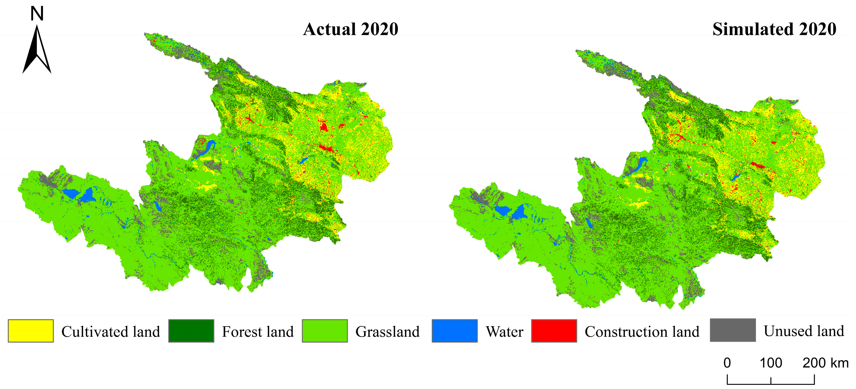
The Gansu–Qinghai contiguous region of the upper Yellow River is predominantly characterized by ecological landscapes such as grassland and forest land, which collectively form the main ecological spaces in the region. As an illustration, the 2020 data reveal that forest land and grassland, which constitute the ecological space, cover 80.21% of the area. In contrast, cultivated land, which represents the production space, accounted for 9.75%, while construction land, denoting the living space, accounted for 1.19% (Figure 3). Among these, grasslands are the most extensive, whereas construction lands are the least widespread, with their presence mainly confined to the areas surrounding the main channel and tributaries of the Yellow River (

Table 6. Land use type area during 1980–2020 and land use simulation area during 2030–2040 under three scenarios (km²).

	1980	2020	BAU2030	CLP2030	EP2030	BAU2040	CLP2040	EP2040
Cultivated Land	23,042.95	22,830.28	22,512.55	23,145.54	22,512.55	22,206.56	23,754.52	22,206.56
Forest Land	27,296.95	27,038.16	27,184.46	27,184.46	27,225.46	27,246.46	26,450.47	27,245.46
Grassland	162,294.68	160,730.47	160,065.80	160,065.80	160,783.78	159,454.81	159,453.81	161,376.77
Water	4137.99	4393.62	4459.91	4459.91	4381.91	4535.91	4535.91	4427.91
Construction Land	1629.00	2795.85	3626.93	2960.94	2954.94	3784.92	3083.94	3110.94
Unused Land	15,695.97	16,301.77	16,243.68	16,276.67	16,234.68	16,864.66	16,814.66	15,725.69

).

By inputting neighborhood factors, cost transfer matrices, and land use demand data into the FLUS model, we estimated land use conditions for the three scenarios in 2030 and 2040. According to our estimations, the pace of land use change in 2020 was not as rapid as actually observed, particularly in the case of construction land, which indicates a slower urbanization process than expected. Nonetheless, there is a projection for a significant expansion of construction land, primarily driven by human activities and the growth of urban transportation networks. Under the BAU scenario, there has been a notable increase in construction land, often at the expense of encroaching on adjacent cultivated land and forest land. This trend raises concerns about the potential for urbanization to inflict considerable damage on valuable agricultural and grassland. As urban areas expand, we observe a persistent decline in the spatial distribution of cultivated land. Conversely, in the CLP scenario, which enforces stringent cultivated land protection policies, the necessity to meet food demands curtails the transformation of grassland into cultivated land. This scenario underscores the importance of balancing land use to maintain food security. The vegetation landscape shows significant regional variations across different scenarios. The EP scenario, in particular, indicates a progressive increase in grassland coverage over time, which enhances ecological land use and yields greater ecological benefits. However, the BAU and CLP scenarios demonstrate a considerable decrease in grasslands, especially in proximity to urban centers. Across all examined scenarios, grasslands serve as transitional areas, often changing between different land use types, as depicted in Figure 4. This intermediary role of grassland highlights its importance in land use planning and the need for careful management to ensure sustainable transitions between various land uses (Figure 4).

3.1.2. Land Use Change Analysis during 1980 to 2040

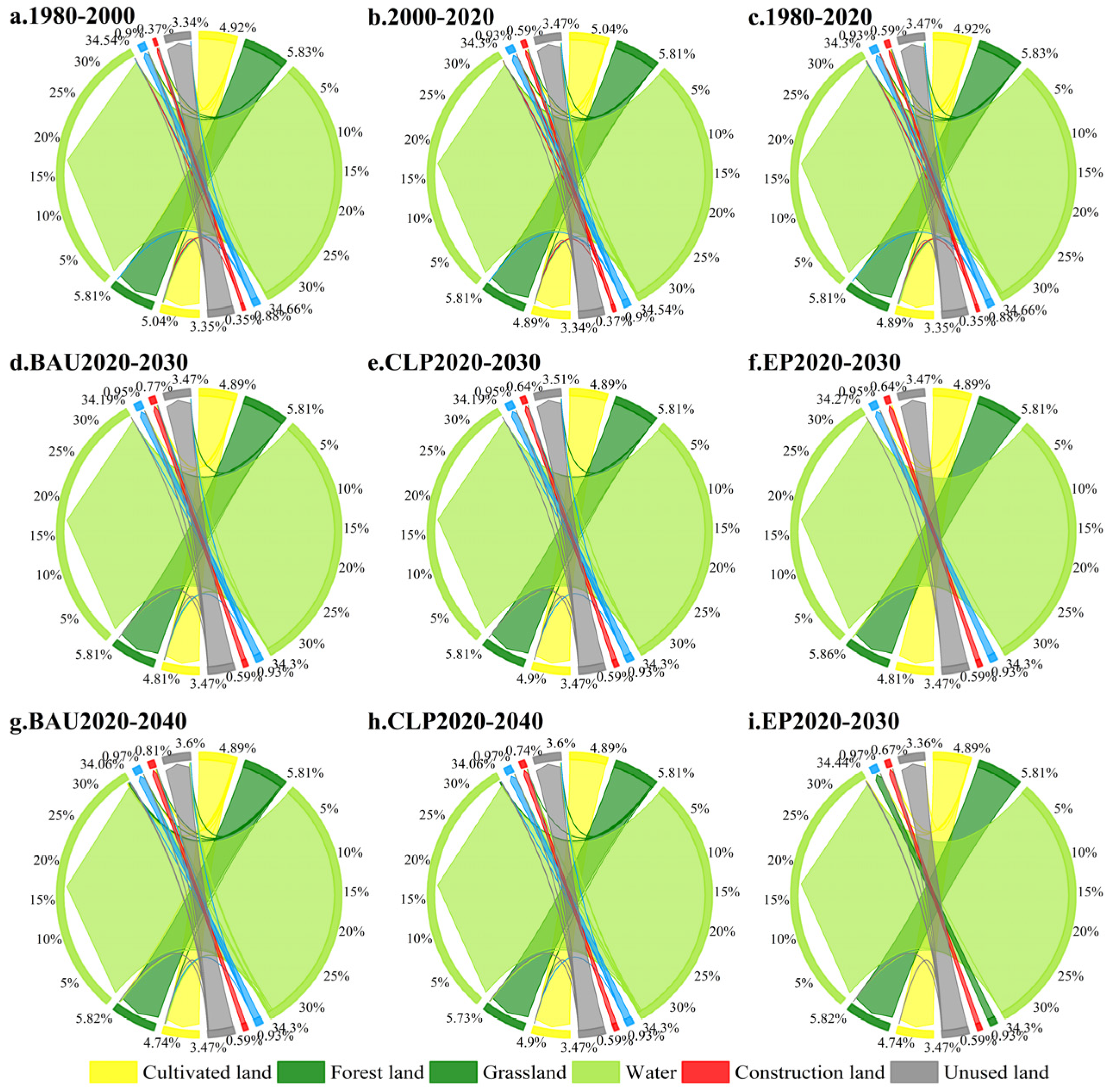
In analyzing the chordal map of land use transfer from 1980 to 2040, we aim to reveal the dynamic change process of land use types in the study area, especially the trend of forest land, grassland, cultivated land and construction land. The string diagram of the land use transfer shows details of the land use conversion from 1980 to 2040 (Figure 5). Over the past four decades, the predominant shift in land use within the study area has seen a reduction in the expanse of forest land and grassland serving as ecological spaces, a decrease in the area of cultivated land functioning as production spaces, and an expansion of developed areas for habitation. Within this context, the expansion of construction land and the reduction in grassland have proceeded at a stable rate, whereas the trends for cultivated land and forest land have been more variable. Between 1980 and 2000, land use transitions were minor, both in terms of direction and area affected, resulting in a stable land use structure; however, from 2000 to 2020, with a significant shift of 2726.6 km², the degree of conversion intensified, and human activity became more pronounced during this period.

Over the four decades, grasslands, serving as intermediary and adjacent land types, experienced frequent transitions. The area of grassland diminished by 1676.7 km², a 0.38% decrease, while forest land saw a reduction of 78.5 km², which is a 0.02% decrease. The primary conversions of forest land and grassland ecological lands were to cultivated land. Intense demand for agricultural land has driven the transformation from cultivated land to forest land and grassland. The shrinkage of forest land and grassland areas not only compromises local habitat quality, but also impacts water conservation capabilities, carbon sequestration, and more. Factors such as agricultural intensification and the abandonment of cultivated land have led to a reduction in cultivated land area by 138.9 km² (0.03%), with the majority being converted into grassland and construction land.

From 2020 to 2040, it is anticipated that the structure of land use will undergo significant transformations. Among the three scenarios considered, variations in grassland are the most pronounced, which is attributed to its status as the most predominant ecosystem in the region. The scenarios differ in terms of the types of land being converted: The BAU scenario is marked by a notable conversion of grassland. The CLP scenario also sees grassland being predominantly converted. The EP scenario is distinguished by conversions of cultivated land and unused land. In the CLP scenario, arable land is the only category that experiences growth, with an increase of approximately 924.24 km² (0.01%), while it decreases in the BAU and EP scenarios by 0.15%. Under robust ecological protection measures, forest land and grassland ecological areas are expanded in the EP scenario, by about 207.3 km² (0.01%) and 646.3 km² (0.14%), respectively. Water resources trends are consistent across scenarios, with increases observed in both the BAU and CLP scenarios, whereas the EP scenario shows a decrease. The trend in the expansion of construction land is also consistent across scenarios, with the most substantial increase occurring in the BAU scenario (BAU, 0.22%; CLP, 0.15%; EP, 0.08%).

3.2. Habitat Quality and Spatial and Temporal Variation

3.2.1. Spatial and Temporal Evolution of Habitat Quality (1980–2040)

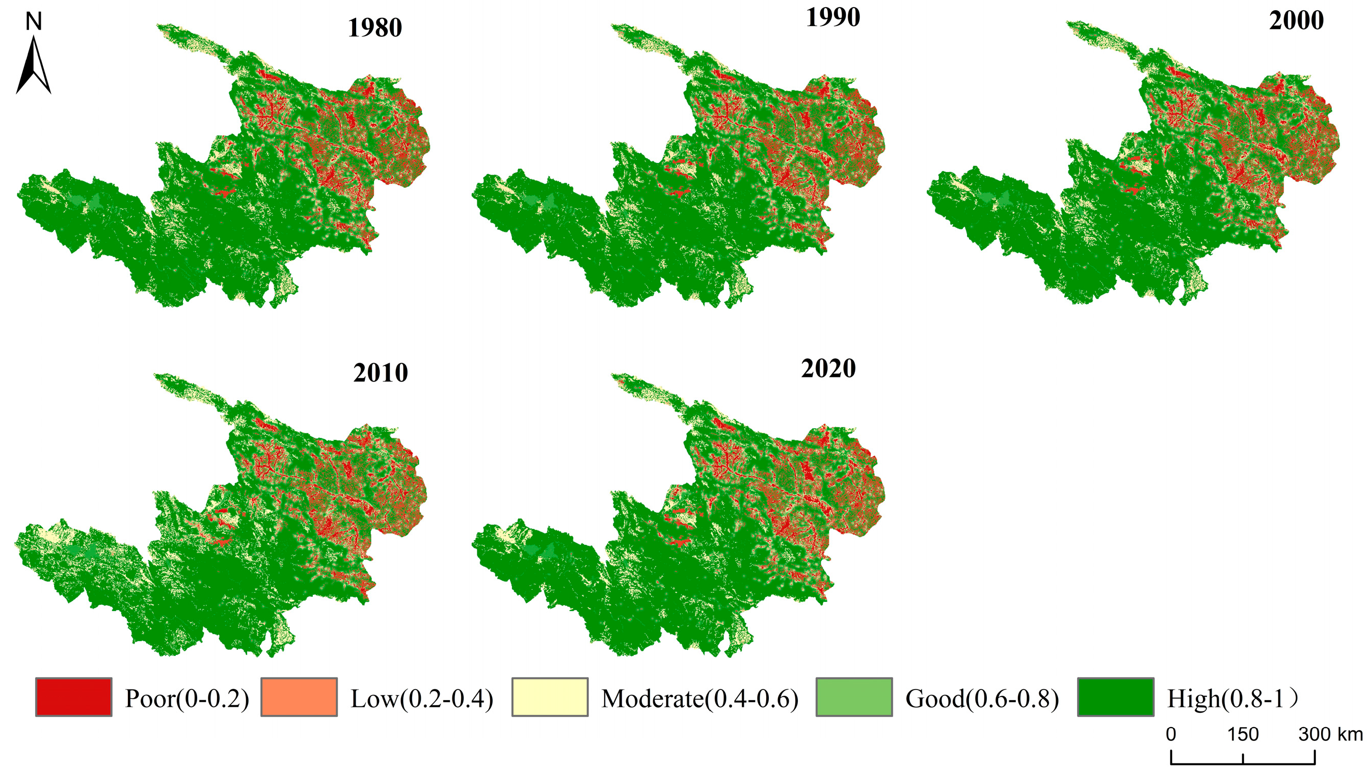
Values for habitat quality range from 0 (non-habitat quality) to 1 (maximum suitability habitat quality) (Figure 6). In this study, habitat quality was divided into five equally spaced classes, which are poor (0–0.2), low (0.2–0–0.4), moderate (0.4–0.6), good (0.6–0.8) and high (0.8–1.0)

To quantify and analyze trends in habitat quality between 1980 and 2020, we here collect and analyze data to understand how habitat quality has changed over time, and whether these changes are significant. The mean habitat quality values in 1980, 1990, 2000, 2010 and 2020 were 0.8543, 0.8538, 0.8516, 0.8353 and 0.8449. Overall, habitat quality was at a high level over the 40 years, and showed a downward and then upward trend. Areas with lower habitat quality expanded, while areas with higher habitat quality decreased. The predominant ecological types in the study area are forest land and grassland. Over time, as human activity has increased, the quality of habitat has decreased. Spatially, the habitat quality in the central region is lower than in the surrounding areas, with lower quality in the east and higher quality in the west, which is mainly influenced by land type and climate.

To study how changes in land use types affect habitat quality, we particularly focused on the impacts of anthropogenic land use changes on ecosystem structure and function. While the predicted quantity and spatial distribution of forest land and grassland ecological lands varied under the three scenarios, these lands were generally found in areas of high habitat quality. In contrast, construction land consistently appeared in areas of low habitat quality. By examining the spatial patterns of land use alongside habitat quality in the study area, we observe a strong correlation between the expansion of construction land and the presence of low-habitat-quality areas, as exemplified by the development of the Lanzhou New Area and its corresponding low habitat quality index. Similarly, regions designated as ecological spaces often coincided with areas of high habitat quality. Notably, the Yushu Tibetan Autonomous Prefecture, located at the source of three major rivers on the Qinghai–Tibet Plateau, suffered severe degradation and a significant decline in habitat quality between 2000 and 2020. Given its critical ecological importance, the area requires urgent restoration efforts.

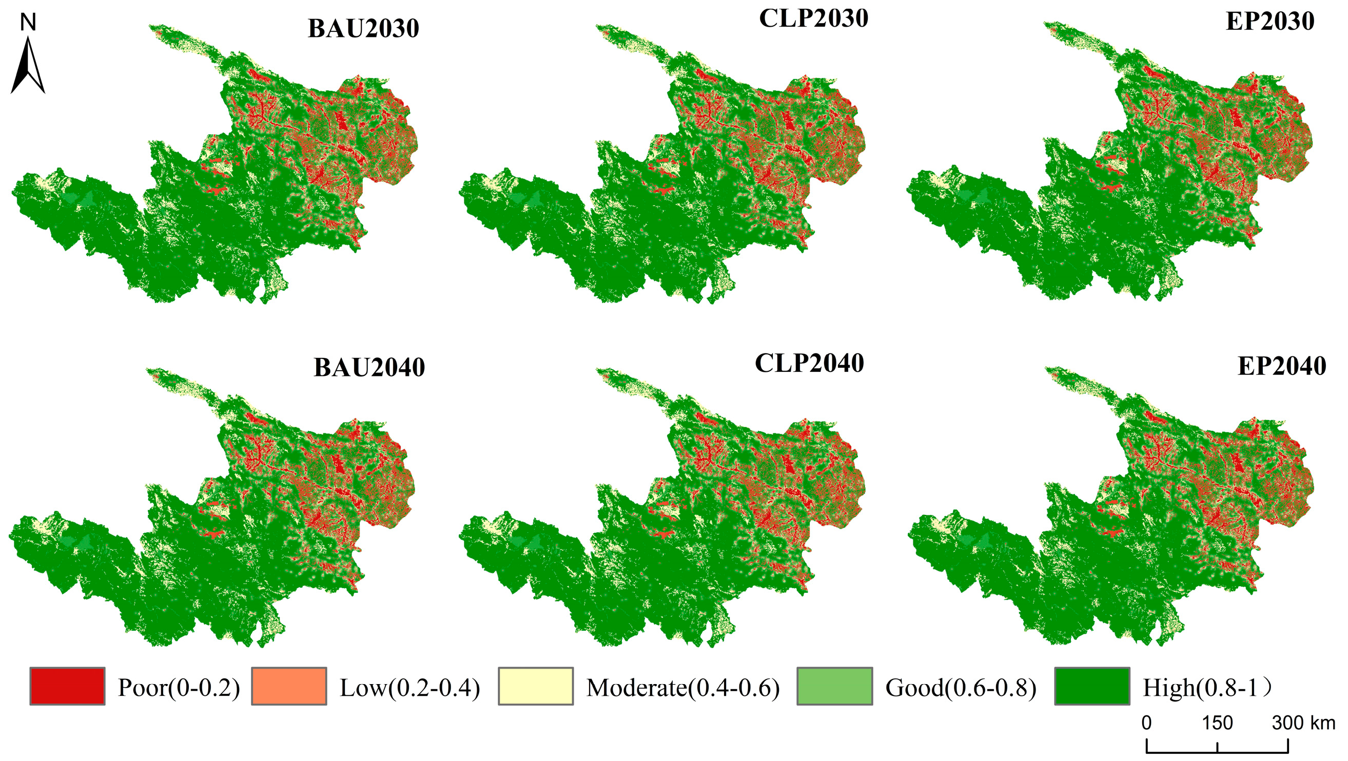
To analyze the impacts of different policies or management strategies, we compared the predictions under three different scenarios: BAU, CLP and EP (Figure 7). The headquarters index, serving as a measure of ecosystem services, indicates the overall ecological condition of the study area. By 2030, the estimated average habitat quality values in the upper Yellow River are projected to be 0.8405, 0.8419 and 0.8434, respectively. For 2040, the projections are 0.8398, 0.8388 and 0.8450, respectively. Throughout the forecast period and under the three scenarios, the EP scenario is expected to maintain the highest habitat quality value, followed by the CLP scenario, with the BAU scenario yielding the lowest values. Our projections suggest a decline in habitat quality across all scenarios, primarily attributed to extensive land requisition for regional development to accommodate urbanization. Taking 2030 as an example, the BAU, CLP, and EP scenarios are predicted to decrease by 0.0029 (0.34%), 0.0015 (0.18%), and 0.0001, respectively. The EP protocol, despite the anticipated greatest reduction in habitat quality, represents an idealized outcome. The EP scenario shows a pronounced reduction, especially in the Huangnan and Guoluo Tibetan Autonomous Prefecture. For instance, the BAU scenario predicts the most significant degradation by 2030, while the EP scenario projects the least impact. Within the context, the areas of degradation under the CLP scenario are primarily located in Gande and Zeku counties. Conversely, the EP scenario’s degradation is mainly expected along the borders Dali and Machin counties of Qinghai Province.

It is anticipated that the extremities of habitat quality values representing high-quality areas and areas of differentiation will exhibit a trend of contraction in optimal areas and expansion in differentiated areas. The intermediate habitat quality values include both higher- and lower-quality areas, with higher-quality areas expected to increase and differentiated areas expected to decrease (Figure 8). Compared with 2020, the extent of high-quality areas is projected to decrease by varying degrees by 2030, with the EP scenario demonstrating the most favorable outcome, showing the least reduction of 59 km². The size of the high-quality regions is expected to increase in different ranges, with the BAU scenario outperforming the others, leading to the most significant increase in high-quality area to 505.99 km². In terms of moderate-quality areas, the CLP scenario is predicted to perform the best, showing an increase, while the BAU scenario is expected to perform the worst, with a decrease. Low-quality regions are expected to experience varying degrees of reduction, with the BAU scenario again performing the best, minimizing the decrease to 284.99 km². Across different ranges, the EP scenario is anticipated to perform the best, with the smallest increase of 100 km² in low-quality areas. Overall, the EP scenario is expected to yield the most favorable results in terms of habitat quality performance.

3.2.2. Analysis of Spatial and Temporal Variation in Habitat Quality (1980–2040)

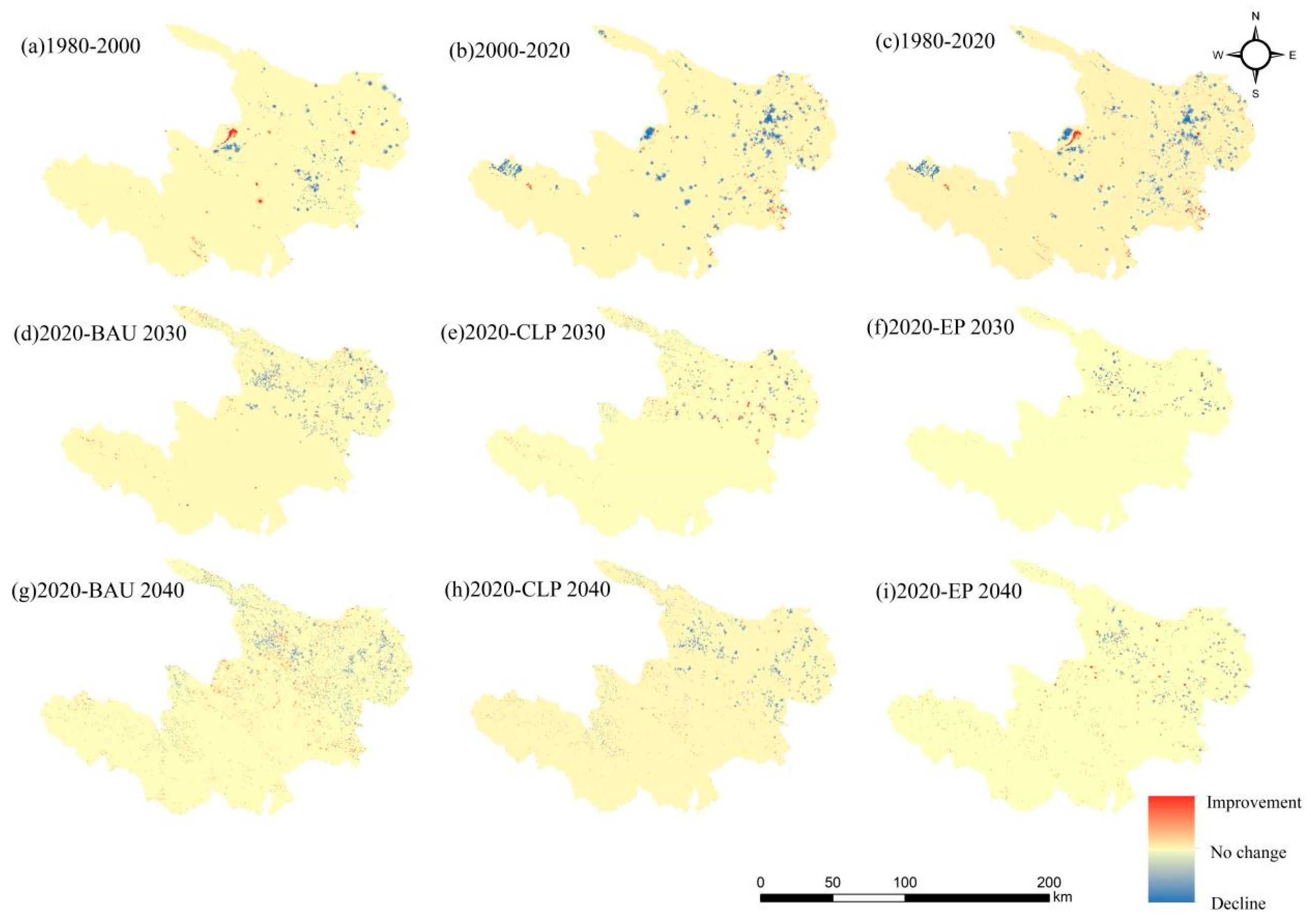
Habitat quality changes were categorized into three levels: decline (−4 to −0.0001), no change (−0.0001 to 0), and improvement (0 to 4). Land use alterations exert a notable influence on habitat quality, as do transportation factors. Notably, the areas where habitat quality has degraded align closely with regions affected by transportation factors. This degradation is largely attributable to the substantial disruption caused by these factors. When comparing the periods 1980–2020 and 2000–2020, it is evident that habitat degradation is consistently associated with the presence of transportation infrastructure. Trends in habitat quality were similar under the three scenarios, but the spatial distribution was significantly different. For instance, projections for 2030 suggest that under the BAU scenario, there will be a primary decline in habitat quality, especially in the northern part. Conversely, the CLP scenario predicts both a decrease and an increase in habitat quality. However, the EP scenario presents a reduction in habitat quality in both the areas previously experiencing decline and those showing an increase. Despite these changes, there is no significant decrease in the average habitat quality in 2030 when compared to 2020. Particularly, the EP scenario effectively curtails the growth of living and production spaces, reverses the trend of ecological degradation, and promotes the diversity of ecological lands, signaling a modest improvement in habitat quality. Therefore, the EP approach is the preferred strategy for preserving high-quality habitats. By 2040, the extent of change is expected to be more pronounced than in 2030 (Figure 9).

4. Discussion

4.1. Analysis of the Factors Influencing the Habitat Quality

The quality of habitats serves as a crucial metric for assessing the ecological condition of a region [40]. Forecasting the trajectory of habitat quality is essential as it equips policymakers with a scientific foundation for crafting strategies aimed at habitat conservation and the judicious distribution of natural resources. Both natural elements and anthropogenic factors shape habitat quality, with human activities inflicting considerable detrimental effects on terrestrial environments [41]. These effects manifest as habitat destruction, biodiversity diminishment, vegetation impairment, and overall ecological degradation. In the Gansu–Qinghai contiguous region of the upper Yellow River, these include deforestation, the overgrazing of grasslands, and mineral exploitation, and they will destroy the original ecosystem structure and affect biodiversity, which may lead to a decrease in vegetation cover and a deterioration of the ecological environment. The disturbance and destruction of the ecosystem by human activities can lead to the degradation of the whole ecosystem. In the Gansu–Qinghai contiguous region of the upper Yellow River, this may lead to problems such as a decline in water-holding capacity and increased soil erosion. Presently, numerous nations grapple with grave environmental issues stemming from human-driven processes such as industrialization, agriculture, and urban expansion. In the study area, areas designated for ecological rehabilitation typically coincide with terrains characterized by gentler slopes and lower altitudes. The reasons for this are twofold: such topographies are more conducive to vegetation proliferation and concurrently less accommodating of human endeavors. These observations are corroborated by findings from additional research. In the Gansu–Qinghai contiguous region of the upper Yellow River, areas with gentler slopes may be more suitable for vegetation restoration because they are less prone to soil erosion and can provide better growing conditions. In the Gansu–Qinghai contiguous region of the upper Yellow River, the lower-elevation areas are usually warmer and more favorable for plant growth, but may also face pressure from human activities such as overgrazing and agricultural development. Higher-altitude areas may face harsher climatic conditions, making vegetation recovery more difficult [42].

4.2. The Impact of the Policy on the Habitat Quality

Land use resource allocation and management policies significantly influence land use changes [43]. On 30 November 2017, Gansu Province promulgated the Regulations on the Management of Gansu Qilian Mountain National Nature Reserve, aimed primarily at bolstering the safeguarding and stewardship of water conservation forest Lands within the Qilian Mountain National Nature Reserve in Gansu. The implementation of the regulations has led to an increase in vegetation cover in the region, a reduction in soil erosion, and an increase in the capacity of water sources to contain water, thus indirectly improving the quality and quantity of water in the Gansu–Qinghai contiguous region of the upper Yellow River. The enactment of such conservation initiatives has markedly enhanced the environmental quality of the Gansu–Qinghai contiguous region of the upper Yellow River. The Gannan Tibetan Autonomous Prefecture, situated on the northeastern fringe of the Qinghai–Tibet Plateau and the western expanse of the Loess Plateau, holds undeniable significance. Gannan Tibetan Autonomous Prefecture is an important ecological barrier in the upper reaches of the Yellow River, and the deterioration of its ecological environment will affect the ecological stability of the entire basin. Over the past four decades, local habitats have experienced ongoing degradation, with the Cooperative City in the Gannan Tibetan Autonomous Prefecture being a notable area in need of ecological restoration. In August 2012, the State Council designated the Lanzhou New Area as a national-level new district. The noticeable decline in the habitat quality index of the Lanzhou New Area between 2010 and 2020 is evidently associated with its development. The industrial development of Lanzhou New Area may bring the discharge of wastewater, exhaust gas and other pollutants, which may affect the water quality and ecological environment of the upper reaches of the Yellow River through rivers and the atmosphere [44].

4.3. Ecosystem Sustainable Management Recommendations and Strategies

Based on the habitat quality prediction model for the Gansu–Qinghai contiguous region of the upper Yellow River under various scenarios, this study indicates that habitat quality is expected to improve with the adoption of land use practices that emphasize farmland protection and environmental conservation [45]. To enhance future habitat quality and reinforce ecosystem functions in the Gansu–Qinghai contiguous region of the upper Yellow River, the following recommendations are put forward: Rigorously enforce the ecological red line policy and associated environmental regulations, giving particular attention to critical buffer areas such as the Gannan Tibetan Autonomous Prefecture, as well as ecologically sensitive and delicate regions. Promote environmental rehabilitation and improve the distribution of land resources. Safeguard the current ecological areas without diminishing their extent, and refine the spatial arrangement of different habitat types, including forest lands, pastures, and water bodies. In the process of developing land use plans at all levels, it is crucial to manage the total area allocated for development judiciously to minimize reliance on newly developed land [46].

4.4. Function, Interpretation, and Limitations of the Model

The FLUS model addresses some of the limitations of traditional land use simulation methods and offers an effective approach for forecasting land use changes. Nevertheless, the model is not without its uncertainties [47]. One of the constraints of the FLUS model is the assumption that transfer rules remain constant, which may not align with reality, as shifts in development policies can alter existing conditions. Additionally, the model relies on precise predictions of future land use changes, which inherently contain uncertainties. Consequently, the scenario outcomes from this study should be used with caution by managers and policymakers, serving as a reference rather than definitive predictions. Moreover, the difficulty in quantifying policy factors means that influences such as protected areas and ecological function areas are not fully accounted for in the simulation of land use structure, which may impact the accuracy of the simulations. The InVSET habitat quality module used for assessing habitat quality does offer advantages over other ecological assessment tools. However, it also has its shortcomings, particularly in the assessment of habitat quality. For instance, the parameters for habitat threat and sensitivity factors are derived from expert knowledge, which introduces a level of subjectivity. Although hierarchical analysis methods were employed to mitigate potential biases and enhance objectivity, future improvements to the model are necessary to further refine its accuracy and reliability. We recognize that there may be potential limitations or conflicting results between different studies in the academic field. For example, Yohannes et al. [47,48] explored habitat quality change in the Beressa watershed of the Blue Nile basin in the Ethiopian highlands. It was influenced by specific cultural contexts and geographical constraints, which prevented the results from being broadly applicable to the present study.

Although three scenarios were considered in this study, the CLP-EP scenario is closer to possible future urbanization trends. It is recommended that these socio-economic scenarios be included in the future so as to better understand the different changes in habitat quality under different future development scenarios. This will contribute to a better understanding of the potential impacts of climate change and socio-economic factors on habitat quality. In addition, the projection of the future situation remains theoretical, lacking a discussion of practical problems and their causes.

5. Conclusions

This study has evaluated habitat quality from 1980 to the present, and provided an in-depth analysis of its spatial and temporal evolution characteristics as well as trends in habitat quality in 2030 and 2040 under three scenarios. The main conclusions are as follows.

Overall, the habitat quality was at a high level within the 40 years, and showed a downward and then upward trend. Areas with lower habitat quality expanded and areas with higher habitat quality decreased. On the spatial scale, the habitat quality in the central region is lower than in the surrounding areas, and is lower in the east and higher in the west, mainly influenced by land type and climate.

Habitat quality is projected to be highest under the ecological protection (EP) scenario, with the farmland protection scenario ranking second, and the natural situation scenario yielding the lowest values. The EP scenario is particularly effective at curbing the expansion of residential and industrial areas, reversing the trends of ecological degradation, and promoting the diversity of ecological land. It emerges as the preferred strategy for sustaining high-quality habitats. The reduction in habitat quality under the EP scenario is especially pronounced in the Huangnan and the Guoluo Tibetan Autonomous Prefecture.

It is anticipated that the extreme values of the habitat quality index—representing high-quality and poor-quality areas—will exhibit a trend towards a reduction in optimal habitats and an expansion in areas of disparity. Areas with intermediate habitat quality values are likely to experience an increase in high-quality habitats and a decrease in disparate habitats. Although the BAU, CLP, and EP scenarios predict similar general trends in habitat quality changes, their geographical distribution will differ markedly. By the year 2030, under the BAU scenario, a predominant decline in habitat quality is expected, with a significant concentration of this decline. In the CLP scenario, there will be both a decrease and an increase in habitat quality areas. In contrast, the EP scenario forecasts a decline in habitat quality across both diminishing and improving regions.

Specifically, while there are variances in the projected quantity and spatial distribution of forest land and grassland ecological land uses across the three scenarios, they are all anticipated to occur within areas of high habitat quality. In contrast, urban development land consistently falls within areas of low habitat quality. A comparison of the spatial patterns of land use and habitat quality in the study area reveals a high degree of overlap between the expansion areas of urban development and the regions of low habitat quality. This can be seen, for example, in the correlation between the habitat quality index’s development and the limited urban expansion in the Lanzhou New Area. Similarly, there is a correspondence between the areas designated for ecological spatial distribution and the areas of high habitat quality.

References

1. Wang, H.; Hu, Y.; Yan, H.; Liang, Y.; Guo, X.; Ye, J. Trade-off among grain production, animal husbandry production, and habitat quality based on future scenario simulations in Xilinhot. Sci. Total Environ. 2022, 817, 153015. [Google Scholar] [CrossRef] [PubMed]
2. Angel, S.; Parent, J.; Civco, D.L.; Blei, A.; Potere, D. The dimensions of global urban expansion: Estimates and projections for all countries, 2000–2050. Prog. Plann. 2011, 75, 53–107. [Google Scholar] [CrossRef]
3. Seto, K.C.; Fragkias, M.; Güneralp, B.; Reilly, M.K. A meta-analysis of global urban land expansion. PLoS ONE 2021, 6, e23777. [Google Scholar] [CrossRef] [PubMed]
4. Myers, N.; Mittermeier, R.A.; Mittermeier, C.G.; Da Fonseca, G.A.; Kent, J. Biodiversity hotspots for conservation priorities. Nature 2000, 403, 853–858. [Google Scholar] [CrossRef] [PubMed]
5. White, R.; Engelen, G. Cellular automata and fractal urban form: A cellular modelling approach to the evolution of urban land-use patterns. Environ. Plan. A 1993, 25, 1175–1199. [Google Scholar] [CrossRef]
6. Song, Y.; Xue, D.; Dai, L.; Wang, P.; Huang, X.; Xia, S. Land cover change and eco-environmental quality response of different geomorphic units on the Chinese Loess Plateau. J. Arid Land 2020, 12, 29–43. [Google Scholar] [CrossRef]
7. Liang, X.; Liu, X.; Li, X.; Chen, Y.; Tian, H.; Yao, Y. Delineating multi-scenario urban growth boundaries with a CA-based FLUS model and morphological method. Landscape Urban Plan. 2018, 177, 47–63. [Google Scholar] [CrossRef]
8. Zhang, T.; Chen, Y. The effects of landscape change on habitat quality in arid desert areas based on future scenarios: Tarim River Basin as a case study. Front. Plant Sci. 2022, 13, 1031859. [Google Scholar] [CrossRef] [PubMed]
9. Wei, Q.; Abudureheman, M.; Halike, A.; Yao, K.; Yao, L.; Tang, H.; Tuheti, B. Temporal and spatial variation analysis of habitat quality on the PLUS-InVEST model for Ebinur Lake Basin, China. Ecol. Indic. 2022, 145, 109632. [Google Scholar] [CrossRef]
10. Yang, J.; Xie, B.; Zhang, D.; Mak-Mensah, E.; Pei, T. Habitat quality assessment and multi-scenario prediction of the Gansu-Qinghai section of the Yellow River Basin based on the FLUS-InVEST model. Front. Ecol. Evol. 2023, 11, 1228558. [Google Scholar] [CrossRef]
11. Tang, F.; Fu, M.; Wang, L.; Zhang, P. Land-use change in Changli County, China: Predicting its spatio-temporal evolution in habitat quality. Ecol. Indic. 2020, 117, 106719. [Google Scholar] [CrossRef]
12. Daily, G.C.; Polasky, S.; Goldstein, J.; Kareiva, P.M.; Mooney, H.A.; Pejchar, L.; Ricketts, T.H.; Salzman, J.; Shallenberger, R. Ecosystem services in decision making: Time to deliver. Front. Ecol. Environ. 2009, 7, 21–28. [Google Scholar] [CrossRef]
13. Wang, F. The use of artificial neural networks in a geographical information system for agricultural land-suitability assessment. Environ. Plann. A 1994, 26, 265–284. [Google Scholar] [CrossRef]
14. Liang, X.; Guan, Q.; Clarke, K.C.; Liu, S.; Wang, B.; Yao, Y. Understanding the drivers of sustainable land expansion using a patch-generating land use simulation (PLUS) model: A case study in Wuhan, China. Comput. Environ. Urban 2021, 85, 101569. [Google Scholar] [CrossRef]
15. Fu, F.; Deng, S.; Wu, D.; Liu, W.; Bai, Z. Research on the spatiotemporal evolution of land use landscape pattern in a county area based on CA-Markov model. Sustain. Cities Soc. 2022, 80, 103760. [Google Scholar] [CrossRef]
16. Nematollahi, S.; Fakheran, S.; Kienast, F.; Jafari, A. Application of InVEST habitat quality module in spatially vulnerability assessment of natural habitats (case study: Chaharmahal and Bakhtiari province, Iran). Environ. Monit. Assess. 2020, 192, 487. [Google Scholar] [CrossRef] [PubMed]
17. Bai, L.; Xiu, C.; Feng, X.; Liu, D. Influence of urbanization on regional habitat quality: A case study of Changchun City. Habitat. Int. 2019, 93, 102042. [Google Scholar] [CrossRef]
18. Guo, H.; Cai, Y.; Yang, Z.; Zhu, Z.; Ouyang, Y. Dynamic simulation of coastal wetlands for Guangdong-Hong Kong-Macao Greater Bay area based on multi-temporal Landsat images and FLUS model. Ecol. Indic. 2021, 125, 107559. [Google Scholar] [CrossRef]
19. Li, F.; Wang, L.; Chen, Z.; Clarke, K.C.; Li, M.; Jiang, P. Extending the SLEUTH model to integrate habitat quality into urban growth simulation. J. Environ. Manag. 2018, 217, 486–498. [Google Scholar] [CrossRef]
20. Zhang, Z.; Hu, B.; Jiang, W.; Qiu, H. Identification and scenario prediction of degree of wetland damage in Guangxi based on the CA-Markov model. Ecol. Indic. 2021, 127, 107764. [Google Scholar] [CrossRef]
21. Chen, X.; He, X.; Wang, S. Simulated validation and prediction of land use under multiple scenarios in Daxing District, Beijing, China, Based on GeoSOS-FLUS Model. Sustainability 2022, 14, 11428. [Google Scholar] [CrossRef]
22. Li, Y.; Liu, Z.; Li, S.; Li, X. Multi-scenario simulation analysis of land use and carbon storage changes in changchun city based on FLUS and InVEST model. Land 2022, 11, 647. [Google Scholar] [CrossRef]
23. Ding, Q.; Chen, Y.; Bu, L.; Ye, Y. Multi-Scenario Analysis of Habitat Quality in the Yellow River Delta by Coupling FLUS with InVEST Model. Int. J. Environ. Res. Public Health 2021, 18, 2389. [Google Scholar] [CrossRef] [PubMed]
24. Zhang, C.; Wang, P.; Xiong, P.; Li, C.; Quan, B. Spatial pattern simulation of land use based on FLUS model under ecological protection: A case study of Hengyang City. Sustainability 2021, 13, 10458. [Google Scholar] [CrossRef]
25. Yang, Y. Evolution of habitat quality and association with land-use changes in mountainous areas: A case study of the Taihang Mountains in Hebei Province, China. Ecol. Indic. 2021, 129, 107967. [Google Scholar] [CrossRef]
26. Falcucci, A.; Maiorano, L.; Boitani, L. Changes in land-use/land-cover patterns in Italy and their implications for biodiversity conservation. Landscape Ecol. 2007, 22, 617–631. [Google Scholar] [CrossRef]
27. Zhang, Y.; Lu, X.; Liu, B.; Wu, D.; Fu, G.; Zhao, Y.; Sun, P. Spatial relationships between ecosystem services and socioecological drivers across a large-scale region: A case study in the Yellow River Basin. Sci. Total Environ. 2021, 766, 142480. [Google Scholar] [CrossRef] [PubMed]
28. Liu, X.; Liang, X.; Li, X.; Xu, X.; Ou, J.; Chen, Y.; Li, S.; Wang, S.; Pei, F. A future land use simulation model (FLUS) for simulating multiple land use scenarios by coupling human and natural effects. Landscape Urban Plan. 2017, 168, 94–116. [Google Scholar] [CrossRef]
29. Nelson, E.; Mendoza, G.; Regetz, J.; Polasky, S.; Tallis, H.; Cameron, D.; Chan, K.M.A.; Daily, G.C.; Goldstein, J.; Kareiva, P.M.; et al. Modeling multiple ecosystem services, biodiversity conservation, commodity production, and tradeoffs at landscape scales. Front. Ecol. Environ. 2009, 7, 4–11. [Google Scholar] [CrossRef]
30. Wu, L.; Sun, C.; Fan, F. Estimating the characteristic spatiotemporal variation in habitat quality using the invest model—A case study from Guangdong–Hong Kong–Macao Greater Bay Area. Remote Sens. 2021, 13, 1008. [Google Scholar] [CrossRef]
31. Ye, H.; Song, Y.; Xue, D. Multi-scenario simulation of land use and habitat quality in the Guanzhong plain urban agglomeration, China. Int. J. Environ. Res. Public Health 2022, 19, 8703. [Google Scholar] [CrossRef] [PubMed]
32. Liu, X.; Wei, M.; Li, Z.; Zeng, J. Multi-scenario simulation of urban growth boundaries with an ESP-FLUS model: A case study of the Min Delta region, China. Ecol. Indic. 2022, 135, 108538. [Google Scholar] [CrossRef]
33. Zhang, X.; Song, W.; Lang, Y.; Feng, X.; Yuan, Q.; Wang, J. Land use changes in the coastal zone of China’s Hebei Province and the corresponding impacts on habitat quality. Land Use Policy 2020, 99, 104957. [Google Scholar] [CrossRef]
34. Gomes, E.; Inácio, M.; Bogdzevič, K.; Kalinauskas, M.; Karnauskaitė, D.; Pereira, P. Future scenarios impact on land use change and habitat quality in Lithuania. Environ. Res. 2021, 197, 111101. [Google Scholar] [CrossRef] [PubMed]
35. Sallustio, L.; De Toni, A.; Strollo, A.; Di Febbraro, M.; Gissi, E.; Casella, L.; Marchetti, M. Assessing habitat quality in relation to the spatial distribution of protected areas in Italy. J. Environ. Manag. 2017, 201, 129–137. [Google Scholar] [CrossRef] [PubMed]
36. Jayanthi, M.; Duraisamy, M.; Thirumurthy, S.; Samynathan, M.; Muralidhar, M. Dynamics of land-use changes and their future trends using spatial analysis and the CA-Markov model—A case-study with a special emphasis on aquaculture development in India. Land Degrad. Dev. 2021, 32, 2563–2579. [Google Scholar] [CrossRef]
37. Tang, F.; Wang, L.; Guo, Y.; Fu, M.; Huang, N.; Duan, W.; Luo, M.; Zhang, J.; Li, W.; Song, W. Spatio-temporal variation and coupling coordination relationship between urbanisation and habitat quality in the Grand Canal, China. Land Use Policy 2022, 117, 106119. [Google Scholar] [CrossRef]
38. Upadhaya, S.; Dwivedi, P. Conversion of forestlands to blueberries: Assessing implications for habitat quality in Alabaha river watershed in Southeastern Georgia, United States. Land Use Policy 2019, 89, 104229. [Google Scholar] [CrossRef]
39. Terrado, M.; Sabater, S.; Chaplin-Kramer, B.; Mandle, L.; Ziv, G.; Acuña, V. Model development for the assessment of terrestrial and aquatic habitat quality in conservation planning. Sci. Total Environ. 2016, 540, 63–70. [Google Scholar] [CrossRef]
40. Liu, M.; Zhang, Z.; Sun, J.; Li, Y.; Liu, Y.; Berihun, M.L.; Xu, M.; Tsunekawa, A.; Chen, Y. Restoration efficiency of short-term grazing exclusion is the highest at the stage shifting from light to moderate degradation at Zoige, Tibetan Plateau. Ecol. Indic. 2020, 114, 106323. [Google Scholar] [CrossRef]
41. Ren, J.; Zhao, X.Y.; Xu, X.C.; Ma, P.Y.; Du, Y.X. Spatial-temporal evolution, tradeoffs and synergies of ecosystem services in the middle Yellow River. J. Earth Environ. 2022, 13, 477–490. [Google Scholar]
42. Liu, Z.F.; Tang, L.N.; Qiu, Q.Y.; Xiao, L.; Xu, T.; Yang, L. Temporal and spatial changes in habitat quality based on land-use change in Fujian Province. Acta Ecol. Sin. 2017, 37, 4538–4548. [Google Scholar]
43. Jiang, L.; Wang, Z.; Zuo, Q.; Du, H. Simulating the impact of land use change on ecosystem services in agricultural production areas with multiple scenarios considering ecosystem service richness. J. Clean. Prod. 2023, 397, 136485. [Google Scholar] [CrossRef]
44. Güneralp, B.; Seto, K.C. Futures of global urban expansion: Uncertainties and implications for biodiversity conservation. Environ. Res. Lett. 2013, 8, 014025. [Google Scholar] [CrossRef]
45. Seto, K.C.; Güneralp, B.; Hutyra, L.R. Global forecasts of urban expansion to 2030 and direct impacts on biodiversity and carbon pools. Proc. Natl. Acad. Sci. USA 2012, 109, 16083–16088. [Google Scholar] [CrossRef]
46. Zhang, X.; Zhou, J.; Li, G.; Chen, C.; Li, M.; Luo, J. Spatial pattern reconstruction of regional habitat quality based on the simulation of land use changes from 1975 to 2010. J. Geogr. Scis. 2020, 30, 601–620. [Google Scholar] [CrossRef]
47. Collinge, S.K. Ecological consequences of habitat fragmentation: Implications for landscape architecture and planning. Landscape Urban Plan. 1996, 36, 59–77. [Google Scholar] [CrossRef]
48. Yohannes, H.; Soromessa, T.; Argaw, M.; Dewan, A. Spatio-temporal changes in habitat quality and linkage with landscape characteristics in the Beressa watershed, Blue Nile basin of Ethiopian highlands. J. Environ. Manag. 2021, 281, 111885. [Google Scholar] [CrossRef]
Figure 1. Diagram of the study area (Projected Coordinate System: Krasovosky_1940_Albers).
Land 13 01060 g001
Figure 2. The research framework of FLUS- InVEST models.
Land 13 01060 g002
Figure 3. Actual land use and simulated land use in 2020.
Land 13 01060 g003
Figure 4. Land use change during 1980–2020 and land use simulation during 2030–3040 under three scenarios.
Land 13 01060 g004
Figure 5. The string diagram of the land use transfer during 1980–2040.
Land 13 01060 g005
Figure 6. Habitat quality during 1980–2020.
Land 13 01060 g006
Figure 7. Habitat quality simulation during 2030–2040 under three scenarios.
Land 13 01060 g007
Figure 8. The diagram of habitat quality grade proportion from 1980 to 2040.
Land 13 01060 g008
Figure 9. The diagram of habitat quality changes from 1980 to 2040.
Land 13 01060 g009