Spatial Differentiation and Environmental Controls of Land Consolidation Effectiveness: A Remote Sensing-Based Study in Sichuan, China

Abstract

The increasing global population is leading to a decline in cropland per person, aggravating food security challenges. The global implementation of land consolidation (LC) has created new farmland and increased productivity. LC is a critical strategy in China for ensuring food security and gaining significant government support. This article investigates the impact of LC on farmland productivity in Sichuan Province in 2020. We utilize time series remote sensing data to analyze LC’s impact on farmland capacity. This study uses Sentinel and Landsat satellite data to calculate CumVI and assesses the LC project’s spatiotemporal evolution. To evaluate LC’s effectiveness, we create indexes for yield level and stability and employ Getis-Ord Gi* to identify spatial differentiation in LC’s impact. GeoDetector and GWR examine the impact of natural factors like elevation, slope, soil organic carbon, and rainfall on the effectiveness of LC. The research results show that: (1) After the implementation of LC, 55.51% of the project areas experienced significant improvements in agricultural productivity; the average increase rate of yield level is 7.74%; and the average increase rate of yield stability is 12.40%. Overall, LC is significant for improving farmland capacity. (2) The effectiveness of LC exhibits spatial differences and correlations in different areas. The main location for high-value agglomeration of yield levels is Nanchong City, while the northern part of Guangyuan City primarily hosts low-value agglomeration areas. (3) Natural conditions influence LC’s effectiveness. In terms of affecting the yield level of LC, the driving factors from high to low are SOC, elevation, slope, and rainfall. In terms of affecting the yield stability of LC, the driving factors, from high to low, are elevation, SOC, slope, and rainfall. LC’s effectiveness is influenced by different natural conditions that have different effects.

1. Introduction

As the global population continues to grow, the demand for food continues to grow, and the number of people at risk of hunger will also continue to increase during the same period [1]. Food security is related to overall national economic and social development, an essential cornerstone of national security [2]. Cropland resources are the most critical material conditions for agricultural production. Changes in quantity and quality will inevitably affect food production fluctuations, affecting adequate supply and food security [3]. From 2003 to 2019, global cropland expansion accelerated, and the cropland area increased by 9%. However, due to population growth, the global per capita cropland area decreased by 10% [4]. To address the above problems, countries worldwide are actively carrying out land consolidation work [5] to increase productivity by reclaiming new land and improving existing farmland’s farming conditions and environment.

Land consolidation (LC) refers to the activities of adjusting and reforming the land use situation, increasing the area of effective arable land, improving the quality and utilization efficiency of land, and improving the production, living conditions, and ecological environment in a particular area [6]. It uses administrative, economic, legal, and engineering techniques following land use planning requirements. LC plays an important role that cannot be underestimated in achieving a balance of cropland [7], ensuring national food security [8], and achieving rural revitalization [9]. The term “Land consolidation“ was first proposed in Germany in 1343 [10], and the “Land consolidation law” was officially promulgated in 1953 [11]. Russia and France also conducted LC work as early as the 17th and 18th centuries [12]. China is a developing country with a large population. Under the situation of a large number of arable land resources, a small relative amount per capita, limited reserve arable land, and continuous growth of non-agricultural land occupation [13], the reverse development of cropland and population has caused a sharp decline in the level of cropland per capita. Cropland has become an increasingly scarce resource and even a vital restriction for the sustainable development of agriculture [14]. Therefore, cropland resources, as the fundamental guarantee for people’s lives, have received significant attention from the state and government. China has continued to increase LC efforts to ensure the red line of cropland and improve the quantity and quality of cropland [15]. During the 13th Five-Year Plan period (2016–2020), nearly 1.7 trillion yuan was invested to replenish 20 million acres of cropland, and remarkable results were achieved. However, there has been a lack of systematic and comprehensive research on the spatial differences and temporal persistence of the effectiveness of LC. Therefore, how to evaluate the impact of LC projects on farmland capacity has increasingly become the focus of social attention [16].

At present, many related studies have been carried out on how to evaluate the impact of LC on farmland capacity. In terms of research methods, farmers’ surveys [17], mathematical analysis [18], potential models [19], and other techniques are mainly used. However, they are mostly limited by the survey area, survey objects, and statistical difficulty, and the accuracy of the analysis results is complex to guarantee. With the development of remote sensing data and GEE platforms, remote sensing technology has been widely used in the identification of abandoned farmland [20], agricultural crop extraction [21], and mining area monitoring [22]. It has recently become a popular technical means to identify land and finished capacity changes. Among them, the normalized vegetation index (NDVI) has an almost linear relationship with fAPAR (the proportion of absorbed photosynthetically active radiation), so it can be easily used as an indirect measure of primary productivity [23], and can eliminate the influence of topography and community structure. Shadow and radiation interference weaken the noise caused by the sun’s altitude angle and the atmosphere [24] and are widely used in ecological environment changes, land use changes, crop yield monitoring, etc. Paul C used the Normalized Difference Vegetation Index (NDVI) to conduct large-area yield monitoring of wheat crops in North Dakota and South Dakota and concluded that the AVHRR NDVI shows excellent promise in predicting crop yields [25]. Fan et al. proposed a method based on the SVM algorithm to construct a time series calculation of the MODIS NDVI to characterize the four characteristic parameters of productivity level, productivity fluctuation, productivity potential, and multiple cropping index changes [26]. Regarding research data, the MODIS satellite is mainly used to obtain NDVI data to carry out research. For example, Du et al. used the NDVI data obtained by the MODIS satellite to calculate the yield changes before and after LC [27]. At the research scale, most of them start with a single research area and city- and county-level units. For example, Hong et al. used the net primary productivity (NPP), the normal difference vegetation index (NDVI), and the multi-band drought index (MBDI) to study the attributes of agricultural production after LC at a certain site in China [28]; Zhang et al. used the terrain-improved CASA model to extract the NPP index and measure the cropland capacity of Binyang County [29]. However, there is a problem in existing research: the spatial resolution of remote sensing data could be higher. For areas with complex topography such as mountains and hills, because the farmland in these areas is fragmented and most of them are highly mosaic compared to forestland, the resolution of MODIS or its derivatives is 250 m. The problem of mixed pixels under the rate is serious; there are limitations in the research scale, most evaluations are based on a specific remediation project area, and there is a lack of research on a broader scale; at the same time, existing studies lack evaluation of time continuity, and most of them are based on time nodes; in addition, most studies only focus on the effectiveness of remediation and lack a systematic analysis of factors affecting the effectiveness of remediation.

This article utilizes the 2020 LC project area in Sichuan Province as a case study, employing time series remote sensing data to examine the impact of LC on farmland capacity. Firstly, we combined the Sentinel and Landsat satellites, which can reach higher-precision spatial resolution while maintaining observation frequency, making them better suited to the study area’s topography and geomorphology. Then, the integral algorithm was used to calculate CumVI, and the data from the three years before and after the collation were analyzed for temporal changes; secondly, we constructed two indices of yield level and yield stability to assess LC projects’ effectiveness and spatiotemporal evolution characteristics. On this basis, we studied the spatial differentiation of LC effectiveness using Getis-Ord Gi* characteristics; finally, we employed spatial quantitative analysis to investigate the impact of the four natural elements of elevation, slope, SOC, and rainfall on LC productivity.

2. Materials and Methods

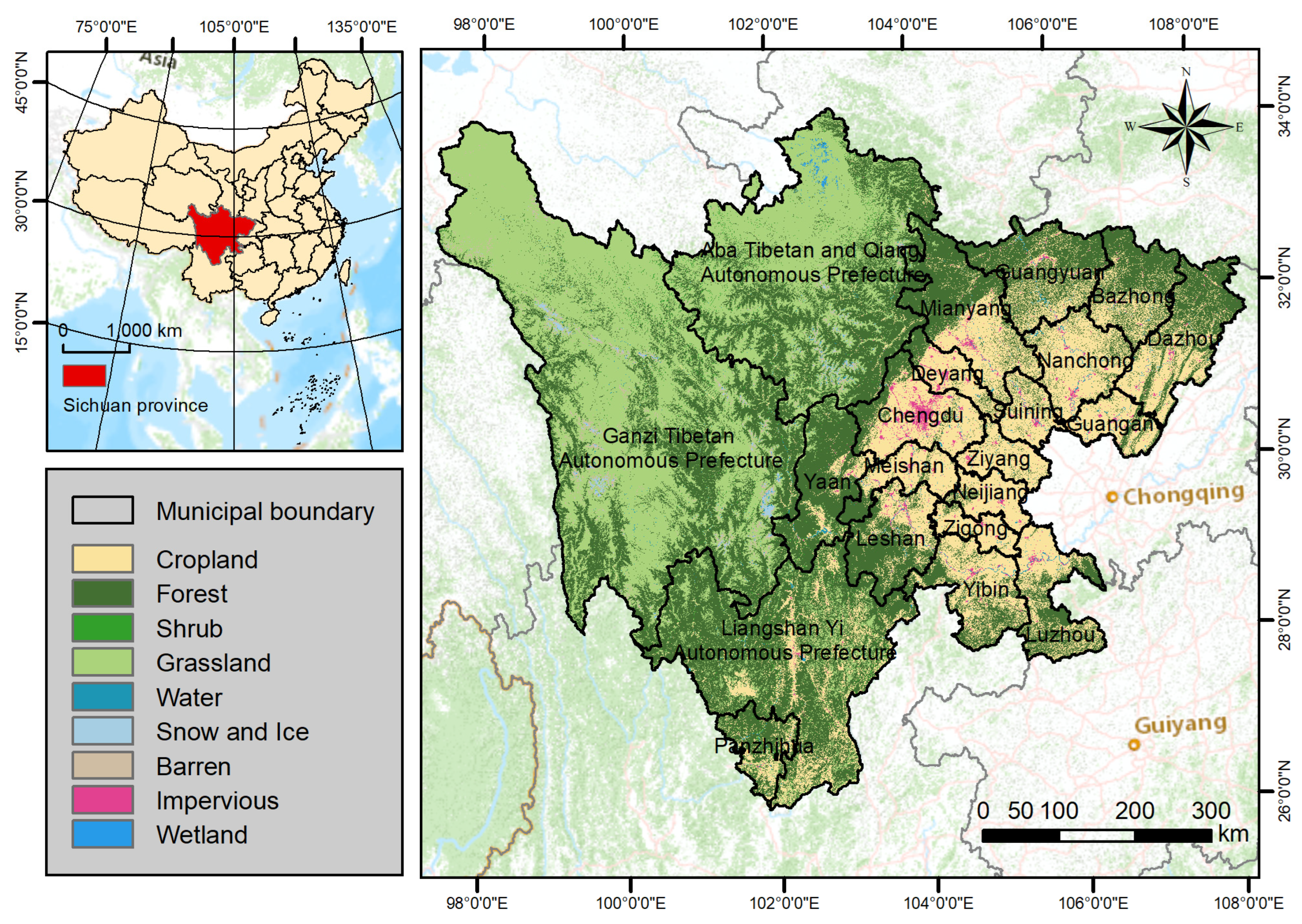
2.1. Study Area

As the economic development center of southwest China, Sichuan Province is an integral part of the national development strategy. It is also one of the 13 central grain-producing provinces in the country and the only central grain-producing province in the west. In 2020, Sichuan’s grain yield ranked 9th in the country. As shown in Figure 1, Sichuan Province is located between 26°03′–34°19′ north latitude and 97°21′–108°12′ east longitude. It is inland in southwest China and the upper reaches of the Yangtze River. Sichuan Province is located on the first and second levels of the three significant terrain ladders in China’s mainland, that is, in the transition zone between the first-level Qinghai-Tibet Plateau and the second-level plain source of the middle and lower reaches of the Yangtze River [30]. There is a significant difference between the east and west; the terrain is high in the west and low in the east. Sichuan’s landforms are complex, with mountains as the main feature, and there are four landform types: mountains, hills, plains, and plateaus. The climate of the Sichuan Province is also very different. In the Sichuan Basin, the eastern part has a humid subtropical climate; the southwest has a mountainous semi-humid climate; and the northwest has an alpine and plateau alpine climate. Sichuan Province’s topographic characteristics and climate conditions primarily distribute its agricultural planting areas in the eastern basin, with rice, corn, and wheat being the most commonly grown crops. In recent years, problems such as non-grain conversion of cropland, cropland abandonment, and farmland fragmentation have gradually intensified, posing a threat to the food security of Sichuan Province. At the same time, Sichuan Province is also actively carrying out LC projects. In the latest round of comprehensive LC planning (2016–2020), Sichuan Province has implemented a total of 1581 land development and consolidation projects, adding 68,200 hectares of cropland; the infrastructure conditions for agricultural production have been improved, referred to as high-standard farmland, with 107,900 hectares. Grain production has increased by 66,190 kg due to the improved cropland quality, and both the area and quality of cropland have significantly improved.

2.2. Sources of Data

The data used in this paper mainly include remote sensing data, project area data, and other dataset products, and the specific data information and sources are shown in

Table 1. Information and sources of data.

Data	Classification	Resolution	Time	Data source
Landsat 8	raster	30 m	2017–2024	https://www.usgs.gov (accessed on 12 December 2023)
Sentinel-2	raster	10 m	2017–2024	https://www.esa.int (accessed on 12 December 2023)
LC project	vector	/	2020	Sichuan Provincial Government (accessed on 5 March 2022)
DEM	raster	30 m	2022	https://panda.copernicus.eu/panda (accessed on 3 January 2024)
SOC	raster	250 m	1950–2017	https://data.isric.org/geonetwork (accessed on 3 January 2024)
Rainfall	raster	1 km	2020	https://www.gis5g.com (accessed on 3 January 2024)

“/” indicates that the data does not have the relevant attribute.

.

2.2.1. LC Project Data

The project area data used in this article come from the Sichuan Province LC project database, which contains approximately 5800 LC projects in Sichuan Province from 1999 to 2020. The data include project number, name, category, administrative region, acceptance date, total project investment, and other information. It should be noted that due to the limitation of the number of effective observations of the selected satellites, the number of effective observations in 2016 was significantly higher than that in 2015, with a median of more than 24 times, which can ensure the fidelity of the time series, so we selected the time period after 2016 as the optional research time period. At the same time, to ensure that the number of years before and after LC is at least three years and consistent, we selected 227 LC projects with the project date “2020” and used 2017 to 2024 as the specific research time period. All LC projects were completed and accepted in 2020.

2.2.2. Sentinel-2 A/B and Landsat 8

To solve the problem that a single MODIS satellite is not suitable in areas with complex topography, such as mountains and hills, we combined Landsat 8 OLI and Sentinel-2A/B MSI, and their data processing level is the top of the atmosphere (TOA). Landsat8 OLI is provided by NASA and the United States Geological Survey (USGS), and Sentinel-2 MSI is provided by the European Space Agency (ESA). Among them, Landsat 8 was launched in 2013, with a spatial resolution of 30 m and a revisit period of 16 days; the Sentinel-2A/B binary stars were launched in 2015 and 2017, respectively, with a maximum spatial resolution of 10 m, the double star revisit period is once every five days.

2.2.3. Geospatial Data

The elevation data used in this study are the 2022 Copernicus DEM data with a spatial resolution of 30 m, released by the European Space Agency (https://panda.copernicus.eu/panda (accessed on 3 January 2024)); the precipitation data come from the development of the Earth Resources Data Cloud Platform China’s 1 km resolution annual average rainfall dataset (https://www.gis5g.com (accessed on 3 January 2024)), which is obtained by interpolation based on data from 2472 meteorological observation points across the country; soil organic carbon content data were produced by Professor Tomislav Hengl (https://data.isric.org/geonetwork (accessed on 3 January 2024)), the data are based on a compilation of global soil profiles and samples from 1950 to 2017 obtained by using R language machine learning, with a spatial resolution of 250 m.

2.3. Research Methods

The overall technical framework for identifying LC capacity changes and analyzing effect attribution is shown in Figure 2. The workflow mainly includes four essential steps. First, we used multi-source remote sensing data Landsat 8 and Sentinel-2 A/B, which were normalized, cloud masked, and S-G filtered to obtain NDVI time series at 10-day intervals, and computed annual CumVI using an integration algorithm to characterize annual cropland yield; secondly, we proposed a characteristic parameter method to identify changes in productivity to identify changes in yield level and yield stability before and after LC, and divided the effectiveness of LC into four types type; then, we used the hotspot analysis method to explore the spatial differentiation of LC effectiveness; finally, based on four natural condition factors, we obtained the average value of each project area through zoning statistics, and used GeoDetector and GWR to analyze the impact of natural conditions on the effectiveness of LC.

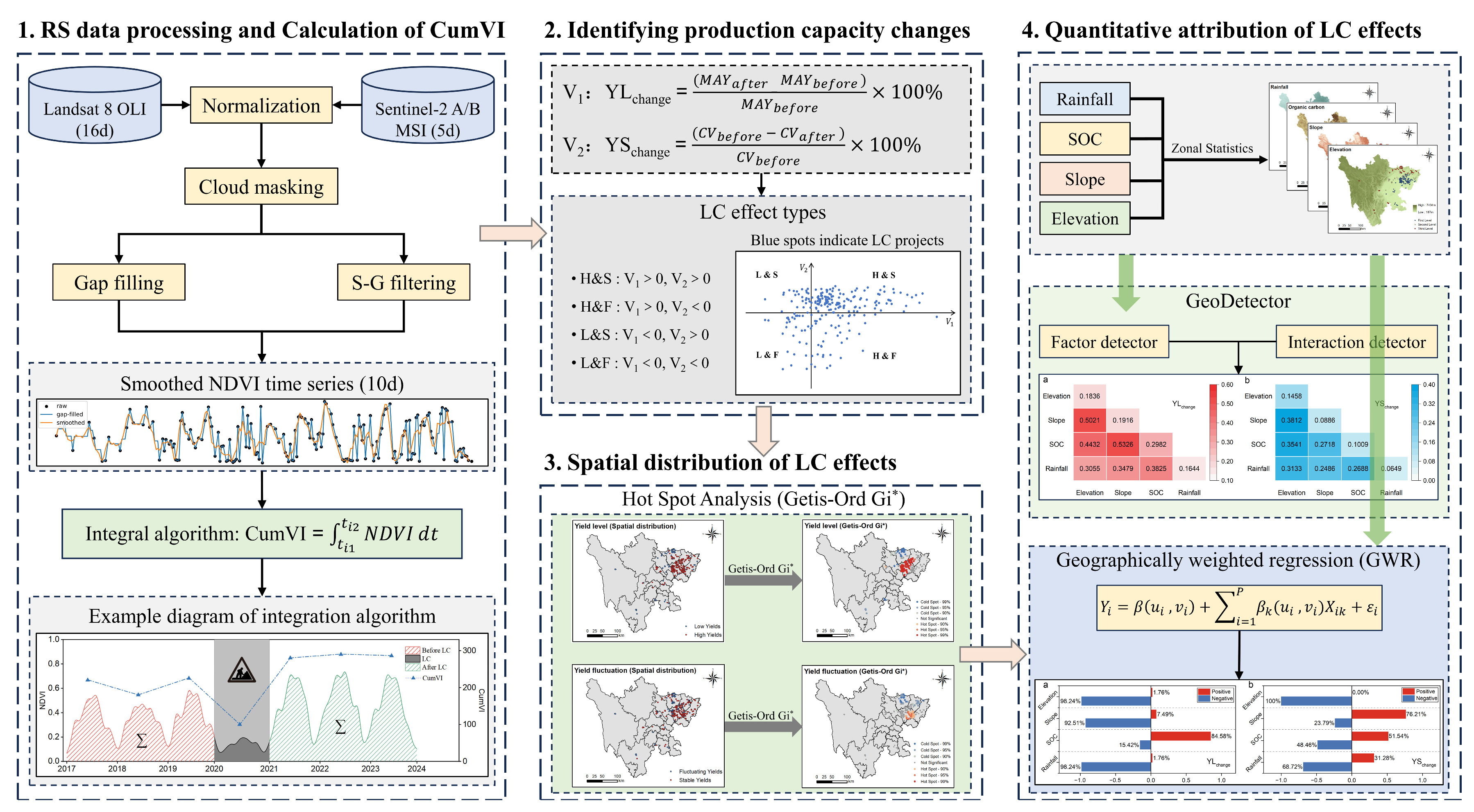
2.3.1. Remote Sensing Data Processing and CumVI Calculation

Due to the differences in spectrum and reflectance between OLI and MSI, they must be coordinated to obtain stackable results. Zhang et al. proposed a method using ordinary least squares (OLS) linear regression to normalize the two sensors, improve the consistency between Sentinel-2A MSI and Landsat-8 OLI data, and obtain a higher degree of fitting [31]. Based on this method, we normalized the NDVI calculated by Landsat-8 to the NDVI of Sentinel-2 A/B to reduce the NDVI difference caused by factors such as satellite spectral response functions. The quality band was combined with satellite data to reduce cloud contamination and oversaturation. Then, we used the maximum value synthesis approach to generate a ten-day time series for the non-uniformly collected NDVI data. We utilized a linear function to fill in the missing values in the middle, followed by the SG filter technique to smooth and erase the NDVI pixels. After considering the influence of residual clouds, haze, and other factors, we obtained the NDVI time series evenly sampled at 10-day intervals.

Johnson et al. used the MODIS NDVI to evaluate corn and soybean yields in the United States. The results showed that corn and soybean yields positively correlate with the NDVI [32]. Therefore, we calculated the integral sum of the smoothed NDVI time series by year to obtain CumVI. The total annual yield can be characterized, and the formula is as follows:

$$\mathrm{C}\mathrm{u}\mathrm{m}\mathrm{V}\mathrm{I}={\int }_{t_{i1}}^{t_{i2}}\mathrm{N}\mathrm{D}\mathrm{V}\mathrm{I} dt$$

(1)

In the formula, the NDVI is the value after SG filtering, and t_i1 and t_i2 are the starting and ending times of the i-th year time series, respectively.

2.3.2. Characteristic Parameter Method to Identify Production Capacity Changes

LC improves farmland farming conditions and the environment for agricultural production through comprehensive consolidation and optimized allocation. Existing studies generally believe LC can effectively improve agricultural production capacity to ensure food security and increase farmers’ income [33,34]. In an ideal world, the impact of LC on productivity can be reflected in two aspects: an increase in yield level due to improved farming conditions and an increase in inter-annual yield stability. Therefore, we used two indicators to evaluate the effect of LC: the first V₁ is the change rate of yield level before and after LC (YL_change), and the second V₂ is the change rate of yield stability before and after LC (YS_change). The calculation formulas are as follows Equations (2) and (3), where the mean annual yields before and after consolidation (MAY_before/after) are the annual CumVI before and after consolidation, and the coefficient of variation before and after consolidation (CV_before/after) are the standard deviation of annual CumVI before and after consolidation.

$${\mathrm{V}}_1: {\mathrm{YL}}_{\mathrm{change}}=\frac{({\mathrm{M}\mathrm{A}\mathrm{Y}}_{\mathrm{a}\mathrm{f}\mathrm{t}\mathrm{e}\mathrm{r}}-{\mathrm{M}\mathrm{A}\mathrm{Y}}_{\mathrm{b}\mathrm{e}\mathrm{f}\mathrm{o}\mathrm{r}\mathrm{e}})}{{\mathrm{M}\mathrm{A}\mathrm{Y}}_{\mathrm{b}\mathrm{e}\mathrm{f}\mathrm{o}\mathrm{r}\mathrm{e}}}\times 100\mathrm{\%}$$

(2)

$${\mathrm{V}}_2: {\mathrm{YS}}_{\mathrm{change}}=\frac{({\mathrm{C}\mathrm{V}}_{\mathrm{b}\mathrm{e}\mathrm{f}\mathrm{o}\mathrm{r}\mathrm{e}}-{\mathrm{C}\mathrm{V}}_{\mathrm{a}\mathrm{f}\mathrm{t}\mathrm{e}\mathrm{r}})}{{\mathrm{C}\mathrm{V}}_{\mathrm{b}\mathrm{e}\mathrm{f}\mathrm{o}\mathrm{r}\mathrm{e}}}\times 100\mathrm{\%}$$

(3)

Therefore, when V₁ > 0, it means that LC is efficacious in improving yield level, and the average annual yield after LC increases; when V₂ > 0, it means that LC is efficacious in improving yield stability, the inter-annual yield volatility after LC is reduced and the stability is improved. As shown in

Table 2. Classification of LC effects and interpretation of indicators.

	H and S	H and F	L and S	L and F
Full name	High and stable yield	High and fluctuating yield	Low and stable yield	Low and fluctuating yield
Index	V1 > 0, V2 > 0	V1 > 0, V2 < 0	V1 < 0, V2 > 0	V1 < 0, V2 < 0

, we can divide the LC effect into four types: high and stable yield (H and S), high and Fluctuating yield (H and F), low and stable yield (L and S), and low and fluctuating yield (L and F).

2.3.3. Research on the Spatial Distribution of LC Effectiveness

Based on ArcGIS, this study conducted a hotspot analysis (Getis-Ord Gi*) on the LC effectiveness (YL_change and YS_change) to explore its spatial cluster characteristics. The Getis-Ord Gi* index is mainly used to detect space aggregation. The core idea is to calculate the local sum of an element and its neighboring elements within a given distance compared to the sum of all elements. It is used to analyze the degree of clustering of attribute values at the local spatial level [35]. The formula is:

$${\mathrm{G}\mathrm{i}}^{\ast }=\frac{\sum _{\mathrm{j}=1}^{\mathrm{n}}{\mathrm{W}}_{\mathrm{i}\mathrm{j}}\left(\mathrm{d}\right){\mathrm{X}}_{\mathrm{j}}}{{\sum }_{\mathrm{j}=1}^{\mathrm{n}}{\mathrm{X}}_{\mathrm{j}}}$$

(4)

Among them, X_j is the attribute value of element j, W_ij is the spatial weight between elements i and j, and n is the total number of elements. The statistical test of the Getis-Ord Gi* statistic can be expressed according to the corresponding standardized form (Z value), as expressed in Equation (5):

$${\mathrm{Z}(\mathrm{G}\mathrm{i}}^{\ast })=\frac{{\sum }_{\mathrm{j}=1}^{\mathrm{n}}{\mathrm{W}}_{\mathrm{i}\mathrm{j}}{\mathrm{X}}_{\mathrm{j}}-\overline{\mathrm{X}}\sum _{\mathrm{j}=1}^{\mathrm{n}}{\mathrm{W}}_{\mathrm{i}\mathrm{j}}}{\sqrt{\frac{{\sum }_{\mathrm{j}=1}^{\mathrm{n}}{\mathrm{X}}_{\mathrm{j}}^2}{\mathrm{n}}-{\left(\overline{\mathrm{X}}\right)}^2}\sqrt{\frac{\left[\mathrm{n}\sum _{\mathrm{j}=1}^{\mathrm{n}}{\mathrm{W}}_{\mathrm{i}\mathrm{j}}^2-{\left({\sum }_{\mathrm{j}=1}^{\mathrm{n}}{\mathrm{W}}_{\mathrm{i}\mathrm{j}}\right)}^2\right]}{\mathrm{n}-1}}}$$

(5)

When the value of Z is greater than 0, it indicates high-value spatial agglomeration, and the larger the value of Z is, the more significant the agglomeration is; when the value of Z is less than 0, it indicates low-value spatial agglomeration, and the smaller the value of Z is, the more significant the agglomeration is; when the value of Z is equal to 0, it indicates that the agglomeration is not substantial.

2.3.4. Quantitative Attribution of Natural Factors for LC Effectiveness

(1) GeoDetector

GeoDetector is a set of statistical methods that detect spatial differentiation and reveal the driving forces behind it [36]. The rationale is that when the spatial distributions of the explanatory and explanatory variables are more similar, the effect of the explanatory variable on the explanatory variable is more significant [37]. The formula is shown in (6):

$$\mathrm{q}=1-\frac{1}{\mathrm{N}{\mathsf{\sigma }}^2}{\sum }_{\mathrm{h}=1}^{\mathrm{L}}{\mathrm{N}}_{\mathrm{h}}{\mathsf{\sigma }}_{\mathrm{h}}^2$$

(6)

In the formula, the value of “q” represents the index of the spatial differentiation of the influence of the four types of natural condition factors on the effect of LC, and the more significant the value, the greater the impact; “h = 1, 2 … L” is the classification of the four types of natural condition factors; “N_h” and “N” are the number of units in the h-level region and the entire region, respectively; “${\mathsf{\sigma }}^2$” and “${\mathsf{\sigma }}_{\mathrm{h}}^2$” are the variance of the LC effectiveness for the whole area and the area at level “h”, respectively.

In addition, we used GeoDetector to detect the interaction of four natural condition factors to determine whether the explanatory power of the dependent variable is enhanced or weakened when two influences act together, or whether the effects of these factors on the dependent variable are independent of each other [36]. The following five situations will occur after the interaction of two factors:

Nonlinear weakening: q(X₁∩X₂) < min(q(X₁), q(X₂));

Single factor nonlinear weakening: min (q(X₁), q(X₂)) <q(X₁∩X₂) < max(q(X₁), q(X₂));

Two-factor enhancement: max(q(X₁), q(X₂)) < q(X₁∩X₂) < q(X₁) + q(X₂);

Independent: q(X₁∩X₂) = q(X₁) + q(X₂);

Nonlinear enhancement: q(X₁∩X₂) > q(X₁) + q(X₂);

Among them, q(X₁∩X₂) represents the maximum effect of X₁ and X₂; q(X₁) + q(X₂) represents the sum of the effects of X₁ and X₂.

(2) Geographically weighted regression (GWR)

Traditional linear regression models (OLS models) only estimate all samples and parameters globally and do not incorporate the consideration of elements such as spatial patterns [38]. GWR is solved through a local weighted regression analysis model about the position and uses parameter estimation results that change with different spatial positions to quantitatively reflect the heterogeneity or non-stationary characteristics in the spatial data relationship [39]. Therefore, we used the GWR model to perform the analysis. We compared the parameters of OLS and GWR in the follow-up results to verify the suitability of the GWR model. The formula is as shown in Equation (7) Show:

$${\mathrm{Y}}_{\mathrm{i}}={\mathsf{\beta }}_0\left({\mathrm{u}}_{\mathrm{i}},{\mathrm{v}}_{\mathrm{i}}\right)+{\sum }_{\mathrm{i}=1}^{\mathrm{P}}{\mathsf{\beta }}_{\mathrm{k}}\left({\mathrm{u}}_{\mathrm{i}},{\mathrm{v}}_{\mathrm{i}}\right){\mathrm{X}}_{\mathrm{i}\mathrm{k}}+{\mathsf{\epsilon }}_{\mathrm{i}}$$

(7)

${\mathrm{Y}}_{\mathrm{i}}$ represents the value of the dependent variable at position i; ${\mathrm{X}}_{\mathrm{i}\mathrm{k}}$ is the value of the independent variable k at position; ${\mathsf{\beta }}_{\mathrm{k}}\left({\mathrm{u}}_{\mathrm{i}},{\mathrm{v}}_{\mathrm{i}}\right)$ and ${\mathsf{\beta }}_0\left({\mathrm{u}}_{\mathrm{i}},{\mathrm{v}}_{\mathrm{i}}\right)$ are, respectively, the coefficients and intercepts of the regression model established by GWR at position i, P represents the number of predictor variables; ${\mathsf{\epsilon }}_{\mathrm{i}}$ is the regression residual of point i; $\left({\mathrm{u}}_{\mathrm{i}},{\mathrm{v}}_{\mathrm{i}}\right)$ represents the spatial position of point i.

3. Results

3.1. Typical Processes and Characteristics of LC Effectiveness

As shown in Figure 3a, this article listed NDVI time series diagrams of four typical project areas to represent the productivity changes in the above four LC effects. Among them, “Gap-filled” represents the NDVI curve obtained by linear filling of the original measurement data, and “Smoothed” represents the NDVI curve after S-G smoothing. The table on the correct records the names of four typical project areas and the values of CumVI, YL_change, and YS_change indicators each year before and after LC. The NDVI time series curve is similar to the trend of a sinusoidal function. In each annual period, the NDVI first has an upward trend, which is caused by the growth and development of crops; when reaching a specific peak value, the NDVI begins to decrease, which is caused by harvesting. In addition, different types of LC effects also have different NDVI time series curves. For example, the “LC project in Panlong Township, Nanbu County”: before LC (2017–2020), the total annual yield of farmland remained at a low level (CumVI < 0.3), with inter-annual fluctuations also relatively large; during the LC stage (2020–2021), since project implementation makes a certain degree of intervention on the land, the NDVI will further decline, and it will take some time to return to a higher and stable level; when the LC project is completed (after 2021), agricultural production capacity will return to a high and stable level (CumVI > 0.3).

As shown in Figure 3b, among the 227 LC projects in Sichuan Province in 2020 selected in this study, the average value of V₁ is 7.74%, the maximum value is 47.91%, and the minimum value is −17.60%, indicating that some project areas have decreased yield levels after LC; the average value of V₂ is 12.40%, the maximum value is 95.44%, and the minimum value is −201.35%, indicating that some project areas have decreased yield stability after LC.

As shown in Figure 3c, a total of 126 project areas have achieved increased yield level and improved stability, accounting for 55.51% of the total number of project areas; 45 project areas have increased yield level but decreased stability, and 26 project areas have decreased yield level but increased stability, which together account for 31.27% of the total number of project areas; a total of 30 project areas, or 13.22% of the total number of project areas, had declining yield level and decreased stability.

In summary, the 2020 LC project in Sichuan Province effectively enhanced yield level and stability. The average improvement rates of the two are 7.74% and 12.40%, respectively. Over half of the project area has achieved the dual effect of increasing and stabilizing production. However, after implementing LC projects, production capacity regression in some project areas remains a problem.

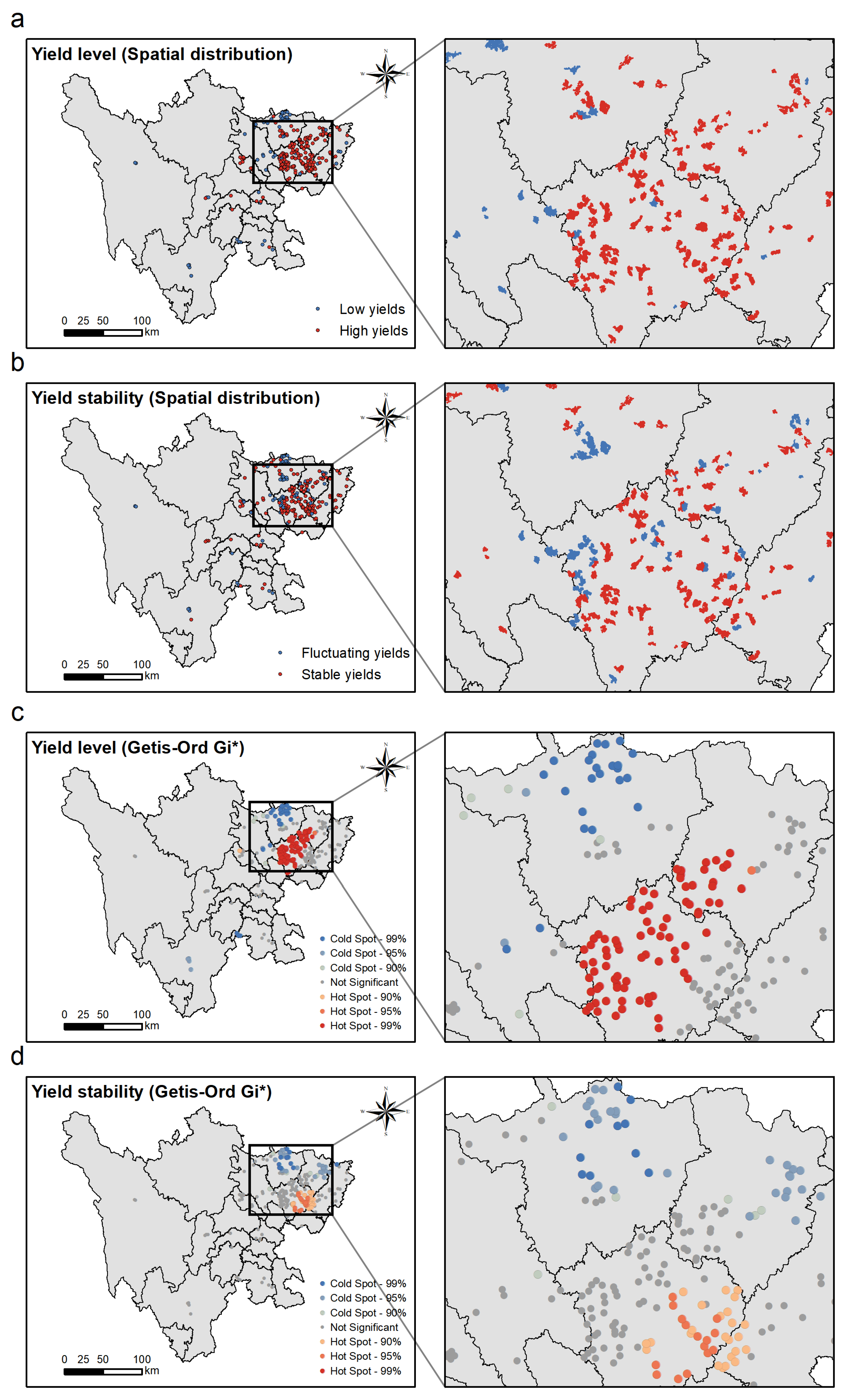
3.2. Spatial Distribution of LC Effectiveness

We explored the characteristics of the spatial distribution of YL_change and YS_change and analyzed their spatial correlation using Getis-Ord Gi*. Figure 3 shows that the 2020 LC project areas in Sichuan Province are mainly distributed in the northeastern region, with most of them in Nanchong City, Guangyuan City, Bazhong City, and Dazhou City. Scattered project areas in central and southern Sichuan Province are distributed in Ya’an City, Meishan City, Ziyang City, Yibin City, and Liangshan Yi Autonomous Prefecture.

From Figure 4a,c, it can be seen that the project areas realizing yield level improvement in 2020 are mainly distributed in Nanchong City and its surrounding areas and show a centralized and contiguous distribution; the project areas with reduced yield level, on the other hand, are mainly located in the northern part of Guangyuan City, the northwestern and southeastern parts of Mianyang City, the Liangshan Yi Autonomous Prefecture, and the Ganzi Tibetan Autonomous Prefecture, showing a more discrete distribution pattern. The Getis-Ord Gi* analysis shows that the high values of yield level increase are distributed in Nanchong City with a 99% confidence level, and the low values are mainly distributed in the northern part of Guangyuan City with a 99% confidence level, which indicates that the spatial distributions of both high and low values of yield level are correlated, and the clustering of high values is more significant.

It can be seen from Figure 4b,d that the project areas with increased yield stability are mainly located in Nanchong City, with discrete distribution in Mianyang City, Bazhong City, and Dazhou City, while the project areas with decreased yield stability are mainly located in the northern part of Guangyuan City, with distribution in the western part of Nanchong City and Bazhong City. It is worth noting that the results of the Getis-Ord Gi* analysis of yield stability show that high-value agglomerations are distributed only in the southwestern part of Nanchong City, and the confidence level is lower than 99%; low-value agglomerations are mainly distributed in the northern part of Guangyuan City and the eastern part of Bazhong City, etc., with a confidence level of 95%, which indicates that the spatial distributions of high and low values of yield stability are equally correlated, but the significance level of the distribution of the correlation of the latter is lower compared the former.

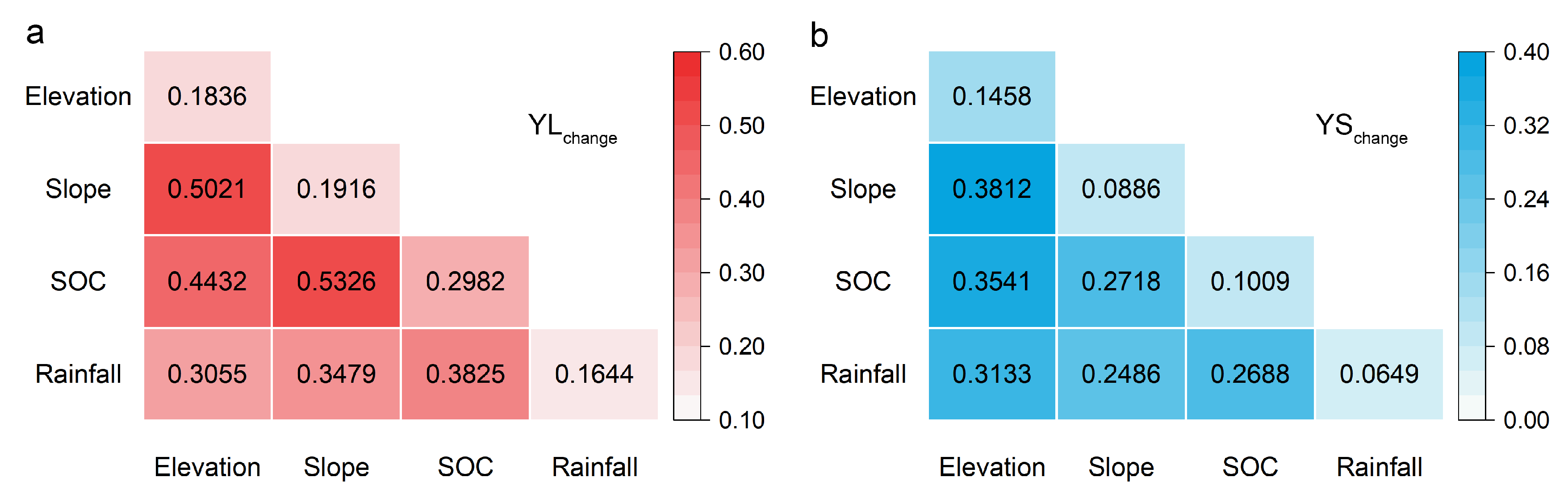
3.3. Natural Attribution of LC Effectiveness Based on GeoDetector

To study the factors influencing the effectiveness of LC, this study selected four types of natural condition factors: elevation, slope, soil organic carbon (SOC), and rainfall. Elevation and slope can mirror the intricacy of the topographic conditions in the project area; soil organic carbon (SOC) is a crucial component of soil, considered the core of soil quality and function [40], and a decisive factor influencing soil fertility [41]. Water also plays a significant role in crop growth [42], while rainfall reflects the water environment in the project area. We used the “nature breaks” method to divide the four types of natural conditions into five levels. Then, we utilized GeoDetector to analyze the degree of influence and interaction of factors on LC effectiveness.

As shown in

Table 3. LC effect divergence and factor detection.

	YLchange			YSchange
Factors	q	p		q	p
Elevation	0.1836	0.000	3	0.1458	0.011	1
Slope	0.1916	0.000	2	0.0886	0.000	3
SOC	0.2982	0.000	1	0.1009	0.007	2
Rainfall	0.1644	0.000	4	0.0649	0.048	4

, in the results of GeoDetector’s factor detection: “factors” enumerate four different natural condition factors; the q-value measures the extent to which factor X explains the spatial differentiation of attribute Y, that is the degree of influence on the LC effect; the p-value represents the significance test result of the q value, and all factors passed the significance test. The result of the q value of YL_change is SOC (0.2982) > slope (0.1916) > elevation (0.1836) > rainfall (0.1644). It can be seen that SOC is the most critical influence on YL_change, with slope, elevation and rainfall remaining in that order. The q-value result of YS_change is elevation (0.1458) > SOC (0.1009) > slope (0.0885) > rainfall (0.0649). It can be seen that elevation is the most critical influence on YS_change, with SOC, slope, and rainfall remaining in that order.

As shown in Figure 5a, in the results of GeoDetector interaction detection, six interaction categories exist among the four types of natural condition factors. All interactions of both two factors on the spatial differentiation of land preparation yield levels are greater than the effect of either variable alone; in particular, interactions of slope∩SOC and elevation∩slope are greater than the independent sum of the two, which are nonlinearly augmented, while the interactions of the remaining factors are two-way augmented; moreover, the interaction effects of slope∩SOC and elevation∩slope are significant, and the q value is greater than 0.5. As shown in Figure 5b, among the interactions on YS_change, all interactions between two factors on the spatial differentiation of LC yield stability are greater than the effect of the two independently added together; all of them are nonlinear enhancements; interactions of elevation∩slope and elevation∩SOC are more significant.

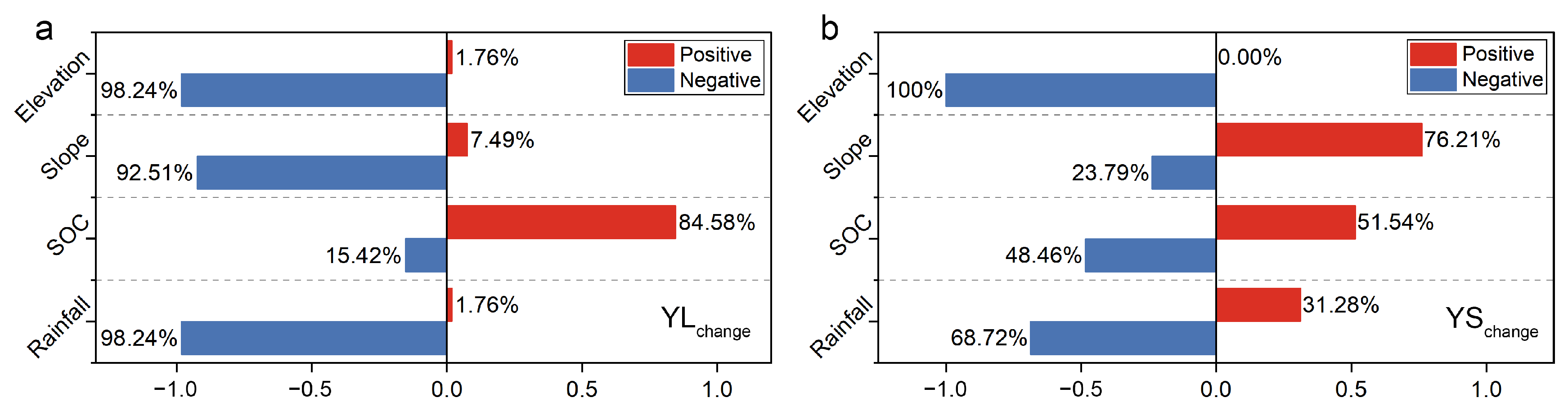
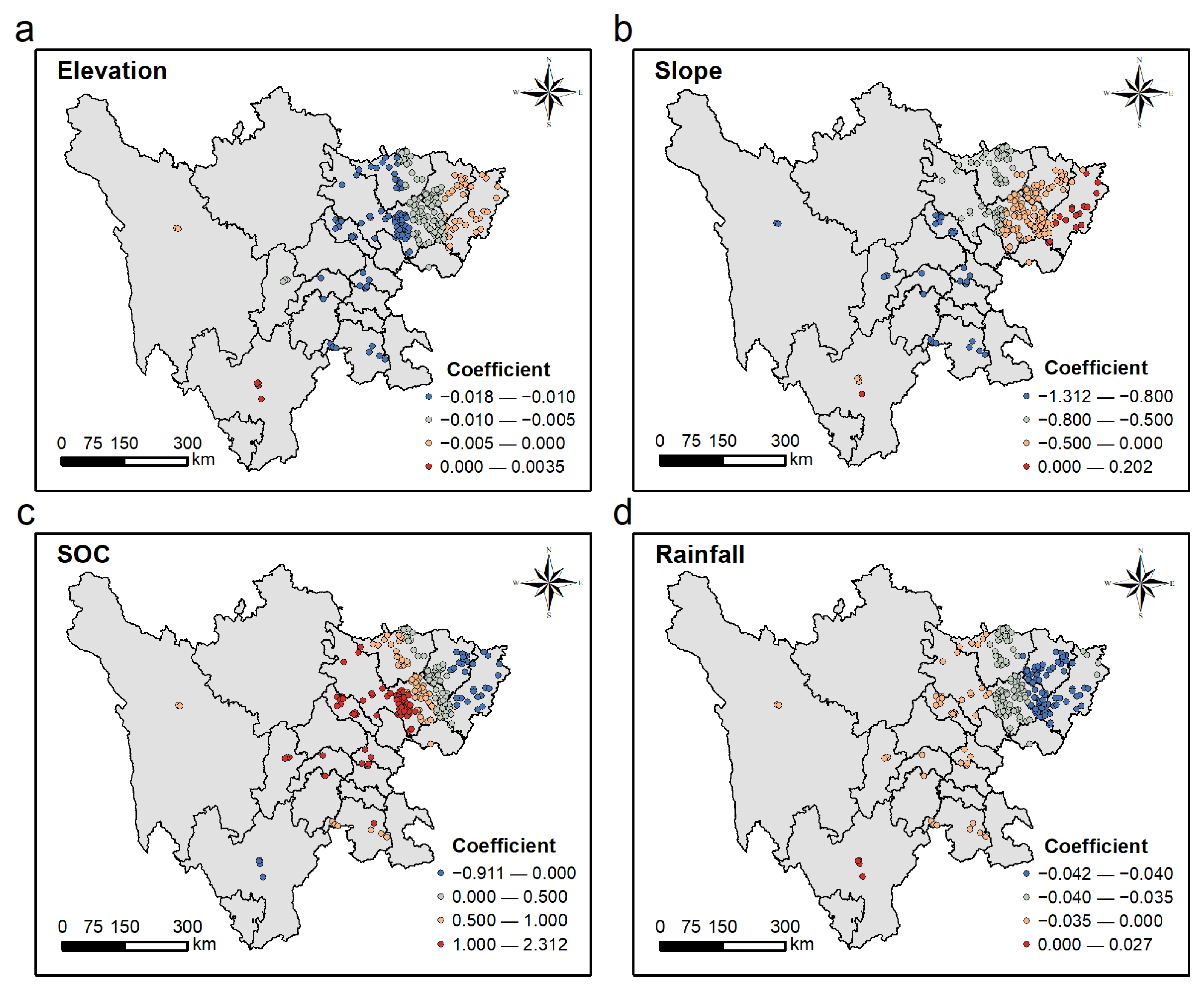
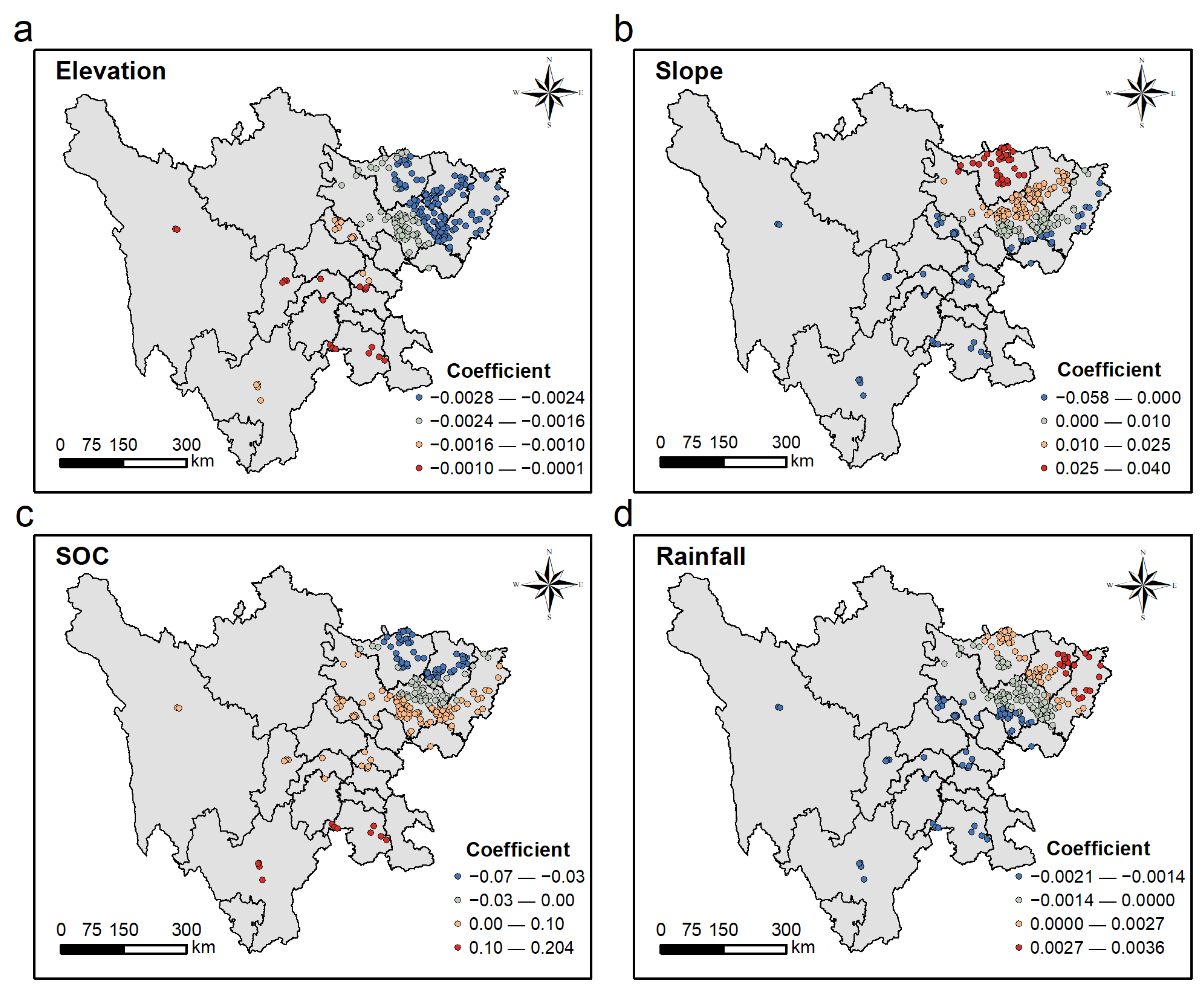
3.4. Natural Attribution of LC Effectiveness Based on GWR

GeoDetector can only explore the degree of influence and interaction of different factors on the LC effectiveness and cannot show the trend of influence of independent variables on dependent variables. This study used GWR to perform regression analysis on LC yield level and yield stability. It should be noted in advance that the total investment in LC projects in Sichuan Province is standardized and positively correlated with the size of the project area, so the investment amount per unit in different project areas is roughly the same, thus eliminating the impact of project investment on the effectiveness of LC projects.

Table 4. Parameter comparison of OLS and GWR.

	YLchange			YSchange
Model	R2	Adj.R2	AICc	R2	Adj.R2	AICc
OLS	0.514	0.505	167.42	0.205	0.191	257.76
GWR	0.886	0.843	85.76	0.661	0.554	101.69

compares the model parameters of OLS and GWR. It can be seen that compared with OLS, the Adj.R² of the GWR model is more extensive, and the AICc of the GWR model is also smaller, indicating that the GWR model has a better fitting degree.

As shown in Figure 6a and Figure 7, the influence trends of the four natural conditions factors on YL_change differ. The coefficient estimates of elevation, slope, and rainfall are mainly negative, indicating that they negatively affect the improvement of YL_change.The negative impact of elevation, slope, and rainfall account for 98.24%, 92.51%, and 98.24%, respectively. In addition, the intensity of impacts varies from region to region; for example, the absolute value of the rainfall coefficient gradually decreases from east to west, and the negative effect gradually weakens accordingly. For SOC, its coefficient estimate is mainly positive, indicating that SOC positively impacts the improvement of YL_change. The proportion of the positive effect is 84.58% and gradually weakens from south to north. However, a noteworthy negative effect of 15.42% remains, mainly distributed in areas such as Guangyuan City, Bazhong City, and the northern part of Nanchong City.

As shown in Figure 6b and Figure 8, the influence trends of the four natural condition factors on YL_change are also different and more complex.The coefficient estimates for elevation are all negative, indicating that it has a single inhibitory effect on YS_change, with the negative effect diminishing from northeast to southwest. Slope has 76.21% positive effect and 23.79% negative effect; SOC has 51.54% positive effect and 48.46% negative effect; rainfall has 31.28% positive effect and 68.72% negative effect. It suggests that the effects of the three on YS_change are more complex, with more pronouncedly opposite trends across geographic locations.

4. Discussions

4.1. Advantages and Advancements

This study used remote sensing data to analyze the productivity changes and influencing factors of the LC project area in Sichuan Province in 2020. Compared with traditional research methods, remote sensing technology has the characteristics of comprehensive coverage, long time, and high accuracy and can more accurately determine the productivity characteristics of cropland. Machine learning and deep learning algorithms have developed rapidly in recent years and have been widely used in recognizing cropland information and predicting crop yields. However, this method mainly relies on establishing the correlation between yield and characteristic variables, which greatly depends on field sampling or actual measured yield data. This study establishes a relative yield relationship, which does not depend on actual measured yield data. Therefore, it greatly reduces the cost of data acquisition and is an efficient acquisition method. However, it should also be seen that our study does not utilize the actual measured yield data, so the measured yield is not the absolute capacity of arable land. However, it has a good advantage in the field of analyzing the effect of land consolidation on the capacity of cropland. We used a combination of Sentinel and Landsat satellites to generate NDVI time series data, then used the SG filtering algorithm to fill it out smoothly. In this paper, two satellites, Sentinel and Landsat, were combined to generate NDVI time series data, filled and smoothed using the S-G filtering algorithm, followed by linear interpolation to generate 10 m spatial resolution images. This approach dramatically improves temporal and spatial accuracy and solves the problem of single MODIS satellite data not being applicable in areas with complex topography, such as mountainous hills. This paper also breaks through the limitations of traditional research at a single time node by constructing an NDVI time series before and after LC. In addition, our project area data come from Sichuan Province, so it is more precise and has a wider study scale compared to a single project area, which can explore the regularity of the effect of land consolidation differences from a more macroscopic point of view. Most of the studies on similar topics only drew on existing experience to speculate on the factors affecting land consolidation effectiveness [26], without using real data to analyze the influencing factors of land consolidation effectiveness from a quantitative perspective. In contrast, this study utilized GeoDetector and GWR models to quantitatively analyze the impacts of the four natural factors, respectively, to reveal the regularity of the influence of natural conditions on the effectiveness of LC. Therefore, this study is of a certain degree of cutting-edge and reference significance. Our results show that land consolidation can effectively improve the productivity of arable land in general, but there are still some project areas where the productivity of arable land decreases after land consolidation. Du et al. measured China’s land consolidation project areas in 2006 and 2007 using NDVI data [27]. Their results showed that in 2006 and 2007, 78.67% and 78.32% of the project areas experienced either improved or stabilized productivity following the LC. However, there were also project areas where productivity declined or fluctuated. This indicates that land consolidation can enhance the productivity of arable land significantly. Their study shares similarities with our findings, providing additional support for the validity of this study.

4.2. The Impact and Inspiration of LC on Farmland Productivity

The average improvement rate of yield level of LC projects in Sichuan Province in 2020 is 7.74%, and the average improvement rate of yield stability is 12.40%; more than half of the project areas have achieved both an increase in yield level and yield stability. LC mainly improves farmland capacity through two aspects: strengthening agricultural infrastructure to support an increase in yield per unit area, or conducting land formation and field consolidation to increase planting area [27]. However, there are still problems with some projects experiencing a decrease in average annual yield or an increase in inter-annual yield fluctuations after implementing LC projects. This may be due to certain defects in the project’s construction, such as irrational construction that may damage the soil layer, affecting the cropland’s quality. Improper post-project management may also make it difficult to put the consolidated land into use, which may be due to the Chinese particular land ownership structure. In addition to the above, there may be certain external factors: the abandonment of cropland due to economic backwardness, poor geography, etc., may also cause a decline in cropland productivity [43]. Moreover, weather and climate are key driving factors that affect the productivity of agricultural systems [44]. Therefore, there may be a phenomenon where climatic conditions become severe after LC, resulting in a serious decline in farmland productivity, and the improvement of farmland capacity from LC cannot be effectively demonstrated.

Revealing the natural attribution of productivity changes can provide enlightenment for LC work. Regarding explaining the spatial differentiation of the LC yield level, the Adj.R² of the GWR model is 0.843, indicating that the four natural factors have good explanatory power on the LC yield level. SOC is the most important influencing factor, mainly showing a positive effect. This indicates that the larger the SOC, the higher the fertility potential of the soil [45], the greater the potential that can be stimulated after the implementation of LC, and therefore, the more significant the increase in yield level. Further, the interaction between elevation and slope also has a non-negligible influence. Both of them together show a negative effect. This indicates that the complexity of topographic and geomorphological conditions makes implementing and managing LC projects more difficult. For example, in the northern part of Guangyuan City and the northwestern part of Mianyang City, which are located on the northwestern edge of the Sichuan Basin, the elevations and slopes are larger, and the yield level of arable land is less elevated. On the contrary, in the central part of Nanchong City, where the elevation and slope are smaller, the yield level of arable land is higher. Rainfall mainly has a negative effect on the yield level of LC, which shows that in areas with low rainfall, LC can vastly improve the problem of water source drought in cropland and improve the yield level of cropland through measures such as building drainage ditches and improving irrigation facilities. The annual precipitation in the Sichuan Basin decreases from the periphery to the center; for example, Nanchong City and the southwestern part of Bazhong City are located in the central hilly area of the Sichuan Basin, and the annual rainfall is less than 900 mm, and the rate of improvement of the level of land consolidation yield is higher; however, the western part of Mianyang City and the eastern part of Dazhou City are located in the western and eastern rims of the Sichuan Basin, respectively, and the rainfall is generally more than 1200 mm, and the rate of improvement of the level of land consolidation yield is generally lower. In terms of explaining the spatial differentiation of LC yield stability, the R² of the GWR model is 0.554, indicating that the four natural factors have relatively poor explanatory power on LC yield stability. In addition, the GeoDetector interaction analysis results also show that the nonlinear enhanced interaction between two factors is much greater than the effect of a single factor. This also suggests that the effects of different factors on the stability of land consolidation yields are not independent of each other, but that there are relatively complex interactions. Elevation is the most critical factor affecting changes in the yield stability of LC, showing a single negative effect, and is the primary consideration for evaluating changes in yield stability. The influence trends of slope, SOC, and rainfall differ in different geographical locations, exhibiting apparent non-stationary effects. The impact of these three factors is relatively weak, but their interaction with other factors is significantly amplified. It also reminds us that we should consider the specific conditions of different regions and evaluate a comprehensive analysis based on various factors.

4.3. Limitations and Future Work

This study analyzed the changes in farmland capacity by comparing the annual CumVI before and after LC. Due to the limited number of effective observations by Sentinel and Landsat satellites, we only calculated the data separately for the three years before and after LC, so there may be some random errors. In addition, due to the relatively short time period across which this study was conducted, we did not take into account the interference with cropland yields caused by human factors such as cropland abandonment, transformation of agricultural land, and cropping structure adjustment, nor did we eliminate the error due to the impact of inter-annual differences in climatic conditions on crop yields. Subsequent research can improve related problems by setting up control areas and controlling variables around the study area. This article only considered natural condition factors, while social, economic, and other factors can also affect the effectiveness of LC; moreover, the specificity of the distribution of the data sample and the limitation of the number of samples can also make the regression results have some errors. Subsequent research can be carried out on a larger scale from more dimensions, such as the natural environment, social economy, and project attributes, to obtain more general and precise regularities and conclusions.

5. Conclusions

In this study, we proposed an NDVI-based method for monitoring LC effectiveness’s spatial and temporal processes and characteristics in Sichuan Province. Based on the data of 227 LC project areas, we integrated Sentinel and Landsat satellites to extract NDVI data. We utilized an integration algorithm to calculate the annual yield of the project areas. We used “YL_change” and “YS_change” indexes to evaluate the effectiveness of LC. Finally, we analyzed the impacts of elevation, slope, SOC, and rainfall on the LC effectiveness using the GeoDetector and GWR model. The results show that the average improvement rate of production level in all project areas in 2020 is 7.74%, and the average improvement rate of production stability is 12.40%. Among them, 55.51% of the project areas have achieved an increase in yield and stability, 19.82% of the project areas achieved an increase in yield but a decrease in stability, 11.45% of the project areas achieved a reduction in yield but an increase in stability, 13.22% of the project areas achieved a reduction in yield and stability. Overall, LC is effective in increasing cropland’s capacity. In space, the yield level and yield stability of LC have clusters of high and low values, and the spatial clustering significance of changes in yield level is more significant than changes in yield stability. In the quantitative attribution of natural factors for the effectiveness of LC, SOC and elevation are the most critical factors affecting the yield level and yield stability of LC, respectively. Different natural factors have different effects on productivity improvement in different regions. Therefore, before the implementation of land consolidation projects, the work can be targeted in the light of local natural conditions. The method proposed in this study for evaluating the effectiveness of land consolidation combines remote sensing and spatial analysis techniques to systematically reveal the regularity of the impact of land consolidation on the productivity of arable land. Our method is significant for designing, implementing, and evaluating land consolidation projects, so it can be popularized and applied to research in related fields. However, the model establishes a relative yield relationship, which does not depend on the actual measured yield data, and the measured results are not the absolute capacity. Although it has a better application in this scenario, it ultimately does not reflect the actual yield change in arable land, so this direction should be improved in the future.

References

1. Van Dijk, M.; Morley, T.; Rau, M.L.; Saghai, Y. A meta-analysis of projected global food demand and population at risk of hunger for the period 2010–2050. Nat. Food 2021, 2, 494–501. [Google Scholar] [CrossRef] [PubMed]
2. Song, X.; Ouyang, Z. Key Influencing Factors of Food Security Guarantee in China during 1999–2007. Acta Geogr. Sin. 2012, 67, 793–803. [Google Scholar] [CrossRef]
3. Fu, Z.; Cai, Y.; Yang, Y.; Dai, E. Research on the relationship of cultivated land change and food security in China. J. Nat. Resour. 2001, 16, 313–319. [Google Scholar] [CrossRef]
4. Potapov, P.; Turubanova, S.; Hansen, M.C.; Tyukavina, A.; Zalles, V.; Khan, A.; Song, X.P.; Pickens, A.; Shen, Q.; Cortez, J. Global maps of cropland extent and change show accelerated cropland expansion in the twenty-first century. Nat. Food 2022, 3, 19–28. [Google Scholar] [CrossRef] [PubMed]
5. Xu, X.; Chen, Q.; Zhu, Z. Evolutionary Overview of Land Consolidation Based on Bibliometric Analysis in Web of Science from 2000 to 2020. Int. J. Environ. Res. Public Health 2022, 19, 3218. [Google Scholar] [CrossRef] [PubMed]
6. Zhu, D.; Lu, Y.; Liu, L. Land Development & Consolidation and Quality Management of Cultivated Land. Trans. Chin. Soc. Agric. Eng. 2002, 18, 167–171. [Google Scholar]
7. Zhang, H. Provincial scale spatial variation of cultivated land production capacity and its impact factors. Trans. Chin. Soc. Agric. Eng. 2010, 26, 308–314. [Google Scholar]
8. Long, H.; Zhang, Y.; Tu, S. Rural vitalization in China: A perspective of land consolidation. J. Geogr. Sci. 2019, 29, 517–530. [Google Scholar] [CrossRef]
9. Jiang, Y. Land consolidation and rural vitalization: A perspective of land use multifunctionality. Prog. Geogr. 2021, 40, 487–497. [Google Scholar] [CrossRef]
10. Li, S.; Song, W. Research Progress in Land Consolidation and Rural Revitalization: Current Status, Characteristics, Regional Differences, and Evolution Laws. Land 2023, 12, 210. [Google Scholar] [CrossRef]
11. Wan, T.; Liu, J.; Tan, Z.; Huang, D. Practice of land consolidation in Germany and its implication to the integrated planning and utilization of collective-owned constructible lands in rural China. City Plan. Rev. 2018, 42, 54–61. [Google Scholar]
12. Du, J.; Sun, P. Review on Land Consolidation Research. J. Shanxi Agric. Sci. 2010, 38, 83–87. [Google Scholar]
13. Lu, D.; Wang, Z.; Su, K.; Zhou, Y.; Li, X.; Lin, A. Understanding the impact of cultivated land-use changes on China’s grain production potential and policy implications: A perspective of non-agriculturalization, non-grainization, and marginalization. J. Clean. Prod. 2024, 436, 140647. [Google Scholar] [CrossRef]
14. Zhao, Q.; Zhou, S.; Wu, S.; Ren, K. Cultivated land resources and strategies for its sustainable utilization and protection in China. Acta Pedol. Sin. 2006, 43, 662–672. [Google Scholar]
15. Lv, X.; Xiao, W.; Li, S.; Wang, Q.; Zhang, C.; Zhang, M. Land reclamation zoning of Chaohu Lake Basin based on GIS and grey constellation clustering. Trans. Chin. Soc. Agric. Eng. 2018, 34, 253–262. [Google Scholar]
16. Luo, M.; Wang, J. A study on regional differences of land consolidation in China and suggestions. Prog. Geogr. 2001, 20, 97–103. [Google Scholar] [CrossRef]
17. Xin, G.; Yang, C.; Yang, Q.; Li, C.; Wei, C. Post-evaluation of well-facilitied capital farmland construction based on entropy weight method and improved TOPSIS model. Trans. Chin. Soc. Agric. Eng. 2017, 33, 238–249. [Google Scholar]
18. Xu, K.; Jin, X.; Wu, D.; Zhou, Y. Cultivated land quality evaluation of land consolidation project based on agricultural land gradation. Trans. Chin. Soc. Agric. Eng. 2015, 31, 247–255. [Google Scholar]
19. Tang, X.; Pan, Y.; Liu, Y.; Ren, Y. Calculation method of cultivated land consolidation potential based on cultivated land coefficient and pre-evaluation of farmland classification. Trans. Chin. Soc. Agric. Eng. 2014, 30, 211–218. [Google Scholar]
20. Xu, S.; Xiao, W.; Yu, C.; Chen, H.; Tan, Y. Mapping Cropland Abandonment in Mountainous Areas in China Using the Google Earth Engine Platform. Remote Sens. 2023, 15, 1145. [Google Scholar] [CrossRef]
21. Xiao, W.; Xu, S.; He, T. Mapping Paddy Rice with Sentinel-1/2 and Phenology-, Object-Based Algorithm—A Implementation in Hangjiahu Plain in China Using GEE Platform. Remote Sens. 2021, 13, 990. [Google Scholar] [CrossRef]
22. He, T.; Guo, J.; Xiao, W.; Xu, S.; Chen, H. A novel method for identification of disturbance from surface coal mining using all available Landsat data in the GEE platform. ISPRS J. Photogramm. Remote Sens. 2023, 205, 17–33. [Google Scholar] [CrossRef]
23. Atzberger, C. Advances in Remote Sensing of Agriculture: Context Description, Existing Operational Monitoring Systems and Major Information Needs. Remote Sens. 2013, 5, 4124. [Google Scholar] [CrossRef]
24. Dai, E.; Li, S.; Wu, Z.; Yan, H.; Zhao, D. Spatial pattern of net primary productivity and its relationship with climatic factors in Hilly Red Soil Region of southern China: A case study in Taihe county, Jiangxi province. Geogr. Res. 2015, 34, 1222–1234. [Google Scholar] [CrossRef]
25. Paul, C.; Sophie, M.; Paul, W.; Alan, S. Crop Yield Assessment from Remote Sensing. Photogramm. Eng. Remote Sens. 2003, 69, 665–674. [Google Scholar]
26. Fan, Y.; Jin, X.; Xiang, X.; Yang, X.; Huang, X.; Zhou, Y. Prediction and evaluation of characteristic of agricultural productivity change influenced by farmland consolidation: Method and case study. Geogr. Res. 2016, 35, 1935–1947. [Google Scholar] [CrossRef]
27. Du, X.; Zhang, X.; Jin, X. Assessing the effectiveness of land consolidation for improving agricultural productivity in China. Land Use Policy 2018, 70, 360–367. [Google Scholar] [CrossRef]
28. Hong, C.; Jin, X.; Ren, J.; Gu, Z.; Zhou, Y. Satellite data indicates multidimensional variation of agricultural production in land consolidation area. Sci. Total Environ. 2019, 653, 735–747. [Google Scholar] [CrossRef] [PubMed]
29. Zhang, J.; Dong, Y.; Ye, Z. Calculation of county-level cultivated land productivity based on NPP index corrected by topography. Trans. Chin. Soc. Agric. Eng. 2020, 36, 227–234. [Google Scholar]
30. Huang, C.; Zhang, J.; Yang, W.; Tang, X.; Zhao, A. Dynamics on forest carbon stock in Sichuan Province and Chonqing City. Acta Ecol. Sin. 2008, 2008, 966–975. [Google Scholar]
31. Zhang, K.; Roy, D.P.; Yan, L.; Li, Z.; Huang, H.; Vermote, E.; Skakun, S.; Roger, J. Characterization of Sentinel-2A and Landsat-8 top of atmosphere, surface, and nadir BRDF adjusted reflectance and NDVI differences. Remote Sens. Environ. 2018, 215, 482–494. [Google Scholar] [CrossRef]
32. Johnson, M. An assessment of pre- and within-season remotely sensed variables for forecasting corn and soybean yields in the United States. Remote Sens. Environ. 2014, 141, 116–128. [Google Scholar] [CrossRef]
33. Chen, Y.; Han, B.; Jin, X.; Zhang, Y. Analysis of the cropland productivity change and the impact of land consolidation in the Yangtze River Economic Zone. Trans. Chin. Soc. Agric. Eng. 2023, 39, 182–193. [Google Scholar]
34. Huang, H.; Wu, C.; Zhang, S. Benefits analysis and evaluation on land consolidation planning in Heilongjiang province. Trans. Chin. Soc. Agric. Eng. 2012, 28, 240–246. [Google Scholar]
35. Chen, W.; Liu, L.; Liang, Y. Retail center recognition and spatial aggregating feature analysis of retail formats in Guangzhou based on POI data. Geogr. Res. 2016, 35, 703–716. [Google Scholar] [CrossRef]
36. Wang, J.; Xu, C. Geodetector: Principle and perspective. Acta Geogr. Sin. 2017, 72, 116–134. [Google Scholar]
37. Wang, J.; Hu, Y. Environmental health risk detection with GeogDetector. Environ. Model. Softw. 2012, 33, 114–115. [Google Scholar] [CrossRef]
38. Cao, X.; Xu, J. Spatial heterogeneity analysis of regional economic development and driving factors in China’s provincial border counties. Acta Geogr. Sin. 2018, 73, 1065–1075. [Google Scholar] [CrossRef]
39. Lu, B.; Ge, Y.; Qin, K.; Zheng, J. A Review on Geographically Weighted Regression. Geomat. Inf. Sci. Wuhan Univ. 2020, 45, 1356–1366. [Google Scholar]
40. Waqas, M.A.; Li, Y.; Smith, P.; Wang, X.; Ashraf, M.N.; Noor, M.A.; Amou, M.; Shi, S.; Zhu, Y.; Li, J.; et al. The influence of nutrient management on soil organic carbon storage, crop production, and yield stability varies under different climates. J. Clean. Prod. 2020, 268, 121922. [Google Scholar] [CrossRef]
41. Qiu, J.; Wang, L.; Li, H.; Tang, H.; Li, C.; Van Ranst, E. Modeling the Impacts of Soil Organic Carbon Content of Croplands on Crop Yields in China. Sci. Agric. Sin. 2009, 42, 154–161. [Google Scholar] [CrossRef]
42. Shu, J.; Bai, Y.; Chen, Q.; Weng, C.; Zhang, F. Dynamic simulation of the water-land-food nexus for the sustainable agricultural development in the North China Plain. Sci. Total Environ. 2023, 912, 168771. [Google Scholar] [CrossRef] [PubMed]
43. Guo, A.; Yue, W.; Yang, J.; Xue, B.; Xiao, W.; Li, M.; He, T.; Zhang, M.; Jin, X.; Zhou, Q. Cropland abandonment in China: Patterns, drivers, and implications for food security. J. Clean. Prod. 2023, 418, 138154. [Google Scholar] [CrossRef]
44. Spyridon, P.; Attoh, E.M.N.A.N.; Sutanto, S.J.; Snoeren, N.; Ludwig, F. Local rainfall forecast knowledge across the globe used for agricultural decision-making. Sci. Total Environ. 2023, 899, 165539. [Google Scholar] [CrossRef]
45. Ma, Y.; Woolf, D.; Fan, M.; Qiao, L.; Li, R.; Lehmann, J. Global crop production increase by soil organic carbon. Nat. Geosci. 2023, 16, 1159–1165. [Google Scholar] [CrossRef]
Figure 1. Overview of the study area.
Land 13 00990 g001
Figure 2. Technology roadmap framework.
Land 13 00990 g002
Figure 3. Typical process and characteristics of LC on cropland productivity enhancement. (a) NDVI time series diagram of the typical project with four types of productivity changes; (b) statistics on YLchange (V1) and YSchange (V2) of the consolidation projects; (c) statistics on the number and proportion of projects with different effects.
Land 13 00990 g003
Figure 4. Spatial distribution of yield variation characteristics. (a) Spatial distribution of yield level; (b) yield level Getis-Ord Gi* analysis; (c) spatial distribution of yield stability; (d) yield stability Getis-Ord Gi* analysis.
Land 13 00990 g004
Figure 5. LC effect interaction detection: (a) detection of the interaction of changes in yield level; (b) detection of the interaction of changes in yield stability.
Land 13 00990 g005
Figure 6. Proportion of positive and negative effects of different independent variables. (a) Proportion of positive and negative effects of YLchange’s impact factor; (b) proportion of positive and negative effects of YSchange’s impact factor.
Land 13 00990 g006
Figure 7. Spatial distribution of independent variable coefficient based on YLchange (a) Spatial distribution of coefficient of elevation; (b) spatial distribution of coefficient of slope; (c) spatial distribution of coefficient of SOC; (d) spatial distribution of coefficient of rainfall.
Land 13 00990 g007
Figure 8. Spatial distribution of independent variable coefficient based on YSchange (a) Spatial distribution of coefficient of elevation; (b) spatial distribution of coefficient of slope; (c) spatial distribution of coefficient of SOC; (d) spatial distribution of coefficient of rainfall.
Land 13 00990 g008