Dynamic Evolution of Multi-Scale Ecosystem Services and Their Driving Factors: Rural Planning Analysis and Optimisation

Abstract

Rural areas provide ecosystem services (ESs) to urban metropolitan regions. These services are threatened by the constant pressure of urbanisation and new interest in rural development. This has heightened the conflict between environmental concerns and developmental needs, thereby presenting significant land management and rural planning challenges. Employing a quantitative measurement and optimisation framework, we investigate six representative ES variables to assess planning strategies that can address this contradiction. We used a suburban rural area around Nanjing, China, as our study area. We collected spatial data from 2005 to 2020 at two scales (village level and 500 m grid) to map ESs, quantify interactions (trade-offs and synergies among ES bundles), and identify the social, ecological, and landscape drivers of rural change. Based on this, rural planning strategies for optimising ESs at different scales have been proposed. Our findings include (1) spatial heterogeneity in the distribution of ESs, (2) the identification of seven synergistic and eight trade-off pairs among ESs, (3) a spatial scale effect in suburban rural areas, and (4) the spatial trade-offs/synergies of ESs exhibiting a ‘Matthew effect’. The identification of key trade-offs and synergistic ES pairs and the categorisation of ES bundles form the basis for a multi-scale hierarchical management approach for ESs in the region. By examining the commonalities and variations in drivers across diverse scales, we established connections and focal points for spatial planning. We use these findings to propose spatial planning and landscape policy recommendations for rural suburban areas on multiple scales. This study aims to provide a comprehensive and detailed spatial optimisation strategy for rural areas that can help contribute to their revitalisation.

1. Introduction

Geographically, rural conditions can be conceptualised as a complex system shaped by the interplay between geographic proximity and human activity. This condition can be characterised by endogenous growth pressure and continuous exposure to external demand for services [1]. Of particular significance is the concentration of resources that offer essential ecosystem services (ESs) to both urban and rural areas, which are predominantly located in rural areas. The location of ESs on the urban fringe makes these areas vulnerable to dynamic changes in ecosystem functioning. The Millennium Ecosystem Assessment (2005) asserts that ‘ecosystem degradation tends to have a more direct impact on rural development’. Coupled with a small population and reduced political and economic activity, rural areas tend to have a limited capacity to adapt to such changes [2]. Consequently, it is crucial to address the key challenges associated with sustainable development in rural areas, especially in suburban rural areas situated on the peripheries of metropolitan regions. These challenges include burgeoning populations, elevated levels of human activity, and increasing demand for ecosystem services (e.g., freshwater or stormwater control), all of which are integral to the revitalisation of rural areas where environmental and developmental concerns intersect.

The term ecosystem services typically refers to the benefits humans gain from a healthy, functioning ecosystem [3,4,5,6,7,8,9]. ESs are not usually captured in typical economic markets, although the economic value of ecosystem services can be significant. However, compromising ecosystems in urban or rural development processes can lead to long-term economic disadvantages, as manmade services need to be provided to compensate for the loss of services.

The concept of ESs is increasingly used as an important tool to guide landscape planning and policy development [10,11]. One crucial component of the use of ESs is understanding how they are affected by policy and investment decisions in urban development processes. Doing so requires an understanding of how multiple ESs are interconnected and exploring how different urban development drivers affect the ability of ESs to sustain and function properly [12,13,14,15,16]. Working with ES variables contributes to the efficiency and reliability of natural resource management and regional sustainable planning [11,17,18]. Moreover, a complete understanding of the relationship between ESs and their drivers is a prerequisite for ecological management and the design of intervention policies [19,20].

Understanding the complex relationships between different ESs, including interactions, trade-offs, synergies, and bundles [18,21,22], is essential for guiding sustainable ecological management and decision-making [23,24]. Management priorities for different areas can be determined based on the characteristics of multiple ESs [25]. Therefore, exploring the relationships among and between ESs in a region can improve our ability to manage multiple ESs within multifunctional landscapes more sustainably [26,27].

This study explored the spatial distribution of ESs, spatial heterogeneity of ES interactions, and ES impacts of social, ecological, and landscape drivers at two scales (500 m grid scale and rural administrative scale) in the rural areas of Jiangning, Nanjing, China. We used data from 2005 to 2020 to study hierarchical governance strategies and landscape spatial planning for suburban rural areas. The primary objective of this study was to integrate ES knowledge into multi-scale rural landscape planning strategies and management recommendations. Our basic framework contains four core steps following a ‘quantitative measurement—mechanism analysis—optimisation’ logic (Figure 1). First, identify and quantitatively characterise key ES indicators at two spatial scales. Second, characterise the temporal and spatial distributions of ES interactions. Third, identify ES bundles. Fourth, explore the main social, ecological, and landscape drivers in the study area and provide multi-scalar, fine-grained, and comprehensive recommendations for rural landscape planning and management in Jiangning.

2. Literature

ES bundles are collections of ESs that recur in time and space [28] or provide a mix of positively correlated ESs at the same time and place [18]. ES bundles can play a role in improving multifunctional landscape management [29] and are useful tools for identifying common ecosystem service trade-offs and synergies [30]. The distribution of ES bundles is related to various factors, including land use, natural geographic distribution, human activities, and construction behaviour, and often reflects the potential impacts of ecological management and related decisions [31].

ES interactions can be identified from the location of recurring ESs in the landscape of the mapped ES bundles [28]. These interactions can be influenced by socio-ecological drivers such as natural geographic conditions, biodiversity, climate change, and socio-economic development [32,33,34,35]. The drivers of landscape characteristics (landscape composition and configuration) are often ignored, which hinders the integration of ESs into landscape management [36]. Moreover, landscape character change brought about by human activities is a factor that is easier to control, alter, and regulate than the original natural geographic features such as soil texture and topographic features [36]. Therefore, landscapes must be included in the study of ES drivers. Although the identification of drivers is relatively large and complex, it is significant for regional planning, land management, and ecosystem protection decision-making [37,38]. They can also contribute to more precise, comprehensive, and efficient ecological governance programs and landscape management action guidelines at a more practical level.

For various reasons, the current literature on ES distribution, interrelationships, and determining factors is often confined to a single spatial scale and specific moments in time [39]. Nevertheless, studies have shown that the spatial distribution and relationships between ESs can vary with spatial scale [34,35,40,41]. In addition, the multi-scale ES methodologies in the literature exhibit wider application opportunities. Examples include administrative areas (cities, counties, and townships) [42,43], natural dimensions (protected areas, watersheds, and grids) [44], and physical dimensions (global, regional, and local) [45,46]. However, rural-scale studies have received limited attention.

In terms of research content, most multi-scale evaluations in the literature have focused on the spatial distribution of ESs, their trade-offs, and synergistic relationships, with limited literature on the characterisation of changes in ES bundles or drivers of ESs at different spatial scales [36,39,47,48]. Linear or non-linear relationships between ESs and related drivers at different spatial scales have been examined less [48,49].

For decision-makers, exploring the interrelationships among ESs from a single perspective may result in analytical errors [9]. Multi-ES and multi-scale analyses can ensure that the impacts of management actions are consistent across scales and services [16,32,50]. Furthermore, the effects of human activities on ecosystems occur primarily at local and regional levels [51]. Therefore, a systematic and in-depth study of smaller-scale ESs, ES relationships, and their drivers is required to comprehensively understand the detailed information of ESs at smaller fine and coarse scales.

Many studies have incorporated ES bundles into policy guidance and formulation, ecological governance and environmental rules, and regional planning and design, with most studies targeting urban areas [52,53,54]. However, there is a lack of integration of ESs in rural areas for landscape management and socioecological systems in applied research [55,56].

Compared to remote villages, suburban rural areas are more susceptible to urbanisation [57]. There is an intense competition for land, natural ecology, and other resources in rural metro areas. This makes the rural ecological environment on the urban fringe more complex and fragile [57,58], requiring regions to invest in the protection and restoration of rural ecosystem services [59], particularly in the context of China’s rural revitalisation strategy, where rural eco-environmental governance is the only means to achieve ecological revitalisation.

3. Materials and Methods

3.1. Study Area

Nanjing Jiangning District is located in the southeastern part of Nanjing and contains 193 rural communities covering an area of approximately 1561 km² (Figure 2). The rapidly developing megacity of Nanjing has a significant influence on Jiangning. Nanjing is the capital of Jiangsu Province and the political, economic, and cultural centre of southern China. It is an important gateway city for the Yangtze River Delta and the development of the central and western regions. Nanjing is urbanising rapidly, with a population growth rate of 38% from 2005 to 2020 and a nearly five-fold increase in GDP over the same period. The rapid development of Nanjing has driven the development of rural, suburban areas in Jiangning. In recent years, Jiangning’s agricultural and rural development agencies have invested more than CNY 20 billion (USD 2.8 b) in the region to improve the rural environment and construction infrastructure.

Jiangning District has rich and diverse ecological functions and rural landscape resources. The northwestern part of the study area includes the Yangtze River and its coastal wetlands, and the northeastern and southwestern terrains are high with nearly 400 low mountains. Rich in water resources and complex geological conditions, the common landforms are low mountains, hills, plains, and basins, known as ‘six mountains, one water and three plains’. These complex landforms have resulted in diverse vegetation types and landscapes. They provide a range of critical ecological services to regions, such as water conservation, purification, and carbon regulation. There are more than 70 cultural heritage protection zones and numerous scenic spots.

The Nanjing Jiangning District was also named an important model for rural revitalisation in the national ‘Report on the Implementation of the Rural Revitalisation Strategic Plan (2018–2019)’. The plan summarises Jiangning’s rural development characteristics as an important example of urban–rural integration and region-wide revitalisation. The ecological and economic environments in this area are complex and diverse.

3.2. Data Requirements and Preparation

In this study, spatial map datasets and specific biophysical data, such as land use, precipitation, DEM, crop reference evapotranspiration, and world soil datasets, were used for the InVEST model [36]. The Supplementary Material lists all spatial data sources, uses, and spatial resolutions (Table S1), key parameters required for the InVEST model, and biophysical tables (Tables S2–S4). Land use data with a spatial resolution of 30 m were provided by the Center for Resource and Environmental Science and Data of the Chinese Academy of Sciences (http://www.resdc.cn/) (accessed on 2 June 2023). The land use data for Jiangning City were classified into six categories: cropland, forestland, grassland, watershed, construction land, and unutilised land.

3.3. Key Ecosystem Service Indicators

3.3.1. Selection of Key Ecosystem Service Indicators

Selecting appropriate indicators is a key aspect of assessing ESs [7,36]. In this study, we identified six ESs using the following criteria. First, consistency with the Millennium Ecosystem Assessment ES classification (MEA (2005)). Second, selecting ES indicators that are of common concern to different local stakeholders (government, residents, businesses, and tourists) [60]. Third, the selection of ES indicators closely related to rural development and human well-being in conjunction with regional rural revitalisation policy objectives. Fourth, good data availability. Six ES indicators were selected based on the following criteria: water yield (WY), habitat quality (HQ), carbon storage (CS), water conservation (WC), soil retention (SR), and nitrogen export (output) (see Supplementary Information S1 for the reasons for the regional ES selection).

We assessed ESs at two spatial scales: (1) the rural scale, defined as administrative boundaries, and (2) the grid scale, defined as a 500 × 500 m grid, for four periods: 2005, 2010, 2015, and 2020. Assessments were conducted using InVEST 3.11.0 at both rural and grid scales for the four periods to spatially map ES provisioning and assess trade-offs between ESs [61].

3.3.2. Calculation of Key Ecosystem Service Indicators

Carbon storage, water yield, habitat quality, soil retention, water conservation, and nitrogen export (N-output) in Jiangning District were assessed using InVEST 3.11.0 for four periods: 2005, 2010, 2015, and 2020. In this study, we used the following sub-models of InVEST, the carbon storage and sequestration module (carbon storage), water yield model (water yield and water conservation), sediment mobility (soil retention), habitat quality model, and nutrient mobility (nitrogen export), to assess the corresponding ESs in JN. For detailed information on each of the above sub-models and the calculation process for each ES, please refer to Supplementary Information S2. Please refer to Supplementary Information S2 and Supplementary Information S3 for details on the parameterisation and biophysical tables of the InVEST model and Supplementary Information S4 for details on the validation of the reliability of the InVEST model.

3.4. Quantification of Trade-Offs and Synergies between Ecosystem Services at Multiple Spatial Scales

To scientifically and comprehensively analyse the intrinsic mechanisms between ESs at multiple spatial scales, we explored the numerical correlation between ESs and the spatial cross-correlation between ESs in detail. Correlation analysis not only quantifies the nonlinear relationship between ESs but also further enhances the spatial understanding of trade-offs and synergies between ESs [22].

Correlation analysis: Spearman’s nonparametric correlation analysis was used to detect the relationships between the ESs. Previous studies have shown that it is more suitable for quantifying nonlinear and monotonic relationships [62,63]. We performed Spearman correlation analyses using the ‘corrplot’ package in R 4.3.1 software at both spatial scales of the 500 m × 500 m grid and rural area for four periods (2005, 2010, 2015, and 2020) in the case area. If the significance level was p < 0.05 and the correlation coefficient was <0, there was a trade-off relationship between the ESs; in contrast, if the correlation coefficient was >0, there was a synergistic relationship between the ESs.

Geographically weighted regression: The geographically weighted regression (GWR) model is a localised spatial analysis method proposed in [64]. GWR is an extension of traditional regression that explicitly incorporates geography, considers spatial heterogeneity [65,66], and improves the OLS model [67,68]. It is widely used in geospatial analysis because it allows for nonstationarity in spatial variables, which may affect the spatial variability of the association between the variables of interest [69,70].

The model is expressed as:

$$y_i={\beta }_0 \left({\mu }_{i,}{v}_i\right)+{\sum }_{k=1}^p{\beta }_k\left({\mu }_{i,}{v}_i\right)x_{ik}+{\epsilon }_i$$

(1)

where $\left({\mu }_{i,}{v}_i\right)$ is the spatial location of point i; p represents the number of independent variables; $y_i, x_{ik}$, and ${\epsilon }_i$ are the dependent variable, independent variable, and random error, respectively; ${\beta }_0 \left({\mu }_{i,}{v}_i\right)$ is the intercept of point i and ${\beta }_k\left({\mu }_{i,}{v}_i\right)$ is the regression coefficient, where the positive/negative regression coefficients represent spatial synergies and trade-offs, respectively.

3.5. Identification of ES Bundles

We classified six classes of ESs in rural JN at grid and rural domain scales using self-organising maps (SOMs), an unsupervised clustering method based on neural networks [71,72,73] that allows for different spatial scales of ESs based on similarity to perform spatial clustering, thereby comparing the feature variation in ES bundles [22,48,74]. SOM analyses were performed using the Kohonen package in R software.

3.6. Social, Ecological, and Landscape Drivers of Ecosystem Services

3.6.1. Selection of Socio-Ecological Landscape Drivers

We selected 30 indicators from the four aspects of natural ecology, rural tourism, urbanisation impact, and landscape composition and configuration based on the comprehensive background that the rural areas of Jiangning District are undergoing urban–rural integration and development, with superior natural landscapes, and the development of the rural economy and rural tourism (see Supplementary Information S5). To avoid duplication and redundancy of indicators and thus identify the core drivers, we screened the selected 15 indicators based on the following steps: (1) indicators with a variance inflation factor greater than 10 were excluded based on the multicollinearity diagnosis using SPSS 28.0 software [22,34]; (2) highly correlated indicators were eliminated based on correlation analysis; and (3) indicators must be generalisable, easy to interpret, and of interest to landscape planners and researchers [75]. Consequently, we obtained 15 social, ecological, and landscape drivers for further analysis (

Table 1. Social, ecological, and landscape drivers.

Category	Indicators	Abbreviations
Natural Ecology	Temperature	Tem
	Ndvi	Ndvi
	Precipitation	Pre
Rural Tourism	Tourist attractions	Trm
Urbanisation Impacts	GDP	Gdp
	Population density	Pop
Landscape Composition and Configuration	Percentage of cultivated land	Crp
	Percentage of forests	Frt
	Percentage of grassland	Grs
	Percentage of water	Water
	Mean patch area	Maera
	Patch Contagion index	Con
	Mean shape index	Mshp
	Effective mesh size	Mesh
	Patch richness	PR

).

3.6.2. Quantification and Identification of Social, Ecological, and Landscape Drivers

In this study, a geo-detector was used to identify the key socio-ecological landscape drivers of the spatial heterogeneity of ESs over four periods at different scales in rural JN. The Geodetector model introduced by Wang and Xu (2017) [76] identifies spatial heterogeneity in geographic phenomena and unveils the primary drivers of such heterogeneity. Overall, GeoDetector can explain the potential drivers of phenomena affecting its geography [38,77]. The package R4.3.1 was used, where ESs were the dependent variable and the socio-ecological landscape factors in Table 1 were used as the independent variables. Here, the drivers of ESs from 2005 to 2020 were quantified using the factor detector in GeoDetector; the larger the q-value of the factor detection result, the stronger the influence of the independent variable on the spatial variation of the dependent variable [78].

The specific expressions are as follows:

$$q=1-\frac{{\sum }_{h=1}^L{N}_h{\sigma }_h^2}{N{\sigma }^2}=1-\frac{SSW}{SST}$$

(2)

$$SSW={\sum }_{h=1}^L{N}_h{\sigma }_h^2$$

(3)

$$SST=N{\sigma }^2$$

(4)

In this formula, the q values range from 0 to 1. h = 1, 2, 3, … L denotes the stratification of the independent variable; $N_h$ and N correspond to the number of samples in stratum h and the total number of samples in the study area, respectively; SSW is the sum of the variances within the stratum, and SST is the overall sum of the variances in the entire region; and ${\sigma }^2$ and ${\sigma }_h^2$ are the total variance in the entire region and the variance in stratum h, respectively.

4. Results

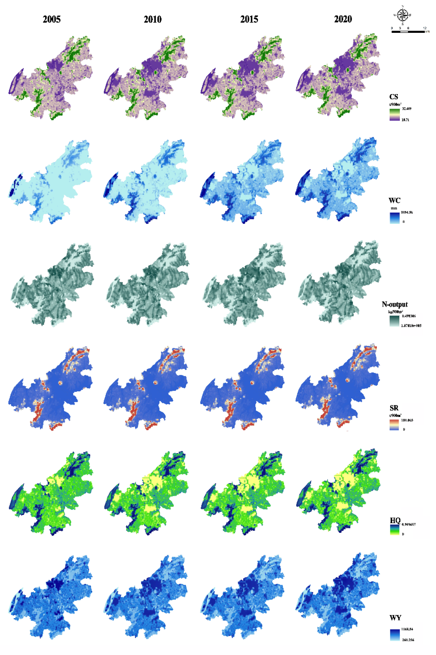
4.1. Spatial and Temporal Patterns of ESs

We assessed the indicators of ESs at both the raster and rural scales using the InVEST model (Figure 3). In terms of the mean values of ESs, the rates of change in the same kinds of ESs were similar at both spatial scales, and the rates of change in ES differed among different kinds of ESs. We found that two metrics (CS and HQ) decreased, and four metrics (N-output, WY, SR, and WR) increased at both scales throughout the study period (2005–2020) (Figure S4). Specifically, CS and HQ continued to decline throughout the study period, whereas WC, SR, and WY increased. The N output increased gradually from 2005 to 2015 and decreased from 2015 to 2020.

From 2005 to 2020, the distribution of ESs in Jiangning showed spatial heterogeneity in terms of spatial patterns at both scales; however, the spatial patterns remained relatively stable. The distribution of ESs formed three types of spatial distribution patterns at the two spatial scales of the grid and rural levels. The high-value areas for CS, WC, SR, and HQ were primarily located in the woodland area of the Tangshan Scenic Area in the north; the woodland areas of Fangshan Park, Niushoushan, and Shogongshan in the centre; the woodland areas of Yuntai Mountain in the southwest; the Hengshan Scenic Area in the south; and along the Yangtze River. The high-value areas of WY were located in the construction land area in central Jiangning, in the area of Lukou Airport in the southeast, and along the Yangtze River around the high-speed railway station at the Jiangning West Station. The patches with high N output values were primarily concentrated in the central part of Jiangning, the Lukou Airport area in the southeast, and the area around the high-speed railway station of Jiangning West Station along the Yangtze River. The remaining areas with high values were scattered in the cultivated land areas in the south and west.

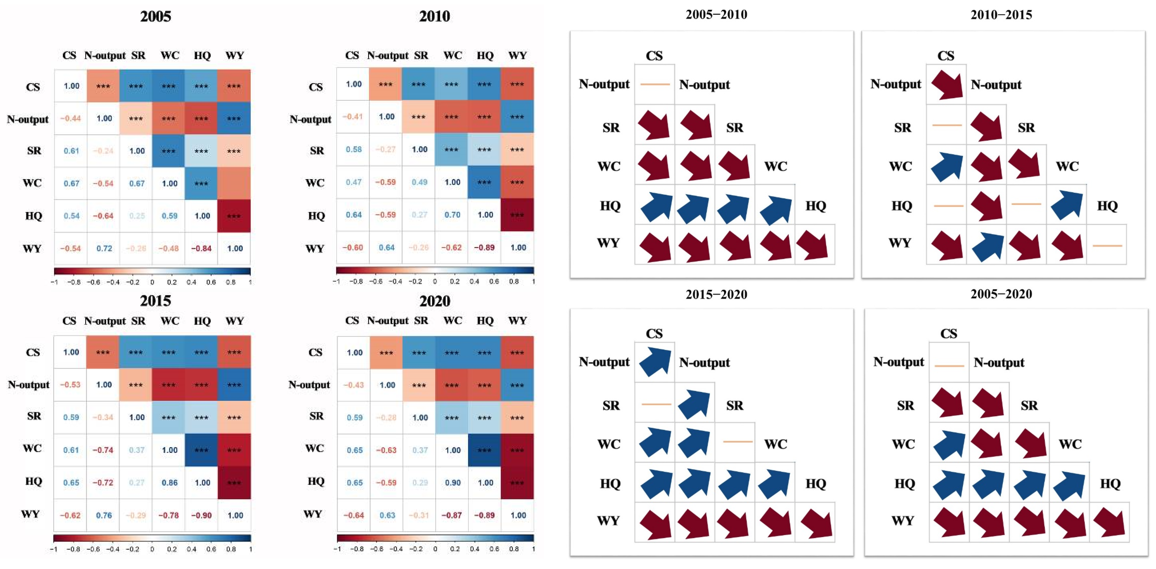
4.2. Spatial and Temporal Correlation between ESs

4.2.1. Correlation Analysis between ESs

Each ES group showed significant correlations (p < 0.05) at both spatial scales and at the raster and rural levels throughout 2005–2020, with 15 correlations identified at each scale for each year (Figure 4 and Figure 5).

As shown in the figure, there were similarities in the correlations between ESs at the two spatial scales over the four years. First, seven positively correlated ES pairs (CS-SR, CS-WC, CS-HQ, N-output-WY, SR-WC, SR-HQ, and WC-HQ) and eight negatively correlated ES pairs were identified. Second, WC-HQ had the highest synergistic ES pairs, whereas HQ-WY had the highest trade-off ES pairs. Third, although there were more trade-off effects between most ES pairs in Jiangning District, synergies increased, and trade-offs decreased between most ES pairs in the 2015–2020 period.

In contrast to the grid scale, at the rural scale, the correlation coefficients exhibited consistently higher absolute values across all four periods; second, the trend of the correlations over the years shows that only five groups of ES pairs (CS-N-output, CS-HQ, N-output-HQ, SR-HQ, and WC-HQ) optimise in the synergistic direction at the grid scale, and at the rural scale, only three groups of ES pairs (CS-HQ, N-output-HQ, SR-HQ) improve.

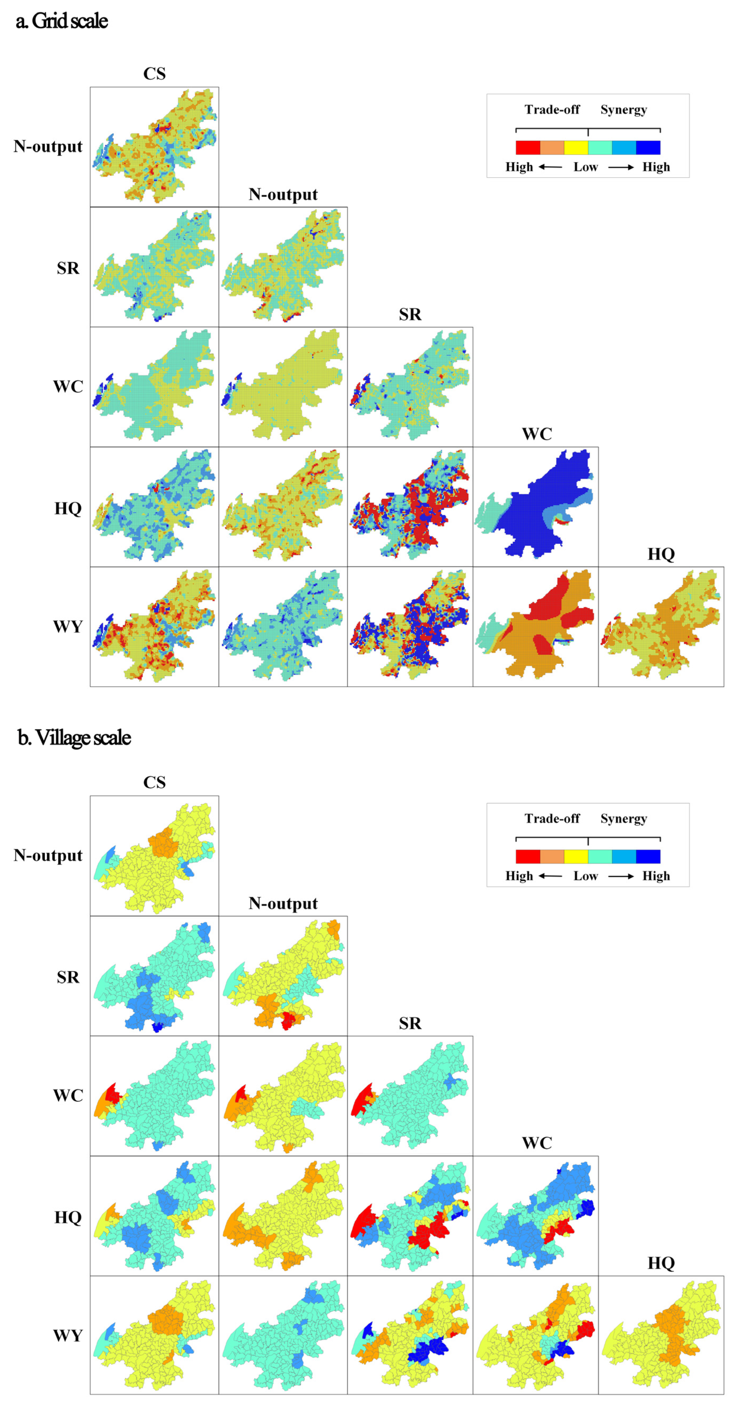
4.2.2. Spatial and Temporal Patterns of Trade-Offs and Synergies among ESs

The GWR regression results showed spatial heterogeneity in the spatial trade-offs and synergistic effects of ES pairs at both raster and rural scales (Figure 6; see Figures S1–S3 in Supplementary Materials).

At the grid scale, spatial synergies were more prevalent than spatial trade-offs for CS-SR, CS-WC, CS-HQ, N-output-WY, SR-WC, SR-HQ, and WC-HQ, and these ES pairs were predominantly spatially synergistic (Figure 7). Significant spatial synergies of these ecosystem services were mainly concentrated in the northern and southern forest margins of Jiangning (CS-SR), along the Yangtze River in the west (CS-WC and SR-WC), and in the Fangshan Mountains in the central part of the country (CS-HQ and SR-HQ).

Similar to the grid scale, the same types of ES pairs with spatial trade-off or spatial synergy characteristics were found at the rural scale, and the same seven pairs of ES were optimised (increase in the area of spatial synergy) at both scales. However, regarding spatial arrangement, ES pairs with high spatial synergistic effects were primarily distributed in the northern and southern forest margins of Jiangning (CS-SR and SR-HQ) and the Fangshan area in the central part of the country (CS-HQ), whereas the high spatial trade-off effect of this column of ES pairs was stronger in the area bordering the Yangtze River. Meanwhile, it is worth noting that the spatial trade-offs and synergistic effects of ES pairs at the rural scale are stronger than those at the grid scale, forming a certain ‘Matthew effect’ of ES pairs.

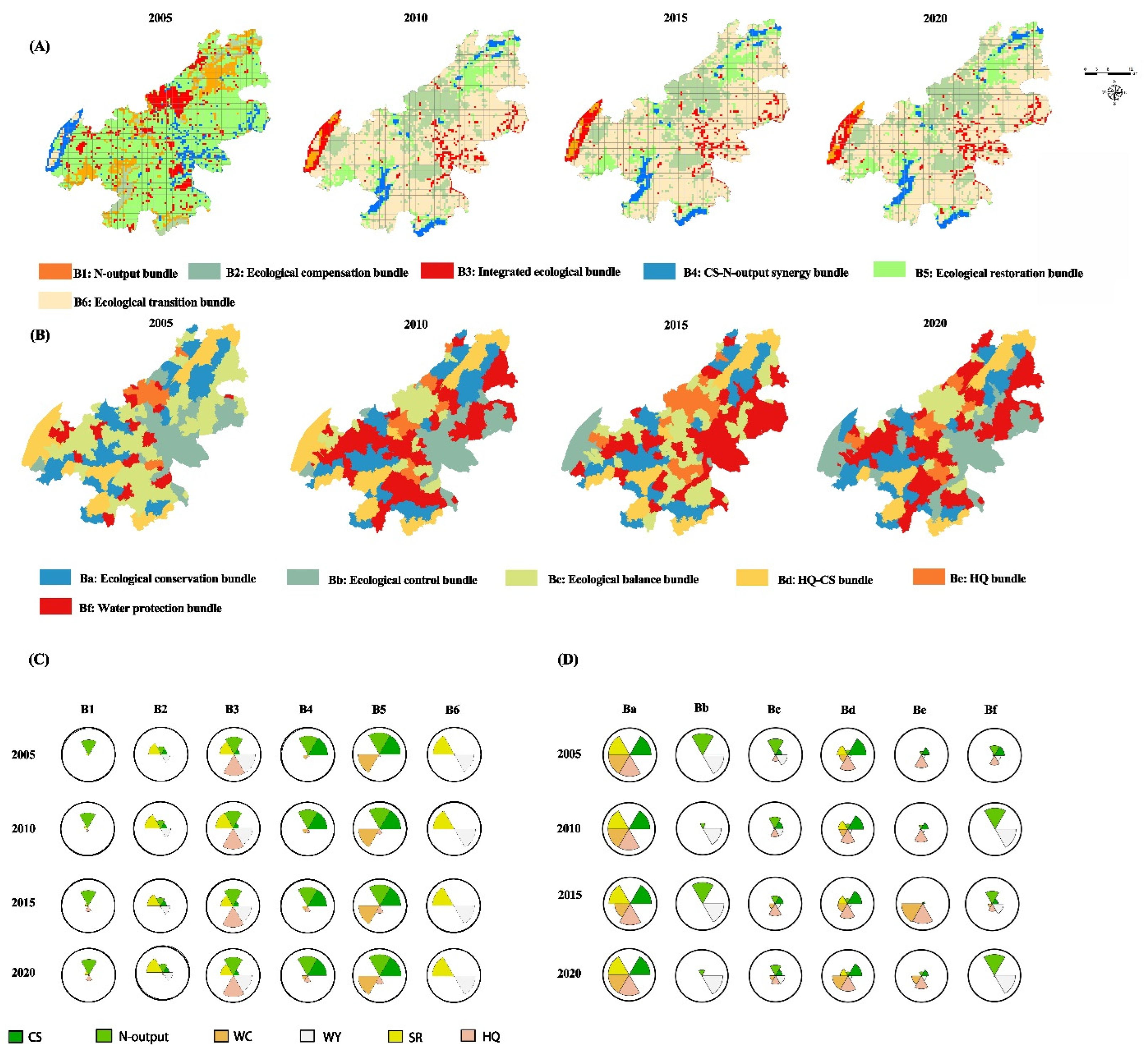
4.3. ES Bundles Spatiotemporal Patterns at Two Scales

Based on the results of the six ES assessments, we used an SOM to identify the six types of ES bundles and their spatial distribution characteristics at both the raster and rural scales in Jiangning for the four periods (Figure 8). Based on the SOM technique, we identified six types of ES beams at village and grid scales. Based on this, we first attempted to name the ES bundle according to its core characteristics. Second, we considered the specific spatial distribution and characteristics of these land use types and finally gave the ES bundle a name based on these three characteristics. Further details on the characteristics of the ES bundles are provided in Supplementary Information S7.

From the perspective of the spatial distribution of ES bundles at the grid and rural scales, we found two essential features: (1) the spatial distribution characteristics of ES bundles in 2005 were different from those of the other years, and (2) the spatial patterns of ES bundles in 2010, 2015, and 2020 were stable and similar, such as the Ba ecological conservation bundle and the Bd HQ-CS bundle, which were located in the north–south forested mountainous terrain.

Meanwhile, by comparing the ES bundles at the raster and rural scales, we found that the emergence of ES bundles was specific to the corresponding scales, for example, N-output bundles, CS-N-output bundles, ecological compensation bundles, integrated ecological bundles at the grid scale, ecological conservation bundles, ecological control bundles, and water protection bundles at the rural scale. Therefore, ES bundles at different scales must be managed according to their objectives and differentiated ES management strategies.

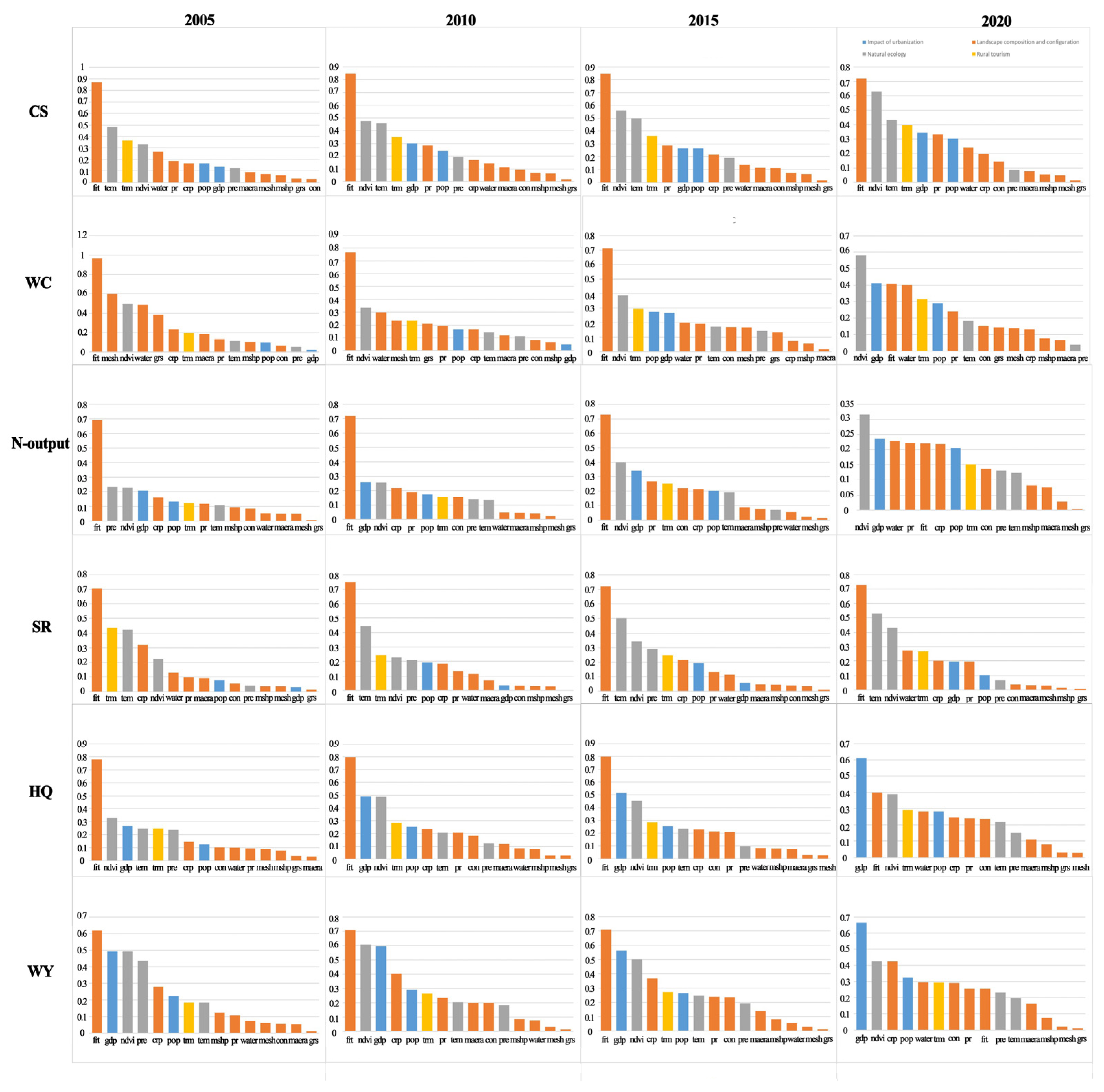
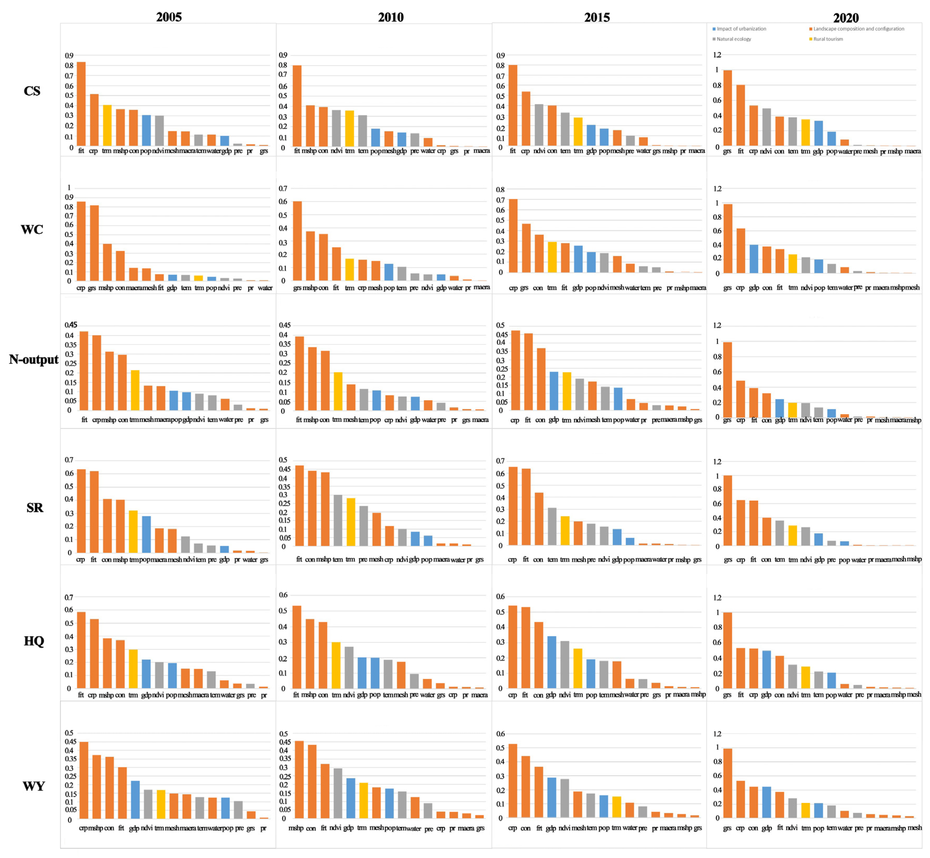
4.4. Social, Ecological, and Landscape Drivers of Ecosystem Services at Multiple Scales and over Multiple Time Periods

We used Geodetector to calculate the influence of social, ecological, and landscape drivers on ecosystem services, identifying the dominant drivers for each type of ES, the extent to which these dominant drivers drive the development of each type of ES, and explore how the dominant drivers change over time and spatial scales (Figure 9 and Figure 10).

The findings are as follows. First, CS was the dominant driver of frt at both rural and grid scales in all periods. In addition, CS was more susceptible to ndvi, tem, and trm at the rural scale than at the grid scale. Meanwhile, it can be found that the influence of frt on CS at the rural scale decreased over time from 2005 to 2020, while the influence of ndvi and trm increased.

Second, WC at the grid scale was primarily driven by crp, mshp, and grs in all periods, and WC at the rural scale was primarily driven by frt, ndvi, and mesh in all periods. Notably, by 2020, gdp became one of the dominant factors for WC at the rural and grid scales.

Third, drivers at the N-output grid scale were primarily frt and crp, with grs added by 2020. During these four periods, frt, ndvi, and gdp were the main drivers at the rural level.

Fourth, during the four periods, the main drivers of the SR at the grid scale were crp, frt, con, meshp, and grs. Among them, meshp had a higher degree of influence in 2005 and 2010; however, its influence decreased significantly in 2015–2020. In contrast, grs had a very low level of influence in 2005–2015, yet it became the main driver in 2020. At the rural scale, the SR continued to be driven by frt and tem. The impact of ndvi increased significantly over time, whereas that of trm decreased significantly.

Fifth, HQ was consistently driven by frt, crp, and con overtime at the grid scale. Similar to the SR, the impact of grs increased dramatically in 2020. Simultaneously, the impact of gdp gradually increased over time.

Sixth, the main drivers of WY at the grid scale were crp, mshp, and con, and, similar to SR, N-output, and HQ, the impact of grs increased dramatically by 2020. The rural scale at different times in WY was consistently affected by drivers frt, gdp, ndvi, pre, and crp.

In summary, we found that the main drivers of each type of ES are different and that the main drivers of the same type of ES can change over time or space. However, it is not difficult to find ES whose main drivers are strong across time and space (e.g., CS), while the main drivers of other ES change with time (e.g., HQ). There are also some ES whose main drivers change with spatial scales (e.g., WC and SR).

5. Discussion

5.1. Spatiotemporal Variation, Interaction Characteristics and Ecological Management Suggestions of ESs

In this study, we quantified the spatial and temporal distributions of ESs from 2005 to 2020 with an accuracy of 30 m, which is essential for improving the accuracy of the InVEST model data [45]. Compared to our previous research [79], this is an important reason why we increased the resolution to 30 m in this study. We found that the spatial and temporal variations in WC, SR, and WY in Jiangning increased significantly from 2005 to 2020, the spatial patterns of CS, WC, SR, and HQ were similar, and the areas with more ESs were concentrated in forested, hilly, and riparian areas of the mountainous region, which is due to the fact that these areas have a continuous wide range of forested landscapes and riparian landscapes, which have beautiful ecological environments and a low degree of habitat fragmentation and are suitable for the growth of plants and animals, which can provide a carbon sink and a riverbank growth, and can provide carbon sinks and complete habitats [22,80]. Forests exhibit a stable soil structure, and their canopy effectively mitigates the impact of rainfall on soil [81,82]. The spatial distribution of high SRs in our results is consistent with this finding. In addition, the higher elevation and diverse topography of these regions contribute to humid airflow, leading to abundant precipitation, whereas high elevations also lead to lower evapotranspiration. The riparian region has a unique water resource capacity owing to its reliance on the Yangtze River; therefore, all these topographic and climatic features promote the water-holding capacity and conservation potential of the region [22]. Moreover, the total CS and HQ at both the raster and rural scales decreased, whereas the total amount of N-output gradually increased from 2005 to 2015 and decreased from 2015 to 2020. Therefore, based on the temporal and spatial patterns of ESs, managers and planners should focus on improving the capacity for ESs, carbon storage, and habitat quality in the future.

This study also explains the interactions between ESs in the Jiangning region from 2005 to 2020. In general, there is a trade-off between N output and other ESs, which is consistent with the results of a study in Anhui Province [83]. This finding sets priorities for ES management in Jiangning. Future efforts should first focus on addressing nitrogen output trade-offs to mitigate the degradation of natural ecosystems caused by integrated rural development.

On a dynamic time scale, we also conducted a study on the spatial interaction correlation of ESs over time in Jiangning District and found that the synergistic effects of CS-WC, N-output-WY, and SR-WC decreased at the grid and rural scales between 2005 and 2020 (Figure 4 and Figure 5). The synergistic effects of the spatial trade-offs of the three types of ES pairs at the grid and rural scales (CS-WC, N output-WY, and SR-WC) increased while spatial synergies decreased. The reduced synergies in the ES pairs linked to WC or WY may be associated with climatic uncertainties, including precipitation [22,84,85]. Notably, we found synergistic ecological protection bundles (Ba) and CS-WC synergistic ecological restoration bundles (B5) at the rural scale. As the synergistic relationship between CS-SR and CS-WC showed degradation in spatial and temporal analyses, we addressed the need to improve the ecosystem coping with GHG emissions in ES bundles at the corresponding scales to address this issue, extreme precipitation, and climate change resilience. This suggests the importance of integrating spatial and temporal analyses of ecosystem service interactions into spatial planning [22].

In addition, in terms of the spatial interaction correlation of ESs, there is a ‘Matthew effect’ in the spatial trade-offs and synergies of ESs. We found that the spatial trade-off or spatial synergistic effects of rural-scale ESs were stronger than those of raster-scale ESs and that there was a tendency for high trade-off/high synergistic and low trade-off/low synergistic ratios to be clustered (Figure 7). Combined with other studies [86] and the characteristics of this study, the ‘Matthew effect’ referred to in this study means that large-scale, high-trade-off or high-synergy ecosystem service areas are more likely to induce stronger feedback effects, thus strengthening the trade-off or synergy between ecosystem services. For example, the area that leads to high regional trade-off or high coordination is wider, that is, the ‘Matthew effect’ is displayed. Therefore, it is required to strengthen the existing ES advantage areas in the optimisation strategy, that is, to give full play to the advantages of ‘the stronger’ areas and strengthen the ecological management strategy at the village level so as to achieve the effect of high ecological return on small economic investment and maximise the comprehensive benefits of ecological improvement.

5.2. ES Bundles, Social Drivers, and Optimisation Strategy Guidelines

The accurate identification of social, ecological, and landscape drivers across spatial scales is essential for the human manipulation of social, ecological, and landscape drivers to manage multiple ESs simultaneously, improve geospatial multifunctionality, and promote sustainable regional development [22].

Based on the various research results, this study proposes corresponding strategies and suggestions for rural planning optimisation, which are listed below.

We found that the relationship between CS and drivers was stronger at both scales, and woodland and grassland were the main influencing factors, which suggests the significance of landscape measures, such as afforestation, reduction in bare ground, and an increase in the amount of vegetation, for CS enhancement at both scales [87].

Additionally, the proportions of forest, NDVI, and tourism had significant effects on the amount of CS and SR (Figure 9 and Figure 10). Based on these results, this study proposes two planning optimisation strategies: (1) planning and improvement should be carried out from the perspective of forest protection, moderate natural afforestation, control of urban expansion, and protection of farmland ecosystems, which can specifically increase woodland area and improve the function of forest ecosystems.

At the same time, afforestation or planting grass on bare land should be considered to increase the vegetation coverage and complexity of the vegetation level, thereby increasing the stability of the soil and strengthening the protection and restoration of vegetation. It is also necessary to add trees and build buffer zones, such as forest belts in the periphery of farmlands, which can effectively filter fertiliser pollution, control the expansion of construction land, and encourage the implementation of diversified ecological agriculture planting patterns such as crop rotation and intercropping, planting cover crops in non-growing season, reducing soil erosion, and improving soil fertility and carbon storage capacity.

Moreover, agricultural waste can be converted into organic fertiliser or energy, reducing the environmental impact of waste and increasing soil organic matter and carbon storage. (2) It is necessary to build a park ecological network for rural tourism in Jiangning, appropriately develop natural landscape resources according to the carrying capacity of regional resources and the environment, increase the construction of parks in various villages, and develop ecotourism and leisure agriculture simultaneously. Through the multi-functional utilisation of farmland, economic benefits are increased, farmland ecosystems are protected and restored, and the problem of rural ecological environment deterioration is artificially solved.

Furthermore, it is worth noting that some indicators of landscape structure and composition (e.g., con, mshp, and grass proportion) have a greater impact at the grid scale than at the rural scale, which can be attributed to the fact that subtle landscape configurations can be better captured at smaller scales. Therefore, the targeted improvement of rural landscape space design needs to focus on the refinement of the 500 m spatial scale and achieve the bare ground, unused land ‘500 m to see green’ and landscape design supplementation and refinement, and this step of optimisation needs to be supported by land consolidation, which is an effective tool to reduce land fragmentation and optimise land use structure [22].

More importantly, tourism parks have a greater impact on the rural scale than on the grid. This implies that creating ecotourism through landscape planning and building parks on a rural scale is effective in enhancing overall ecological service effectiveness at the rural level [88]. These strategies are crucial for the sustainable development of the ecological protection bundles (Ba), ecological control bundles (Bb), ecological compensation (B2), and integrated ecological bundles (B3).

5.3. Significance of Rural Planning Optimisation Strategy Based on ESs

As a typical example of rural revitalisation, Jiangning is at the forefront of China’s rural areas in terms of its level of comprehensive rural development, including rural governance, rural construction, and rural tourism. However, there is still a need to promote ecological construction to mitigate the ecological threats that continue to be posed by urbanisation, rural modernisation, and construction.

Previous studies have demonstrated that it is unreasonable to use alternative governance at spatial scales that do not correspond to them, owing to the possibility that different scales do not necessarily produce similar distributions of ESs, trade-offs/synergistic relationships, or ES bundles [48,62,88].

Currently, studies based on ESs for spatial planning in rural landscapes remain uncommon. However, they can further identify refined planning, differentiated interventions, and policy formulation, particularly at fine-grid scales. By providing spatial planning and guidance at both rural and grid scales, this study provides hierarchical spatial planning and management policy recommendations for rural landscapes and provides comprehensive, precise, and detailed spatial optimisation strategies for rural spaces, contributing to the revitalisation of rural areas from ecological and landscape disciplinary aspects. The main significance of this study at a practical level is as follows:

First, to maintain the sustainability of rural ecology and reduce the degradation of the ecological environment, it is necessary to increase the area of natural afforestation at the rural scale and to manage and prevent water pollution in key watersheds because the trade-offs and synergistic effects among ESs at the rural scale have a greater ‘Matthew effect’, which indicates that this spatial scale has a higher potential for the management of different ESs and that it is more suitable for the development of the rural area. Enhancement at this scale can improve ecosystems more rapidly and holistically and can have an immediate effect on the overall effectiveness of regional ESs [48].

Furthermore, compared with smaller ecological scales, the administrative level at the rural scale is often more suitable for governmental decision-making and management, as well as for the development and implementation of landscape spatial planning [16]. Therefore, the overall tone of spatial planning and ecological management should be set at this level.

Second, ecological optimisation at the grid-scale level was carried out through landscape measures to improve the refinement of the 500 m spatial scale of the rural landscape. This is because the grid scale is the most sensitive to the response of landscape drivers; therefore, a refined landscape design within the grid 500 m scale is more effective for the precise enhancement of ESs. Therefore, planning and landscape design strategies for raster units can be formulated based on the results at the rural scale in conjunction with ecological units [16].

Third, considering the spatial pattern of different ecosystem services comprehensively, we found that the ES spatial pattern distribution at different scales was relatively stable, which is consistent with the results of other studies [22].

5.4. Limitations

This study provides information on ESs and their relationships with social, ecological, and landscape drivers at different scales in the rural areas of Jiangning. It offers specific recommendations for hierarchical spatial planning and landscape management in urban–rural integrated rural areas, as well as a prior reference for other rural areas developed under the rural revitalisation goal.

However, there are some limitations in this study: (1) the selection of six ESs and fifteen social, ecological, and landscape drivers for rural areas in Jiangning is limited by data availability, which may potentially affect our study, and the inclusion of more ESs and drivers for a more comprehensive analysis is a part of the future need for improvement; and (2) with the change in time, the effect of drivers on the different ESs will also change. This study only analysed ESs and drivers for 2020, and future work can further explore the relationship between ESs and drivers for different time periods.

Despite these limitations, the results of this study are relevant. By incorporating ESs into rural spatial planning and ecological governance, we provide a bridge to how land can be used more efficiently in current rural landscape practices. The results of this study can help planning and landscape practitioners and governments comprehensively consider the social, ecological, and landscape drivers of ESs, which are important for enhancing rural ESs and thus promoting rural revitalisation from an ecological and landscape perspective.

6. Conclusions

To utilise the knowledge of ESs more deeply for ecological management and landscape planning in rural areas, this study investigates land use changes in the Jiangning area, a rural area in the metropolitan fringe region, from 2005 to 2020, with different spatial and temporal scales of six ESs: spatial and temporal distributions of ESs, interactions among ESs (trade-offs and synergisms), and the distribution of ES bundles. It also explores the social, ecological, and landscape drivers that are of fundamental significance for achieving the sustainable development of suburban rural areas and targeting the optimisation and enhancement of rural spaces.

First, over the study period, the predominant form of land expansion in rural Jiangning involved construction land, marking a 74% increase, predominantly transitioning from cropland and forest land to construction land.

Second, mapping the six ecosystem services uncovered spatial heterogeneity in their distribution. HQ experienced the most significant decline, dropping by 11.288% at the grid scale and experiencing a decrease of 14.53% at the rural scale.

Third, the trade-off effect among ES pairs dominated throughout the study period in the rural areas of Jiangning (eight ES pairs with trade-off effects and seven ES pairs with synergistic effects); five groups of ES (CS-N-output, CS-HQ, N-output-HQ, SR-HQ, and WC-HQ) pairs optimised in the synergistic direction at the grid scale and there are only three ES pairs (CS-HQ, N-output-HQ, and SR-HQ) at the rural scale; the effect of scale on the direction of trade-offs and synergies between ESs does not change, but the intensity and spatial extent change. We identify that the trade-off effects are mainly between N-output and other ES trade-offs and prioritise the management of ESs.

Fourth, the spatial scale effect of ESs exists in suburban rural areas; a ‘Matthew effect’ is evident in the spatial trade-offs and synergistic effects of ecosystem services. Notably, we observed that the trade-offs or synergies among ecosystem service pairs were more pronounced at the rural scale than at the grid scale, which emphasises the importance of prioritising the improvement and upgrading of trade-off ES pairs.

Fifth, we identify the major trade-offs of ES pairs and classify ES bundles based on the distributional characteristics of the ES bundles and spatiotemporal analyses of the ES pairs, which is a key element of our ecosystem service multi-scale hierarchical management.

Finally, by analysing drivers across different scales for commonalities and distinctions, we determined the connections and priorities for spatial planning at various levels. Subsequently, we propose hierarchical spatial planning and landscape policies for rural landscapes, addressing two spatial scales: administrative and fine.

Fundamentally, by optimising rural landscape planning and ecological management to enhance the overall ecological effectiveness of rural areas, we contribute to rural revitalisation in the ecological and landscape disciplines.

References

1. Yang, H. Review on the Development Process of Rural Landscape Practice in China (1949–2022). Landsc. Archit. Acad. J. 2022, 39, 10–17. [Google Scholar]
2. Bhatta, L.D.; van Oort, B.E.H.; Stork, N.E.; Baral, H. Ecosystem services and livelihoods in a changing climate: Understanding local adaptations in the Upper Koshi, Nepal. Int. J. Biodivers. Sci. Ecosyst. Serv. Manag. 2015, 11, 145–155. [Google Scholar] [CrossRef]
3. Bai, Y.; Zhuang, C.; Ouyang, Z.; Zheng, H.; Jiang, B. Spatial characteristics between biodiversity and ecosystem services in a human-dominated watershed. Ecol. Complex. 2011, 8, 177–183. [Google Scholar] [CrossRef]
4. Costanza, R.; d’Arge, R.; De Groot, R.; Farber, S.; Grasso, M.; Hannon, B.; Limburg, K.; Naeem, S.; O’Neill, R.V.; Paruelo, J.; et al. The value of the world’s ecosystem services and natural capital. Nature 1997, 387, 253–260. [Google Scholar] [CrossRef]
5. Millennium Ecosystem Assessment. Ecosystems and Human Well-Being; Island Press: Washington, DC, USA, 2005. [Google Scholar]
6. De Groot, R.; Brander, L.; Van Der Ploeg, S.; Costanza, R.; Bernard, F.; Braat, L.; Christie, M.; Crossman, N.; Ghermandi, A.; Hein, L.; et al. Global estimates of the value of ecosystems and their services in monetary units. Ecosyst. Serv. 2012, 1, 50–61. [Google Scholar] [CrossRef]
7. Wong, C.P.; Jiang, B.; Kinzig, A.P.; Lee, K.N.; Ouyang, Z. Linking ecosystem characteristics to final ecosystem services for public policy. Ecol. Lett. 2015, 18, 108–118. [Google Scholar] [CrossRef] [PubMed]
8. Li, J.; Bai, Y.; Alatalo, J.M. Impacts of rural tourism-driven land use change on ecosystems services provision in Erhai Lake Basin, China. Ecosyst. Serv. 2020, 42, 101081. [Google Scholar] [CrossRef]
9. Yang, M.; Gao, X.; Zhao, X.; Wu, P. Scale effect and spatially explicit drivers of interactions between ecosystem services—A case study from the Loess Plateau. Sci. Total Environ. 2021, 785, 147389. [Google Scholar] [CrossRef]
10. Guerry, A.D.; Polasky, S.; Lubchenco, J.; Chaplin-Kramer, R.; Daily, G.C.; Griffin, R.; Ruckelshaus, M.; Bateman, I.J.; Duraiappah, A.; Elmqvist, T.; et al. Natural capital and ecosystem services informing decisions: From promise to practice. Proc. Natl. Acad. Sci. USA 2015, 112, 7348–7355. [Google Scholar] [CrossRef] [PubMed]
11. Ouyang, Z.; Zheng, H.; Xiao, Y.; Polasky, S.; Liu, J.; Xu, W.; Wang, Q.; Zhang, L.; Xiao, Y.; Rao, E.; et al. Improvements in ecosystem services from investments in natural capital. Science 2016, 352, 1455–1459. [Google Scholar] [CrossRef]
12. Andersson, E.; McPhearson, T.; Kremer, P.; Gomez-Baggethun, E.; Haase, D.; Tuvendal, M.; Wurster, D. Scale and context dependence of ecosystem service providing units. Ecosyst. Serv. 2015, 12, 157–164. [Google Scholar] [CrossRef]
13. Dade, M.C.; Mitchell, M.G.; McAlpine, C.A.; Rhodes, J.R. Assessing ecosystem service trade-offs and synergies: The need for a more mechanistic approach. Ambio 2019, 48, 1116–1128. [Google Scholar] [CrossRef] [PubMed]
14. Falk, T.; Spangenberg, J.H.; Siegmund-Schultze, M.; Kobbe, S.; Feike, T.; Kuebler, D.; Settele, J.; Vorlaufer, T. Identifying governance challenges in ecosystem services management–Conceptual considerations and comparison of global forest cases. Ecosyst. Serv. 2018, 32, 193–203. [Google Scholar] [CrossRef]
15. Ndong, G.O.; Therond, O.; Cousin, I. Analysis of relationships between ecosystem services: A generic classification and review of the literature. Ecosyst. Serv. 2020, 43, 101120. [Google Scholar] [CrossRef]
16. Chen, H.; Yan, W.; Li, Z.; Wende, W.; Xiao, S.; Wan, S.; Li, S. Spatial patterns of associations among ecosystem services across different spatial scales in metropolitan areas: A case study of Shanghai, China. Ecol. Indic. 2022, 136, 108682. [Google Scholar] [CrossRef]
17. Keeler, B.L.; Dalzell, B.J.; Gourevitch, J.D.; Hawthorne, P.L.; Johnson, K.A.; Noe, R.R. Putting people on the map improves the prioritization of ecosystem services. Front. Ecol. Environ. 2019, 17, 151–156. [Google Scholar] [CrossRef]
18. Gong, J.; Jin, T.; Liu, D.; Zhu, Y.; Yan, L. Are ecosystem service bundles useful for mountainous landscape function zoning and management? A case study of Bailongjiang watershed in western China. Ecol. Indic. 2022, 134, 108495. [Google Scholar] [CrossRef]
19. Liu, H.; Hu, Y.; Li, F.; Yuan, L. Associations of multiple ecosystem services and disservices of urban park ecological infrastructure and the linkages with socioeconomic factors. J. Clean. Prod. 2018, 174, 868–879. [Google Scholar] [CrossRef]
20. Zhang, Z.; Liu, Y.; Wang, Y.; Liu, Y.; Zhang, Y.; Zhang, Y. What factors affect the synergy and tradeoff between ecosystem services, and how, from a geospatial perspective? J. Clean. Prod. 2020, 257, 120454. [Google Scholar] [CrossRef]
21. Xu, J.; Wang, S.; Xiao, Y.; Xie, G.; Wang, Y.; Zhang, C.; Li, P.; Lei, G. Mapping the spatiotemporal heterogeneity of ecosystem service relationships and bundles in Ningxia, China. J. Clean. Prod. 2021, 294, 126216. [Google Scholar] [CrossRef]
22. Xia, H.; Yuan, S.; Prishchepov, A.V. Spatial-temporal heterogeneity of ecosystem service interactions and their social-ecological drivers: Implications for spatial planning and management. Resour. Conserv. Recycl. 2023, 189, 106767. [Google Scholar] [CrossRef]
23. Mouchet, M.A.; Lamarque, P.; Martín-López, B.; Crouzat, E.; Gos, P.; Byczek, C.; Lavorel, S. An interdisciplinary methodological guide for quantifying associations between ecosystem services. Glob. Environ. Change 2014, 28, 298–308. [Google Scholar] [CrossRef]
24. Mach, M.E.; Martone, R.G.; Chan, K.M. Human impacts and ecosystem services: Insufficient research for trade-off evaluation. Ecosyst. Serv. 2015, 16, 112–120. [Google Scholar] [CrossRef]
25. Spake, R.; Lasseur, R.; Crouzat, E.; Bullock, J.M.; Lavorel, S.; Parks, K.E.; Schaafsma, M.; Bennett, E.M.; Maes, J.; Mulligan, M.; et al. Unpacking ecosystem service bundles: Towards predictive mapping of synergies and trade-offs between ecosystem services. Glob. Environ. Change 2017, 47, 37–50. [Google Scholar] [CrossRef]
26. Grêt-Regamey, A.; Altwegg, J.; Sirén, E.A.; Van Strien, M.J.; Weibel, B. Integrating ecosystem services into spatial planning—A spatial decision support tool. Landsc. Urban Plan. 2017, 165, 206–219. [Google Scholar] [CrossRef]
27. Xu, L.-X.; Yang, D.-W.; Wu, T.-H.; Yi, S.-H.; Fang, Y.-P.; Xiao, C.-D.; Lin, H.-X.; Huang, J.-C.; Simbi, C.H. An ecosystem services zoning framework for the permafrost regions of China. Adv. Clim. Change Res. 2019, 10, 92–98. [Google Scholar] [CrossRef]
28. Raudsepp-Hearne, C.; Peterson, G.D.; Bennett, E.M. Ecosystem service bundles for analyzing tradeoffs in diverse landscapes. Proc. Natl. Acad. Sci. USA 2010, 107, 5242–5247. [Google Scholar] [CrossRef] [PubMed]
29. Kareiva, P.; Watts, S.; McDonald, R.; Boucher, T. Domesticated nature: Shaping landscapes and ecosystems for human welfare. Science 2007, 316, 1866–1869. [Google Scholar] [CrossRef] [PubMed]
30. Bennett, E.M.; Peterson, G.D.; Gordon, L.J. Understanding relationships among multiple ecosystem services. Ecol. Lett. 2009, 12, 1394–1404. [Google Scholar] [CrossRef] [PubMed]
31. Crouzat, E.; Mouchet, M.; Turkelboom, F.; Byczek, C.; Meersmans, J.; Berger, F.; Verkerk, P.J.; Lavorel, S. Assessing bundles of ecosystem services from regional to landscape scale: Insights from the French Alps. J. Appl. Ecol. 2015, 52, 1145–1155. [Google Scholar] [CrossRef]
32. Felipe-Lucia, M.R.; Soliveres, S.; Penone, C.; Manning, P.; van der Plas, F.; Boch, S.; Prati, D.; Ammer, C.; Schall, P.; Gossner, M.M.; et al. Multiple forest attributes underpin the supply of multiple ecosystem services. Nat. Commun. 2018, 9, 4839. [Google Scholar] [CrossRef] [PubMed]
33. Zhang, M.; Wang, K.; Liu, H.; Zhang, C.; Yue, Y.; Qi, X. Effect of ecological engineering projects on ecosystem services in a karst region: A case study of northwest Guangxi, China. J. Clean. Prod. 2018, 183, 831–842. [Google Scholar] [CrossRef]
34. Wilkerson, M.L.; Mitchell, M.G.; Shanahan, D.; Wilson, K.A.; Ives, C.D.; Lovelock, C.E.; Rhodes, J.R. The role of socio-economic factors in planning and managing urban ecosystem services. Ecosyst. Serv. 2018, 31, 102–110. [Google Scholar] [CrossRef]
35. Xu, J.; Chen, J.; Liu, Y.; Fan, F. Identification of the geographical factors influencing the relationships between ecosystem services in the Belt and Road region from 2010 to 2030. J. Clean. Prod. 2020, 275, 124153. [Google Scholar] [CrossRef]
36. Bai, Y.; Chen, Y.; Alatalo, J.M.; Yang, Z.; Jiang, B. Scale effects on the relationships between land characteristics and ecosystem services-a case study in Taihu Lake Basin, China. Sci. Total Environ. 2020, 716, 137083. [Google Scholar] [CrossRef] [PubMed]
37. Huang, A.; Xu, Y.; Sun, P.; Zhou, G.; Liu, C.; Lu, L.; Xiang, Y.; Wang, H. Land use/land cover changes and its impact on ecosystem services in ecologically fragile zone: A case study of Zhangjiakou City, Hebei Province, China. Ecol. Indic. 2019, 104, 604–614. [Google Scholar] [CrossRef]
38. Wang, R.; Bai, Y.; Alatalo, J.M.; Yang, Z.; Yang, Z.; Yang, W.; Guo, G. Impacts of rapid urbanization on ecosystem services under different scenarios—A case study in Dianchi Lake Basin, China. Ecol. Indic. 2021, 130, 108102. [Google Scholar] [CrossRef]
39. Raudsepp-Hearne, C.; Peterson, G.D. Scale and ecosystem services: How do observation, management, and analysis shift with scale—Lessons from Québec. Ecol. Soc. 2016, 21, 16. [Google Scholar] [CrossRef]
40. Sannigrahi, S.; Zhang, Q.; Joshi, P.; Sutton, P.C.; Keesstra, S.; Roy, P.; Pilla, F.; Basu, B.; Wang, Y.; Jha, S.; et al. Examining effects of climate change and land use dynamic on biophysical and economic values of ecosystem services of a natural reserve region. J. Clean. Prod. 2020, 257, 120424. [Google Scholar] [CrossRef]
41. Wang, Y.; Dai, E. Spatial-temporal changes in ecosystem services and the trade-off relationship in mountain regions: A case study of Hengduan Mountain region in Southwest China. J. Clean. Prod. 2020, 264, 121573. [Google Scholar] [CrossRef]
42. Mehring, M.; Ott, E.; Hummel, D. Ecosystem services supply and demand assessment: Why social-ecological dynamics matter. Ecosyst. Serv. 2018, 30, 124–125. [Google Scholar] [CrossRef]
43. Sun, X.; Wu, J.; Tang, H.; Yang, P. An urban hierarchy-based approach integrating ecosystem services into multiscale sustainable land use planning: The case of China. Resour. Conserv. Recycl. 2022, 178, 106097. [Google Scholar] [CrossRef]
44. Moreno-Llorca, R.; Vaz, A.; Herrero, J.; Millares, A.; Bonet-García, F.; Alcaraz-Segura, D. Multi-scale evolution of ecosystem services’ supply in Sierra Nevada (Spain): An assessment over the last half-century. Ecosyst. Serv. 2020, 46, 101204. [Google Scholar] [CrossRef]
45. Liu, L.; Wu, J. Ecosystem services-human wellbeing relationships vary with spatial scales and indicators: The case of China. Resour. Conserv. Recycl. 2021, 172, 105662. [Google Scholar] [CrossRef]
46. Scholes, R.J.; Reyers, B.; Biggs, R.; Spierenburg, M.; Duriappah, A. Multi-scale and cross-scale assessments of social–ecological systems and their ecosystem services. Curr. Opin. Environ. Sustain. 2013, 5, 16–25. [Google Scholar] [CrossRef]
47. Steur, G.; Verburg, R.W.; Wassen, M.J.; Verweij, P.A. Shedding light on relationships between plant diversity and tropical forest ecosystem services across spatial scales and plot sizes. Ecosyst. Serv. 2020, 43, 101107. [Google Scholar] [CrossRef]
48. Shen, J.; Li, S.; Liu, L.; Liang, Z.; Wang, Y.; Wang, H.; Wu, S. Uncovering the relationships between ecosystem services and social-ecological drivers at different spatial scales in the Beijing-Tianjin-Hebei region. J. Clean. Prod. 2021, 290, 125193. [Google Scholar] [CrossRef]
49. Emmett, B.A.; Cooper, D.; Smart, S.; Jackson, B.; Thomas, A.; Cosby, B.; Evans, C.; Glanville, H.; McDonald, J.E.; Malham, S.K.; et al. Spatial patterns and environmental constraints on ecosystem services at a catchment scale. Sci. Total Environ. 2016, 572, 1586–1600. [Google Scholar] [CrossRef] [PubMed]
50. Hou, Y.; Lü, Y.; Chen, W.; Fu, B. Temporal variation and spatial scale dependency of ecosystem service interactions: A case study on the central Loess Plateau of China. Landsc. Ecol. 2017, 32, 1201–1217. [Google Scholar] [CrossRef]
51. Pan, J.; Wei, S.; Li, Z. Spatiotemporal pattern of trade-offs and synergistic relationships among multiple ecosystem services in an arid inland river basin in NW China. Ecol. Indic. 2020, 114, 106345. [Google Scholar] [CrossRef]
52. Bai, Y.; Wong, C.P.; Jiang, B.; Hughes, A.C.; Wang, M.; Wang, Q. Developing China’s Ecological Redline Policy using ecosystem services assessments for land use planning. Nat. Commun. 2018, 9, 3034. [Google Scholar] [CrossRef] [PubMed]
53. Wang, S.; Hu, M.; Wang, Y.; Xia, B. Dynamics of ecosystem services in response to urbanization across temporal and spatial scales in a mega metropolitan area. Sustain. Cities Soc. 2022, 77, 103561. [Google Scholar] [CrossRef]
54. Xue, S.; Fang, Z.; Bai, Y.; Alatalo, J.M.; Yang, Y.; Zhang, F. The next step for China’s national park management: Integrating ecosystem services into space boundary delimitation. J. Environ. Manag. 2023, 329, 117086. [Google Scholar] [CrossRef] [PubMed]
55. Villa, F.; Voigt, B.; Erickson, J.D. New perspectives in ecosystem services science as instruments to understand environmental securities. Philos. Trans. R. Soc. B Biol. Sci. 2014, 369, 20120286. [Google Scholar] [CrossRef] [PubMed]
56. Liu, Y.; Li, T.; Zhao, W.; Wang, S.; Fu, B. Landscape functional zoning at a county level based on ecosystem services bundle: Methods comparison and management indication. J. Environ. Manag. 2019, 249, 109315. [Google Scholar] [CrossRef] [PubMed]
57. Zheng, D.; Wang, Y.; Hao, S.; Xu, W.; Lv, L.; Yu, S. Spatial-temporal variation and tradeoffs/synergies analysis on multiple ecosystem services: A case study in the Three-River Headwaters region of China. Ecol. Indic. 2020, 116, 106494. [Google Scholar] [CrossRef]
58. Peng, J.; Wang, A.; Luo, L.; Liu, Y.; Li, H.; Hu, Y.n.; Meersmans, J.; Wu, J. Spatial identification of conservation priority areas for urban ecological land: An approach based on water ecosystem services. Land Degrad. Dev. 2019, 30, 683–694. [Google Scholar] [CrossRef]
59. Gebre, T.; Gebremedhin, B. The mutual benefits of promoting rural-urban interdependence through linked ecosystem services. Glob. Ecol. Conserv. 2019, 20, e00707. [Google Scholar] [CrossRef]
60. Chen, J.; Jiang, B.; Bai, Y.; Xu, X.; Alatalo, J.M. Quantifying ecosystem services supply and demand shortfalls and mismatches for management optimisation. Sci. Total Environ. 2019, 650, 1426–1439. [Google Scholar] [CrossRef] [PubMed]
61. Sharp, R.; Tallis, H.; Ricketts, T.; Guerry, A.D.; Wood, S.A.; Chaplin-Kramer, R.; Nelson, E.; Ennaanay, D.; Wolny, S.; Olwero, N.; et al. InVEST+ VERSION+ User’s Guide; The Natural Capital Project, Stanford University: Stanford, CA, USA, 2016. [Google Scholar]
62. Qiu, J.; Carpenter, S.R.; Booth, E.G.; Motew, M.; Zipper, S.C.; Kucharik, C.J.; Loheide, S.P., II; Turner, M.G. Understanding relationships among ecosystem services across spatial scales and over time. Environ. Res. Lett. 2018, 13, 054020. [Google Scholar] [CrossRef]
63. Xu, H.-j.; Zhao, C.-y.; Chen, S.-y.; Shan, S.-y.; Qi, X.-l.; Chen, T.; Wang, X.-p. Spatial relationships among regulating ecosystem services in mountainous regions: Nonlinear and elevation-dependent. J. Clean. Prod. 2022, 380, 135050. [Google Scholar] [CrossRef]
64. Brunsdon, C.; Fotheringham, A.S.; Charlton, M.E. Geographically weighted regression: A method for exploring spatial nonstationarity. Geogr. Anal. 1996, 28, 281–298. [Google Scholar] [CrossRef]
65. Chen, S.; Feng, Y.; Tong, X.; Liu, S.; Xie, H.; Gao, C.; Lei, Z. Modeling ESV losses caused by urban expansion using cellular automata and geographically weighted regression. Sci. Total Environ. 2020, 712, 136509. [Google Scholar] [CrossRef] [PubMed]
66. Wang, X.; Wu, J.; Liu, Y.; Hai, X.; Shanguan, Z.; Deng, L. Driving factors of ecosystem services and their spatiotemporal change assessment based on land use types in the Loess Plateau. J. Environ. Manag. 2022, 311, 114835. [Google Scholar] [CrossRef] [PubMed]
67. Foody, G. Geographical weighting as a further refinement to regression modelling: An example focused on the NDVI–rainfall relationship. Remote Sens. Environ. 2003, 88, 283–293. [Google Scholar] [CrossRef]
68. Oshan, T.M.; Smith, J.P.; Fotheringham, A.S. Targeting the spatial context of obesity determinants via multiscale geographically weighted regression. Int. J. Health Geogr. 2020, 19, 11. [Google Scholar] [CrossRef]
69. Zhu, C.; Zhang, X.; Zhou, M.; He, S.; Gan, M.; Yang, L.; Wang, K. Impacts of urbanization and landscape pattern on habitat quality using OLS and GWR models in Hangzhou, China. Ecol. Indic. 2020, 117, 106654. [Google Scholar] [CrossRef]
70. Liu, Y.; Liu, S.; Sun, Y.; Sun, J.; Wang, F.; Li, M. Effect of grazing exclusion on ecosystem services dynamics, trade-offs and synergies in Northern Tibet. Ecol. Eng. 2022, 179, 106638. [Google Scholar] [CrossRef]
71. Kohonen, T. Self-organized formation of topologically correct feature maps. Biol. Cybern. 1982, 43, 59–69. [Google Scholar] [CrossRef]
72. Wehrens, R.; Kruisselbrink, J. Flexible self-organizing maps in kohonen 3.0. J. Stat. Softw. 2018, 87, 1–18. [Google Scholar] [CrossRef]
73. Kong, I.; Sarmiento, F.O.; Mu, L. Crowdsourced text analysis to characterize the US National Parks based on cultural ecosystem services. Landsc. Urban Plan. 2023, 233, 104692. [Google Scholar] [CrossRef]
74. Dittrich, A.; Seppelt, R.; Václavík, T.; Cord, A.F. Integrating ecosystem service bundles and socio-environmental conditions—A national scale analysis from Germany. Ecosyst. Serv. 2017, 28, 273–282. [Google Scholar] [CrossRef]
75. Grafius, D.R.; Corstanje, R.; Harris, J.A. Linking ecosystem services, urban form and green space configuration using multivariate landscape metric analysis. Landsc. Ecol. 2018, 33, 557–573. [Google Scholar] [CrossRef] [PubMed]
76. Wang, J.; Xu, C. Geodetector: Principle and prospective. Acta Geogr. Sin. 2017, 72, 116–134. [Google Scholar]
77. Kang, L.; Jia, Y.; Zhang, S. Spatiotemporal distribution and driving forces of ecological service value in the Chinese section of the “Silk Road Economic Belt”. Ecol. Indic. 2022, 141, 109074. [Google Scholar] [CrossRef]
78. Wu, J.; Fan, X.; Li, K.; Wu, Y. Assessment of ecosystem service flow and optimization of spatial pattern of supply and demand matching in Pearl River Delta, China. Ecol. Indic. 2023, 153, 110452. [Google Scholar] [CrossRef]
79. Yang, H.; Wu, R.; Qiu, B.; Zhang, Z.; Hu, T.; Zou, J.; Wang, H. The next step in suburban rural revitalization: Integrated whole-process landscape management linking ecosystem services and landscape characteristics. Ecol. Indic. 2024, 162, 111999. [Google Scholar] [CrossRef]
80. Shen, J.; Li, S.; Liang, Z.; Liu, L.; Li, D.; Wu, S. Exploring the heterogeneity and nonlinearity of trade-offs and synergies among ecosystem services bundles in the Beijing-Tianjin-Hebei urban agglomeration. Ecosyst. Serv. 2020, 43, 101103. [Google Scholar] [CrossRef]
81. Aneseyee, A.B.; Elias, E.; Soromessa, T.; Feyisa, G.L. Land use/land cover change effect on soil erosion and sediment delivery in the Winike watershed, Omo Gibe Basin, Ethiopia. Sci. Total Environ. 2020, 728, 138776. [Google Scholar] [CrossRef]
82. Yan, K.; Wang, W.; Li, Y.; Wang, X.; Jin, J.; Jiang, J.; Yang, H.; Wang, L. Identifying priority conservation areas based on ecosystem services change driven by Natural Forest Protection Project in Qinghai province, China. J. Clean. Prod. 2022, 362, 132453. [Google Scholar] [CrossRef]
83. Yang, Q.; Zhang, P.; Qiu, X.; Xu, G.; Chi, J. Spatial-Temporal Variations and Trade-Offs of Ecosystem Services in Anhui Province, China. Int. J. Environ. Res. Public Health 2023, 20, 855. [Google Scholar] [CrossRef] [PubMed]
84. Gou, M.; Li, L.; Ouyang, S.; Wang, N.; La, L.; Liu, C.; Xiao, W. Identifying and analyzing ecosystem service bundles and their socioecological drivers in the Three Gorges Reservoir Area. J. Clean. Prod. 2021, 307, 127208. [Google Scholar] [CrossRef]
85. Runting, R.K.; Bryan, B.A.; Dee, L.E.; Maseyk, F.J.; Mandle, L.; Hamel, P.; Wilson, K.A.; Yetka, K.; Possingham, H.P.; Rhodes, J.R. Incorporating climate change into ecosystem service assessments and decisions: A review. Glob. Change Biol. 2017, 23, 28–41. [Google Scholar] [CrossRef] [PubMed]
86. Dan, X.; He, M.; Meng, L.; He, X.; Wang, X.; Chen, S.; Cai, Z.; Zhang, J.; Zhu, B.; Müller, C. Strong rhizosphere priming effects on N dynamics in soils with higher soil N supply capacity: The ‘Matthew effect’ in plant-soil systems. Soil Biol. Biochem. 2023, 178, 108949. [Google Scholar] [CrossRef]
87. Qiu, S.; Fang, M.; Yu, Q.; Niu, T.; Liu, H.; Wang, F.; Xu, C.; Ai, M.; Zhang, J. Study of spatial temporal changes in Chinese forest eco-space and optimization strategies for enhancing carbon sequestration capacity through ecological spatial network theory. Sci. Total Environ. 2023, 859, 160035. [Google Scholar] [CrossRef] [PubMed]
88. Su, C.; Dong, M.; Fu, B.; Liu, G. Scale effects of sediment retention, water yield, and net primary production: A case-study of the Chinese Loess Plateau. Land Degrad. Dev. 2020, 31, 1408–1421. [Google Scholar] [CrossRef]
Figure 1. ‘Quantitative measurement–Mechanism analysis–Optimization’ conceptual framework.
Land 13 00995 g001
Figure 2. Location of Jiangning.
Land 13 00995 g002
Figure 3. Spatial and temporal patterns of ecosystem services at the grid and rural scales.
Land 13 00995 g003
Figure 4. Correlations between ES pairs in 2005, 2010, 2015, and 2020 at the grid scale (*** p < 0.001) and changes in the correlations (yellow horizontal lines indicate that the relationship maintains stability, blue arrows indicate that the relationship optimises in the direction of synergies, and red arrows indicate that the relationship deteriorates in the direction of trade-offs).
Land 13 00995 g004
Figure 5. Correlations between ES pairs in 2005, 2010, 2015, and 2020 at the rural scale (*** p < 0.001) and changes in the correlations (yellow horizontal lines indicate that the relationship has remained stable, blue arrows indicate that the relationship has optimised in the direction of synergies, and red arrows indicate that the relationship has deteriorated in the direction of trade-offs).
Land 13 00995 g005
Figure 6. Spatial trade-offs and synergies between ES pairs at grid scale and rural scale, 2005.
Land 13 00995 g006
Figure 7. Spatial synergies and trade-off areas at grid and rural scales, 2005, 2010, 2015, and 2020.
Land 13 00995 g007
Figure 8. (A) Spatio-temporal pattern of ES bundles at the grid scale; (B) spatio-temporal pattern of ES bundles at the rural scale; (C) spatio-temporal composition and relative size of ES bundles at the grid scale; (D) spatio-temporal composition and relative size of ES bundles at the rural scale; CS: carbon storage; WC: water conservation; WY: water yield; SR: soil retention; and HQ: habitat quality.
Land 13 00995 g008
Figure 9. The explanatory power of social, ecological, and landscape drivers of ESs at the rural scale for four time periods; values in the figure are q-value values; and letters are abbreviations for social, ecological, and landscape drivers.
Land 13 00995 g009
Figure 10. Explanatory power of social, ecological, and landscape drivers of ESs at the grid scale for 4 periods; values in the figure are q value values; and letters are abbreviations for social, ecological, and landscape drivers.
Land 13 00995 g010