Monitoring the Soil Copper of Urban Land with Visible and Near-Infrared Spectroscopy: Comparing Spectral, Compositional, and Spatial Similarities

Abstract

Heavy metal contamination in urban land has become a serious environmental problem in large cities. Visible and near-infrared spectroscopy (vis-NIR) has emerged as a promising method for monitoring copper (Cu), which is one of the heavy metals. When using vis-NIR spectroscopy, it is crucial to consider sample similarity. However, there is limited research on studying sample similarities and determining their relative importance. In this study, we compared three types of similarities: spectral, compositional, and spatial similarities. We collected 250 topsoil samples (0–20 cm) from Shenzhen City in southwest China and analyzed their vis-NIR spectroscopy data (350–2500 nm). For each type of similarity, we divided the samples into five groups and constructed Cu measurement models. The results showed that compositional similarity exhibited the best performance ($R_p^2$ = 0.92, RPD = 3.57) and significantly outperformed the other two types of similarity. Spatial similarity ($R_p^2$ = 0.73, RPD = 1.88) performed slightly better than spectral similarity ($R_p^2$ = 0.71, RPD = 1.85). Therefore, we concluded that the ranking of the Cu measurement model’s performance was as follows: compositional similarity > spatial similarity > spectral similarity. Furthermore, it is challenging to maintain high levels of similarity across all three aspects simultaneously.

1. Introduction

Soil is a crucial component of the Earth’s biosphere and is essential for human survival and development [1]. According to the United Nations World Urbanization Prospects report, half of the global population resides in urban areas [2]. Soil contamination from heavy metals has emerged as a major problem, particularly in developing nations, due to rapid urbanization and industrialization in big cities [3,4]. Copper (Cu) is a heavy metal commonly found in urban soils [5,6,7]. Soil Cu contamination is toxic, persistent, and accumulates over time, posing a significant risk to human health [8]. Therefore, monitoring Cu levels in the soil of large cities is crucial.

Monitoring Cu levels in the soil of a large city would result in collecting many samples [9]. Soil Cu levels are traditionally measured in the laboratory using chemical methods, such as the diethylenetriamine penta-acetic acid (DTPA) method [10,11]. This method involves the use of hydrochloric acid, which can be time-consuming and costly and is not environmentally friendly [12]. Visible and near-infrared (vis-NIR, 350–2500 nm) spectroscopy offers a promising alternative to traditional laboratory methods [13,14,15]. This method provides a cost-effective and rapid way to analyze a large number of soil samples, which is particularly useful for extensive surveys in big cities [16,17,18]. Cu in soil exhibits little to no spectral response within vis-NIR regions [19]. However, its association with other components that are spectrally active, like soil organic matter, clay, and iron oxides, enables the indirect measurement of soil Cu content using vis-NIR spectroscopy [20,21].

When using a vis-NIR model to measure Cu levels in new samples from a large city, it is crucial that the samples in the target field are similar to those in the calibration set. Shi et al. (2015) explored the relationship between spectral and spatial similarities. Their findings indicated that integrating both types of similarity leads to improved performance [14]. Qi et al. (2021) studied the differences between soil type similarity and spectral similarity. They found that spectral similarity significantly enhances the accuracy of prediction models [22]. Shoshany et al. (2022) examined spectral similarities and their relationship with chemical and textural properties [23]. Liu et al. (2024) utilized spectral similarity to divide their sample set, which resulted in improved model performance [24]. The observation that similarity enhances vis-NIR spectroscopy models has been confirmed by other researchers [25,26,27]. Therefore, sample similarity is crucial when using vis-NIR spectroscopy to measure soil Cu levels.

Many studies have explored algorithms that measure sample similarity. Ramirez-Lopez et al. (2013) examined nine algorithms for measuring sample similarity in both spectral and compositional spaces, including Euclidean distance (ED) and the spectral angle mapper (SAM) [28]. Zeng et al. (2021) explored five algorithms focused on soil spectral and compositional similarity, including ED and SAM [29]. Zeng et al. (2023) studied four similarity algorithms in principal component (PAC) space [30]. Spiers et al. (2023) proposed a new algorithm for measuring sample similarity [31]. Many other researchers have also studied sample similarity algorithms [32,33].

Early studies primarily focused on sample similarity algorithms, with less research conducted on comparing different types of similarities. The sample similarities cover several categories: spectral similarity [34,35,36,37], soil texture similarity [38,39,40], spatial similarity [34,38,41], soil type similarity [35,40,42,43], and land use similarity [39,43]. These similarities can be categorized into three main types: (i) spectral similarity, (ii) compositional similarity, and (iii) spatial similarity. Spectral similarity can be clearly shown through the absorption features in the sample’s spectral curve [44]. Compositional similarity refers to how closely the chemical or physical properties of samples match [45]. For example, if one sample has a Cu concentration of 5.1 g·kg⁻¹ and another has 5.2 g·kg⁻¹, they are compositionally similar because their values are very close. Spatial similarity can be demonstrated by the distances between samples in the field; for example, 5 m is closer than 10 m [46]. A thorough comparison of spectral, compositional, and spatial similarities could enhance our understanding of estimating soil Cu levels using vis-NIR spectroscopy. However, no research has specifically focused on comparing these three types of similarities.

This study compares spectral, compositional, and spatial similarities in estimating soil Cu levels in a large city using vis-NIR spectroscopy. This paper aims to explore whether the influences of spectral, compositional, and spatial similarities on soil Cu models are equal, and if they differ, to identify which is most and least important.

2. Materials and Methods

2.1. Study Area

This study focuses on Shenzhen City, located in southwest China, spanning from 113°46′ E to 114°37′ E longitude and 22°27′ N to 22°52′ N latitude (Figure 1). This city, situated near the Tropic of Cancer, has an average temperature of 22.4 °C and an average annual rainfall rate of 1933 mm. This city is by the sea and has an average elevation of 82 m [13]. The main soil types include latosolic red soils, red soils, yellow soils, paddy soils, and coastal solonchaks as classified by the Genetic Soil Classification of China (GSCC) [47]. Their corresponding categories in the World Reference Base for Soil Resources (WRB) are Acrisols, Cambisols, Anthrosols, and Solonchaks [48].

This city is the third largest city in China and ranks 10th globally in terms of city GDP. In 1979, the city’s GDP was just 0.1 billion dollars and its population was 3.14 million. By 2023, GDP had soared to 482 billion dollars and the population reached 17.79 million. Rapid urbanization, population growth, and industrialization have led to increased levels of heavy metals such as Cu in the soil. The city’s unique natural environment, combined with extensive human activity, makes it an ideal location for studying soil Cu contamination.

2.2. Sample Collection

The study area was divided into 2 km × 2 km grids, and a sample was collected from each grid. About 1.5 kg of topsoil, from 0 to 20 cm deep, was collected from each grid, yielding a total of 250 samples in November 2016 (Figure 1). A GPS receiver was used to record the spatial coordinates of each sampling site.

2.3. Spectral Measurement and Chemical Analysis

In the laboratory, the samples were first air-dried and then ground to a size small enough to pass through a 2 mm sieve. Each sample was divided into two parts: one for spectral analysis and the other for chemical analysis. The soil spectra were collected using an ASD FieldSpec^®3 portable spectroadiometer (Analytical Spectral Devices Inc., Boulder, CO, USA) with a spectral range of 350 to 2500 nm. The spectral resolution is 3 nm at 350–1000 nm and 10 nm at 1000–2500 nm. The sampling interval is 1.4 nm for the 350–1000 nm range and 2 nm for the 1000–2500 nm range. Spectra were recorded at a resolution of 1 mm, resulting in each spectrum covering 2151 distinct wavelengths [49]. The spectra were scanned in a dark room using only a halogen lamp for illumination. The lamp was positioned at a 45° angle above the sample. The fiber probe was positioned 12 cm above the sample, directly overhead at a 90° angle [15]. A Spectralon^® panel (Analytical Spectral Devices Inc., Boulder, CO, USA) with 99% reflectance was used to calibrate the spectrometer before measurement. Each sample was scanned 10 times, and the average of these scans was calculated. The chemical analysis for soil Cu levels involved the diethylenetriamine penta-acetic acid (DTPA) method using ICP-OES (PerkinElmer, Inc., Shelton, CT, USA) according to China’s Soil Determination with DTPA solution (HJ 804-2016) [13]. The detection limit is 0.005 mg·kg⁻¹, and the lower limit of determination is 0.02 mg·kg⁻¹. For each analysis, a standard curve should be established with a correlation coefficient of 0.999. The measurement result should deviate by no more than 10% from the actual concentration value.

2.4. Soil Similarity

To compare the influence of spectral, compositional, and spatial similarities on Cu measurement models, we divided the samples into five groups based on these similarities. Regarding the number of groups, having too few groups does not provide a clear partition of samples, while too many result in each group having too few samples. Research typically divides samples into 2 [50], 3 [51], 4 [35], 5 [14,26], or ≥6 [42] groups. Given our 200 samples, these divisions would result in 100, 67, 50, 40, and ≤33 samples per group, respectively. Thus, 4 or 5 groups are feasible. Because our study area is quite large, we selected 5 groups to make the spatial distribution more obvious, resulting in 40 samples per group. Below, we will detail the division based on spectral, compositional, and spatial similarities.

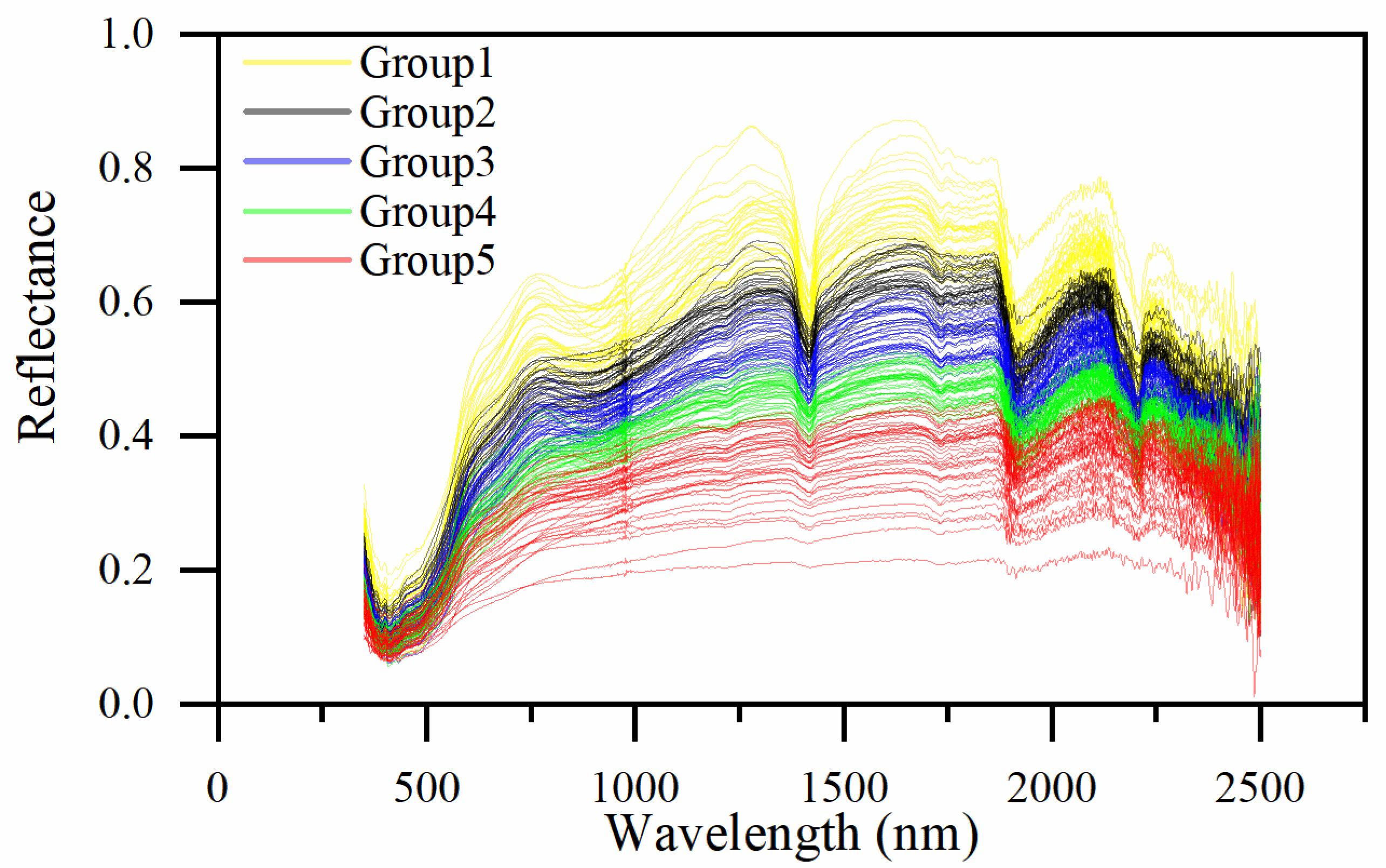
2.4.1. Spectral Similarity

Spectral similarity is determined by the spectrum curve shown in Figure 2. Figure 2 is commonly and popularly used to display soil spectra. In theory, as the composition levels in a soil sample increase, the spectral absorption will vary, potentially becoming weaker or stronger [52]. For example, a sample with high organic matter would absorb spectra strongly, resulting in low reflectance and placing the spectral curve at the bottom of the figure. Many researchers have observed this phenomenon [53]. To clearly show the spectral similarities, we use spectral curves to illustrate them and classify the samples. As shown in Figure 2, the spectra were classified into five groups based on spectral similarity. The classification is based on the reflectance values and their similarities to other spectra [54]. Group 1 has the highest reflectance, while Group 5 has the lowest. Reflectance gradually decreases from Group 1 to Group 5.

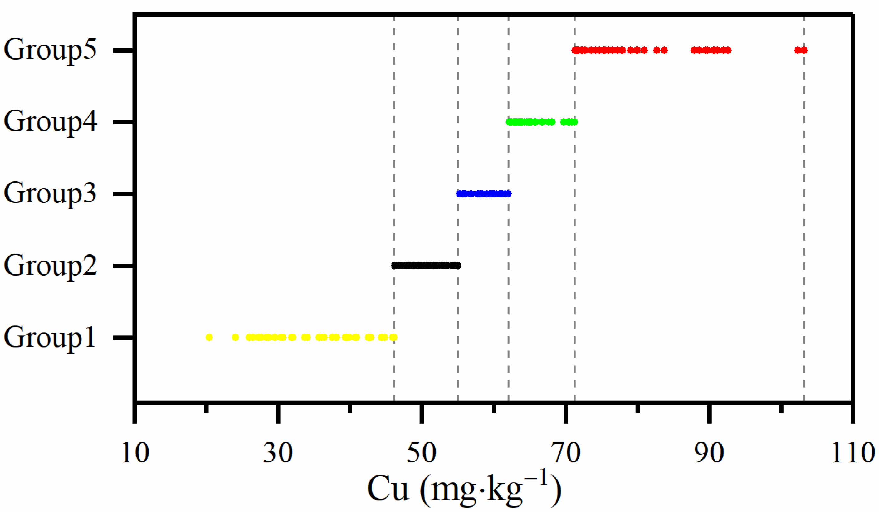
2.4.2. Compositional Similarity

Compositional similarity is determined by the Cu level, as shown in Figure 3. Compositional similarity is simply based on the absolute value of Cu levels. For example, a sample with 30 mg·kg⁻¹ is more similar to a sample with 31 mg·kg⁻¹ than to one with 50 mg·kg⁻¹. The samples were classified into five groups based on compositional similarity, as shown in Figure 3. Group 1 has the lowest Cu content, while Group 5 has the highest. The Cu content gradually increases from Group 1 to Group 5. The Cu content range for Groups 1 to 5 are 20.45–46.12 mg·kg⁻¹, 46.12–54.96 mg·kg⁻¹, 54.96–62.08 mg·kg⁻¹, 62.08–71.28 mg·kg⁻¹, and 71.28–103.24 mg·kg⁻¹, respectively.

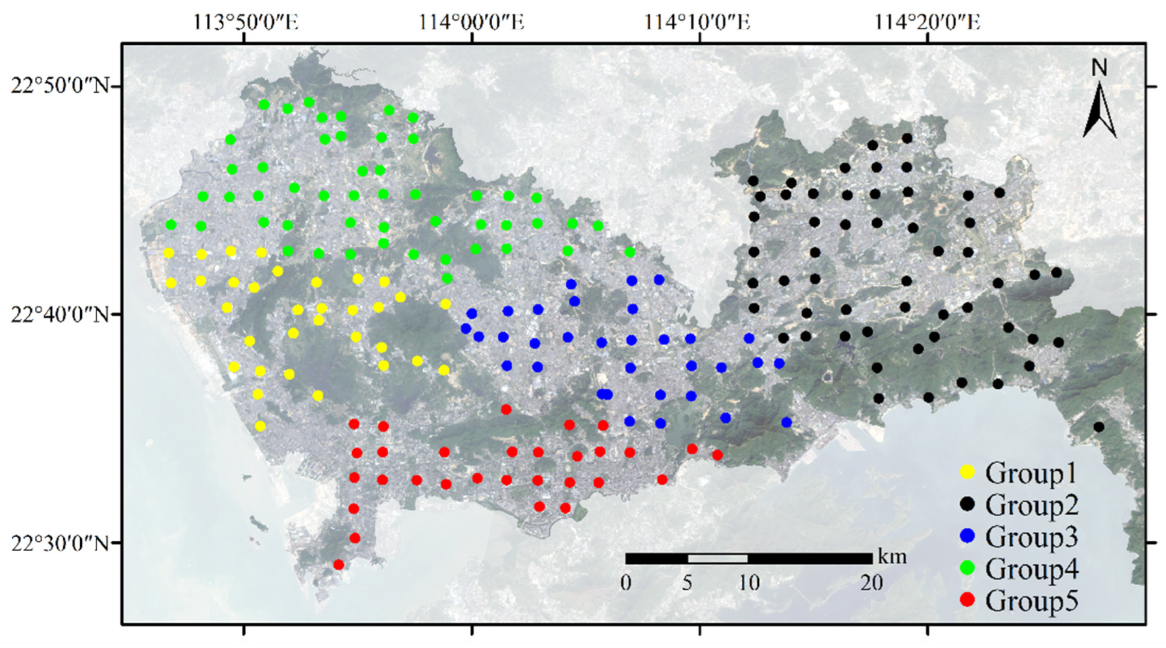
2.4.3. Spatial Similarity

Spatial similarity is determined by the spatial distance, as shown in Figure 4. The distance between samples clearly indicates spatial similarity. For example, a sample is more similar to one 10 m away than to one 100 m away. The samples were classified into five groups based on the spatial distance as shown in Figure 4. Each group contains samples that are geographically close to each other. In other words, the samples in each group are clustered together in terms of geographic distance. Each group covers a distinct area, clearly different from the areas covered by other groups.

2.5. Model Calibration

The calibration set comprises 80% of the samples, which is about 200 samples. The validation set consists of 20% of all samples, amounting to 50 samples. The 20%/80% split is a common ratio previously used by researchers [55,56]. The 20% of samples were chosen based on the order of Cu levels. For every five samples, one was selected for validation and the rest were used for the calibration set. The split ensures that the validation samples adequately represent the diversity of future samples. To compare the three similarities, the validation set consistently contains the same 50 samples, and the calibration set always includes the same 200 samples. The calibration set and validation set were then divided into five groups based on spectral, compositional, and spatial similarities, as described in Section 2.4 and shown in Figure 2, Figure 3 and Figure 4.

The calibration set was used to build Cu measurement models using Partial Least-Squares Regression (PLSR). PLSR is commonly used to build soil property measurement models [57]. It first projects the spectra into a low-dimensional space, where multiple regression is then performed. According to our previous work, mean centering (MC) is the most effective spectral pretreatment [13]. Leave-one-out cross-validation (LOOCV) was used to determine the number of latent variables (LVs). PLSR was carried out using the PLS_toolbox 8.1.1 (Eigenvector Research, Inc., Manson, WA, USA) in the MATLAB R2014a environment (The MathWorks, Inc., Natick, MA, USA).

2.6. Performance of Models

The validation set from Section 2.5 was used to test the performance of the Cu measurement model. The performance of the Cu measurement models was assessed using common indicators: residual predictive deviation (RPD), root mean square error of prediction (RMSEP), and the coefficient of determination in prediction ($R_p^2$).

3. Results

3.1. Descriptive of Statistics of Soil Samples

The soil Cu level in Shenzhen City ranged from 20.45 to 103.24 mg·kg⁻¹, with a mean value of 58.29 mg·kg⁻¹ (

Table 1. Sample divisions and descriptive statistics of soil Cu in spectral similarity. Group 1 has the highest reflectance, while Group 5 has the lowest. Reflectance gradually decreases from Group 1 to Group 5.

Spectral Similarity	Sample Set	Count	Cu (mg·kg−1)
			Range 1	Min	Max	Mean	Std 2	Skewness	Kurtosis	CV 3
Group 1	All	53	81.90	20.45	102.35	57.19	17.71	0.40	0.09	0.31
	Calibration	40	81.90	20.45	102.35	56.49	17.98	0.38	0.30	0.32
	Validation	13	57.01	33.83	90.84	59.35	17.37	0.58	−0.36	0.29
Group 2	All	49	68.57	24.05	92.62	57.50	15.88	0.32	−0.63	0.28
	Calibration	40	68.57	24.05	92.62	56.68	16.12	0.48	−0.36	0.28
	Validation	9	41.19	36.88	78.07	61.13	15.08	−0.49	−1.36	0.25
Group 3	All	50	70.55	26.51	97.06	56.09	15.10	0.05	0.63	0.27
	Calibration	40	63.22	26.51	89.73	55.15	15.00	−0.31	−0.02	0.27
	Validation	10	55.76	41.3	97.06	59.84	15.70	1.61	3.21	0.26
Group 4	All	50	55.71	28.08	83.79	55.91	13.96	−0.25	−0.43	0.25
	Calibration	40	55.13	28.66	83.79	56.59	13.33	−0.22	−0.32	0.24
	Validation	10	52.64	28.08	80.72	53.19	16.76	−0.16	−0.69	0.32
Group 5	All	48	78.03	25.21	103.24	65.07	13.39	0.17	1.90	0.21
	Calibration	40	62.46	40.78	103.24	66.51	12.93	0.68	0.88	0.19
	Validation	8	45.49	25.21	70.70	57.90	14.22	−2.06	5.05	0.25
Total	All	250	82.79	20.45	103.24	58.29	15.57	0.13	0.12	0.27
	Calibration	200	82.79	20.45	103.24	58.29	15.60	0.13	0.15	0.27
	Validation	50	71.85	25.21	97.06	58.30	15.63	0.13	0.12	0.27

¹ Range denotes the difference between the maximum and minimum observations. ² Std denotes the standard deviation. ³ CV denotes the coefficient of variation.

,

Table 2. Sample divisions and descriptive statistics of soil Cu in compositional similarity. Group 1 has the lowest Cu content, while Group 5 has the highest. The Cu content gradually increases from Group 1 to Group 5.

Compositional Similarity	Sample Set	Count	Cu (mg·kg−1)
			Range 1	Min	Max	Mean	Std 2	Skewness	Kurtosis	CV 3
Group 1	All	53	25.67	20.45	46.12	36.37	6.74	−0.46	−0.85	0.19
	Calibration	40	25.67	20.45	46.12	36.35	6.81	−0.48	−0.77	0.19
	Validation	10	19.66	25.21	44.87	36.42	6.78	−0.43	−1.11	0.19
Group 2	All	50	8.7	46.26	54.96	50.72	2.46	0.1	−1.01	0.05
	Calibration	40	8.7	46.26	54.96	50.71	2.47	0.1	−0.99	0.05
	Validation	10	7.91	47.01	54.92	50.74	2.57	0.13	−0.93	0.05
Group 3	All	50	6.85	55.23	62.08	58.77	2.06	−0.32	−1.15	0.04
	Calibration	40	6.85	55.23	62.08	58.78	2.06	−0.3	−1.15	0.04
	Validation	10	6.46	55.52	61.98	58.81	2.17	−0.28	−1.06	0.04
Group 4	All	50	9.06	62.22	71.28	65.2	2.7	1.09	0.05	0.04
	Calibration	40	9.06	62.22	71.28	65.2	2.68	1.07	−0.02	0.04
	Validation	10	8.37	62.33	70.7	65.19	2.78	1.2	0.49	0.04
Group 5	All	50	31.93	71.31	103.24	80.39	8.64	1.03	0.32	0.11
	Calibration	40	31.93	71.31	103.24	80.38	8.57	0.98	0.1	0.11
	Validation	10	25.59	71.47	97.06	80.35	8.76	0.93	−0.34	0.11
Total	All	250	82.79	20.45	103.24	58.29	15.57	0.13	0.12	0.27
	Calibration	200	82.79	20.45	103.24	58.29	15.60	0.13	0.15	0.27
	Validation	50	71.85	25.21	97.06	58.30	15.63	0.13	0.12	0.27

¹ Range denotes the difference between the maximum and minimum observations. ² Std denotes the standard deviation. ³ CV denotes the coefficient of variation.

and

Table 3. Sample divisions and descriptive statistics of soil Cu in spatial similarity. Each group contains samples that are geographically close to each other. Each group covers a distinct area, clearly different from the areas covered by other groups.

Spatial Similarity	Sample Set	Count	Cu (mg·kg−1)
			Range 1	Min	Max	Mean	Std 2	Skewness	Kurtosis	CV 3
Group 1	All	43	61.87	40.48	102.35	64.51	13.69	0.5	0.43	0.21
	Calibration	33	61.51	40.84	102.35	64.32	13.59	0.75	0.8	0.21
	Validation	10	50.36	40.48	90.84	65.15	14.77	−0.24	0.37	0.23
Group 2	All	69	76.61	20.45	97.06	53.72	16.24	0.17	0.22	0.3
	Calibration	54	70.39	20.45	90.84	53.37	16.28	0.07	−0.2	0.31
	Validation	15	71.85	25.21	97.06	54.96	16.61	0.56	2.7	0.3
Group 3	All	40	49.52	29.54	79.06	54.84	13.6	−0.08	−1.07	0.25
	Calibration	33	49.52	29.54	79.06	55.41	13.73	−0.14	−0.95	0.25
	Validation	7	34.59	36.88	71.47	52.18	13.67	0.24	−1.81	0.26
Group 4	All	61	79.19	24.05	103.24	59.56	15.94	0.27	0.53	0.27
	Calibration	50	79.19	24.05	103.24	60.42	15.72	0.28	0.85	0.26
	Validation	11	57.58	30.5	88.08	55.61	17.08	0.37	−0.04	0.31
Group 5	All	37	58.26	33.73	91.99	61.22	15.02	0.1	−0.55	0.25
	Calibration	30	58.26	33.73	91.99	60.1	15.76	0.21	−0.59	0.26
	Validation	7	25.8	54.92	80.72	66.03	10.91	0.44	−2.19	0.17
Total	All	250	82.79	20.45	103.24	58.29	15.57	0.13	0.12	0.27
	Calibration	200	82.79	20.45	103.24	58.29	15.60	0.13	0.15	0.27
	Validation	50	71.85	25.21	97.06	58.30	15.63	0.13	0.12	0.27

¹ Range denotes the difference between the maximum and minimum observations. ² Std denotes the standard deviation. ³ CV denotes the coefficient of variation.

). The mean value of 58.29 mg·kg⁻¹ was higher than the background level of 22 mg·kg⁻¹ [58]. The likely reason is that this city has been impacted by rapid industrialization. The coefficient of variation (CV) was 0.27, indicating a medium level of variability (0.1 < CV < 1.0). The skewness was 0.13 and the kurtosis was 0.12, both close to zero, indicating a normal distribution. Overall, the statistics of the calibration and validation sets are similar.

For spectral similarity, the mean values for groups 1 through 5 were 57.19, 57.50, 56.09, 55.91, and 65.07 mg·kg⁻¹, respectively (Table 1). The mean values of the five groups showed a slight difference. For spatial similarity, the mean values followed a similar pattern to those of spectral similarity (Table 3). But for compositional similarity, the mean values were 36.37, 50.72, 58.77, 65.2, and 80.39 mg·kg⁻¹, showing a clear increase from low to high (Table 2). This is because the division is based on Cu values arranged in ascending order (Figure 2). Thus, in terms of Cu levels, divisions based on spectral and spatial similarities slightly changed the groups, while divisions based on compositional similarity made the groups more distinct from each other.

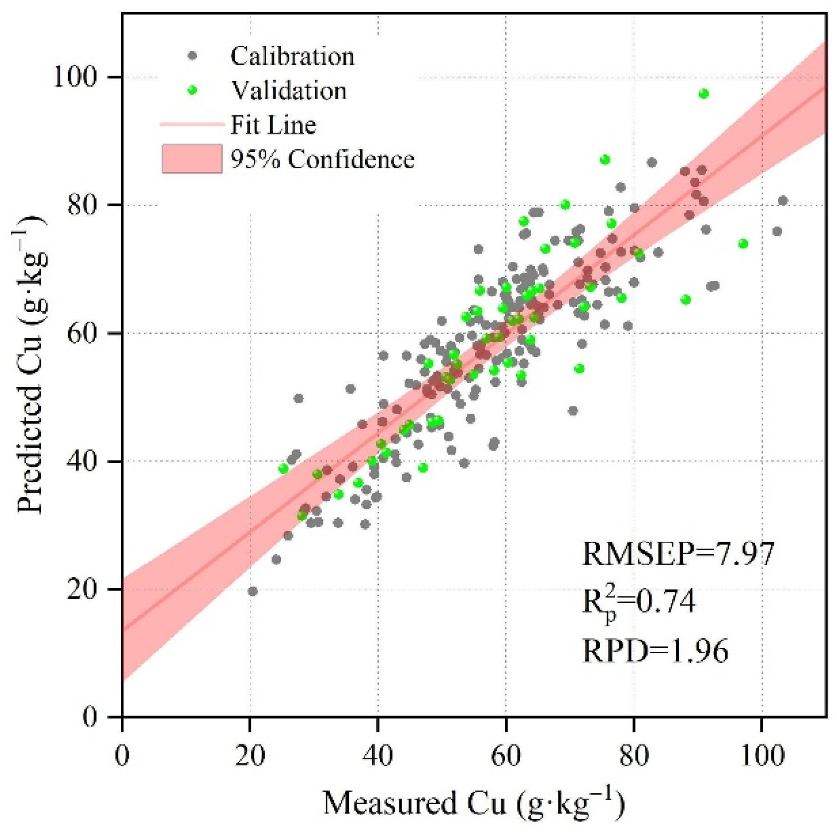
3.2. Measurement Accuracy of Cu Models without Considering Similarity

When similarity was not considered, the Cu measurement model produced an acceptable result (Figure 5). The RMSEP is 7.97 mg·kg⁻¹, the $R_p^2$ is 0.74, and RPD is 1.96. Most samples are closely aligned with the fit line. The three indicators suggest that it is feasible to measure Cu levels in soil within a large city using vis-NIR spectroscopy with satisfactory accuracy. However, some samples are far from the Fit Line, indicating significant errors. These errors may result from complex spectra, the wide range of Cu content, and the large spatial area. Therefore, considering spectral, compositional, and spatial similarities has the potential to reduce soil diversity and improve the Cu estimation model.

3.3. Measurement Accuracy of Cu Models when Considering Similarity

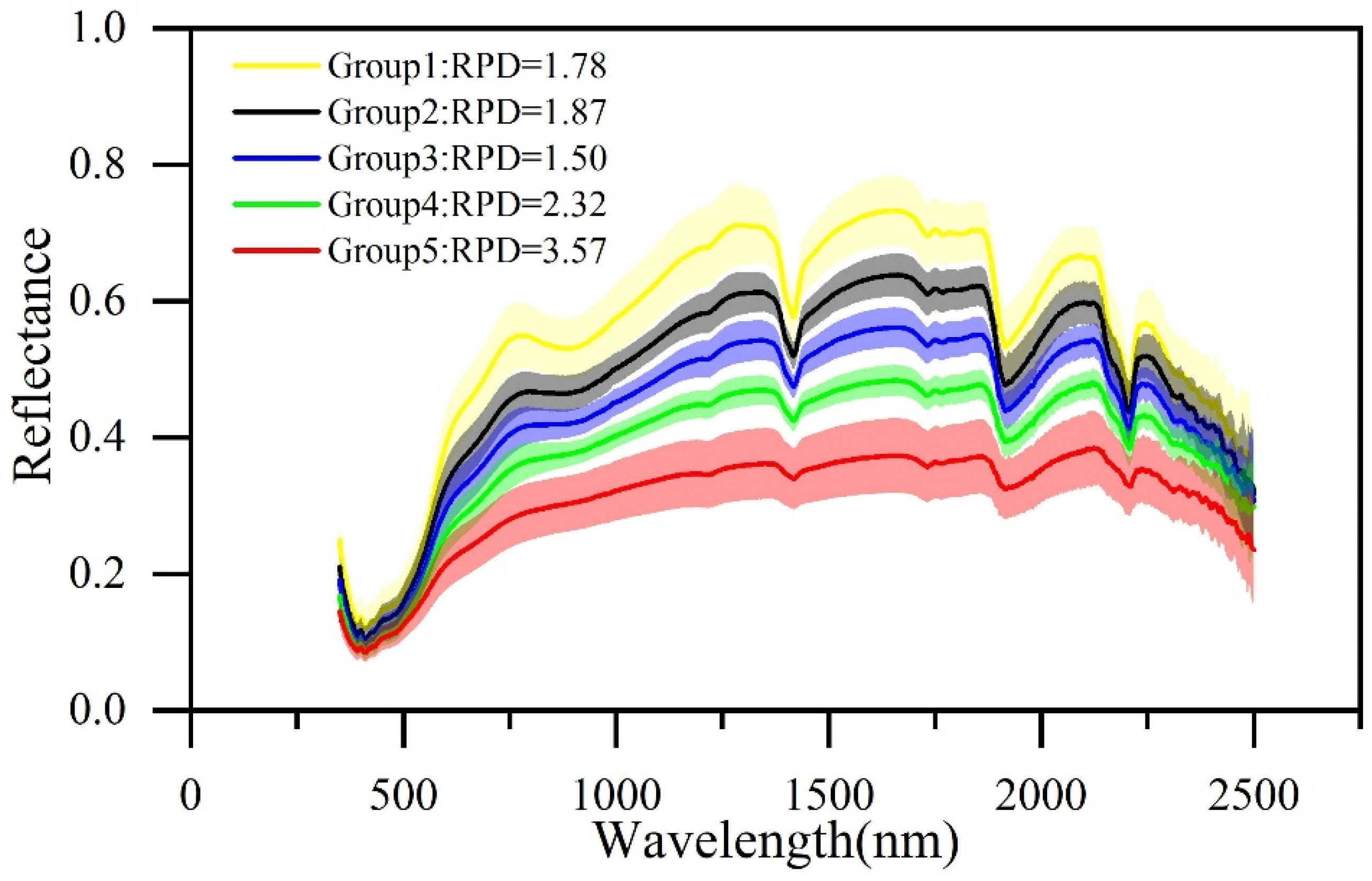
3.3.1. Spectral Similarity

In this section, spectral similarity was used to divide the samples into five groups, and a separate Cu measurement model was built for each group. The performance of the Cu measurement model is displayed in

Table 4. Summary statistics for the soil Cu measurement model with consideration of spectral similarity.

Spectral Similarity		Calibration			Validation					LVs
		N	${\mathit{R}}_{\mathit{c}\mathit{v}}^2$	${\mathbf{R}\mathbf{M}\mathbf{S}\mathbf{E}}_{\mathit{c}\mathit{v}}$	n	Std	${\mathit{R}}_{\mathit{p}}^2$	RMSEP	RPD
No Group	Not Croup	200	0.67	8.90	50	15.63	0.74	7.97	1.96	6
Group	Group 1	40	0.56	12.05	13	17.37	0.70	9.78	1.78	5
	Group 2	40	0.53	11.07	9	15.08	0.90	8.05	1.87	4
	Group 3	40	0.48	10.76	10	15.70	0.54	10.47	1.50	4
	Group 4	40	0.47	9.85	10	16.76	0.82	7.22	2.32	4
	Group 5	40	0.10	13.04	8	14.22	0.99	3.98	3.57	5
	Overall	200	0.48	11.41	50	15.63	0.71	8.45	1.85	-

$R_{cv}^2$ denotes the coefficient of determination in cross-validation. ${\mathrm{R}\mathrm{M}\mathrm{S}\mathrm{E}}_{cv}$ denotes the root mean square error in cross-validation. Std denotes the standard deviation. RMSEP denotes the root mean square error of prediction. $R_p^2$ denotes the coefficient of determination in prediction. RPD denotes the residual predictive deviation. LVs denotes latent variables.

and Figure 6.

For the five groups, the performance of the Cu measurement model varied (Table 4 and Figure 6). Group 5 had the best performance, with an $R_p^2$ of 0.99 and an RPD of 3.57. Group 4 achieved satisfactory results with an $R_p^2$ of 0.82 and an RPD of 2.32. Groups 4 and 5 performed better than the model that did not consider spectral similarity. However, Group 3 obtained the worst results, with an $R_p^2$ of 0.54 and an RPD of 1.50. Groups 1 and 2 achieved similar results to the model that did not consider spectral similarity, with RPD values of 1.78 and 1.87, respectively.

Overall, the Cu measurement model that considered spectral similarity performed slightly worse than the one that did not (Table 4 and Figure 6). Considering the fact that spectral similarity slightly decreased the $R_p^2$ from 0.74 to 0.71 and the RPD from 1.96 to 1.85. As shown in Figure 6, the spectrum was divided into clearly different groups, but no improvement was observed. Spectral similarity improved the performance for low reflectance spectra, such as Groups 4 and 5, but did not work well for high reflectance spectra, like Groups 1 and 2.

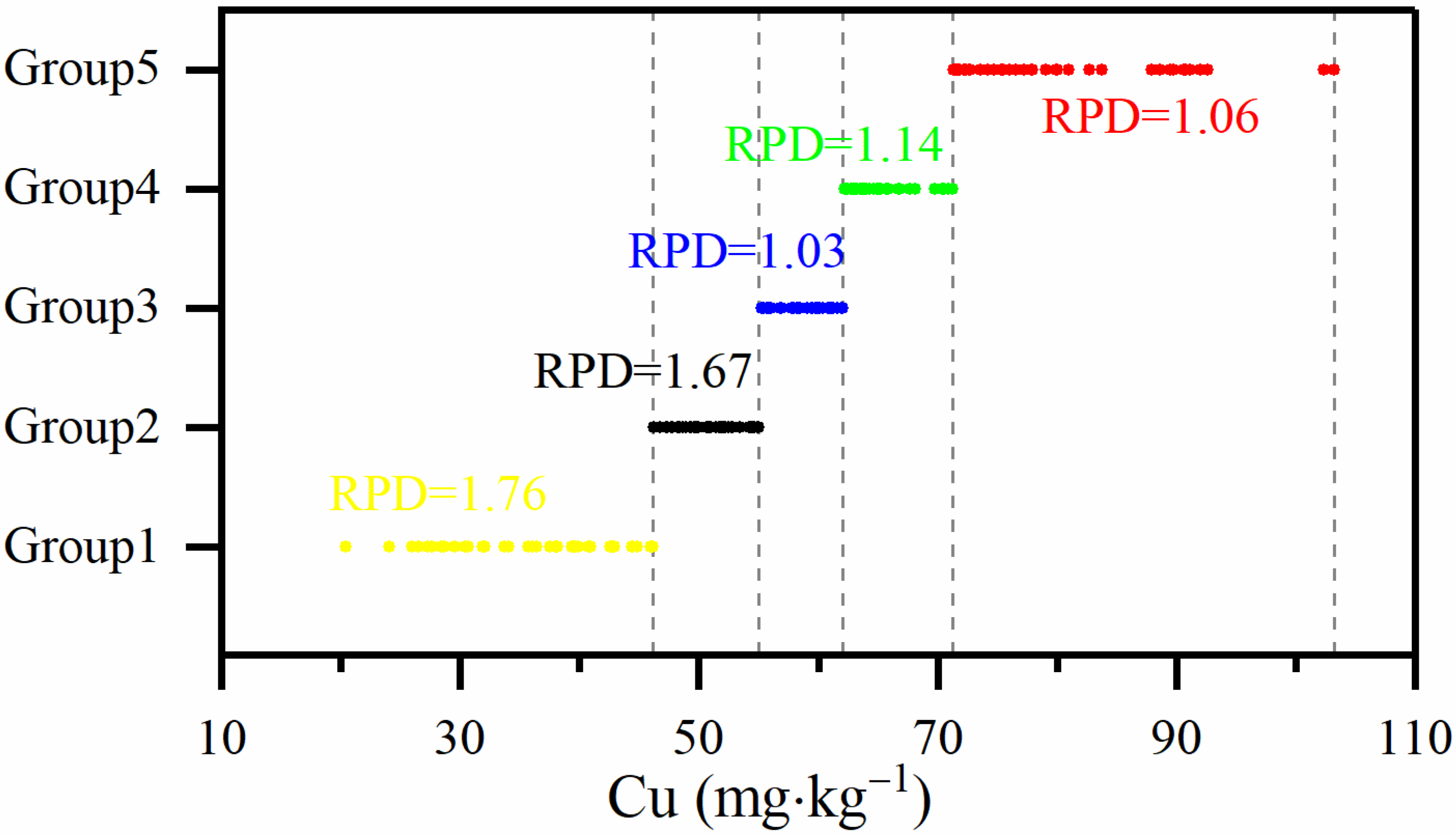
3.3.2. Compositional Similarity

In this section, compositional similarity was used to divide the samples into five groups, and a separate Cu measurement model was built for each group. The performance of the Cu measurement model is displayed in

Table 5. Summary statistics for the soil Cu measurement model with consideration of compositional similarity.

Compositional Similarity		Calibration			Validation					LVs
		n	${\mathit{R}}_{\mathit{c}\mathit{v}}^2$	${\mathbf{R}\mathbf{M}\mathbf{S}\mathbf{E}}_{\mathit{c}\mathit{v}}$	n	Std	${\mathit{R}}_{\mathit{p}}^2$	RMSEP	RPD
No Group	Not Croup	200	0.67	8.90	50	15.63	0.74	7.97	1.96	6
Group	Group 1	40	0.20	6.55	10	6.78	0.67	3.85	1.76	5
	Group 2	40	0.09	3.79	10	2.57	0.61	1.54	1.67	5
	Group 3	40	0.07	2.12	10	2.17	0.04	2.03	1.07	1
	Group 4	40	0.03	3.02	10	2.78	0.15	2.43	1.14	3
	Group 5	40	0.08	8.93	10	8.76	0.01	8.30	1.06	1
	Overall	200	0.88	5.49	50	15.63	0.92	4.38	3.57	-

$R_{cv}^2$ denotes the coefficient of determination in cross-validation. ${\mathrm{R}\mathrm{M}\mathrm{S}\mathrm{E}}_{cv}$ denotes the root mean square error in cross-validation. Std denotes the standard deviation. RMSEP denotes the root mean square error of prediction. $R_p^2$ denotes the coefficient of determination in prediction. RPD denotes the residual predictive deviation. LVs denotes latent variables.

and Figure 7.

For the five groups, the Cu measurement model’s performance varied, with $R_p^2$ ranging from 0.04 to 0.67 and RPD ranging from 1.06 to 1.76 (Table 5 and Figure 7). Group 1 performed best with an $R_p^2$ of 0.67 and an RPD of 1.76. Group 2 obtained similar results to Group 1, with an $R_p^2$ of 0.61 and an RPD of 1.67. Groups 3, 4 and 5 performed poorly, with $R_p^2$ of 0.01–0.15 and RPD of 1.06–1.14. Compared to the model that did not consider compositional similarity, Groups 1–5 performed worse, particularly Groups 3, 4, and 5.

Overall, considering compositional similarity significantly improved the Cu measurement model. The $R_p^2$ increased from 0.74 to 0.92, and the RPD increased from 1.96 to 3.57. As shown in Figure 7, considering compositional similarity worked poorly for high Cu levels (Groups 3–5) but was more effective for low Cu levels (Groups 1 and 2).

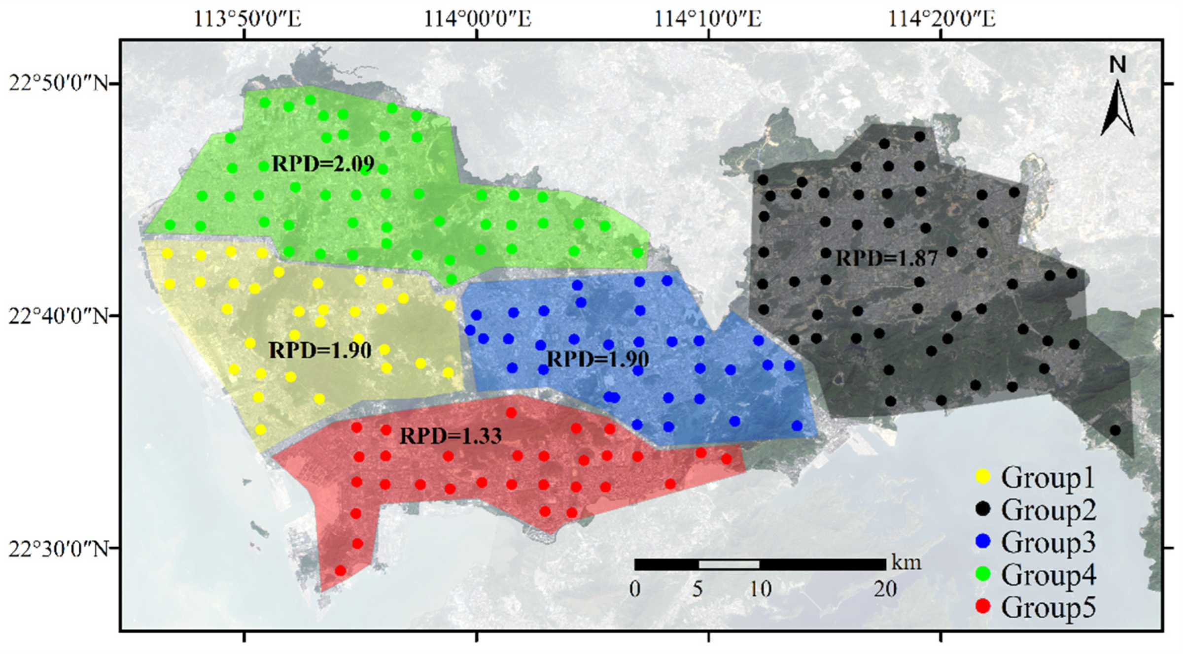
3.3.3. Spatial Similarity

In this section, spatial similarity was used to divide the samples into five groups, and a separate Cu measurement model was built for each group. The performance of the Cu measurement model is displayed in

Table 6. Performance of the soil Cu measurement model when considering spatial similarity.

Spatial Similarity		Calibration			Validation					LVs
		n	${\mathit{R}}_{\mathit{c}\mathit{v}}^2$	${\mathbf{R}\mathbf{M}\mathbf{S}\mathbf{E}}_{\mathit{c}\mathit{v}}$	n	Std	${\mathit{R}}_{\mathit{p}}^2$	RMSEP	RPD
No Group	Not Croup	200	0.67	8.90	50	15.63	0.74	7.97	1.96	6
Group	Group 1	33	0.61	8.44	10	14.77	0.81	7.78	1.90	6
	Group 2	54	0.51	11.76	15	16.61	0.72	8.88	1.87	7
	Group 3	33	0.22	12.53	7	13.67	0.79	8.04	1.70	3
	Group 4	50	0.58	10.28	11	17.08	0.77	8.16	2.09	6
	Group 5	30	0.37	12.32	7	10.91	0.41	8.19	1.33	2
	Overall	200	0.51	11.14	50	15.63	0.73	8.30	1.88	-

$R_{cv}^2$ denotes the coefficient of determination in cross-validation. ${\mathrm{R}\mathrm{M}\mathrm{S}\mathrm{E}}_{cv}$ denotes the root mean square error in cross-validation. Std denotes the standard deviation. RMSEP denotes the root mean square error of prediction. $R_p^2$ denotes the coefficient of determination in prediction. RPD denotes the residual predictive deviation. LVs denotes latent variables.

and Figure 8.

For the five groups, the Cu measurement model generally performed well (Table 6 and Figure 8). Group 4 performed best with an $R_p^2$ of 0.77 and an RPD of 2.09. Groups 1, 2, and 3 also achieved good results, with an $R_p^2$ of 0.72–0.81 and an RPD of 1.70–1.90. Group 5 had the worst result, with an $R_p^2$ of 0.41 and an RPD of 1.33. Compared to the model that did not consider spatial similarity, Group 4 performed better, Groups 1–3 performed similarly, and Group 5 performed worse.

Overall, considering spatial similarity did not significantly change the Cu measurement model. The $R_p^2$ decreased slightly from 0.74 to 0.73, and the RPD also decreased slightly from 1.96 to 1.88. As shown in Figure 8, the samples were divided into distinct spatial groups, but this did not lead to any improvement. Group 5 is the central area of the city, accounting for 50% of the city’s GDP. It is also the most densely populated area with 18,000 people per square kilometer. Thus, considering spatial similarity was less effective in highly developed areas (Group 5) but worked better in less developed areas (Group 4).

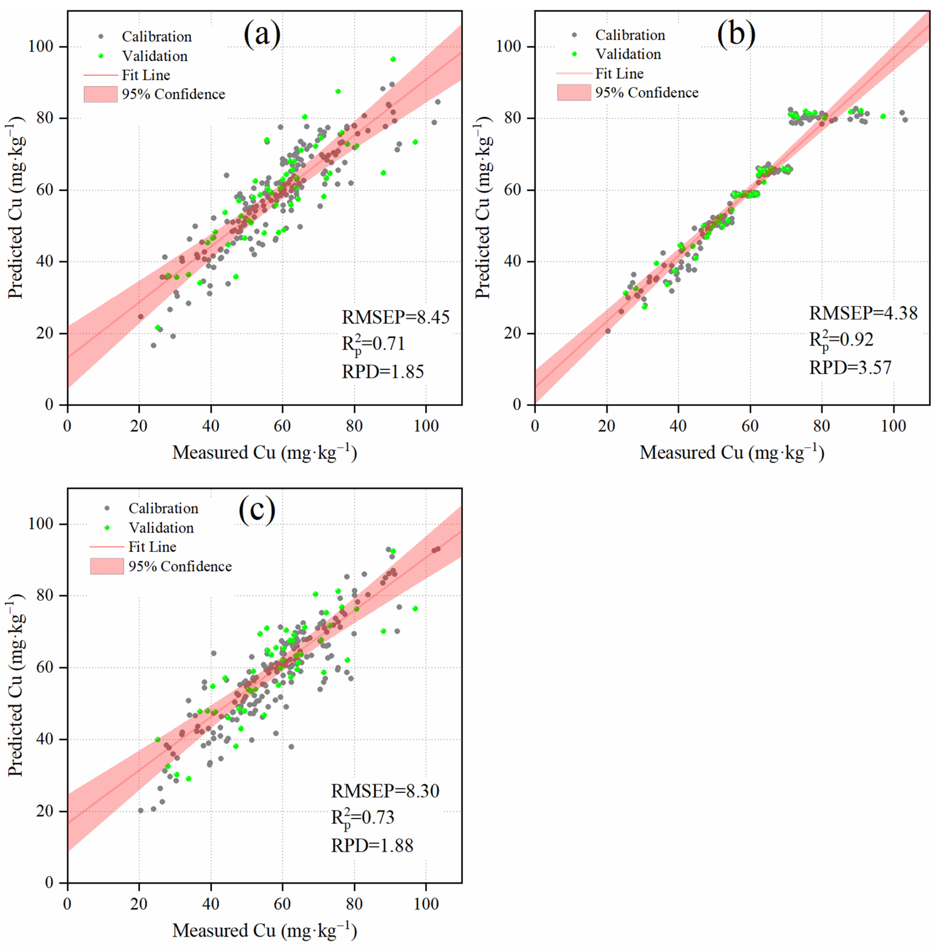
3.3.4. Comparing Spectral, Compositional, and Spatial Similarities

The performance order of the Cu measurement model is compositional similarity > spatial similarity > spectral similarity (Figure 9). Compositional similarity performed the best, with an $R_p^2$ of 0.92 and an RPD of 3.57. The result is highly satisfactory. As shown in Figure 9b, most samples were closely aligned with the fit line and fell within the 95% confidence area. However, for both spectral and spatial similarities, the performance was considerably lower. Spatial similarity achieved an $R_p^2$ of 0.73 and an RPD of 1.88 (Figure 9c), while compositional similarity obtained an $R_p^2$ of 0.71 and an RPD of 1.85 (Figure 9a). The difference in $R_p^2$ between 0.92 and 0.73 and the difference in RPD between 3.57 and 1.88 were significant. Thus, compositional similarity significantly performed better than spatial and spectral similarities. Moreover, spatial similarity performed slightly better than spectral similarity.

Compared to the model that did not consider similarity, considering compositional similarity significantly improved the model (Figure 5 and Figure 9). Considering compositional similarity increased the $R_p^2$ from 0.74 to 0.92 and the RPD from 1.96 to 3.57 while decreasing the RMSEP from 7.97 to 4.38 mg·kg⁻¹. For spectral and spatial similarities, the change was not obvious. Considering spectral similarity led to a slight decrease in $R_p^2$ from 0.74 to 0.71. Similarly, considering spatial similarity also slightly reduced the $R_p^2$ from 0.74 to 0.73. Thus, among the three similarities, considering compositional similarity is the most successful with great improvement. Therefore, among the three types of similarities, compositional similarity contributes the most to successful improvement.

Focusing on one type of similarity makes it difficult to ensure similarity in the other two types (Figure 10). For instance, when focusing on spectral similarity, samples in each group clustered closely in spectral space (Figure 10a). However, in compositional (Figure 10a) and spatial spaces (Figure 10b), the samples in each group were spread out, with no clear boundaries for each group. This phenomenon also occurred when focusing on compositional similarities (Figure 10d–f) and spatial similarities (Figure 10g–i). Thus, ensuring all three types of similarities simultaneously is challenging, and prioritizing one type of similarity often requires sacrificing the other two types.

4. Discussion

4.1. Performance of Estimating Cu in a Megacity by Vis-NIR Spectroscopy

In this study, vis-NIR spectroscopy was successfully used to measure soil Cu levels in a large city with acceptable accuracy. The best model achieved an $R_p^2$ of 0.92 and an RPD of 3.57 (Table 5). Some studies have reported similar findings; for example, Gozukara et al. (2022) achieved an $R_p^2$ of 0.90 and an RPD of 2.66 [59]. Pyo et al. (2020) obtained an $R_p^2$ of 0.74 [60]. However, other researchers have obtained much worse results, with $R_p^2$ of 0.53 [61], 0.26 [62], and 0.01 [63]. The variations in performance could be due to differences in sample size, sampling location, soil type, and environmental conditions. In comparison, our study achieved a much more acceptable result for estimating Cu using vis-NIR spectroscopy. While our method primarily focuses on heavy metal Cu estimation, it may also be applicable to other heavy metals, such as chromium (Cr), and other soil properties like soil organic matter (SOM). Further research is needed to explore these possibilities.

The important wavelengths were identified using the variable importance in projection (VIP) method (Figure 11). Wavelengths with VIP values greater than 1 were considered highly correlated and significant for estimating soil Cu [64]. In this study, the important wavelengths identified were 350–568 nm, 747–789 nm, 1356–1401 nm, 1940–1962 nm, 1979–1988 nm, 2409–2419 nm, 2434–2438 nm, and 2470–2500 nm. Numerous other researchers have also highlighted the importance of wavelengths at 350–568 nm, 747–789 nm, 1356–1401 nm, 1940–1962 nm, and 2409–2419 nm [62,65,66,67]. However, fewer researchers have reported the importance of wavelengths at 1979–1988 nm, 2434–2438 nm, and 2470–2500 nm.

4.2. Spectral Similarity vs. Compositional Similarity vs. Spatial Similarity

Spectral similarity slightly degraded the Cu measurement model (Figure 6). Considering spectral similarity slightly decreased the $R_p^2$ from 0.74 to 0.71 and the RPD from 1.96 to 1.85. Our results differed significantly from previous studies where improvements were observed. Shi et al. (2015) utilized spectral similarity, resulting in an increase in the $R_p^2$ value from 0.50 to 0.69 and an improvement in RPD from 1.41 to 1.77 [14]. Qi et al. (2021) also employed spectral similarity, leading to an enhancement in RPD from 1.87 to 2.12 [22]. In a more recent study, Liu et al. (2024) utilized spectral similarity for sample selection, resulting in an $R_p^2$ increase of more than 15% [24]. The reason behind this could be due to two factors: (i) the study area: our study area is a megacity with 17.79 million people and a GDP of 482 billion dollars. The soil here is heavily influenced by human activities, making it very different from farmland and complicating the spectral curves. (ii) Heavy metals: soil Cu shows little to no spectral response in the vis-NIR regions [19]. Its spectral characteristics are mainly tied to its association with other properties like soil SOM, which has a more active spectral response [29]. Thus, soil Cu’s spectral characteristics are less distinct compared to properties like SOM, commonly studied in previous research. In addition, it was observed that spectral similarity yielded better results when dealing with low-reflectance spectra, while its effectiveness was limited when dealing with high-reflectance spectra (Figure 6).

Compositional similarity significantly improved the Cu measurement model (Figure 7). The $R_p^2$ increased from 0.74 to 0.92, and the RPD increased from 1.96 to 3.57. According to this study, many other studies have also reported improvements when considering compositional similarity. Madari et al. (2005) used the similarity of soil textural properties to achieve more accurate results [40]. Jaconi et al. (2017) considered the similarity of soil properties (depth, pH, and soil texture) and obtained better results [39]. Hong et al. (2017) found that considering the similarity of soil moisture could improve model performance [33]. However, some researchers have found that compositional similarity did not always work. For instance, Qi et al. (2021) used compositional similarity, but their predictions were unsuccessful [22]. In general, taking into account compositional similarity tends to enhance model accuracy. This is likely because samples with similar compositions exhibit a comparable relationship between spectra and soil composition. Consequently, a cluster of similar samples can lead to a more effective model. Additionally, considering compositional similarity was less effective for high Cu levels but more effective for low Cu levels (Figure 7).

Spatial similarity did not significantly impact the Cu measurement model (Figure 8). The $R_p^2$ value decreased slightly from 0.74 to 0.73, and the RPD decreased slightly from 1.96 to 1.88. Our results differed from many previous studies. Peng et al. (2013) found that using the spatially closest samples achieved the highest RPD of 3.7 [34]. Nocita et al. (2014) included spatial information in the distance computation between samples and provided the most accurate soil organic carbon (SOC) predictions [38]. Shi et al. (2015) reported that using spatial similarity increased the $R_p^2$ value from 0.69 to 0.74 and the RPD from 1.77 to 1.96 [14]. Tziolas et al. (2019) also considered spatial similarity and obtained better results [27]. As shown in Figure 8, dividing the samples into distinct spatial groups did not lead to any improvement in the model’s performance. The reason for this might be similar to the spectral similarity discussed above in two aspects: the study area and heavy metals. Our study area is in a large city where human activities heavily influence the soil, making it very different from natural soils like those found in farmland. Most previous studies focused on either soil organic carbon or soil organic matter, which are derived from either natural sources or fertilizers. However, soil Cu mainly comes from industrial sources and factories, making it more complex and challenging to predict using spatial similarity. In addition, In addition, we found that taking spatial similarity into account was not as effective in highly developed regions but yielded better results in less developed areas.

The performance ranking of the Cu measurement model was: compositional similarity > spatial similarity > spectral similarity (Figure 9). Most studies focused on one type of similarity [35,41,52]. Our study successfully compared three types of similarity and identified which one was most important. The $R_p^2$ values for compositional, spatial, and spectral similarities were 0.92, 0.73, and 0.71, respectively. Correspondingly, the RPD values for these similarities were 3.57, 1.88, and 1.85. Compositional similarity was the best and significantly outperformed the other two types of similarity. In simpler terms, if samples have similar Cu concentrations, their vis-NIR model is likely to be similar. However, if samples have similar spectra or geography, it does not guarantee that their vis-NIR model will be similar. The reason is that compositional clusters are less influenced by external factors, such as human activities, compared to spectral or spatial clusters. Urban soils are heavily affected by human activities, making it difficult for spectral and spatial clusters to ensure consistency in Cu estimation models. However, compositional clusters are less affected, leading to more consistent Cu estimation models.

Ensuring all three types of similarities simultaneously is challenging, and prioritizing one type of similarity often requires sacrificing the other two types (Figure 10). Some researchers have also obtained similar results. Ramirez-Lopez et al. (2013) found that samples using spectral similarity showed a low degree of compositional similarity [28]. The reason behind this is that soil Cu could be influenced by human activities, especially in big cities. A small spatial area might contain diverse concentrations of Cu and different spectral curves. Thus, it is challenging to maintain high levels of similarity across all three aspects simultaneously.

5. Conclusions

The present study compared spectral, compositional, and spatial similarities in estimating Cu levels in a large city using vis-NIR spectroscopy. Vis-NIR spectroscopy is cheaper, faster, and more environmentally friendly than traditional methods like the diethylenetriamine penta-acetic acid (DTPA) method. From our results, we draw the following conclusions: (i) the performance ranking of the Cu measurement model was: compositional similarity > spatial similarity > spectral similarity. Compositional similarity performed significantly better than spatial and spectral similarities. Spatial similarity performed slightly better than spectral similarity. (ii) Ensuring all three types of similarities simultaneously is challenging, and prioritizing one type of similarity often requires sacrificing the other two types.

Although we successfully compared spectral, compositional, and spatial similarities in estimating Cu levels, further research on soil Cu measurement is still needed. While our study focused on heavy metal Cu in a large urban area, our approach could also be applied to smaller areas, farmland, and other soil properties like Cr and SOM.

References

1. Wang, S.; Cai, L.-M.; Wen, H.-H.; Luo, J.; Wang, Q.-S.; Liu, X. Spatial distribution and source apportionment of heavy metals in soil from a typical county-level city of Guangdong Province, China. Sci. Total Environ. 2019, 655, 92–101. [Google Scholar] [CrossRef]
2. Liu, L.L.; Liu, Q.Y.; Ma, J.; Wu, H.W.; Qu, Y.J.; Gong, Y.W.; Yang, S.H.; An, Y.F.; Zhou, Y.Z. Heavy metal(loid)s in the topsoil of urban parks in Beijing, China: Concentrations, potential sources, and risk assessment. Environ. Pollut. 2020, 260, 114083. [Google Scholar] [CrossRef]
3. Hou, D.; O’Connor, D.; Igalavithana, A.D.; Alessi, D.S.; Luo, J.; Tsang, D.C.; Sparks, D.L.; Yamauchi, Y.; Rinklebe, J.; Ok, Y.S. Metal contamination and bioremediation of agricultural soils for food safety and sustainability. Nat. Rev. Earth Environ. 2020, 1, 366–381. [Google Scholar] [CrossRef]
4. Xu, D.Y.; Chen, S.C.; Xu, H.Y.; Wang, N.; Zhou, Y.; Shi, Z. Data fusion for the measurement of potentially toxic elements in soil using portable spectrometers. Environ. Pollut. 2020, 263, 114649. [Google Scholar] [CrossRef] [PubMed]
5. Zhang, X.; Yan, L.; Liu, J.; Zhang, Z.; Tan, C. Removal of Different Kinds of Heavy Metals by Novel PPG-nZVI Beads and Their Application in Simulated Stormwater Infiltration Facility. Appl. Sci. 2019, 9, 4213. [Google Scholar] [CrossRef]
6. Alengebawy, A.; Abdelkhalek, S.T.; Qureshi, S.R.; Wang, M.-Q. Heavy metals and pesticides toxicity in agricultural soil and plants: Ecological risks and human health implications. Toxics 2021, 9, 42. [Google Scholar] [CrossRef] [PubMed]
7. Xu, J.K.; Yang, L.X.; Wang, Z.Q.; Dong, G.C.; Huang, H.Y.; Wang, Y.L. Toxicity of copper on rice growth and accumulation of copper in rice grain in copper contaminated soil. Chemosphere 2006, 62, 602–607. [Google Scholar] [CrossRef]
8. Sun, G.L.; Reynolds, E.E.; Belcher, A.M. Designing yeast as plant-like hyperaccumulators for heavy metals. Nat. Commun. 2019, 10, 5080. [Google Scholar] [CrossRef] [PubMed]
9. Li, X.; Pan, W.; Li, D.; Gao, W.; Zeng, R.; Zheng, G.; Cai, K.; Zeng, Y.; Jiang, C. Can fusion of vis-NIR and MIR spectra at three levels improve the prediction accuracy of soil nutrients? Geoderma 2024, 441, 116754. [Google Scholar] [CrossRef]
10. Krzebietke, S.; Daszykowski, M.; Czarnik-Matusewicz, H.; Stanimirova, I.; Pieszczek, L.; Sienkiewicz, S.; Wierzbowska, J. Monitoring the concentrations of Cd, Cu, Pb, Ni, Cr, Zn, Mn and Fe in cultivated Haplic Luvisol soils using near-infrared reflectance spectroscopy and chemometrics. Talanta 2023, 251, 123749. [Google Scholar] [CrossRef]
11. Wang, C.; Yang, Z.; Yuan, X.; Browne, P.; Chen, L.; Ji, J. The influences of soil properties on Cu and Zn availability in soil and their transfer to wheat t (Triticum aestivum L.) in the Yangtze River delta region, China. Geoderma 2013, 193, 131–139. [Google Scholar] [CrossRef]
12. Guo, B.; Zhang, B.; Su, Y.; Zhang, D.; Wang, Y.; Bian, Y.; Suo, L.; Guo, X.; Bai, H. Retrieving zinc concentrations in topsoil with reflectance spectroscopy at Opencast Coal Mine sites. Sci. Rep. 2021, 11, 19909. [Google Scholar] [CrossRef] [PubMed]
13. Liu, Y.; Shi, T.; Lan, Z.; Guo, K.; Zhuang, D.; Zhang, X.; Liang, X.; Qiu, T.; Zhang, S.; Chen, Y. Estimating the Soil Copper Content of Urban Land in a Megacity Using Piecewise Spectral Pretreatment. Land 2024, 13, 517. [Google Scholar] [CrossRef]
14. Shi, Z.; Ji, W.; Viscarra Rossel, R.A.; Chen, S.; Zhou, Y. Prediction of soil organic matter using a spatially constrained local partial least squares regression and the Chinese vis–NIR spectral library. Eur. J. Soil Sci. 2015, 66, 679–687. [Google Scholar] [CrossRef]
15. Liu, Y.; Liu, Y.; Chen, Y.; Zhang, Y.; Shi, T.; Wang, J.; Hong, Y.; Fei, T. The Influence of Spectral Pretreatment on the Selection of Representative Calibration Samples for Soil Organic Matter Estimation Using Vis-NIR Reflectance Spectroscopy. Remote Sens. 2019, 11, 450. [Google Scholar] [CrossRef]
16. Dor, E.B.; Granot, A.; Wallach, R.; Francos, N.; Pearlstein, D.H.; Efrati, B.; Boruvka, L.; Gholizadeh, A.; Schmid, T. Exploitation of the SoilPRO® (SP) apparatus to measure soil surface reflectance in the field: Five case studies. Geoderma 2023, 438, 17. [Google Scholar] [CrossRef]
17. Viscarra Rossel, R.A.; Lobsey, C.R.; Sharman, C.; Flick, P.; McLachlan, G. Novel soil profile sensing to monitor organic C stocks and condition. Environ. Sci. Technol. 2017, 51, 5630–5641. [Google Scholar] [CrossRef] [PubMed]
18. Viscarra Rossel, R.A.; Behrens, T.; Ben-Dor, E.; Chabrillat, S.; Dematte, J.A.M.; Ge, Y.; Gomez, C.; Guerrero, C.; Peng, Y.; Ramirez-Lopez, L.; et al. Diffuse reflectance spectroscopy for estimating soil properties: A technology for the 21st century. Eur. J. Soil Sci. 2022, 73, e13271. [Google Scholar] [CrossRef]
19. Hong, Y.; Shen, R.; Cheng, H.; Chen, S.; Chen, Y.; Guo, L.; He, J.; Liu, Y.; Yu, L.; Liu, Y. Cadmium concentration estimation in peri-urban agricultural soils: Using reflectance spectroscopy, soil auxiliary information, or a combination of both? Geoderma 2019, 354, 113875. [Google Scholar] [CrossRef]
20. Gholizadeh, A.; Borůvka, L.; Saberioon, M.M.; Kozák, J.; Vašát, R.; Němeček, K. Comparing different data preprocessing methods for monitoring soil heavy metals based on soil spectral features. Soil Water Res. 2015, 10, 218–227. [Google Scholar] [CrossRef]
21. Shi, T.; Chen, Y.; Liu, Y.; Wu, G. Visible and near-infrared reflectance spectroscopy—An alternative for monitoring soil contamination by heavy metals. J. Hazard. Mater. 2014, 265, 166–176. [Google Scholar] [CrossRef]
22. Qi, Y.; Qie, X.; Qin, Q.; Shukla, M.K. Prediction of soil calcium carbonate with soil visible-near-infrared reflection (Vis-NIR) spectral in Shaanxi province, China: Soil groups vs. spectral groups. Int. J. Remote Sens. 2021, 42, 2502–2516. [Google Scholar] [CrossRef]
23. Shoshany, M.; Roitberg, E.; Goldshleger, N.; Kizel, F. Universal quadratic soil spectral reflectance line and its deviation patterns’ relationships with chemical and textural properties: A global data base analysis. Remote Sens. Environ. 2022, 280, 113182. [Google Scholar] [CrossRef]
24. Liu, Y.; He, C.; Jiang, X. Sample selection method using near-infrared spectral information entropy as similarity criterion for constructing and updating peach firmness and soluble solids content prediction models. J. Chemom. 2024, 38, e3528. [Google Scholar] [CrossRef]
25. Wei, C.; Zhao, Y.; Li, D.; Zhang, G.; Wu, D.; Chen, J. Prediction of soil organic matter and cation exchange capacity based on spectral similarity measuring. Trans. Chin. Soc. Agric. Eng. 2014, 30, 81–88. [Google Scholar]
26. Liu, Y.; Shi, Z.; Zhang, G.; Chen, Y.; Li, S.; Hong, Y.; Shi, T.; Wang, J.; Liu, Y. Application of Spectrally Derived Soil Type as Ancillary Data to Improve the Estimation of Soil Organic Carbon by Using the Chinese Soil Vis-NIR Spectral Library. Remote Sens. 2018, 10, 1747. [Google Scholar] [CrossRef]
27. Tziolas, N.; Tsakiridis, N.; Ben-Dor, E.; Theocharis, J.; Zalidis, G. A memory-based learning approach utilizing combined spectral sources and geographical proximity for improved VIS-NIR-SWIR soil properties estimation. Geoderma 2019, 340, 11–24. [Google Scholar] [CrossRef]
28. Ramirez-Lopez, L.; Behrens, T.; Schmidt, K.; Rossel, R.V.; Demattê, J.; Scholten, T. Distance and similarity-search metrics for use with soil vis–NIR spectra. Geoderma 2013, 199, 43–53. [Google Scholar] [CrossRef]
29. Zeng, R.; Zhang, J.P.; Cai, K.; Gao, W.C.; Pan, W.J.; Jiang, C.Y.; Zhang, P.Y.; Wu, B.W.; Wang, C.H.; Jin, X.Y.; et al. How similar is “similar”, or what is the best measure of soil spectral and physiochemical similarity? PLoS ONE 2021, 16, e0247028. [Google Scholar] [CrossRef]
30. Zeng, R.; Rossiter, D.G.; Zhao, Y.; Li, D.; Liu, F.; Zheng, G.; Zhang, G. The choice of spectral similarity algorithms influences suspected soil sample provenance. Forensic Sci. Int. 2023, 347, 111688. [Google Scholar] [CrossRef]
31. Spiers, R.C.; Norby, C.; Kalivas, J.H. Physicochemical Responsive Integrated Similarity Measure (PRISM) for a Comprehensive Quantitative Perspective of Sample Similarity Dynamically Assessed with NIR Spectra. Anal. Chem. 2023, 95, 12776–12784. [Google Scholar] [CrossRef] [PubMed]
32. Wadoux, A.M.J.C.; Malone, B.; Minasny, B.; Fajardo, M.; McBratney, A.B. Similarity Between Spectra and the Detection of Outliers. In Soil Spectral Inference with R: Analysing Digital Soil Spectra Using the R Programming Environment; Wadoux, A.M.J.C., Malone, B., Minasny, B., Fajardo, M., McBratney, A.B., Eds.; Springer International Publishing: Cham, Switzerland, 2021; pp. 115–141. [Google Scholar]
33. Hong, Y.; Yu, L.; Chen, Y.; Liu, Y.; Liu, Y.; Liu, Y.; Cheng, H. Prediction of soil organic matter by vis–NIR spectroscopy using normalized soil moisture index as a proxy of soil moisture. Remote Sens. 2017, 10, 28. [Google Scholar] [CrossRef]
34. Peng, Y.; Knadel, M.; Gislum, R.; Deng, F.; Norgaard, T.; de Jonge, L.W.; Moldrup, P.; Greve, M.H. Predicting soil organic carbon at field scale using a national soil spectral library. J. Near Infrared Spectrosc. 2013, 21, 213–222. [Google Scholar] [CrossRef]
35. McDowell, M.L.; Bruland, G.L.; Deenik, J.L.; Grunwald, S. Effects of subsetting by carbon content, soil order, and spectral classification on prediction of soil total carbon with diffuse reflectance spectroscopy. Appl. Environ. Soil Sci. 2012, 2012, 294121. [Google Scholar] [CrossRef]
36. Ramirez-Lopez, L.; Behrens, T.; Schmidt, K.; Stevens, A.; Demattê, J.A.M.; Scholten, T. The spectrum-based learner: A new local approach for modeling soil vis–NIR spectra of complex datasets. Geoderma 2013, 195, 268–279. [Google Scholar] [CrossRef]
37. Sun, W.; Zhang, X.; Zou, B.; Wu, T. Exploring the Potential of Spectral Classification in Estimation of Soil Contaminant Elements. Remote Sens. 2017, 9, 632. [Google Scholar] [CrossRef]
38. Nocita, M.; Stevens, A.; Toth, G.; Panagos, P.; van Wesemael, B.; Montanarella, L. Prediction of soil organic carbon content by diffuse reflectance spectroscopy using a local partial least square regression approach. Soil Biol. Biochem. 2014, 68, 337–347. [Google Scholar] [CrossRef]
39. Jaconi, A.; Don, A.; Freibauer, A. Prediction of soil organic carbon at the country scale: Stratification strategies for near-infrared data. Eur. J. Soil Sci. 2017, 68, 919–929. [Google Scholar] [CrossRef]
40. Madari, B.E.; Reeves III, J.B.; Coelho, M.R.; Machado, P.L.; De-Polli, H.; Coelho, R.M.; Benites, V.M.; Souza, L.F.; McCarty, G.W. Mid-and Near-Infrared Spectroscopic Determination of Carbon in a Diverse Set of Soils from the Brazilian National Soil Collection. Spectrosc. Lett. 2005, 38, 721–740. [Google Scholar] [CrossRef]
41. Udelhoven, T.; Emmerling, C.; Jarmer, T. Quantitative analysis of soil chemical properties with diffuse reflectance spectrometry and partial least-square regression: A feasibility study. Plant Soil 2003, 251, 319–329. [Google Scholar] [CrossRef]
42. Vasques, G.M.; Grunwald, S.; Harris, W.G. Spectroscopic models of soil organic carbon in Florida, USA. J. Environ. Qual. 2010, 39, 923–934. [Google Scholar] [CrossRef] [PubMed]
43. Stevens, A.; Udelhoven, T.; Denis, A.; Tychon, B.; Lioy, R.; Hoffmann, L.; Van Wesemael, B. Measuring soil organic carbon in croplands at regional scale using airborne imaging spectroscopy. Geoderma 2010, 158, 32–45. [Google Scholar] [CrossRef]
44. Stenberg, B.; Viscarra Rossel, R.A.; Mouazen, A.M.; Wetterlind, J. Chapter five-visible and near infrared spectroscopy in soil science. Adv. Agron. 2010, 107, 163–215. [Google Scholar]
45. Zhao, P.Z.; Fallu, D.J.; Pears, B.; Allonsius, C.; Lembrechts, J.J.; van de Vondel, S.; Meysman, F.J.R.; Cucchiaro, S.; Tarolli, P.; Shi, P.; et al. Quantifying soil properties relevant to soil organic carbon biogeochemical cycles by infrared spectroscopy: The importance of compositional data analysis. Soil Tillage Res. 2023, 231, 105718. [Google Scholar] [CrossRef]
46. Li, J.K.; Xu, H.; Song, Y.P.; Tang, L.L.; Gong, Y.B.; Yu, R.L.; Shen, L.; Wu, X.L.; Liu, Y.D.; Zeng, W.M. Geography Plays a More Important Role than Soil Composition on Structuring Genetic Variation of Pseudometallophyte Commelina communis. Front. Plant Sci. 2016, 7, 1085. [Google Scholar] [CrossRef] [PubMed]
47. Lin, T.; Zhao, S.H.; Xi, X.P.; Yang, K.; Luo, F. Environmental Background Values of Heavy Metals and Physicochemical Properties in Different Soils in Shenzhen. Environ. Sci. 2021, 42, 3518–3526. [Google Scholar]
48. Zhang, W.; Xu, A.; Zhang, R.; Ji, H. Review of Soil Classification and Revision of China Soil Classification System. Sci. Agric. Sin. 2014, 47, 3214–3230. [Google Scholar]
49. Mousavi, F.; Abdi, E.; Ghalandarzadeh, A.; Bahrami, H.A.; Majnounian, B.; Ziadi, N. Diffuse reflectance spectroscopy for rapid estimation of soil Atterberg limits. Geoderma 2020, 361, 114083. [Google Scholar] [CrossRef]
50. Vohland, M.; Ludwig, B.; Seidel, M.; Hutengs, C. Quantification of soil organic carbon at regional scale: Benefits of fusing vis-NIR and MIR diffuse reflectance data are greater for in situ than for laboratory-based modelling approaches. Geoderma 2022, 405, 115426. [Google Scholar] [CrossRef]
51. Wang, X.; Chen, Y.; Guo, L.; Liu, L. Construction of the Calibration Set through Multivariate Analysis in Visible and Near-Infrared Prediction Model for Estimating Soil Organic Matter. Remote Sens. 2017, 9, 201. [Google Scholar] [CrossRef]
52. Guerrero, C.; Zornoza, R.; Gómez, I.; Mataix-Beneyto, J. Spiking of NIR regional models using samples from target sites: Effect of model size on prediction accuracy. Geoderma 2010, 158, 66–77. [Google Scholar] [CrossRef]
53. Shi, Z.; Wang, Q.; Peng, J.; Ji, W.; Liu, H.; Li, X.; Viscarra Rossel, R.A. Development of a national VNIR soil-spectral library for soil classification and prediction of organic matter concentrations. Sci. China Earth Sci. 2014, 57, 1671–1680. [Google Scholar] [CrossRef]
54. Asa, G.; Nimrod, C.; Ale?, K.; Eyal, B.D.; Lubo?, B.V. Agricultural Soil Spectral Response and Properties Assessment: Effects of Measurement Protocol and Data Mining Technique. Remote Sens. 2017, 9, 1078. [Google Scholar] [CrossRef]
55. Mancini, M.; Andrade, R.; Silva, S.H.G.; Rafael, R.B.A.; Mukhopadhyay, S.; Li, B.; Chakraborty, S.; Guilherme, L.R.G.; Acree, A.; Weindorf, D.C.; et al. Multinational prediction of soil organic carbon and texture via proximal sensors. Soil Sci. Soc. Am. J. 2024, 88, 8–26. [Google Scholar] [CrossRef]
56. Li, S.; Rossel, R.A.V.; Webster, R. The cost-effectiveness of reflectance spectroscopy for estimating soil organic carbon. Eur. J. Soil Sci. 2022, 73, e13202. [Google Scholar] [CrossRef]
57. Goodarzi, M.; Sharma, S.; Ramon, H.; Saeys, W. Multivariate calibration of NIR spectroscopic sensors for continuous glucose monitoring. TrAC Trends Anal. Chem. 2015, 67, 147–158. [Google Scholar] [CrossRef]
58. Cheng, H.X.; Li, K.; Li, M.; Yang, K.; Liu, F.; Cheng, X. Geochemical background and baseline value of chemical elements in urban soil in China. Earth Sci. Front. 2014, 21, 265–306. [Google Scholar]
59. Gozukara, G.; Acar, M.; Ozlu, E.; Dengiz, O.; Hartemink, A.E.; Zhang, Y. A soil quality index using Vis-NIR and pXRF spectra of a soil profile. Catena 2022, 211, 105954. [Google Scholar] [CrossRef]
60. Pyo, J.; Hong, S.M.; Kwon, Y.S.; Kim, M.S.; Cho, K.H. Estimation of heavy metals using deep neural network with visible and infrared spectroscopy of soil. Sci. Total Environ. 2020, 741, 140162. [Google Scholar] [CrossRef]
61. Nawar, S.; Mohamed, E.S.; Sayed, S.E.E.; Mohamed, W.S.; Rebouh, N.Y.; Hammam, A.A. Estimation of key potentially toxic elements in arid agricultural soils using Vis-NIR spectroscopy with variable selection and PLSR algorithms. Front. Environ. Sci. 2023, 11, 1222871. [Google Scholar] [CrossRef]
62. Cheng, H.; Shen, R.; Chen, Y.; Wan, Q.; Shi, T.; Wang, J.; Wan, Y.; Hong, Y.; Li, X. Estimating heavy metal concentrations in suburban soils with reflectance spectroscopy. Geoderma 2019, 336, 59–67. [Google Scholar] [CrossRef]
63. Riedel, F.; Denk, M.; Müller, I.; Barth, N.; Glässer, C. Prediction of soil parameters using the spectral range between 350 and 15,000 nm: A case study based on the Permanent Soil Monitoring Program in Saxony, Germany. Geoderma 2018, 315, 188–198. [Google Scholar] [CrossRef]
64. Trap, J.; Bureau, F.; Perez, G.; Aubert, M. PLS-regressions highlight litter quality as the major predictor of humus form shift along forest maturation. Soil Biol. Biochem. 2013, 57, 969–971. [Google Scholar] [CrossRef]
65. Xie, X.L.; Pan, X.Z.; Sun, B. Visible and Near-Infrared Diffuse Reflectance Spectroscopy for Prediction of Soil Properties near a Copper Smelter. Pedosphere 2012, 22, 351–366. [Google Scholar] [CrossRef]
66. Lian, S.; Ji, J.; De-Jun, T.; Hong-Bing, X.; Zhen-Fu, L.; Bo, G. Estimate of heavy metals in soil and streams using combined geochemistry and field spectroscopy in Wan-sheng mining area, Chongqing, China. Int. J. Appl. Earth Obs. Geoinf. 2015, 34, 1–9. [Google Scholar]
67. Zhang, X.; Huang, C.P.; Liu, B.; Tong, Q.X. Inversion of soil Cu concentration based on band selection of hyperspetral data. In Proceedings of the IEEE International Geoscience and Remote Sensing Symposium, Honolulu, HI, USA, 25–30 June 2010; pp. 3680–3683. [Google Scholar]
Figure 1. Map showing the positions of the sampling sites and the landscape, as indicated by a Landsat 8 OLI image with a composition of band 4 (red), 3 (green), and 2 (blue).
Land 13 01279 g001
Figure 2. Dividing samples into five groups based on spectral similarity. Group 1 has the highest reflectance, while Group 5 has the lowest. Reflectance gradually decreases from Group 1 to Group 5.
Land 13 01279 g002
Figure 3. Dividing the samples into five groups based on compositional similarity. Group 1 has the lowest Cu content, while Group 5 has the highest. The Cu content gradually increases from Group 1 to Group 5.
Land 13 01279 g003
Figure 4. Dividing the samples into five groups based on spatial similarity. Each group contains samples that are geographically close to each other. Each group covers a distinct area, clearly different from the areas covered by other groups.
Land 13 01279 g004
Figure 5. Comparison of soil Cu content between predicted and measured values using spectroscopy models without considering similarity. RMSEP denotes the root mean square error of prediction. R p 2 denotes the coefficient of determination in prediction. RPD denotes the residual predictive deviation.
Land 13 01279 g005
Figure 6. Performance of soil Cu measurement model when considering spectral similarity.
Land 13 01279 g006
Figure 7. Performance of the soil Cu measurement model when considering compositional similarity.
Land 13 01279 g007
Figure 8. Performance of the soil Cu measurement model when considering spatial similarity.
Land 13 01279 g008
Figure 9. Comparison of soil Cu content between predicted and measured values using spectroscopy models when considering spectral similarity (a), compositional similarity (b), and spatial similarity (c). RMSEP denotes the root mean square error of prediction. R p 2 denotes the coefficient of determination in prediction. RPD denotes the residual predictive deviation.
Land 13 01279 g009
Figure 10. Comparison of spectral similarity (ac), compositional similarity (df), and spatial similarity (gi).
Land 13 01279 g010
Figure 11. Variable importance projection (VIP) scores associated with the cross-validation of the partial least-squares regression model for soil Cu measurement. The threshold of VIP was set to 1 (red line).
Land 13 01279 g011