Trade-Off and Coordination between Development and Ecological Protection of Urban Agglomerations along Rivers: A Case Study of Urban Agglomerations in the Shandong Section of the Lower Yellow River

Abstract

Urban development of clusters situated along rivers significantly affects the health of the river ecosystems, the quality of urban environments, and the overall well-being of local communities. Ecosystem service supply value (ESSV) measures the delivery of ecosystem goods and services within a specific timeframe in a particular area. Using the lower Yellow River urban agglomeration (Shandong section) as a case, we comprehensively applied land use structure and intensity change analysis, quantitative calculation of ESS, and geographical probe methods to unveil ESS and its mechanism of response to the spatio-temporal evolution of the intensity of land use in urban agglomeration along the river. The key results were as follows: (1) Over the past two decades, farmland and construction land areas have continued to decrease and increase, respectively, with the intensity of land use change being highest from 2005 to 2010. (2) ESS has continued to rise over the past 20 years, with the income in 2020 being 11.142 billion yuan, an increase of 31.13%. The “low-value areas” are mainly concentrated in Liaocheng City, Dezhou City, and Tai’an City, which are characterized by predominantly flat terrains where farmland constitutes the principal land use type. Conversely, “high-value areas” are largely in the counties bordering the Yellow River, including the upper estuary in the north and the rugged, southeastern terrains. (3) Areas with concentrated ESSV were primarily localized in the northern estuary area and along the Yellow River in a scattered point-like pattern. The spatial distribution of hotspots has become increasingly concentrated, transitioning from points to planes. Conversely, cold spots initially increased in number before subsequently decreasing. Waterbody was the most sensitive ESSV-determining factor. (4) The spatial heterogeneity of ESSV emerges as a consequence of the interaction of multiple factors, and among these interactions, those involving NDVI and POP contain the greatest explanatory power. Our findings are expected to offer a scientific foundation for optimizing land spatial patterns and enhancing ecological management in the lower Yellow River region.

1. Introduction

In the in-depth study of the risks of ecosystem service supply (ESS) and demand in the face of the rapid urbanization of urban agglomerations, ecosystem service supply value (ESSV) measures the delivery of ecosystem goods and services within a specific timeframe in a particular area [1]. Meanwhile, the tension between economic development and ecological protection of urban agglomerations along rivers is particularly prominent as a special geographical unit [2]. To maximize benefits, manufacturing enterprises tend to be located in areas with large market demand, proportional to the size of the population [3]. Consequently, urban construction and industrialization expand and continue to occupy the natural ecological space. This encroachment directly affects water quality, water quantity, and the biodiversity of rivers. It causes several ecological and environmental issues, including reduced availability of open green spaces within cities and an exacerbation of the heat island phenomenon. These changes have undoubtedly intensified the conflict between demand and supply for urban ecosystem services (ESS), posing a major danger to inhabitants’ quality of life and well-being [4]. However, few quantitative studies on the change in the intensity of urban agglomerations along rivers during the rapid transformation of land use structure and its impact on ESS have been documented [5]. For example, in the city of Krakow, developed along the Vistula River, the river hindered the city’s development in some ways. However, most solutions proposed to this problem are from the perspective of humanity, lacking a quantitative examination of how land use density shifts affect the provision of ESS [6]. At present, China is prioritizing ecological preservation and the sustainable advancement of the Yellow River Basin in its national strategy, with the primary objective of enhancing ecological management and fostering the basin’s growth [7]. Shandong Province, the sole coastal province in the lower reaches of the Yellow River, is a crucial focal point for this study [8]. The contradiction between the construction of delta wetlands and ecological corridors along rivers and urban development is particularly prominent in the region.

ESS relate to the benefits received directly or indirectly by human beings from the ecosystem’s structure, process, and function, and are mainly divided into supply, cultural, regulation, and support services [9]. Bateman et al. found that comparable ecosystem services can be measured by calculating their ESS values, thereby providing decision support for planners and promoting biodiversity and sustainable development [10]. Shifting land utilization patterns are the primary catalysts driving the valuation of ESS. Variations in the extent and nature of land use directly influence the fluctuations in the value of regional ecosystems [11]. Research on the change in land use is largely concerned with investigating quantitative structural aspects and geographical position changes. The methods commonly used to analyze quantitative structure characteristics include transfer matrix [12] and dynamic attitudes to land use [13]. Nonetheless, certain drawbacks to employing these techniques exist; the transfer matrix primarily focuses on the disparity in the scale of land use conversions over a specific timeframe [14]. The dynamic nature of land use is confined to examining one-way transformations. Therefore, Aldwaik et al. proposed an intensity analysis framework based on the transfer matrix that systematically compares the difference between observed intensity of change and uniform intensity of change at all levels by dividing time intervals, categories, and transformation modes to provide deeper insights [15].

Scholar Costanza [6] et al. first attempted to develop a quantification of the ESS value (ESSV) for assessment [16], and this method was quickly adopted worldwide. Xie Gaodi et al. found that the evaluation method had shortcomings when applied to China [17]. Based on the type of ecosystem and the characteristics of ESSV in China, a scale of ESS value per unit area suitable for China was established. Considering the temporal and regional changes in ecosystem type and quality, the ESSV equivalent factors table was changed to provide a more thorough and objective evaluation technique. The research space includes national [18], provincial [19], city and county [20], ecosystem [21], and other scales, and the driving factors that affect the ESSV are determined based on natural and human economic considerations. In terms of river basins, the Yangtze River Basin [22], the Pearl River Basin [23], and the Yellow River Basin in China all constitute a broad scope for discussion. These studies mainly focus on the spatio-temporal evolution of land use patterns and the quantitative evaluation of ESSV. However, the current in-depth analysis of the potential impact factors remains insufficient and only a few reports on the exploration of the drivers of spatial heterogeneity in the geographic unit of ESSV in urban agglomerations along rivers have been published [24]. The majority of studies on land use shift and its ecological implications in the lower reaches of the Yellow River Basin focus on calculating ESSV and its relationship with land use change; however, studies on spatial heterogeneity and its driving factors are relatively scarce. The geographical detector is an effective approach for uncovering the reasons driving the spatial heterogeneity of a certain phenomenon as well as the contributions driving single-factor and double-factor interactions in spatial heterogeneity [25].

The primary aim of this study was to examine the relationship between the degree of land use change and ESSV. It sought to explore the underlying factors contributing to spatial variations in ES values. This approach lays a crucial foundation for evaluating the efficacy of ecological environmental protections, zoning for ecological functions, accounting for environmental and economic interactions, as well as making informed decisions regarding ecological compensation in urban areas along rivers. Ultimately, our findings contribute significantly to the ecological preservation and sustainable development of the Yellow River in China.

2. Materials and Methods

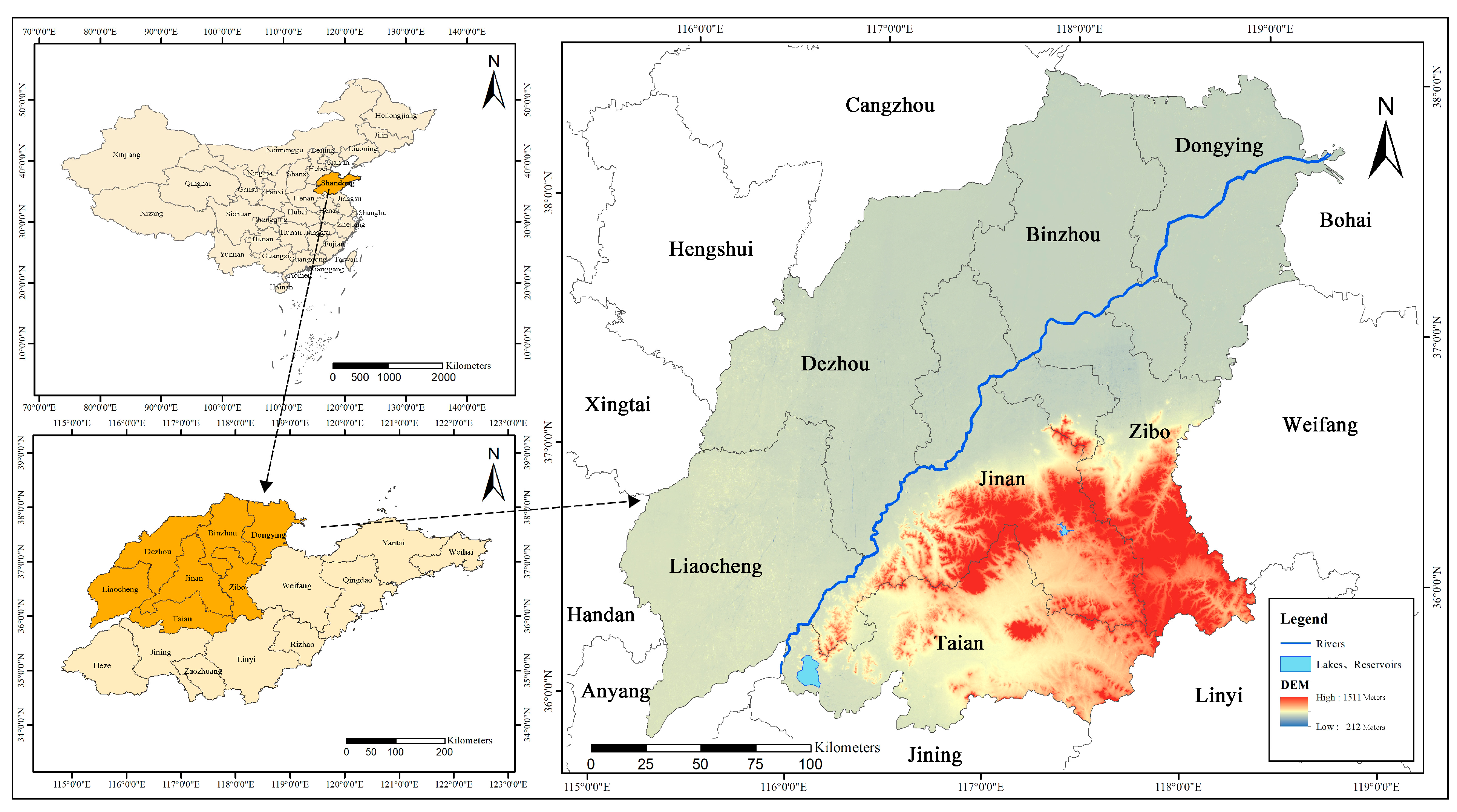
2.1. Study Area

In this study, the urban agglomeration in the Shandong section of the lower Yellow River in China was selected as the research area. This area was defined according to actual administrative boundaries, encompassing seven prefecture-level cities—Liaocheng, Tai’an, Jinan, Dezhou, Binzhou, Zibo, and Dongying—and 55 county-level administrative regions (including municipal districts) under their jurisdictions, covering an overall area of 59,100 square kilometers (Figure 1). As of 2020, the region’s total population was 37.1156 million, which is 2.63% of the country’s total population, and heavily urbanized. The research region has a diverse terrain, including plains, mountains, and hills. The landscape is high in the southeast and flat in the northwest, with elevations ranging from −212 to 1511 m. The Yellow River’s lower reaches have a high sediment concentration, making the riverbed rise progressively and the channel susceptible to siltation. These factors increase the possibility of a flood disaster and can endanger the hydrological and ecological environments. Nevertheless, with the ongoing efforts to develop green ecological corridors along the lower Yellow River and the consistent enhancement of flood control and disaster mitigation infrastructure, the quality of the ecological environment has substantially improved, effectively ensuring ecological security.

2.2. Data Source and Processing

The study included five periods: 2000, 2005, 2010, 2015, and 2020. Remote sensing monitoring data on land use change were collected from the Data Center for Resources and Environmental Sciences, Chinese Academy of Sciences (http://www.resdc.cn, accessed on 26 March 2024), at a spatial resolution of 30 m × 30 m. The data were processed by mask extraction and clipping in ArcGIS. The land use types in each year were re-classified according to the classification system for Land Use and Land Cover Change (LUCC), and six types of land use were obtained: farmland, forestland, grassland, waterbody, construction land, and unused land. DEM data were obtained from GDEMV2 30M of Geospatial Data Cloud Platform (http://www.gscloud.cn/, accessed on 7 April 2024). Temperature and precipitation data were obtained from the Shandong statistical yearbook (http://tjj.shandong.gov.cn/col/col6279/, accessed on 8 April 2024). Population and Gross Domestic Product data were extracted from the Institute of Geographical Sciences and Natural Resources Research website (http://www.resdc.cn/, accessed on 8 April 2024) at a spatial resolution of 1 km (2000–2020). The above data were converted to the Krasovsky_1940_Albers projection coordinate system for unified spatial reference.

2.3. Intensity Analysis

Aldwaik et al. [15] proposed a method for intensity analysis based on the Markov matrix to examine the temporal and spatial shifts in land use within a designated study area, encompassing three analytical tiers: time interval, category, and transformation. This study selected five specific time points—2000, 2005, 2010, 2015, and 2020—to assess the magnitude and extent of land use changes in the Shandong region along the lower Yellow River. This analytical framework was executed in Microsoft Excel 2007 (https://github.com/ss050903/Intensity_Analysis_byMicrosoftExcel, accessed on 10 April 2024).

The time interval level allows for evaluating the rate at which land use shifts occur at predetermined intervals. The formula for its representation is as follows:

$$S_t={\displaystyle \frac{\left\{{\displaystyle \sum _{J=1}^J\left[\left({\displaystyle \sum _{i=1}^J{C}_{tij}}\right)-C_{tij}\right]}\right\}/\left[{\displaystyle \sum _{J=1}^J\left({\displaystyle \sum _{i=1}^J{C}_{tij}}\right)}\right]}{Y_{t+1}-Y_t}}\times 100\%$$

(1)

$$U={\displaystyle \frac{{\displaystyle \sum _{t=1}^{T-1}\left\{{\displaystyle \sum _{i=1}^J\left[\left({\displaystyle \sum _{i=1}^J{C}_{tjj}}\right)-C_{tjj}\right]}\right\}/\left[{\displaystyle \sum _{i=1}^J\left({\displaystyle \sum _{i=1}^J{C}_{tjj}}\right)}\right]}}{Y_T-Y_1}}\times 100\%$$

(2)

where S_t represents the overall intensity of land use change during period t, U denotes the average intensity of S_t over period t, T indicates the duration of the period, i represents the initial land utilization category at the start of t, j represents the concluding land utilization category at the end of t, and J denotes the complete variety of land use categories.

The category level can be utilized to assess the intensity of land use conversion within specific time intervals. The specific mathematical expression is as follows:

$$G_{tj}={\displaystyle \frac{\left[\left({\displaystyle \sum _{i=1}^J{C}_{tij}}\right)-C_{tjj}\right]/\left(Y_{t+1}-Y_t\right)}{{\displaystyle \sum _{j=1}^J{C}_{tij}}}}\times 100\%$$

(3)

$$L_{ti}={\displaystyle \frac{\left[\left({\displaystyle \sum _{j=1}^J{C}_{tij}}\right)-C_{tii}\right]/\left(Y_{t+1}-Y_t\right)}{{\displaystyle \sum _{j=1}^J{C}_{tij}}}}\times 100\%$$

(4)

where G_tj represents the magnitude of transition for land category j in period t while L_ti denotes the magnitude of transition for land category i over the same period.

The transformation level can be used to analyze the initiation of land use type transformation within a specific time interval. The specific mathematical expression formula is as follows:

$$R_{tin}={\displaystyle \frac{\left[\left({\displaystyle \sum _{i=1}^J{C}_{tin}}\right)-C_{tnn}\right]/\left(Y_{t+1}-Y_t\right)}{{\displaystyle \sum _{j=1}^J\left[\left({\displaystyle \sum _{i=1}^J{C}_{tij}}\right)-C_{tnj}\right]}}}\times 100\%$$

(5)

$$W_{tn}={\displaystyle \frac{\left[\left({\displaystyle \sum _{i=1}^J{C}_{tin}}\right)-C_{tnn}\right]/\left(Y_{t+1}-Y_t\right)}{{\displaystyle \sum _{j=1}^J\left[\left({\displaystyle \sum _{i=1}^J{C}_{tij}}\right)-C_{tnj}\right]}}}\times 100\%$$

(6)

$$Q_{tmj}={\displaystyle \frac{\left[\left({\displaystyle \sum _{j=1}^J{C}_{tmj}}\right)-C_{tmn}\right]/\left(Y_{t+1}-Y_t\right)}{{\displaystyle \sum _{i=1}^J\left[\left({\displaystyle \sum _{j=1}^J{C}_{tij}}\right)-C_{tim}\right]}}}\times 100\%$$

(7)

$$V_{tm}={\displaystyle \frac{\left[\left({\displaystyle \sum _{i=1}^J{C}_{tmj}}\right)-C_{tmm}\right]/\left(Y_{t+1}-Y_t\right)}{{\displaystyle \sum _{I=1}^J\left[\left({\displaystyle \sum _{i=1}^J{C}_{tij}}\right)-C_{tim}\right]}}}\times 100\%$$

(8)

where R_tim represents the conversion intensity from the type of land i to a specific land type n during period t, W_tn denotes the average conversion intensity from other land types to this specific land type n during period t, C_tin represents the conversion scale area of ground class i to specific ground class n in time t, Q_tmj denotes the conversion intensity of specific ground class m to specific ground class j in time t, V_tm denotes the average conversion intensity from land type m to land type j over t.

2.4. Ecosystem Service Supply (ESS) Calculation

Land use types were divided into farmland, forest land, grassland, water bodies, construction land, and unused land. Construction land was not considered in this assessment due to its limited contribution to ES [6]. Based on the “equivalent value of ecosystem services per unit area of Chinese ecosystem” proposed by Xie Gaudi et al. [14], we calculated the supply value of ES in the lower Yellow River region [14] using two climate productivity factors, namely, temperature and precipitation, for regional revisions to the supply value equivalent of ES in the lower Yellow River region of the Shandong urban agglomeration. The specific formula is as follows:

$$L=3000+25t+0.05t^3$$

(9)

$$V=1.05r/\sqrt{1+{\left(1.05r/L+1\right)}^2}$$

(10)

$$NPP=30\times [1-e^{-0.0000695(V-20)}]$$

(11)

$$S_q=NP{P}_a/NP{P}_q$$

(12)

$$E_x=E_y\times S_q$$

(13)

$$ESSV={\displaystyle {\sum }_i^n}{A}_i\times E_x$$

(14)

Considering factors such as the yearly mean temperature (t, °C), average annual rainfall (r, mm), annual average evaporation (L, mm), and annual actual evaporation (V, mm) along with a climate contrast coefficient (S_q), we calculated the local climate’s overall production capacity (NPP_a) and compared it with the national standard (NPP_q). We also calculated the economic value of the unit equivalent factor in the study area (E_x, Yuan·hm⁻²) related to the national average (E_y, Yuan·hm⁻²). Finally, we determined the ESSV (Yuan) of the region. This comprehensive model accounted for various types of land usage (i), including farmland, forestland, grassland, water bodies, construction land, and unused land (n represents the total number of categories considered). The area allotted to each land category (Ai) is an important factor in the computation. According to the above calculation, the climate difference indexes, S_q, of the study area for the years 2000, 2005, 2010, 2015, and 2020 were 0.36, 0.49, 0.41, 0.39, and 0.45, respectively. The average value, 0.43, was the climate productivity from 2000 to 2020. The unit ESS equivalent factor in the research region had an economic value of 189.21 Yuan·hm⁻². Thus, the ESSV per unit area within the research area was calculated (

Table 1. Ecological service supply value per unit of the study area.

Primary Type	Secondary Type	Farm	Forest	Grassland	Wetlands, Rivers, and Lakes	Desserts
	Land Use	Farmland	Forestland	Grassland	Waterbody	Unused Land
Supply services	Food production	209.07	47.77	44.15	123.93	0.95
	Raw material production	46.36	109.74	64.96	69.06	2.84
	Water resources supply	−246.91	56.76	35.95	1029.28	1.89
Regulatory services	Gas regulation	168.39	360.91	228.31	252.59	12.30
	Climate regulation	87.98	1079.90	603.57	557.21	9.46
	Environment purification	25.54	316.45	199.30	865.62	38.79
	Hydrological regulation	282.86	706.69	442.11	11,964.47	22.70
Support services	Soil conservation	98.39	439.43	278.13	306.51	14.19
	Nutrient cycle maintenance	29.33	33.58	21.44	23.65	0.95
	Protection of biodiversity	32.17	400.17	252.91	985.77	13.24
Cultural services	Provision of aesthetic landscape	14.19	175.49	111.63	626.27	5.68
	Total	747.37	3726.89	2282.46	16,804.37	122.98

Note: Units, Yuan·hm⁻².

). This data served as a foundation for subsequent calculations of the spatial distribution of ESSV, assessments of ecological sensitivity, and hotspot analysis.

2.5. Sensitivity Analysis

Ecological sensitivity refers to the degree of response of the ecological environment to human activities and natural environmental changes [26]. In this study, the method for calculating ES value based on equivalent factors was employed. The precise determination of the ESSV coefficient is pivotal to ensuring the accuracy of this calculation. The coefficient of sensitivity (CS) was selected as a key indicator to assess the applicability of this value coefficient. Specifically, CS quantifies the degree to which changes in the value index influence the valuation of ES over time. The elasticity was measured by adjusting the value coefficient of ES supply up and down by 50% to determine whether the results were accurate and reliable. The specific calculation formula is as follows:

$$CS=\left|{\displaystyle \frac{\left(P_{ESS{V}_j}-p_{ESS{V}_i}\right)/P_{ESS{V}_i}}{\left(V{C}_{jk}-V{C}_{ik}\right)/V{C}_{ik}}}\right|$$

(15)

where P_ESSVj and P_ESSVi are ESSV coefficients before and after adjustment for the ecological service supply value coefficient, respectively, and VC_jk and VC_ik are the ESSV coefficients before and after adjustments are made according to land category k. If the sensitivity index (CS) exceeds 1, the ESSV is more sensitive to changes in these coefficients, which may lead to reduced accuracy or lower confidence in the conclusions. When CS is below 1, the ESSV exhibits less sensitivity to such variations, indicating higher precision and reliability of the study’s conclusions.

2.6. Cold and Hot Spot Analysis

The application of hotspot analysis is common in ecological environmental studies. In this context, hot spots and cold spots characterize high- and low-value spaces, respectively, where significant aggregation occurs. In this study, the hot spot analysis tool (Getis-Ord Gi*) in ArcGIS 10.8 was used for analysis. The Z-value represents the multiple of standard deviation, and the P-value represents the probability. Hot spot analysis tools can identify regions with statistically significant clusters within the study’s scope, illustrating the spatial correlation between land use change and ESSV. The formula is as follows:

$$G_i^{\ast }={\displaystyle \frac{{\displaystyle \sum _{j=1}^n{w}_{i,j}{x}_j-\overline{x}}{\displaystyle \sum _{j=1}^n{w}_{i,j}}}{\sigma \sqrt{n{\displaystyle \sum _{j=1}^n{w}_{i,j}^2}}-{\left({\displaystyle \sum _{j=1}^n{w}_{i,j}}\right)}^2}}$$

(16)

where G_i^* is the local autocorrelation index of region i, W_i,j is the spatial weight system of the i and j geospatial units, X_j is the ecological environment quality index, and σ is the standard deviation.

2.7. Geographic Detector

A geographic detector is a pivotal tool for elucidating the underlying factors that propel the variation in explained variables within a spatial context [27]. By meticulously analyzing spatial differentiation, this technique is adept at quantifying the profound influence that these drivers exert on the spatial differentiation of the ESSV. We carefully assessed the current situation prevailing in the study area. According to the analysis, two categories of seven different driving factors were identified. The natural driving factors were temperature, precipitation, and NDVI; human-driven factors included GDP, POP, night light intensity, and distance from the Yellow River. An approach known as “Natural Breaks” was employed to categorize and divide the data used by the driving factors into ten discrete levels. The precise formula is as follows:

$$q=1-{\displaystyle \frac{{\displaystyle \sum _{h=1}^L{N}_h{\delta }_h^2}}{N{\delta }_h^2}}$$

(17)

where the variable q shows the influence exerted by a specific driving factor under investigation; σ² and σ_h² denote the variances observed within the larger research region and the more narrowly defined sub-area, respectively; N and N_h represent the sample sizes pertaining to the overall study area and the delineated sub-area, respectively. It is vital to keep in mind that the value of q is constrained within the interval [0, 1]. A higher value of q signifies that the driving factors possess considerable explanatory power for the ESSV being analyzed. Conversely, lower values of q denote diminishing influence.

3. Results

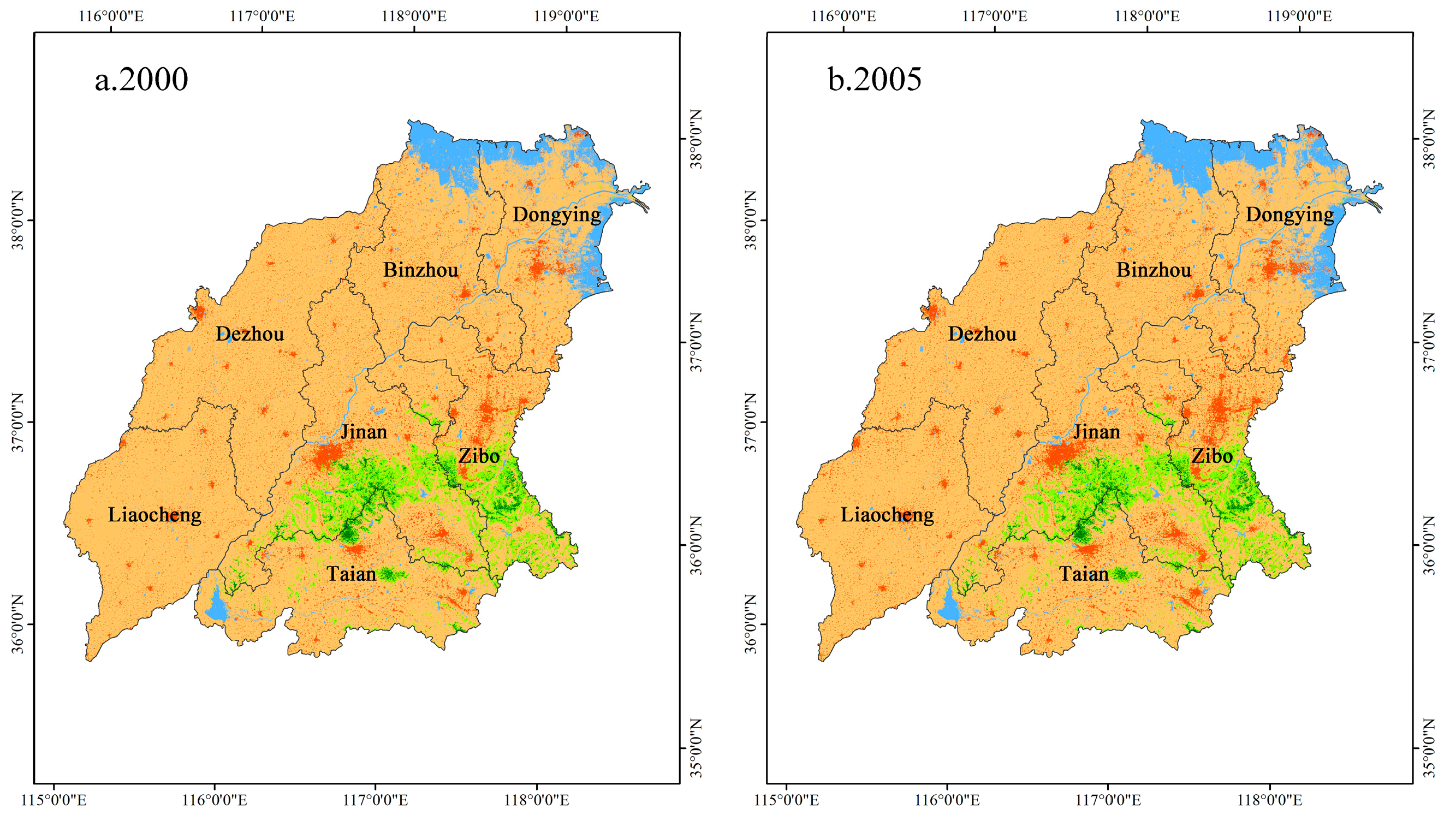
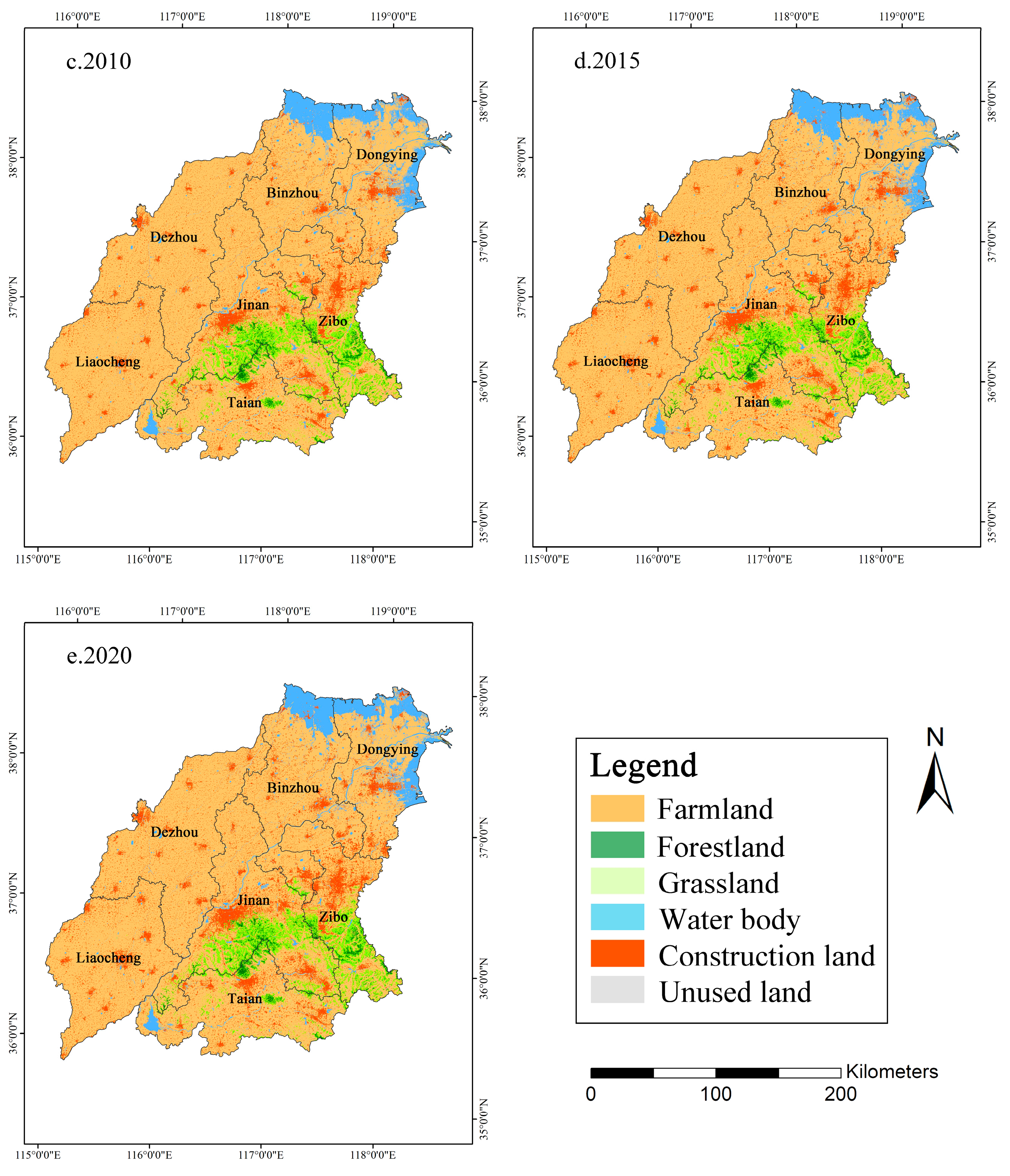
3.1. Spatiotemporal Evolution of Land Use

Farmland made up the largest area within the study site, accounting for 78.53% of the total area in 2000. Next was construction land, accounting for 11.24% in 2020. The main changing trend in different land use types in the research area between 2000 and 2020 was that the area covered by farmland, grassland, and unused land gradually decreased, while the area covered by forestland, construction land, and waterbodies gradually increased (Figure 2 and Figure 3). Among them, the decrease in farmland was the largest, at 7.32%, and the increase in construction land was the largest, at 76.59%, while the overall change in the waterbody area was the smallest. Mount Tai stands at the intersection of Jinan, Zibo, and Tai’an in the southwest of the study area. Rugged and mountainous landscapes characterize the terrain. The primary land use types are forestland and grassland, which showed a moderately increasing trend from 2000 to 2020. Waterbodies are mainly distributed along the Yellow River, forming a convergence at the estuary, with the overall area increasing along the river and the coast. Affected by the location of central urban areas of cities and counties in the study area, construction land is distributed in a point pattern, with the area expanding outward from 2000 to 2020. The area delineated for urban development within the boundaries of Jinan City and Zibo City showed a gradual planar distribution with progressive social and economic development. The trend of the change in unused land area was statistically nonsignificant.

The rapid expansion of construction land primarily encroaches on farmland areas, reflecting the process of rapid urbanization. However, high-intensity human activities have led to environmental degradation and increased ecosystem vulnerability. The transformation of farmland into waterbodies within the Yellow River Basin is a testament to the success of integrated approaches to ecological management (Figure 2 and Figure 3). The regional and temporal pattern of land use conforms to natural and societal conditions.

3.2. Figures, Tables, and Schemes

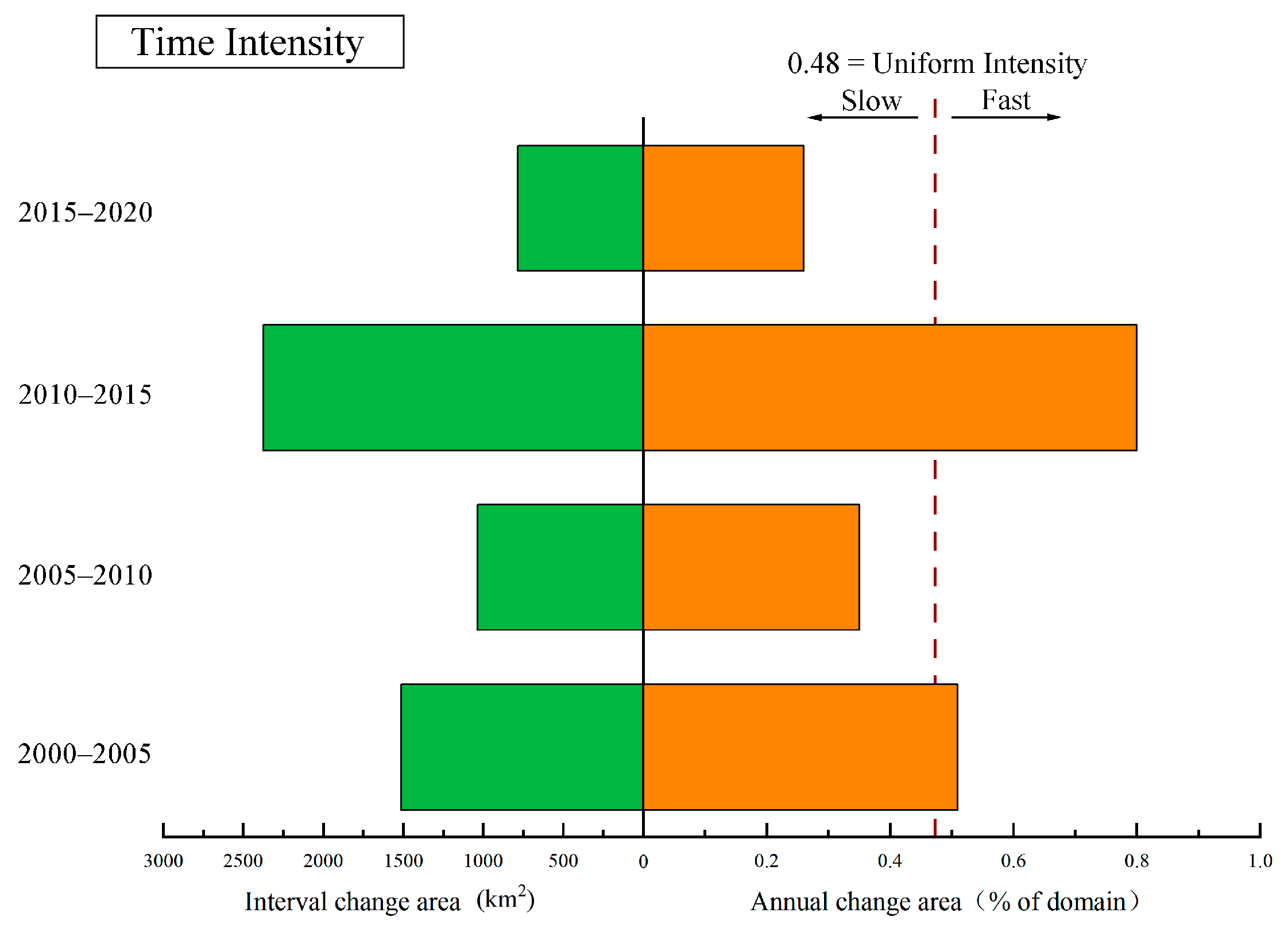
3.2.1. Interval Level

In 2000–2005 and 2010–2015, the average annual change in area accounted for 0.51% and 0.80% of the study area, and overall development showed an accelerating trend. In 2005–2010 and 2015–2020, the average annual change in area accounted for 0.35% and 0.26% of the study area, and development was relatively slow. The acceleration in development from 2000 to 2005 was closely related to the rapid development of the urban economy. The area and rate of land change reached a maximum between 2010 and 2015, attributed to the policy of the connection between the increase in urban land and the decrease in rural construction land (Figure 4).

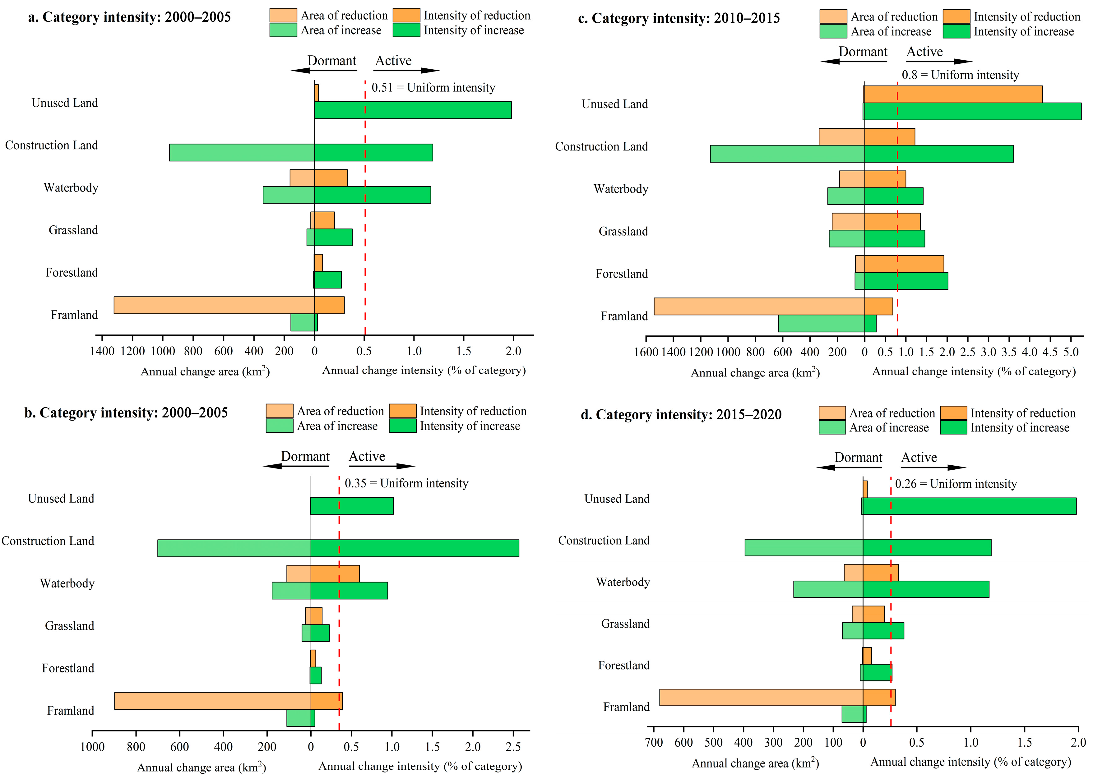
3.2.2. Category Level

In 2000–2005, the loss intensities for all types of land were small and did not exceed the average intensity; the largest area lost was farmland (Figure 5). The income intensity of waterbody, construction land, and unused land areas was greater than the average value, with unused land yielding the highest income. Although forestland and grassland have a certain intensity of return, they were not greater than the average.

When examining the data from 2000 to 2005 alongside that from 2005 to 2010, the rate of change for different types of land use showed a remarkable uptick in the later timeframes. Except for farmland, the degree of loss and gain of other land categories surpassed the average levels during this period. This was particularly notable for unoccupied land, which experienced the highest intensity of change. The loss of farmland was first, followed by the highest gain of construction land, reflecting the rising trend of urbanization. In terms of the unbalanced difference between “gain” and “loss” of land use type, the performance in 2005–2010 was particularly outstanding. From 2010 to 2015, the differences were primarily in farmland, construction land, and waterbody areas. The income intensity and construction land area reached a peak, coinciding with the most substantial decline ever seen in farmland areas. Between 2015 and 2020, the income intensity of unused land, waterbody, and construction land areas increased, while the largest loss in area was farmland. Based on the data from 2000 to 2020, the gain intensity for waterbody, construction land, and unused land areas was generally higher than the average intensity, while the area of farmland lost was highest. Other terrestrial classes show unstable change patterns, indicating uneven and dynamic changes in local classes.

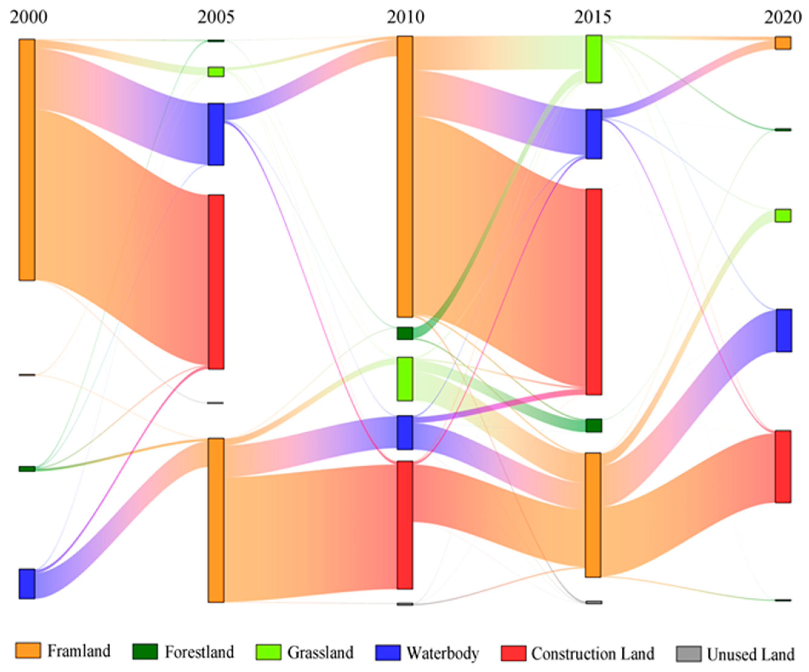
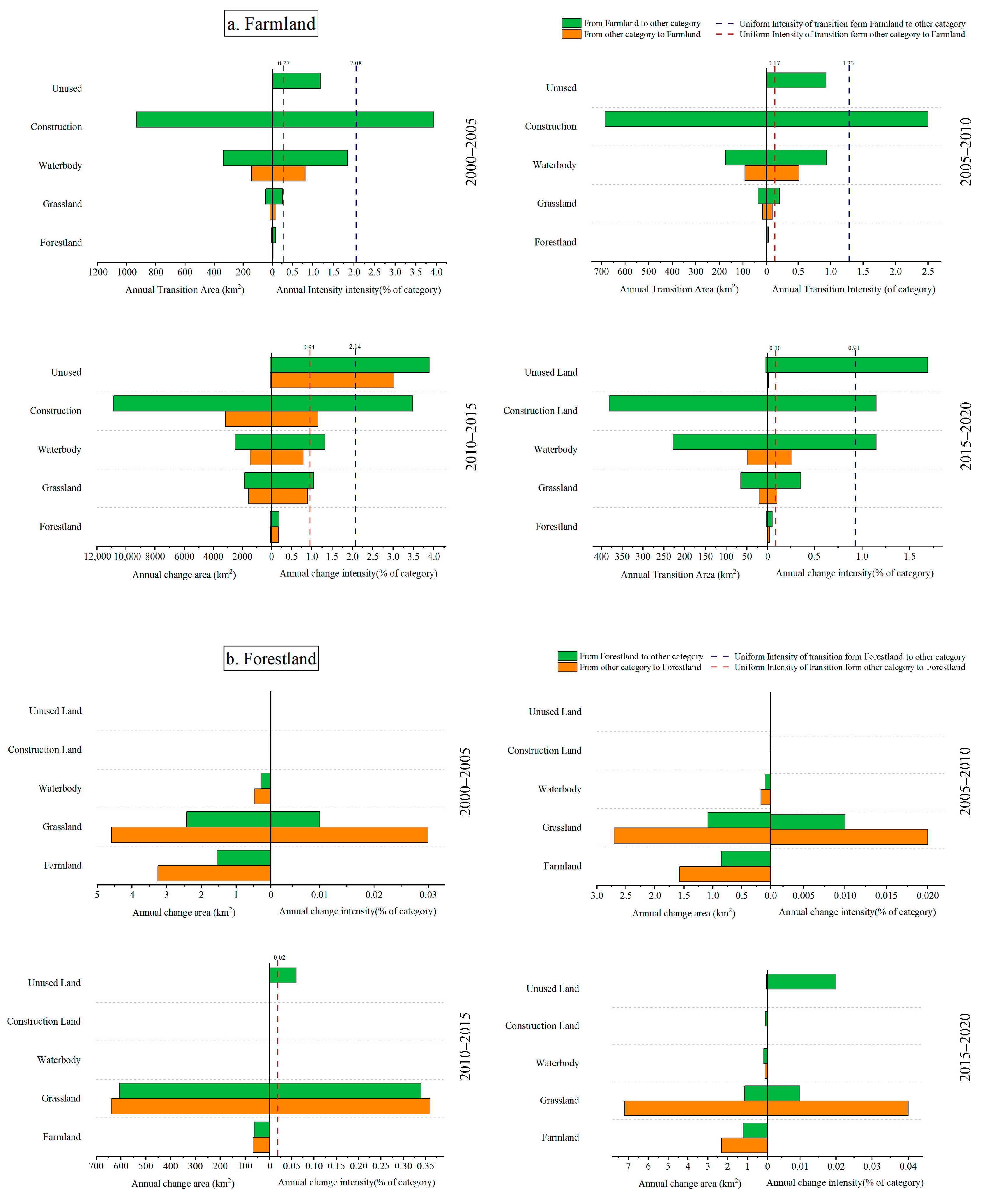
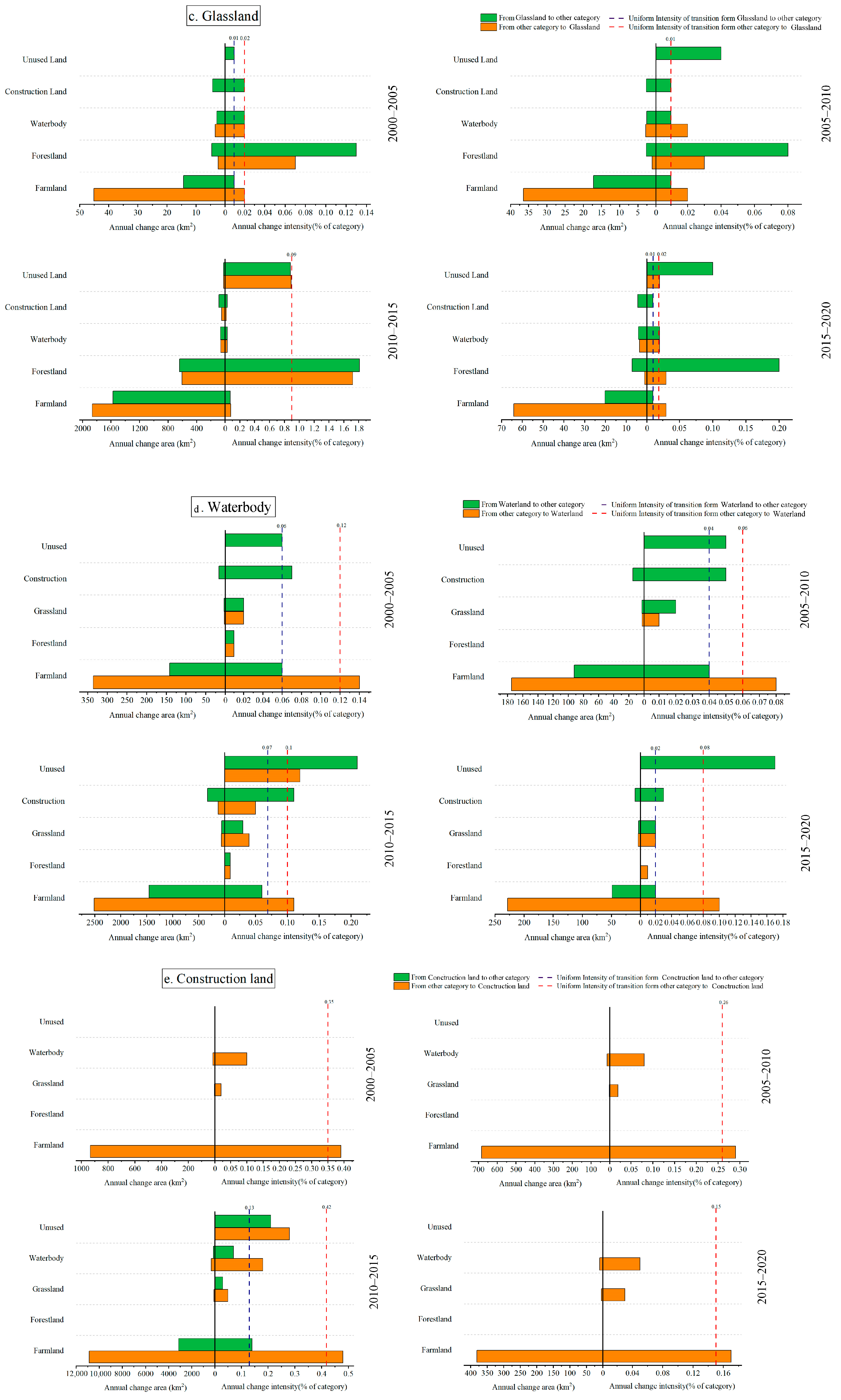
3.2.3. Transformation Level

The trend of the evolution of land use types showed significant changes during the four time intervals. Judging from the pattern of reduction at the transformation level, the intensity of farmland conversion (Figure 6a) into construction land during the four time intervals exceeded the average intensity, indicating the expansion of construction land on a big scale during this period, occupying a portion of the farmland. The intensity of the transformation into waterbodies gradually increased due to the development of the Yellow River regulation action and the consolidation of the later results. From 2010 to 2020, the conversion intensity to unused land increased more than the average intensity due to the accelerated urbanization process caused by the loss of rural labor and land wastage.

From the perspective of the increasing pattern of transformation levels, taking the waterbody as an example (Figure 6d), the intensity of the transformation from farmland to waterbody was highest in the four time intervals, exceeding the average intensity, while the other land classes had less than the average intensity, except for unused land, which showed a larger transformation intensity in 2010–2015. With the development of ecological remediation actions in the coastal areas of Binzhou City and Dongying City in the north, farmland is being continuously transformed into wetlands, further improving the ecological environment.

The conversion between forestland (Figure 6b) and grassland (Figure 6c) was frequent and more intense than average, reflecting the effectiveness of ecological restoration and land management. Simultaneously, farmland to grassland and forestland conversion occurred; however, the scale of this transition was not constant. It correlated directly with initiatives such as ‘Farmland to Forest’ and ‘Farmland to Grassland’ policies and environmental restoration efforts along the banks of the lower Yellow River.

The transfer of land use types in the study area was mainly concentrated in 2000–2015. During this period, the conversion of land use type was manifested as a significant increase and decrease in construction land and farmland, respectively. This trend was directly correlated with the heightened demand for construction sites during the urban development phase and the enforcement of the Policy on the “Connection between the Increase of Urban Land and the Decrease of Rural Construction Land”. The period from 2010 to 2015 was transitional, with a two-way transition trend in all land use types. Urban development stabilized gradually from 2015 to 2020, the area converted to construction land decreased, and the area covered by waterbodies showed an increasing but nonsignificant trend.

3.3. Analysis of the Change in ESSV

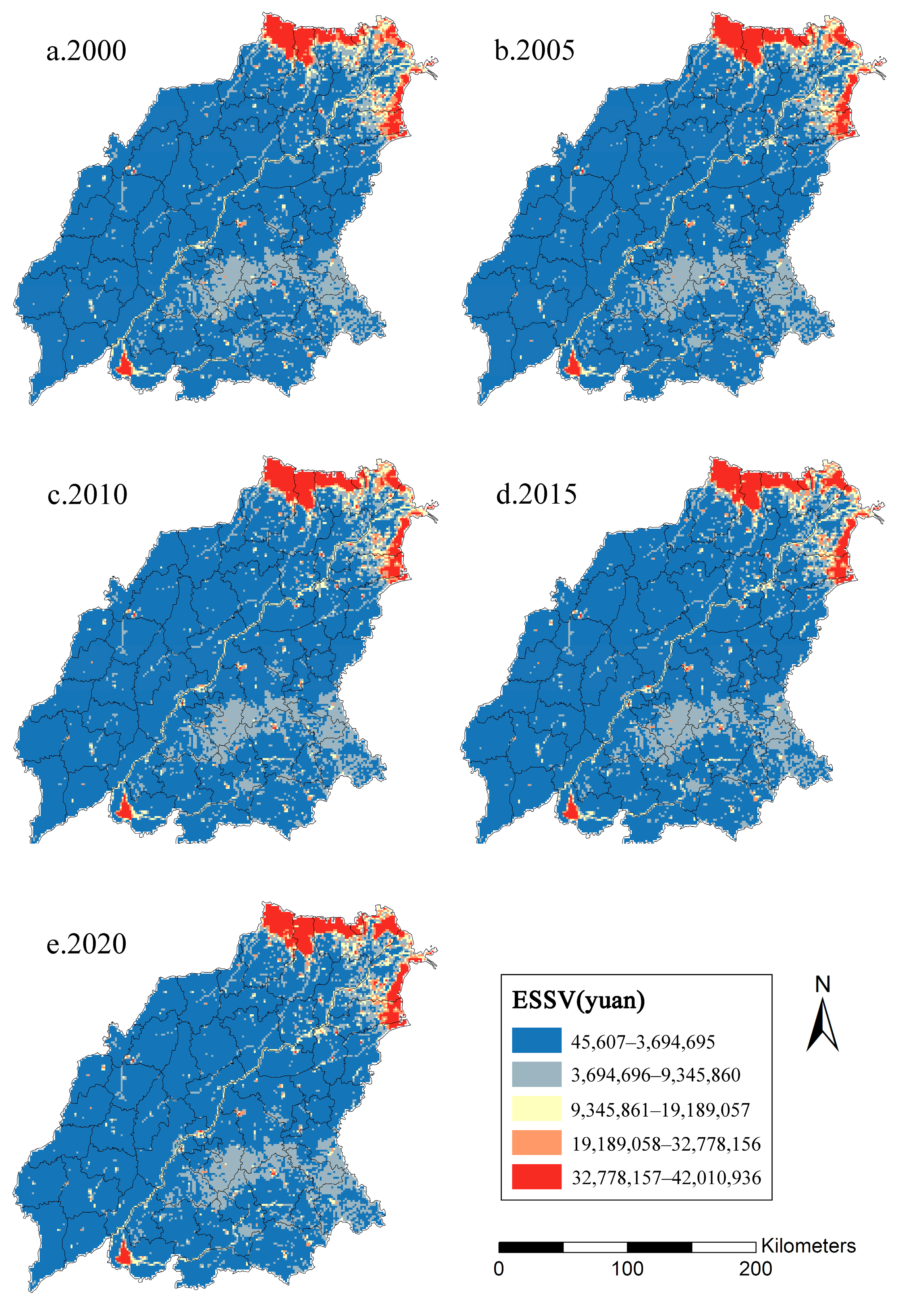
3.3.1. Spatial and Temporal Patterns of ESSV

ESSV increased steadily between the years 2000 and 2020; the corresponding figures are 8.497 billion Yuan, 8.833 billion Yuan, 8.935 billion Yuan, 8.938 billion Yuan, and 11.142 billion Yuan. During the period from 2015 to 2020, the growth rate in ESSV was particularly significant, highlighting the positive effect of the study area in enhancing the ESSV. From the perspective of land use types, apart from continuous growth in waterbodies, the ESSV of other land use types decreased, mainly because farmland, grassland, waterbodies, unused land, and various types of lands were lost to urban development. The ESSV of waterbodies dominates the study area with the largest contribution, accounting for 59.42% in 2020; this is followed by farmland, which accounts for 25.92%. This change was mainly attributed to the effective implementation of comprehensive remediation actions in the lower Yellow River, which has significantly maintained and improved the ecological environment in the study area.

This study used a 1.5 km × 1.5 km grid to employ spatial arrangement and visual manifestation of ESSV. The ESSV of the various land use categories in every grid was summed, and the resulting spatial distribution map of ESSV was classified into five groups using the natural breakpoint approach (Figure 7). The blue and red trends represent the “low-value areas” and the “high-value areas”, respectively. The “low-value areas” are mainly located in Liaocheng City, Dezhou City, and Tai’an City, with plain terrain as the main land use type, while the “high-value areas” are located along the Yellow River and in the northern estuary area, with waterbody as the main land use type. Furthermore, the mountainous and hilly areas in the southwest exhibit relatively high ESS values, primarily attributed to abundant forestland and grassland resources. On the whole, the spatial distribution of ESSV aligns closely with that of individual land use within each cell on the map. The ESSV of a mixed grid containing multiple land use types shows a spatial transition.

The temporal and spatial characteristics of ESSV in the lower Yellow River region in 2000–2020 were further analyzed in 55 counties (including municipal districts) in the study area. The spatial distribution of ESSV changed little from 2000 to 2005, mainly attributed to the increase in the waterbody area in the Dongying Estuary area, northern Lijin County, Dongying District, and western Kenli District. There was no significant change in the spatial distribution of ESSV from 2005 to 2010. From 2010 to 2015, the waterbody area in Dongying Hekou District and northern Lijin County continued to increase. The management along the Yellow River in the Tianqiao District of Jinan began to take effect, and ESSV increased. From 2015 to 2020, with comprehensive supervision of soil and water conservation efforts in the Yellow River Basin, the ESSV of the area along the Yellow River significantly increased. The increase in the area occupied by waterbodies in the estuary in Dongying City has contributed to the ESSV reaching its highest point in the past years.

3.3.2. Sensitivity Analysis of ESSV

In the analysis of the plus or minus 50% adjustment for the ESSV coefficients of all types of land use in the study area, the sensitivity index (SI) of ESSV to the value coefficient remained stable below 1 in five consecutive interval years (

Table 2. Sensitivity index of ESSV in the study area.

Ecosystem	VC	2000	2005	2010	2015	2020	2000–2020
Framland	VC ± 50%	0.255	0.244	0.238	0.232	0.223	−0.032
Forestland	VC ± 50%	0.019	0.018	0.018	0.018	0.018	−0.001
Grassland	VC ± 50%	0.057	0.057	0.057	0.057	0.056	−0.002
Waterbody	VC ± 50%	0.419	0.431	0.437	0.443	0.453	0.034
Unused Land	VC ± 50%	0.000	0.000	0.000	0.000	0.000	0.000

). This stable trend strongly suggests that ESSV in the study area was less sensitive to fluctuations in the value coefficient, thus improving the reliability and robustness of the results. Upon closer inspection, it was clear that the value associated with the ESSV for the waterbody, represented by the CS value, increased gradually over time. In contrast, the CS value for farmland decreased year after year. Although the CS values for woodland and grassland areas decreased, the changes were nonsignificant. Combined with recent water protection policies and actions implemented in the Yellow River Basin, this shift underscores the constructive influence of ecological safeguarding strategies on the overall worth of ecosystem services, particularly in protected water areas.

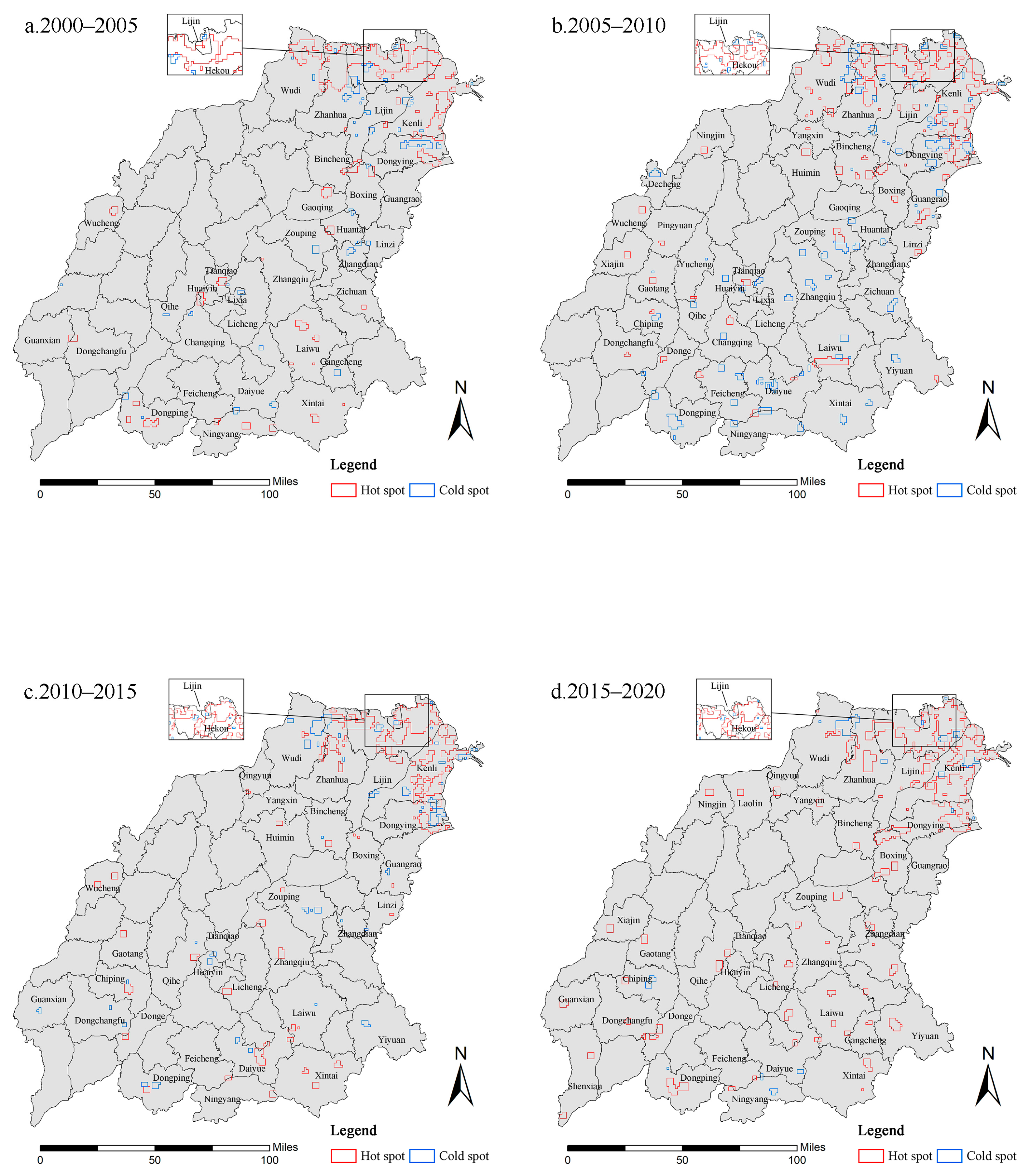
3.3.3. Cold and Hot Spot Analysis of ESSV

The cold and hot spot analysis method overlays ESSV in the study area, revealing its spatial clustering characteristics to explore the interrelation between ESSV and land use change in depth. From 2000 to 2020, the ESSV areas were concentrated in the northern Yellow River estuary and the surrounding areas, while the cities and counties in the region exhibited a more dispersed distribution (Figure 8).

Significant patterns and trends can be observed in the spatial distribution of ESSV in the study area from 2000 to 2020. From 2000 to 2005, ESSV hot spots were mainly focused on the northern part of the study area, including Hekou County in Dongying City, Diaokou Township located in Lijin County’s northern enclave, as well as the northern regions of Wudi County and the northeastern portion of Kenli County. The emergence of these hot spots was mainly due to the transformation of farmland to waterbodies, significantly improving the ESSV of the region. The cold spots were concentrated in the Zhanhua District of Binzhou City, Zouping City, Dongying City, and Zhangdian District of Zibo City. This is attributed to the conversion of extensive farmland and waterbodies into construction land, leading to prominent cold spots. From 2005 to 2010, the range of ESSV hot spots expanded significantly, covering 28 northern counties in the study area and forming a point-like distribution in the western and southern counties such as Xiajin County, Wucheng County, and Gaotang County. Simultaneously, the number and extent of cold spots also increased in the study area’s center and southern regions, mostly due to the destruction and replacement of the natural ecosystem caused by high-intensity building development. From 2010 to 2015, affected by the Yellow River basin protection policy, hot spots such as the coastal estuary area, Kenli County, and Lijin County showed a trend of connecting points, and the number and scope of cold spots decreased, concentrated in Dongying City, Wudi County, and Huaiyin District of Jinan City. The overall development of the city gradually stabilized. From 2015 to 2020, the hot spots in the northern part of the study area were distributed planarly, and their range and number increased, illustrating the importance of the transformation of farmland into waterbodies in terms of ESSV.

3.4. Analysis of Spatial Differentiation of ESSV

3.4.1. Single-Factor Detection Analysis

Seven driving factors were chosen as independent variables from natural environmental and socioeconomic factors, with ESSV as the dependent variable. These factors were population (X1), average land GDP (X2), precipitation (X3), air temperature (X4), normalized vegetation index (X5), night light index (X6), and distance from the Yellow River (X7). They were selected as independent variables from natural environmental factors and socio-economic factors. Quantitative analysis was conducted using the “Factor Detector” and “Interaction Detector” functions in the GeoDetector tool. Figure 9 depicts explanatory power (q) values for ESS drivers from 2000 to 2020. In terms of overall influence, NDVI, population, temperature, and precipitation were the most influential factors from 2000 to 2020; GDP, night light index, and distance from the Yellow River exerted a minor effect on ESSV. Except for the population with the largest q value affecting the ESSV value in 2000, the largest q value from 2005 to 2020 was NDVI, reflecting that the rapid economic and social development caused by population growth around the year 2000 greatly impacted ESSV. After 2005, the ES value changed mainly due to the influence of the natural factor, NDVI.

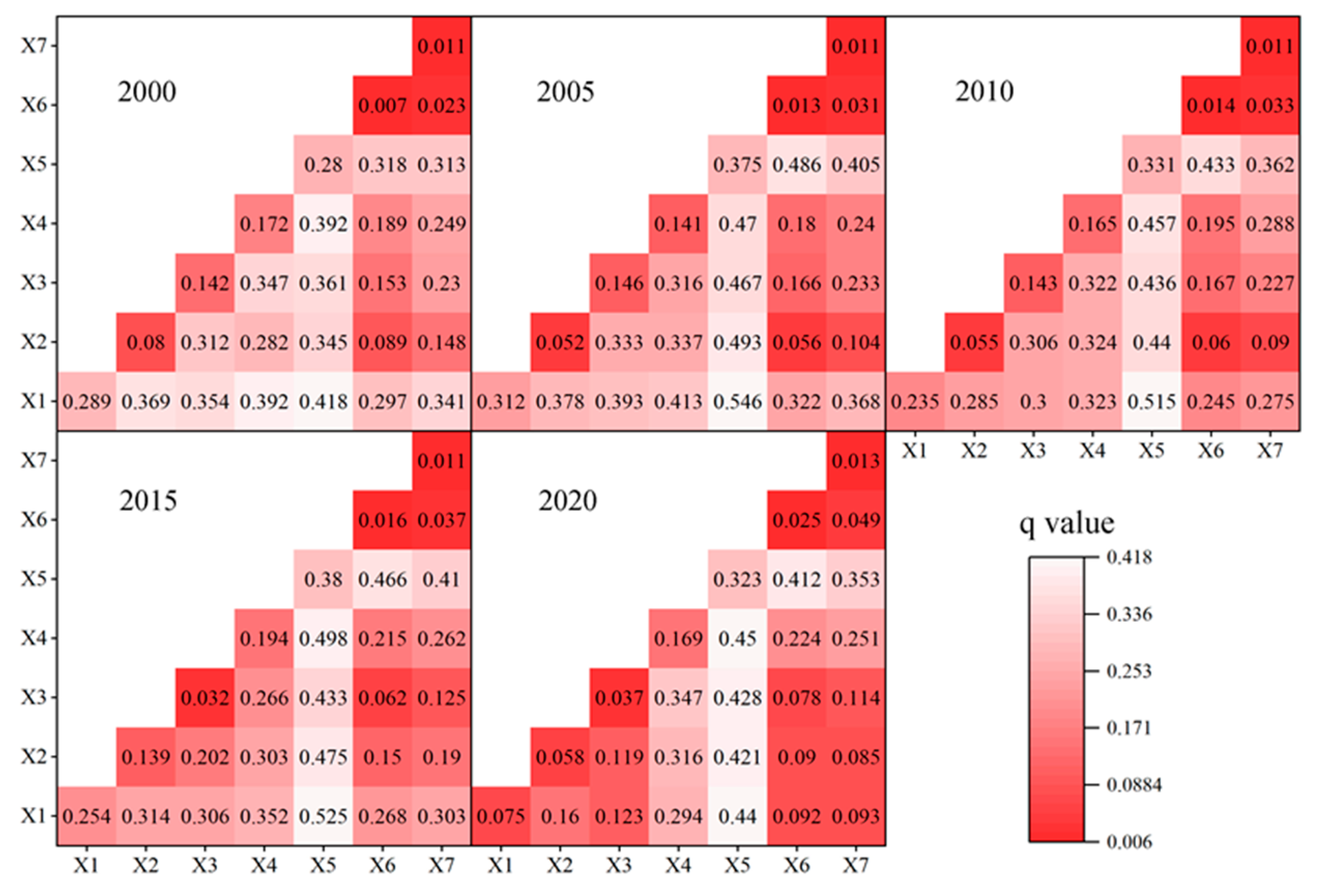
3.4.2. Detection and Analysis of Factor Interactions

From 2000 to 2020, each driving factor’s interaction with ESSV showed nonlinear enhancement and double enhancement, with no independent interaction or nonlinear weakening, demonstrating that, rather than being the result of a single component, the combined effects of several driving factors caused spatial differentiation in ESSV in the research area (Figure 10). The explanatory power of the interaction of driving factors in different years was different. The interaction between NDVI and the population exhibited its most pronounced influence from 2000 to 2015, peaking at 0.546 in 2005. In contrast, the interaction between NDVI and temperature showed the highest impact in 2020, reaching a high of 0.45. Simultaneously, the explanatory power of population (POP) and per capita GDP factors increased, indicating that natural factors and social factors worked together to change the ESSV. Because of the influence of population policy and the Yellow River control action in 2000–2020, the interplay of NDVI, POP, and other elements greatly affected ESSV. A comprehensive analysis of the interaction of POP, per capita GDP, precipitation, air temperature, normalized vegetation index, night light index, distance from the Yellow River, and changes in the value of the single explanatory power q suggests that future changes in ESSV in the study area will be a result of multi-factor synergistic influences.

4. Discussion

Land use dynamics in urban clusters along the lower Yellow River changed substantially between 2000 and 2020. Rapid urbanization coupled with the profound effects of human actions on land resources led to a steady decline in farmland, with increasing conversion into construction land and waterbodies. Specifically, the area covered by construction land experienced significant growth during this period, aligning with the accelerated urbanization observed in the lower Yellow River region from 1990 to 2020, in line with the findings documented by Li Xin et al. [28]. This growth reflects substantial demand for land resources driven by urbanization and industrialization processes. With the active promotion of ecological protection policies, the area covered by water bodies has shown a steady upward trend [29], consistent with the implementation of ecological political work in the region. Compared with waterbody and construction land areas, the changes in grassland and forestland areas are relatively weak and there is a certain conversion phenomenon between them. The growth in forestland is mainly due to the conversion of grassland, while the reduction in grassland is partly due to the conversion of farmland and unused land. The findings that farmland, unused land, and grassland are shrinking while construction, waterbody, and forestland areas are increasing align with the conclusions of Zhang Pengyan et al. [25].

The analytical framework for land utilization intensity adopts a hierarchical, top-down approach, which is essential for attaining a comprehensive, systematic grasp of land use transformation dynamics. Distinct from alternative methodologies, this intensity-based analysis boasts heightened precision in quantifying the internal reconfigurations within regional urban land use categories and the subsequent impacts of human endeavors. It elucidates the intricate interplay between alterations in urban land use patterns, the progression of urbanization, and the implementation of ecological conservation strategies along the Shandong stretch of the lower Yellow River. This point has been verified by Ding Xue et al. [30]. While intensity analysis has significant advantages, it falls short of accurately capturing intensity changes across all spatial dimensions. This constraint limits the knowledge of how spatial proximity drives changes in land use; therefore, future research should address this difficulty to provide more comprehensive knowledge of the spatial dynamics underpinning land use changes.

Spatio-temporal changes in land use further affect the spatial differentiation of ESSV. ESSV increased continuously from 2000 to 2020; however, the growth rate was characterized by heterogeneity. This finding differs from the results of Liu Chang et al. [31]. This may be due to the difference in the definition of the study area; the former covers the entire Henan and Shandong provinces in the lower reaches of the Yellow River, while the present study focuses on some cities in Shandong Province in the lower reaches of the Yellow River. This difference shows heterogeneity in the spatial distribution of ESSV. It underscores the need to consider the specificities of geographical areas when seeking a thorough comprehension of environmental conservation efforts and formulating strategic plans aimed at fostering sustainable growth. Compared with relevant studies in the Shandong section of the Yellow River Basin [32], both discussed the relationship between land use change and ESSV in the study area using a land use transfer matrix and analysis of changes in ESSV. In this study, land intensity analysis, ecosystem service supply value cold and hot spot analysis, and geographical detector analysis are added. It is useful to investigate the connection between changes in land use type and ecological responses temporally and spatially, in addition to the influencing factors.

Comparison of land use status and ESSV in the lower Yellow River shows that the timeliness of this study has some limitations. The lack of data before the year 2000 limits complete understanding of the region’s long-term changes in land use and their feedback mechanisms to ecosystem service functions. Future studies should consider expanding the time horizon to more fully understand and assess land use dynamics and their potential impacts on ESSV in the lower Yellow River region to enhance the comprehensiveness and depth of the study. The methods of spatial dynamic analysis of changes in land use should also be explored so that the change in each level of intensity can be clearly expressed in spatial dimensions to reveal the impact of spatial adjacency on the changes in land use.

5. Conclusions

Farmland in the study area shrank from 2000 to 2020, while construction land increased steadily. The change in the intensity of land use peaked between 2005 and 2010. The ESSV for the study area has continued to increase over the last two decades, increasing to 31.13% by 2020 with an overall revenue of 11.142 billion Yuan. In terms of spatial distribution, the “low-value areas” of ESSV change were primarily concentrated in western and southwestern regions dominated by plain terrain, where farmland was the predominant land use type. The “high-value areas” were distributed in regions along the Yellow River, the northern estuary, and the southeastern mountainous and hilly areas where land use is primarily waterbody, forestland, and grassland. The geographical distribution of low- and high-value ESSV areas crossed the boundaries of traditional administrative divisions. This spatial pattern reveals the regional characteristics of ESSV and has important significance and reference value for promoting regional coordination and comprehensive management of ecological protection policies. Further analysis showed that the ESSV cold and hot spots were concentrated in the northern estuary and the Yellow River, flowing through the area with a spot-like distribution. The spatial distribution of the hot spots tended to gradually concentrate, forming a continuous surface area, while the number of cold spots increased first and then decreased under the influence of urban economic development and subsequent ecological management measures. The conversion of different types of land to construction land and waterbodies was the most important land use transformation mode in the cold and hot spots in terms of ESSV, and waterbodies were the most sensitive to changes in ESSV. Considering various influencing factors, including natural factors and human activities, the ESSV of the study area exhibited significant spatial differences, particularly in the interaction between NDVI and population. Our findings provide a strong scientific basis for formulating more targeted ecological protection strategies in the future, conducive to promoting regional sustainable development.

References

1. Burkhard, B.; Kroll, F.; Nedkov, S.; Müller, F. Mapping Ecosystem Service Supply, Demand and Budgets. Ecol. Indic. 2012, 21, 17–29. [Google Scholar] [CrossRef]
2. Chen, Z.; Zhang, Q.; Li, F.; Shi, J. Comprehensive Evaluation of Land Use Benefit in the Yellow River Basin from 1995 to 2018. Land 2021, 10, 643. [Google Scholar] [CrossRef]
3. Krugman, Y. Increasing Returns and Economic Geography. J. Political Econ. 1991, 99, 483–499. [Google Scholar] [CrossRef]
4. Wang, B.; Yang, X.; Dou, Y.; Wu, Q.; Wang, G.; Li, Y.; Zhao, X. Spatio-Temporal Dynamics of Economic Density and Vegetation Cover in the Yellow River Basin: Unraveling Interconnections. Land 2024, 13, 475. [Google Scholar] [CrossRef]
5. Liu, M.; Xiong, Y.; Zhang, A. Multi-scale telecoupling effects of land use change on ecosystem services in urban agglomera-tions—A case study in the middle reaches of Yangtze River urban agglomerations. J. Clean. Prod. 2023, 415, 13787. [Google Scholar] [CrossRef]
6. Gyurkovich, M.; Dudzic-Gyurkovich, K.; Matusik, A.; Racoń-Leja, K. Vistula River Valley in Cracow: From an Urban Barrier to a New Axis of Culture in the Scale of the City. ACE Archit. City Environ. 2021, 15, 9913. [Google Scholar] [CrossRef]
7. Chang, L.; Shuheng, Z.; Rong, Z.; Xinhan, Q.; Guanglong, D. Land Space Dynamic Changes and Cross-Sensitivity of Ecological Service Function in the Lower Yellow River Reaches. J. Agric. Resour. Environ. 2023, 40, 976–992. [Google Scholar] [CrossRef]
8. Cui, J.; Zhu, M.; Liang, Y.; Qin, G.; Li, J.; Liu, Y. Land Use/Land Cover Change and Their Driving Factors in the Yellow River Basin of Shandong Province Based on Google Earth Engine from 2000 to 2020. ISPRS Int. J. Geo-Inf. 2022, 11, 163. [Google Scholar] [CrossRef]
9. Costanza, R.; d’Arge, R.; De Groot, R.; Farber, S.; Grasso, M.; Hannon, B.; Limburg, K.; Naeem, S.; O’Neill, R.V.; Paruelo, J.; et al. The Value of the World’s Ecosystem Services and Natural Capital. Nature 1997, 387, 253–260. [Google Scholar] [CrossRef]
10. Bateman, I.J.; Harwood, A.R.; Mace, G.M.; Watson, R.T.; Abson, D.J.; Andrews, B.; Binner, A.; Crowe, A.; Day, B.H.; Dugdale, S.; et al. Bringing Ecosystem Services into Economic Decision-Making: Land Use in the United Kingdom. Science 2013, 341, 45–50. [Google Scholar] [CrossRef]
11. Hasan, S.S.; Zhen, L.; Miah, M.G.; Ahamed, T.; Samie, A. Impact of Land Use Change on Ecosystem Services: A Review. Environ. Dev. 2020, 34, 100527. [Google Scholar] [CrossRef]
12. Zhang, C.; Zhao, L.; Zhang, H.; Chen, M.; Fang, R.; Yao, Y.; Zhang, Q.; Wang, Q. Spatial-Temporal Characteristics of Carbon Emissions from Land Use Change in Yellow River Delta Region, China. Ecol. Indic. 2022, 136, 108623. [Google Scholar] [CrossRef]
13. Zhao, Q.; Wen, Z.; Chen, S.; Ding, S.; Zhang, M. Quantifying Land Use/Land Cover and Landscape Pattern Changes and Impacts on Ecosystem Services. Int. J. Environ. Res. Public Health 2020, 17, 126. [Google Scholar] [CrossRef]
14. Qiao, W.; Sheng, Y.; Fang, B.; Wang, Y. Land use evolution information mining in highly urbanized areas based on transfer matrix: A case study of Suzhou, Jiangsu Province. Geogr. Res. 2013, 32, 1497–1507. [Google Scholar]
15. Aldwaik, S.Z.; Pontius, R.G., Jr. Intensity Analysis to Unify Measurements of Size and Stationarity of Land Changes by Interval, Category, and Transition. Landsc. Urban Plan. 2012, 106, 103–114. [Google Scholar] [CrossRef]
16. Gaodi, X.; Lin, Z.; Chunxia, L.; Yu, X.; Wenhua, L.I. Applying Value Transfer Method for Eco-Service Valuation in China. J. Resour. Ecol. 2010, 1, 51–59. [Google Scholar] [CrossRef]
17. Xie, G.; Zhang, C.; Zhang, L.; Chen, W.; Li, S. Improvement of the Evaluation Method for Ecosystem Service Value Based on per Unit Area. J. Nat. Resour. 2015, 30, 1243–1254. [Google Scholar] [CrossRef]
18. Song, W.; Deng, X. Land-Use/Land-Cover Change and Ecosystem Service Provision in China. Sci. Total Environ. 2017, 576, 705–719. [Google Scholar] [CrossRef]
19. Wu, C.X.; Feng, Y.Z.; Zhao, H.; Bao, Q.; Lei, Y.Q.; Feng, J. Study on Ecosystem Service Value of the Yellow River Basin in Gansu Province Based on Land Use Change. J. Desert Res. 2022, 42, 304–316. [Google Scholar]
20. Li, Y.; Feng, Y.; Guo, X.; Peng, F. Changes in Coastal City Ecosystem Service Values Based on Land Use—A Case Study of Yingkou, China. Land Use Policy 2017, 65, 287–293. [Google Scholar] [CrossRef]
21. Huang, J.; Hou, L.; Kang, N.; Liu, H.; Lv, X.; Zhang, Y.; Qiu, H.; Gong, Y.; Nan, Z. Research on evaluation of economic value of grassland ecosystem services. Chin. Eng. Sci. 2023, 25, 198–206. [Google Scholar] [CrossRef]
22. Wang, Y.; Gu, X.; Yu, H. Spatiotemporal Variation in the Yangtze River Delta Urban Agglomeration from 1980 to 2020 and Future Trends in Ecosystem Services. Land 2023, 12, 929. [Google Scholar] [CrossRef]
23. Liu, W.; Zhan, J.; Zhao, F.; Yan, H.; Zhang, F.; Wei, X. Impacts of Urbanization-Induced Land-Use Changes on Ecosystem Services: A Case Study of the Pearl River Delta Metropolitan Region, China. Ecol. Indic. 2019, 98, 228–238. [Google Scholar] [CrossRef]
24. Cai, Z.; Zhang, Z.; Zhao, F.; Guo, X.; Zhao, J.; Xu, Y.; Liu, X. Assessment of Eco-Environmental Quality Changes and Spatial Heterogeneity in the Yellow River Delta Based on the Remote Sensing Ecological Index and Geo-Detector Model. Ecol. Inform. 2023, 77, 102203. [Google Scholar] [CrossRef]
25. Zhang, Y.; Geng, W.; Yang, D.; Li, Y.; Zhang, Y.; Qin, M. Spatiotemporal evolution of land use and ecosystem service value in the lower Yellow River region. Trans. Chin. Soc. Agric. Eng. 2020, 36, 277–288. [Google Scholar] [CrossRef]
26. Ou, Y.; Wang, X.; Miao, H. Ecological environmental sensitivity and its regional differences in China. Acta Ecol. Sin. 2000, 20, 9–12. [Google Scholar]
27. Wang, J.; Xu, C. Geodetectors: Principles and prospects. Acta Geogr. Sin. 2017, 72, 116–134. [Google Scholar] [CrossRef]
28. Li, X.; Chen, D.; Zhang, B.; Cao, J. Spatio-temporal Evolution and Trade-off/Synergy Analysis of Ecosystem Services in Regions of Rapid Urbanization: A Case Study of the Lower Yellow River Region. Environ. Sci. 2024, 11, 1895–1911. [Google Scholar] [CrossRef]
29. Yu, F.; Fang, L. Issues Regarding the Ecological Protection and High-quality Development of Yellow River Basin. China Soft Sci. 2020, 6, 85–95. [Google Scholar]
30. Ding, X.; Zhao, W.; Yan, T.; Wang, L. Response of Ecosystem Service Value to Spatio-Temporal Pattern Evolution of Land Use in Typical Heavy Industry Cities: A Case Study of Taiyuan City, China. Land 2022, 11, 2035. [Google Scholar] [CrossRef]
31. Liu, C.; Tan, Z.; Zhang, X.; Sun, X.; Qie, Y.; Chen, S.; Liu, L. Ecosystem service value and carbon storage of the riparian zone in the lower Yellow River from 2000 to 2020. J. Water Resour. Water Eng. 2024, 35, 90–100. [Google Scholar]
32. Li, S.; Wang, P. The impact of land use change on the value of ecosystem services in the Shandong section of the Yellow River basin. Ecol. Sci. 2023, 42, 144–155. [Google Scholar] [CrossRef]
Figure 1. Location of the study area.
Land 13 01368 g001
Figure 2. Land use in the study area in 2000–2020.
Land 13 01368 g002aLand 13 01368 g002b
Figure 3. Sankey map depicting the change in land use from 2000 to 2020.
Land 13 01368 g003
Figure 4. Time-intensity analysis of four time intervals: 2000–2005, 2005–2010, 2010–2015, and 2015–2020.
Land 13 01368 g004
Figure 5. The category intensities in 2000–2005, 2005–2010, 2010–2015, and 2015–2020 are shown in figures (ad), respectively.
Land 13 01368 g005
Figure 6. Transition intensity of the given category gains during the four time intervals. The green lines and orange lines in the figures represent the intensity of the transition from M to other categories, and from other categories to M, respectively.
Land 13 01368 g006aLand 13 01368 g006b
Figure 7. Characteristics of the spatial distribution of ESSV from 2000 to 2020. The blue and red colors indicate the low-value and high-value areas, respectively.
Land 13 01368 g007
Figure 8. Land use type transfer and distribution of ESSV hot spots in the study area.
Land 13 01368 g008
Figure 9. Results of the spatial differentiation of factors driving ESSV in the study area.
Land 13 01368 g009
Figure 10. Interactive effect of driving factors from 2000 to 2020. Note: X1: population; X2: per capita GDP; X3: precipitation; X4: temperature; X5: normalized difference vegetation index; X6: night light index; X7: distance from the Yellow River.
Land 13 01368 g010