Impact of Urbanization-Driven Land Use Changes on Runoff in the Upstream Mountainous Basin of Baiyangdian, China: A Multi-Scenario Simulation Study

Abstract

Urbanization in the Haihe River Basin in northern China, particularly the upstream mountainous basin of Baiyangdian, has significantly altered land use and runoff processes. The runoff is a key water source for downstream areas like Baiyangdian and the Xiong’an New Area, making it essential to understand these changes’ implications for water security. However, the exact implications of these processes remain unclear. To address this gap, a simulation framework combining SWAT+ and CLUE-S was used to analyze runoff responses under different land use scenarios: natural development (ND), farmland protection (FP), and ecological protection (EP). The model simulation results were good, with NSE above 0.7 for SWAT+. The Kappa coefficient for CLUE-S model validation was 0.83. The further study found that from 2005 to 2015, urban construction land increased by 11.50 km² per year, leading to a 0.5–1.3 mm rise in annual runoff. Although urban expansion continued, the other scenarios, which emphasized farmland and forest preservation, slowed this growth. Monthly runoff changes were most significant during the rainy season, with annual runoff in ND, FP, and EP varying by 8.9%, 10.9%, and 7.7%, respectively. While the differences in annual runoff between scenarios were not dramatic, these findings provide a theoretical foundation for future water resource planning and management in the upstream mountainous area of Baiyangdian and offer valuable insights for the sustainable development of Xiong’an New Area. Additionally, these results contribute to the broader field of hydrology by highlighting the importance of considering multiple land use scenarios in runoff change analysis.

1. Introduction

In the past few decades, global land use has undergone significant shifts. These changes primarily include the expansion of agriculture and tropical deforestation, reforestation or afforestation in temperate regions, intensification of cropland, and the growth of urban areas. Forested areas have increased by 2.24 × 10⁶ km², while barren land has decreased by 1.16 × 10⁶ km² [1]. Furthermore, urban growth has resulted in a global increase in built-up areas by 5.3 × 10⁴ km² between 2001 and 2018, with China accounting for 47.5% of this increase [2]. In the global context, rapid alterations in land use have profoundly influenced both human and natural environments. These modifications have affected interactions between land and atmosphere, hydrological cycles, and ecosystem functions at different scales [3,4,5].

Runoff, a crucial component of the basin water cycle, is notably influenced by shifts in land use patterns driven by human activities like urbanization and agricultural development [6,7,8]. With rapid socio-economic development and population growth, urban construction land is also expected to expand [9,10], therefore further altering the spatial distribution of land use in the future. Rapid urbanization has led to the conversion of large areas of agricultural into impervious surfaces. This transformation has enhanced surface runoff production, reduced runoff response time, altered watershed hydrology, and elevated flood risk [11,12]. Concurrently, societal demand for water resources will increase, intensifying the pressure on water resources [13,14,15,16]. Therefore, understanding how land use changes during urban expansion impact the watershed hydrological cycle is essential for efficient future water resource management.

Studies and analyses on the impact of land use on hydrology primarily utilize three methods: the statistical method based on time series analysis, “paired-catchment” experimental, and hydrological models [17,18,19]. A statistical method based on time series analysis [20] is a simple technique that utilizes climate data series from the target area for statistical analysis without accounting for the physical processes within the area. The method based on “paired-catchment” experimental is most appropriate for small basins that are under 100 km² in area [21]. The method based on hydrological models comprehensively considers the interactions between land use and hydrological processes [22,23,24]. Additionally, to evaluate the hydrological effects in different land use development directions, hydrological models often couple land use prediction models. Ali et al. [25] analyzed the future runoff and peak changes in Islamabad using the HEC-HMS model with land use scenarios constructed on a GIS-based platform. Zhou et al. [26] investigated streamflow changes in the Yangtze River Delta region amid future urbanization using SWAT and CLUE-S model. In the Yellow River Basin, Ji et al. [27] forecasted land use in 2050 with the CA-Markov model and simulated future runoff changes using the SWAT model. Lyu et al. [28] simulated the landscape pattern in 2035 using PLUS and evaluated the spatial and temporal dynamics of streamflow under the future scenario using SWAT. Land use pattern simulation and prediction in the aforementioned studies have progressed from subjective modifications of local land use distribution to objective and comprehensive models that integrate quantitative land use forecasts with spatial allocation methods. The selection of hydrological simulation models is more diverse, among which the distributed hydrological model SWAT model is widely applied in hydrological process simulation research due to its ease of operation, data availability and applicability in multiple basins [29,30,31,32,33]. Recently, the SWAT+ model, which improves the representation of spatio-temporal dynamics in hydrological processes, has been developed to overcome the limitations of earlier SWAT versions and to address potential challenges in water resource modeling [34]. Throughout the ongoing development of models, a persistent challenge has been to balance ease of use with the increasing demand for greater spatial complexity [35]. Focusing on a lowland catchment in Northern Germany, Wagner et al. [36] compared SWAT+ setups to an older SWAT model. The results highlighted SWAT+’s enhanced ability to model water resources by better capturing tile drainage flow, surface runoff, and the spatial heterogeneity of landscape characteristics. These improvements suggested the potential for more accurate and effective water resource management. Concurrently, it is also employed in multiple studies, demonstrating strong performance in simulating runoff [37,38,39,40,41,42].

Since 1980, the Haihe River Basin in China has encountered significant transformations and rapid economic development. By 2015, urban and rural land areas had steadily increased, with the largest expansion being 4164 km² [43]. The annual runoff in the Haihe River Basin has shown a significant declining trend, influenced by urbanization and other human activities [44]. A critical sub-basin of the Haihe River Basin, the upstream mountainous basin of Baiyangdian, plays a pivotal role in producing runoff for Baiyangdian Lake—the largest freshwater lake wetland in the North China Plain. This basin alone contributes approximately 80% of the total water inflow to Baiyangdian Lake. Consequently, it is crucial for supplying water to major reservoirs within the Baiyangdian Lake Basin, including Wangkuai, Xidayang and Angezhuang. These reservoirs are vital for maintaining the ecological security of the Xiong’an New Area, a nationally significant development region, by ensuring a stable water supply to the downstream Baiyangdian Lake area [45,46,47]. However, the implications of land use changes driven by socio-economic development in this basin on runoff production remain unclear, necessitating further investigation. Therefore, this study aimed to (1) construct a framework of coupled SWAT+ and CLUE-S; (2) establish various land use development scenarios reflecting urbanization trends; (3) assess and analyze the comprehensive effects of these scenarios on runoff in the upstream mountainous basin of Baiyangdian.

2. Materials and Methods

2.1. Study Area

The upstream mountainous basin of Baiyangdian, situated in the northern part of the North China Plain, belonging to the Haihe Basin, encompasses approximately 11,221 km² (113°39′~116°00′ E, 38°46′~40°03′ N). The exact geographical location is depicted in Figure 1a. Characterized by a warm temperate, semi-humid monsoon climate, the basin experiences an average annual temperature of 11 °C and annual precipitation of 680 mm. The upstream mountainous basin of Baiyangdian is connected to 15 counties, distributed across Hebei Province, Shanxi Province, and Beijing, with Hebei Province encompassing the largest portion (60%). The total population of the basin was approximately 1.68 × 10^6, and the GDP was around 6.34 × 10⁶ yuan in 2020. A detailed overview of the socio-economic conditions of each administrative region is given in Table S1.

From 1960 to 2019, the annual precipitation in the upstream mountainous basin of the Baiyangdian declined by 4.59 mm/10 year, while the annual temperature rose by 0.19 °C/10 year (Figure 1b,c). Within the basin, urban lands and farmlands are situated in the flat central areas. Forests are primarily found in the northeast of the basin. Grasslands are mostly located in the southwest and central regions. The upstream mountainous region of Baiyangdian acts as the primary water source for Baiyangdian Lake, essential for maintaining the stability of the Baiyangdian ecosystem. The sustainability of water resources in Baiyangdian Lake is closely connected to the future development of Xiong’an New Area. The upstream mountainous area of Baiyangdian is categorized into four major sub-basins based on the water sources that flow into downstream reservoirs (Figure 1a). They are the Shahe sub-basin (SRS), managed by the Fuping station; the Tanghe sub-basin (TRS), overseen by the Zhongtangmei station; the Jumahe sub-basin (JRS), controlled by the Luobaotan station; and the Dashihe sub-basin (DRS), supervised by the Manshuihe station. Details of all hydrological stations are provided in Table S2.

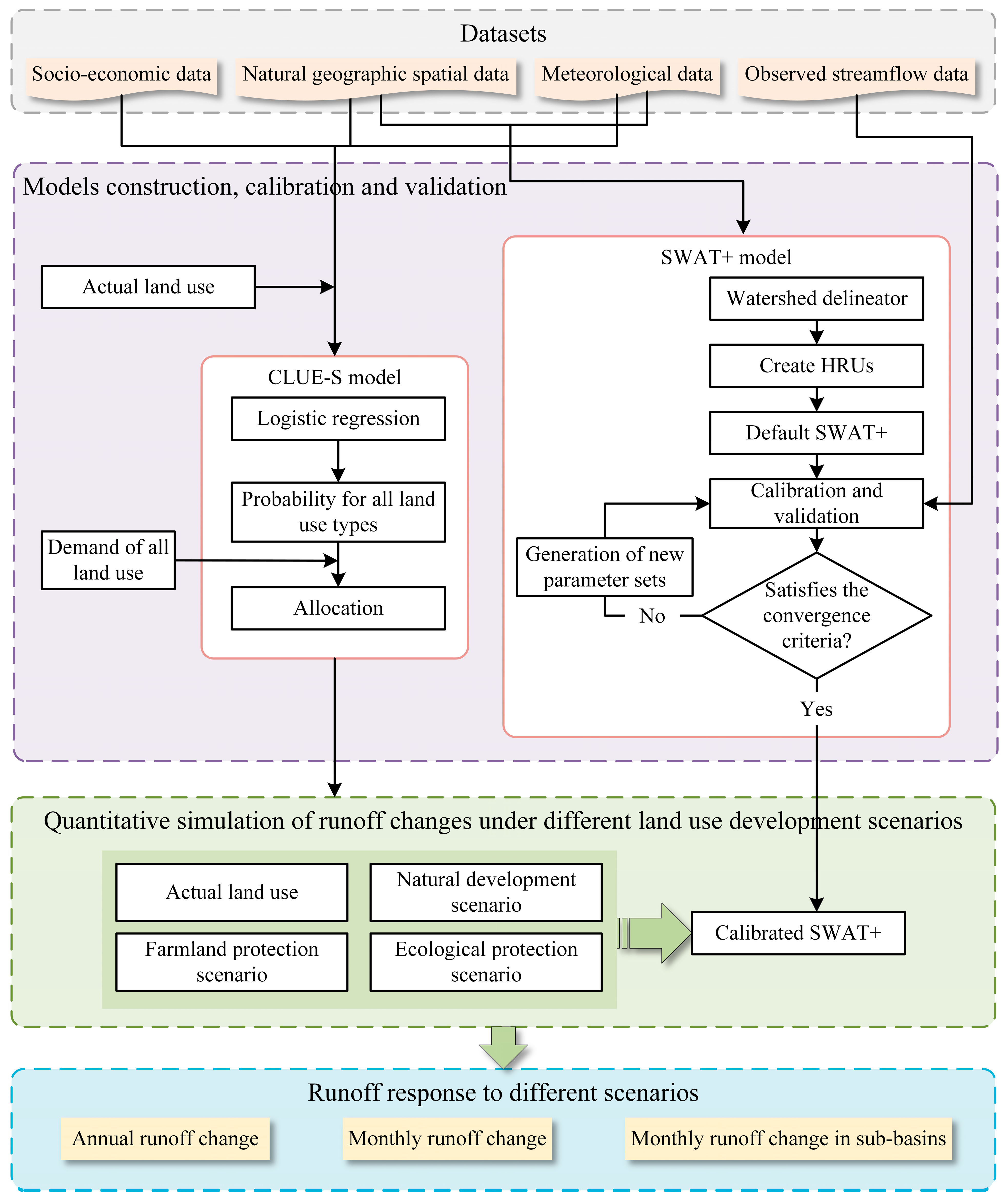
2.2. Research Framework for Runoff Response to Land Use Change

A coupling analysis framework (Figure 2) was developed in this study to analyze the changes in runoff under various land use development scenarios in the upstream mountainous area of Baiyangdian using the SWAT+ hydrological model [34] and CLUE-S land use simulation model [48]. First, a database for model simulation and verification was established. The data and their sources were thoroughly described in Section 2.3. Second, the SWAT+ hydrological model and CLUE-S land use model of the basin were established, calibrated, and verified. The CLUE-S model involved predicting the spatial distribution probabilities of various land use types by analyzing the driving factors influencing their distribution. The spatial allocation of land use demands under different scenarios was then executed through iterative processes. For the SWAT+ model, steps were followed to construct the model, the most important of which was the establishment of the Hydrological Response Units (HRUs). The HRUs were the basic computational unit of the SWAT+ model and were formed from combinations of land use types, soil types, and slope classes within different sub-basins. Detailed procedures for the construction, calibration, and validation of the SWAT+ and CLUE-S models were provided in Section 2.4 and Section 2.5. Finally, the runoff changes generated by various land use scenarios simulated by CLUE-S were quantified by the calibrated SWAT+ model. Section 2.6 provided a detailed explanation of the methods for land use scenarios setting up.

2.3. Data Source

The data used to drive both the SWAT+ and CLUE-S models primarily consist of basin spatial data, climate, and streamflow observation data. In addition, the socio-economic data are also required to drive the CLUE-S model. The nearest neighbor method was used to resample all raster data to 90 m, ensuring consistent resolution.

The Digital Elevation Model (DEM) was SRTMDEM from Geospatial Data Cloud (http://www.gscloud.cn/, accessed on 27 September 2022). The basin slope data were generated by the DEM data. The soil data were extracted from the World Soil Database (HWSD; http://fao.org/soils-portal/soil-survey, accessed on 27 September 2022). The soil characteristic parameters (soil saturated water conductivity, effective water holding capacity, and soil density) were computed by the software Soil–Plant–Atmosphere–Water [49] (SPAW). The historical land use data were acquired from the Resource and Environmental Science and Data Center (RESDC; https://www.resdc.cn, accessed on 19 October 2023). The average soil organic carbon density data of 0–5 cm, which was one of the driving factors of CLUE-S model modeling, was derived from the soil information data set SoilGrids 2.0 [50].

Historical climate data were daily observation data from three climate stations in the basin and four stations around the basin from 1959 to 2019, acquired from RESDC. In this study, a weather generator, WXGEN [51], integrated into the SWAT+ model was constructed to simulate climate data from 2020 to 2030 using the statistical characteristics of historical weather station data.

The observed data of monthly streamflow from six hydrological stations (Fuping, Zhongtangmei, Zijingguan, Zhangfang, Luobaotan, and Manshuihe) were collected from the China Hydrological Yearbook for 1969–1986.

The socio-economic data included river basin water use, river basin water withdrawal distance, population density, and GDP data, where population density and GDP were obtained from RESDC. The water withdrawal distance of the basin is the Euclidean distance between each grid and the river.

2.4. SWAT+ Model

Simulating the hydrological process in the upstream mountainous basin of Baiyangdian was achieved using SWAT+, an improved hydrological model based on SWAT. The SWAT+ uses a modular structure, allowing for greater flexibility in sub-basin discretization and configuration [34]. It also provides two options for calculating runoff, namely the Soil Conservation Service curve number (SCS-CN) procedure [52] and the Green and Ampt infiltration method [53].

Runoff simulation in this study utilized the SCS-CN method, noted for its efficiency and popularity [54,55,56]. The SCS-CN relies on an empirical formula created from extensive observations of rainfall and runoff data, incorporating various land use and other factors combinations. The specific calculation equations are as follows:

$$Q_{surf}={\displaystyle \frac{{\left(R_{day}-0.2S\right)}^2}{\left(R_{day}+0.8S\right)}}$$

(1)

where Q_surf is runoff (mm); R_day is the daily rainfall (mm); S represents the retention parameter (mm), which can be calculated by the following equation:

$$S=25.4\left({\displaystyle \frac{1000}{CN}}\right)-10$$

(2)

where CN is the curve number, typically obtained from the model user manual or determined through model parameter calibration. The CN in this study was determined by calibrating the parameter cn2.

Using the QSWAT+ plugin in QGIS, we constructed a SWAT+ model for the upstream mountainous basin of Baiyangdian, ultimately dividing it into 17 sub-basins with 3462 hydrological response units. The year range of 1966–1977 was set as the model calibration period (1966–1968 was the model warm-up period), and 1978–1980 was the model validation period in this study. Referring to existing studies [57] and sensitivity analysis using the Sobol method, 19 parameters associated with streamflow change were selected for calibration (Table S3). The detailed results of the parameter sensitivity analysis are provided in Figure S1. We utilized the multi-site calibration method [58] in this study, which employed streamflow data from multiple available hydrological stations across the entire basin for calibration. It is more effective in improving model simulation performance compared to using only the basin outlet site calibration [59,60]. Therefore, the monthly measured streamflow data from six hydrological stations were used for calibration, following the principle of upstream first and downstream later. First, the upstream hydrological stations of Fuping, Zhongtangmei, Zijingguan, and Manshuihe were calibrated. After the calibration results of the upstream stations met the accuracy requirements, the upstream parameter values were kept unchanged, and the downstream Zhangfang station was calibrated. Finally, we calibrated the Luobaotan station.

The accuracy of streamflow simulation was evaluated using three model evaluation performance indicators [41]: coefficient of determination (R²), Nash-Sutcliffe efficiency [61] (NSE), and percent bias [62] (PBIAS). The R² can be used to assess the linear correlation between the simulated and observed values, and results with R² exceeding 0.5 are generally deemed acceptable. The NSE measures the degree to which the hydrological model simulation matches the overall trend of the observed data. The PBIAS indicates the extent to which the model simulation results either overestimate or underestimate compared to the observed values. An NSE exceeded 0.7, and a PBIAS absolute value less than 25 indicates that the model performs well [63]. Following are the methods for calculating the three indicators:

$$R^2={\displaystyle \frac{{\left[\sum _{i=1}^n\left(O_i-O_{avg}\right)\left(P_i-P_{avg}\right)\right]}^2}{\sum _{i=1}^n{\left(O_i-O_{avg}\right)}^2\sum _{i=1}^n{\left(P_i-P_{avg}\right)}^2}}$$

(3)

$$\begin{array}{c}NSE=1-{\displaystyle \frac{\sum _{i=1}^n{\left(O_i-P_i\right)}^2}{\sum _{i=1}^n{\left(O_i-O_{avg}\right)}^2}}\end{array}$$

(4)

$$\begin{array}{c}PBIAS={\displaystyle \frac{\sum _{i=1}^n\left(P_i-O_i\right)}{\sum _{i=1}^n\left(O_i\right)}}\times 100\end{array}$$

(5)

where n is the number of observed data, O_i is the ith observed data, O_avg refers to the average value of the observations, P_i is the ith simulated data, and P_avg refers to the average value of the simulations.

Furthermore, model uncertainty was quantified using the 95% prediction uncertainty (95PPU) method [64]. A detailed explanation of the methodology and results can be found in the Supplementary text and Table S4.

2.5. CLUE-S Model

The land use simulation model CLUE-S [48] was employed in this study to predict future land use transformations. Assuming that in the short term, the connections among land use processes and natural and socio-economic drivers remain unchanged. The CLUE-S model simulates the spatial distributions of short-term land use change with the regression relationships between historical land use patterns and driving forces [65]. The model consists primarily of two modules: the land use demand module and the spatially explicit allocation module [66]. The spatial allocation process is accomplished using a stepwise logistic regression method, which effectively filters out driving factors that do not significantly contribute to changes in land use patterns:

$$L\mathit{og}\left({\displaystyle \frac{P_i}{1-P_i}}\right)={\beta }_0+{\beta }_1{X}_{1,i}+{\beta }_2{X}_{2,i}+\cdots +{\beta }_n{X}_{n,i}$$

(6)

where P_i is the probability that the land use type i is assigned to a certain grid cell, X_n,i is the value of driving factor n in land use type i, β₀ represents the intercept, and β_n represents the coefficient of the driving factor n in the logistic regression equation, used to indicate the correlation between the distribution probability of land use types and the driving factors.

Actual land use data from 2015 was used in this study as a simulation reference. We constructed a logistic regression model using natural climate factors (DEM, slope, soil organic carbon density, precipitation, temperature) and socio-economic factors (river water intake distance, population density, GDP) to generate the spatial suitability distribution for each land use type based on the 2015 land use pattern. The Receiver Operating Characteristic (ROC) curve was employed to assess the goodness of fit of the logistic regression model [67]. The area under the ROC curve (AUC) measures the trade-off between true and false positives across an extensive set of cut-off thresholds [68,69]. The closer the AUC result is to 1, the stronger the predictive ability and the higher the accuracy of the model.

A logistics regression model for land use, developed using the CLUE-S model, was presented in Table S5 in this study. For all land use types, AUC values exceeded 0.7, indicating a high spatial similarity between the modeled and actual land use in the established model.

To further assess CLUE-S model accuracy in predicting land use spatial distribution, we used the Kappa coefficient [70] to test the simulated land use results (Equation (7)). The Kappa coefficient spans from −1 to 1 and is deemed acceptable when above 0.7. The higher the coefficient, the more precise the simulation.

$$Kappa=\left(P_o-P_c\right)/\left(P_p-P_c\right)$$

(7)

where P_o is the correct simulation proportion; P_c is the correct simulation proportion for a random condition; P_p is the correct simulation proportion under perfect classification.

2.6. Land Use Development Scenarios Establishment

The land use demand module of the CLUE-S model is generally used in conjunction with external methods. Accordingly, this study first employed a Markov chain to predict the required quantities of different land use types across various scenarios against the backdrop of urban expansion. Subsequently, using the spatially explicit allocation module of CLUE-S and actual land use data from 2015, we simulated the spatial distribution of diverse land use development scenarios. Considering the relevant planning for future social and economic development, along with agricultural and ecological protection needs in the basin, we established three land use development scenarios:

The natural development scenario (ND): This scenario projected land use evolution to follow the 1980–2015 trend, with decreases in farmland, forest, and grassland areas and an increase in urban land areas.

The farmland protection scenario (FP): This scenario aimed to safeguard future agricultural development in the basin and mitigate potential urban land expansion in ND by reducing the probability of farmland conversion to urban areas by 50%, using conversion probabilities from 1980 to 2015.

The ecological protection scenario (EP): This scenario aimed to promote ecological restoration and curb the anticipated increase in urban land. The farmland, forest, grassland, and water were set to reduce the probability of converting into urban areas by 50%. Additionally, the forest, grassland, and water also had a 50% probability of being reduced into farmland.

3. Results

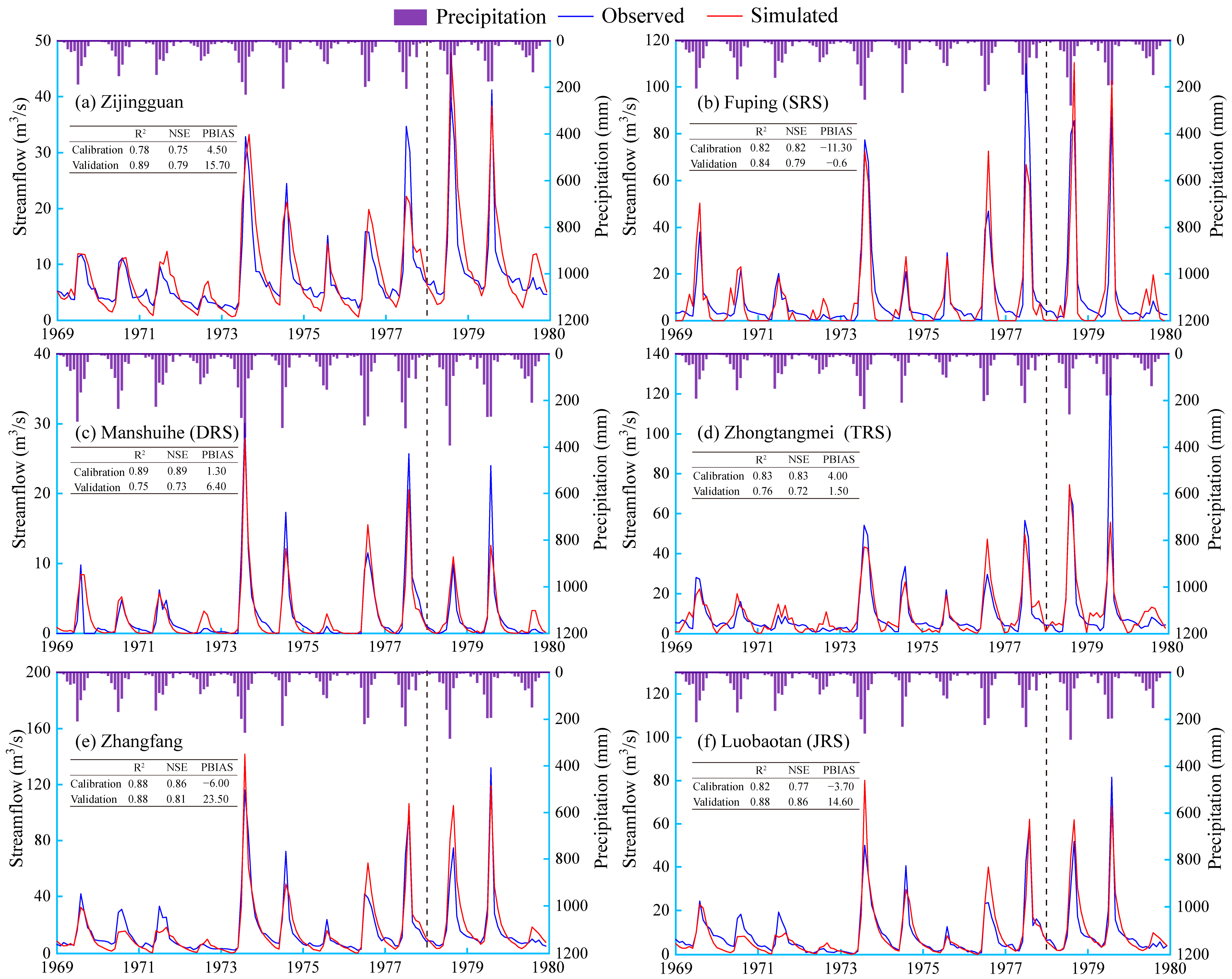
3.1. Model Calibration and Validation

Table 1. SWAT+ model parameter calibrated results (Refer to Table S3 for parameter definitions).

Parameter	Types of Change 1	Calibrated Value
		Zijingguan	Fuping	Manshuihe	Zhongtangmei	Zhangfang	Luobaotan
cn2	pctchg	5.47	−7.26	−6.12	13.60	−0.63	4.80
lat_len	abschg	−4.54	−27.79	−23.29	4.70	14.46	−8.19
lat_ttime	abschg	−0.21	5.61	25.07	−25.73	2.87	−16.56
esco	absval	0.25	0.02	0.85	0.07	0.89	0.18
epco	absval	0.34	0.35	0.69	0.57	0.06	0.75
slope	abschg	5.83	2.40	5.79	1.98	−24.37	−20.04
canmx	absval	1.94	6.36	23.10	11.68	87.06	84.20
ovn	abschg	4.87	−16.12	−24.95	−16.39	−10.26	−4.63
snofall_tmp	abschg	18.13	−8.10	17.57	26.11	−8.72	−3.42
snomelt_tmp	abschg	−3.38	3.04	7.56	−35.16	−3.50	−16.00
snomelt_max	absval	1.72	3.14	8.49	2.22	2.42	4.56
snomelt_min	absval	1.02	2.94	1.58	5.36	5.77	9.59
snomelt_lag	absval	0.13	0.17	0.97	0.64	0.34	0.43
alpha	absval	0.01	0.85	0.37	0.49	0.93	0.01
flo_min	abschg	13.37	22.53	−32.55	16.58	−21.90	−2.17
revap_co	abschg	14.26	−0.65	−31.23	25.86	25.76	8.80
revap_min	abschg	−11.60	−2.01	36.27	10.02	−11.88	19.92
k	abschg	8.19	34.85	−3.38	0.34	34.26	15.63
awc	abschg	−17.54	27.37	−7.39	−35.41	21.92	−16.74

¹ Note: pctchg refers to change the value by the specified percent; abschg refers to change the value by the specified amount; absval refers to change the value of the parameter.

displays the parameter calibration results from 1966 to 1977. The calibrated model performed well during the validation period, with simulated and observed streamflow changes showing consistent trends (Figure 3). Throughout the entire simulation period, the simulated streamflow during the non-flood season indicated lower simulation accuracy for low streamflow compared to high streamflow. This discrepancy might be attributed to inadequate modeling of groundwater changes in the region by the groundwater simulation module of the SWAT+ model [71]. Figure 3 also presents the simulation accuracy for each hydrological station. All these stations achieved NSE values exceeding 0.70, with R² values above 0.75, indicating satisfactory simulation accuracy and validating the reliability of the model results.

The constructed CLUE-S model was used to simulate the land use distribution for 2015. A Kappa coefficient of 0.83 (

Table 2. Comparison of simulation and observation results of land use patterns in 2015.

Kappa = 0.83		Number of Simulated Grids
		Farmland	Forest	Grassland	Water	Urban	Bare Land	Producer Accuracy%
Number of actual grids	Farmland	136,140	5170	14,068	2514	4739	16	83.70
	Forest	5428	635,004	33,398	1030	2216	13	93.78
	Grassland	14,276	32,878	442,689	1556	7335	32	88.76
	Water	1904	1236	1819	11,523	558	1	67.62
	Urban	4880	2787	6755	373	14,849	55	50.00
	Bare land	0	14	36	66	0	0	0.00
	User accuracy%	83.71	93.78	88.76	67.54	50.00	0.00	-

) was obtained, demonstrating a high level of consistency comparing the simulated land use with the actual land use in 2015. The overall accuracy of the land use simulation was considered acceptable, supporting the model application in future land use scenario simulations.

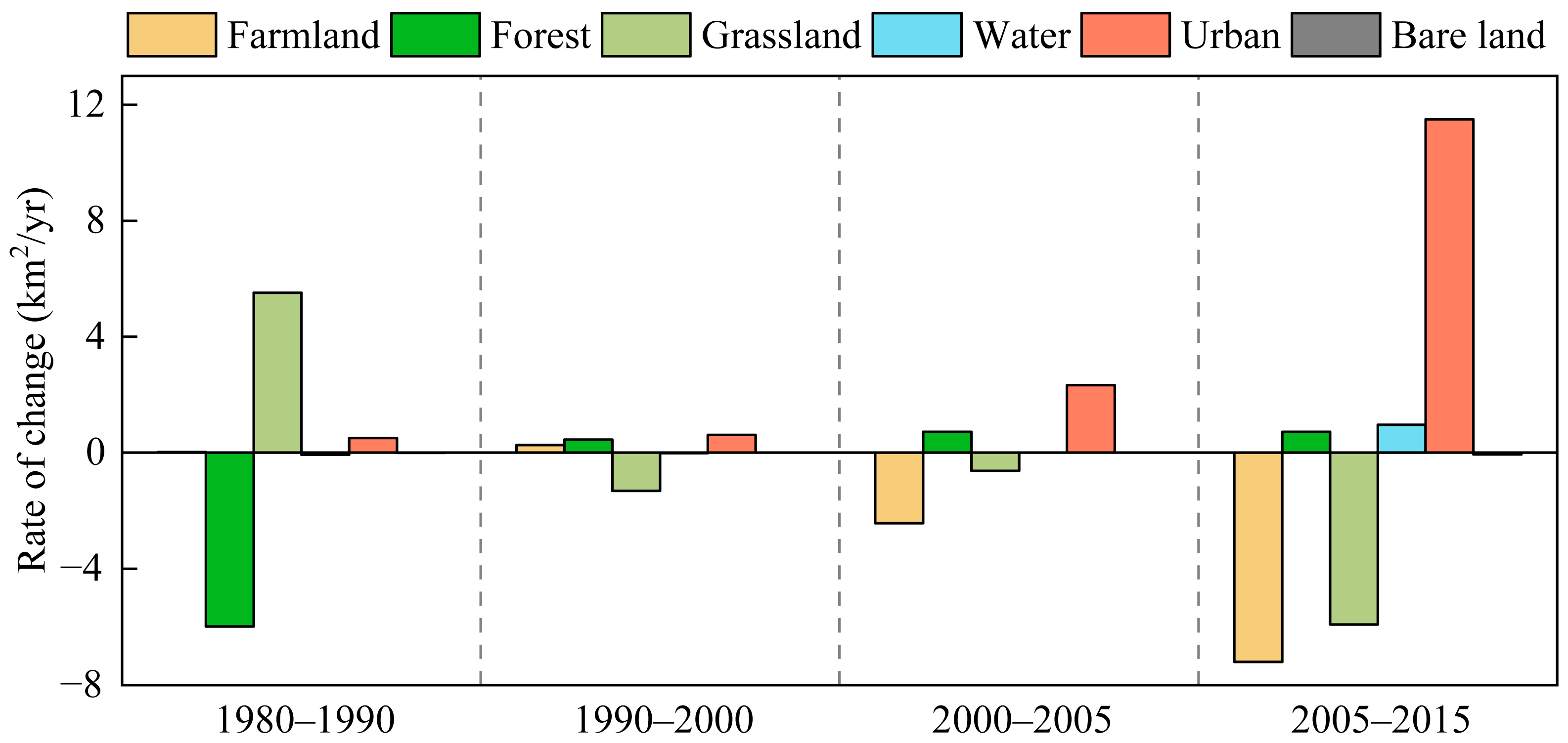
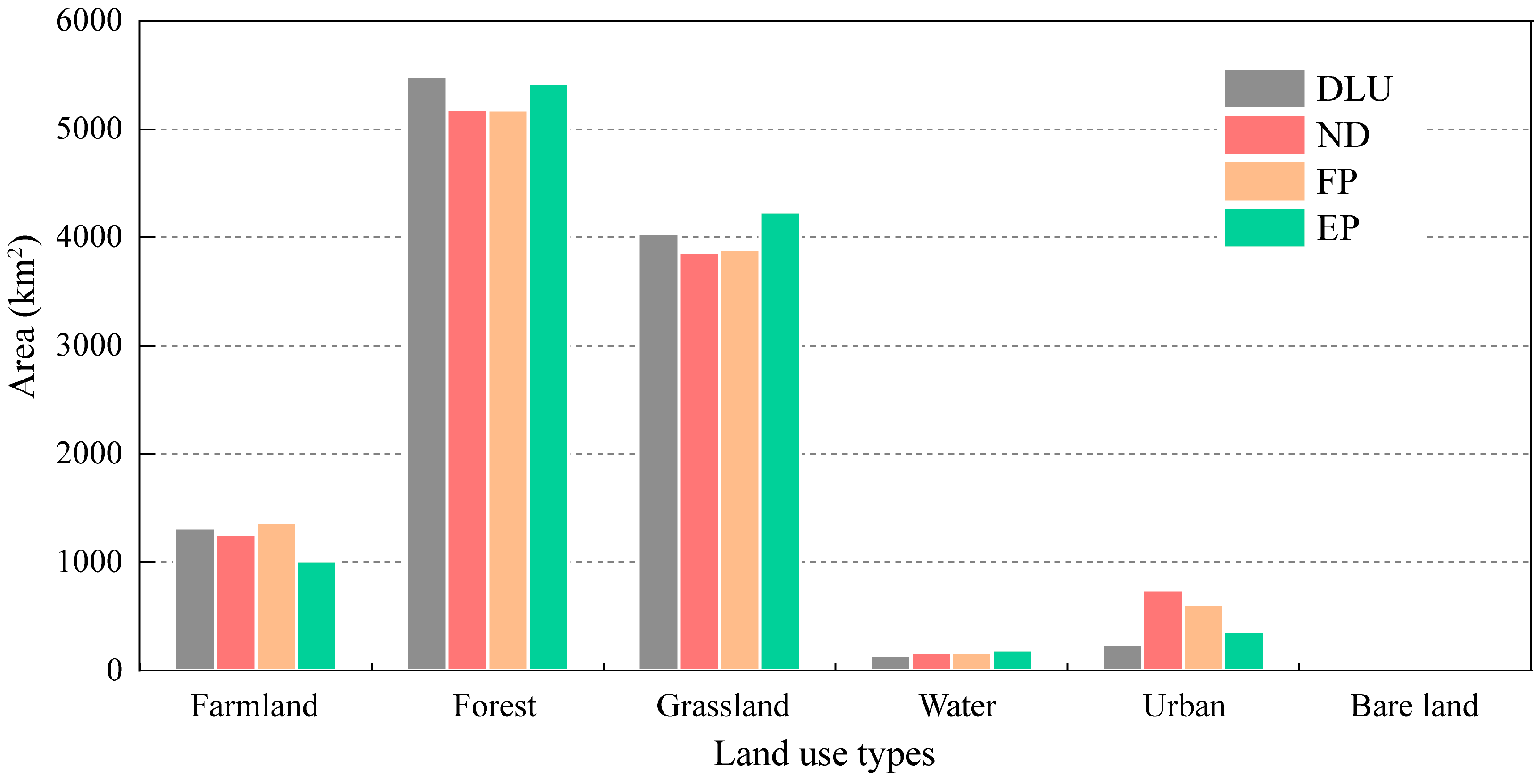
3.2. Historical Land Use Changes and Land Use Development Scenarios

The land use changes in the upstream mountainous basin of Baiyangdian displayed various characteristics in different periods (Figure 4). During the decade from 1980 to 1990, the forest in the watershed decreased rapidly (−5.98 km²/year), while the grassland increased significantly (5.52 km²/year). From 1990 to 2000, grassland areas began to decline, with other land use types increasing. Between 2000 and 2005, farmland decreased. From 2005 to 2015, farmland and grassland areas decreased sharply at rates of 7.20 km²/year and 5.91 km²/year, respectively, alongside an accelerated urban expansion rate of 11.50 km²/year. In summary, socio-economic development in the basin from 1980 to 2015 had led to an increasingly dominant annual rate of urban expansion. According to the land use transition matrix for this period (

Table 3. Land use transfer matrix in the upstream mountainous area of Baiyangdian from 1980 to 2015 (km²).

1980	2015
	Farmland	Forest	Grassland	Water	Urban	Bare Land	Transfer-Out Area
Farmland	1138.21	52.21	124.89	16.94	66.52	0.00	260.55
Forest	42.62	5175.68	271.85	10.59	27.97	0.11	353.14
Grassland	111.29	245.61	3628.92	14.45	59.69	0.23	431.28
Water	15.23	5.04	10.61	95.09	3.22	0.00	34.10
Urban	10.07	4.96	3.62	0.97	83.16	0.00	19.62
Bare land	0.02	0.92	0.11	0.00	0.00	0.60	1.05
Transfer-in area	179.23	308.74	411.08	42.95	157.40	0.34	1099.74
Net increase	−81.32	−44.40	−20.19	8.85	137.78	−0.71	-

), urban land saw the most significant increase (137.78 km²), while farmland experienced the largest decrease (81.32 km²). The expanded urban construction land primarily originated from farmland and grassland.

Land use changes from 1980 to 2015 differed among the various sub-watersheds, but all showed an increase in urban construction land (Figure 5). In SRS, the primary changes included the reduction of grassland and the increase of both forest and urban land. The predominant change in TRS was the growth of urban land. The JRS experienced the most extensive land use changes, marked by a 69.00 km² increase in urban land and reductions of 64.21 km² in farmland and 43.69 km² in forest. Despite the less dramatic land use changes in DRS, urban land continued to expand.

Figure 6 illustrates the projected land use areas in 2030 for three different development scenarios derived from the default land use (DLU) simulation of 2015. In scenario ND, a significant urban expansion at a rate of 33.65 km²/year dominated the land use change compared to DLU. By 2030, the urban area was anticipated to increase by 209.85%. In addition, farmland (−4.38%), forest (−5.45%), and grassland (−4.43%) all experienced reductions. In the scenario FP, the urban area expansion rate decreased to 24.65 km²/year. The final urban area increased by 153.69%, and the farmland increased by 3.66%. For the scenario EP, urban area expansion was the slowest at 8.28 km²/year, leading to a final increase of 51.64%. The grassland and water areas rose by 4.80% and 37.23%, respectively. Although the forest area was slightly lower than in DLU, it increased significantly compared to FP and EP scenarios. Generally, urban expansion remained the main trend for future development despite varying degrees of restrictions on the urban growth rate in the FP and EP scenarios.

Under varying land use scenarios, the dominant land use types in the four sub-basins remained unchanged, but the area ratios differed (Figure 7). The SRS sub-basin was predominantly covered by grassland (54.92–57.56%) and forest (37.41–38.36%). In the TRS and JRS, extensive areas of grassland (TRS: 49.38–53.88%; JRS: 19.19–21.81%), forest (TRS: 23.23–25.30%; JRS: 62.85–65.03%) and farmland (TRS: 16.18–20.63%; JRS: 7.99–11.20%) were noted. In the DRS, forest (67.56–76.58%) and urban areas (13.23–27.10%) were the primary land use types, with their proportions changing significantly.

3.3. The Impact of Historical Land Use on Runoff

Examining annual variation trends in simulated runoff differences under historical land use conditions in 1980 and 2015 provided insights into the hydrological responses of the upstream mountainous basin of Baiyangdian and its sub-basins. From 1969 to 2018, the differences in runoff simulated with 2015 land use versus 1980 land use were consistently positive, ranging mainly from 0.5 to 1.3 mm, except in 1996 (Figure 8). The observed land use changes by 2015, characterized by urban expansion and reductions in farmland, forest, and grassland areas, resulted in increased runoff.

From the sub-watershed perspective, runoff changes predominantly increased in three sub-watersheds except for the SRS. The TRS experienced the most significant increase. Influenced by the 2015 land use changes, the runoff in the SRS decreased by an average of 0.3 mm. The TRS exhibited the highest increase in runoff, averaging 1.7 mm. Runoff in DRS and JRS raised by 0.8 mm and 0.7 mm, respectively, similar to the overall basin trend.

3.4. Runoff Response to Different Land Use Change Scenarios

Simulation of runoff changes in the upstream mountainous basin of Baiyangdian under three land use development scenarios from 2020 to 2030 was conducted using the calibrated SWAT+ model. The trends in average annual total runoff changes were not significant across the scenarios, though all showed an increase (Figure 9a). Compared to the DLU, the average annual total runoff increased the most in the FP scenario (10.9%), followed by the ND (8.9%) and EP (7.7%) scenarios. Monthly total runoff changes showed the most pronounced differences from July to August (Figure 9b), with the ND scenario showing the highest runoff totals. The scenario EP had the greatest effect on reducing the runoff peak compared to the ND and FP scenarios.

Figure 10 presents the monthly total runoff of the four major sub-basins in the upstream mountainous area of Baiyangdian and its monthly changes compared to the DLU under different scenarios. Runoff changes in each sub-basin exhibited distinct seasonal differentiation across the three land use development scenarios. During the summer flood season (May to October), runoff in each basin increased substantially with rising precipitation. From November to April, the runoff remained relatively low in SRS and DRS, while TRS and JRS experienced significant changes. Monthly runoff changes exhibited noticeable scenario variability across all sub-basins under different land use development scenarios. Scenario differences in monthly runoff in SRS were most pronounced from September to December compared to the remaining months. The runoff in TRS was highest and increased the most in EP from March to April and October to November, while it was the lowest in ND. Additionally, the rate of runoff increase from June to August in EP was significantly lower than in ND and FP. The disparity in runoff changes across various scenarios in the JRS was most apparent from May to August. Runoff variations displayed an upward trend relative to the DLU scenario, with EP showing the least amount of increase. In the DRS, the most significant runoff changes occurred from May to August under different land use development scenarios, with runoff notably lower in EP compared to ND and FP.

Figure 11 presents the monthly water yield for each land use type, aiming to explore the impact of land use changes on basin runoff more thoroughly. Substantial disparities in water yield were observed across different land use types. However, for each land use type, the alterations in water yield were remarkably alike across different scenarios. Urban land exhibited the highest annual water yield values, notably from June to September, contributing the most to overall water yield. Grassland, farmland, bare land, and forest exhibited similar patterns in water yield, peaking in August. Grassland had the highest water yield, while forest had the lowest. Minimal water yield was observed for all land use types during the dry months (November to April). In terms of annual variation in water yield, urban land demonstrated the most significant changes over the year, whereas forest maintained consistently low levels.

4. Discussion

4.1. Impacts of Different Land Use Scenarios on Runoff

Numerous studies have demonstrated that shifts in spatial patterns of land use can influence the basin runoff [41,72,73,74,75,76]. Historical land use changes from 1980 to 2015 in the upstream mountainous region of Baiyangdian showed increased urban construction land and decreased farmland and grassland areas (Figure 4). According to Han et al. [77], a notable increase in construction land has occurred in the Baiyangdian Basin since the start of the 21st century. This increase indicated that land use changes in the upstream mountainous area of Baiyangdian were consistent with trends observed throughout the entire basin, reflecting the broader impact of socio-economic development. These land use changes resulted in a runoff increase for the whole basin, although the impact was not significant (Figure 8). Lyu et al. [8] found that urban expansion significantly increased runoff in the Fenhe Basin. This result indicated that the effect of urbanization on runoff varies with different basin characteristics. Additionally, runoff in the SRS generally decreased, while runoff in other sub-basins increased (Figure 8). Grassland loss and forest rise might be contributing to the runoff decrease in SRS (Figure 5), a pattern consistent with findings by Xu et al. [78], who reported similar vegetation shifts leading to reduced runoff in forested sub-basins. Additionally, the expansion of urban land in SRS might partially offset the reduction in runoff.

This study further established various land use development scenarios based on historical urbanization trends. The monthly runoff changes in these scenarios closely matched the precipitation distribution, highlighting precipitation as the main factor influencing runoff variations in the basin [79,80,81,82,83]. In this study, the impacts of climate change under different scenarios were controlled using the same meteorological data. Therefore, the discrepancies in runoff changes across different scenarios only came from the different land use spatial patterns. At both annual and monthly scales, the scenario EP yielded the lowest runoff, whereas FP generated the highest (Figure 9). In the scenario EP, the substantial increase in forest resulted in a slowdown in surface flow velocity and an increase in surface soil organic matter, which ultimately increased precipitation infiltration and reduced surface runoff [84,85,86,87]. At the same time, the runoff peaks were attenuated due to the retention of precipitation by the forest canopy, surface litter layer, and enhanced soil infiltration, while water sources conserved by the forest were able to recharge runoff during the dry season [88,89,90,91,92,93]. This could be reflected in the findings of this study (Figure 9 and Figure 10). In the scenario FP, due to repeated cultivation of farmland, simple vegetation, and low coverage, it was easily affected by soil erosion [75,94]. Consequently, the farmland increase could result in higher runoff. Additionally, urban development reduced vegetation cover and increased impermeable surfaces, which decreased soil infiltration and water storage capacity, further increasing surface runoff [95,96,97]. Meanwhile, according to the changes in water yield by land use type (Figure 11), it could be predicted that the larger the urban expansion in the upstream mountainous basin of Baiyangdian, the larger the runoff, especially from June to September, with abundant precipitation. Consequently, the ND scenario exhibited the highest monthly runoff peaks.

4.2. Implications and Policies for Different Sub-Basins

The differences among the four main sub-watersheds in the upstream mountainous area of Baiyangdian under various land use development scenarios might stem from the varying proportions of land use types in each scenario. Among these, DRS exhibited notable differences in monthly runoff changes compared to the other sub-basins (Figure 10). Forest comprised more than 65% of DRS. Under the scenario EP, forest increase was greater than in other sub-basins (Figure 7). Consequently, its role in regulating peak runoff was the most significant. Additionally, precipitation differences across sub-basins also affected runoff production. In sub-basins with abundant precipitation, such as DRS and JRS (Figure 3), urban expansion was expected to positively influence runoff increases (Figure 11), but the potential threat of flooding should be considered. Therefore, these factors exerted a complex influence on sub-basin runoff responses. To address the challenges posed by the complex impact of urbanization-driven land use changes on runoff, implementing targeted management strategies is crucial. For forested sub-basins like DRS, priority should be given to preserving and expanding forest cover to sustain its runoff-regulating benefits [98]. In contrast, for areas such as JRS, which are experiencing urban expansion and increased runoff, flood mitigation measures should be emphasized [99]. These include enhancing drainage infrastructure, incorporating permeable surfaces, and applying sustainable urban planning practices [95,100]. By tailoring countermeasures to the specific characteristics and challenges of each sub-basin, these strategies will not only protect water resources to ensure downstream water supply but also promote sustainable land use practices and enhance overall watershed resilience.

4.3. Limitations and Uncertainties

Distributed hydrological models possess certain uncertainties resulting from their multi-parameter nature, varied input data, and the model complexities construction process [101,102,103]. With only seven climate stations available in this study and their uneven distribution, this is also a source of errors between simulated and measured streamflow [104,105]. The varying topography, land use types, and soil types of each sub-basin also increase the model uncertainty [60,106]. Therefore, to reduce model uncertainty, a multi-site calibration method was employed during the calibration period, which ultimately achieved good simulation performance (Figure 3). In simulating land use spatial distribution, the limited number and quality of driving factors chosen for the CLUE-S introduced a certain degree of uncertainty into the constructed model. Additionally, the Markov chain was employed to forecast future land use demand, which, to some extent, ignored the systematic and stochastic nature of future land use changes [107].

Although climate and land use change are closely related [108,109,110], this study did not consider their interaction effect when analyzing the impact of land use on runoff change. The long-term changes in land use are influenced by climate change through its effects on natural vegetation growth and human activities, including water use [111,112,113,114]. Meanwhile, land use changes can influence local temperature fluctuations by modifying the surface albedo [115,116,117]. Changes in land use type also impact greenhouse gas emissions, therefore affecting climate change [118,119]. Therefore, a complex and changeable relationship exists between climate and land use. Accordingly, future research should consider their interaction more comprehensively.

5. Conclusions

By integrating the SWAT+ with the CLUE-S, this study examined runoff changes in the upstream mountainous area of Baiyangdian across three land use evolution scenarios within an urbanization context. The primary research findings are summarized as follows:

(1)

In the upstream mountainous basin of Baiyangdian, SWAT+ was well applicable, with NSE values exceeding 0.7 for all hydrological stations. The simulated land use data generated by the CLUE-S model demonstrated high spatial distribution consistency with real data, achieving a Kappa coefficient of 0.83.

(2)

Urban land expansion drove changes in land use in ND, FP, and EP, while the FP and EP decelerated this expansion. Additionally, the scenario EP effectively controlled the reduction of forest area in the basin.

(3)

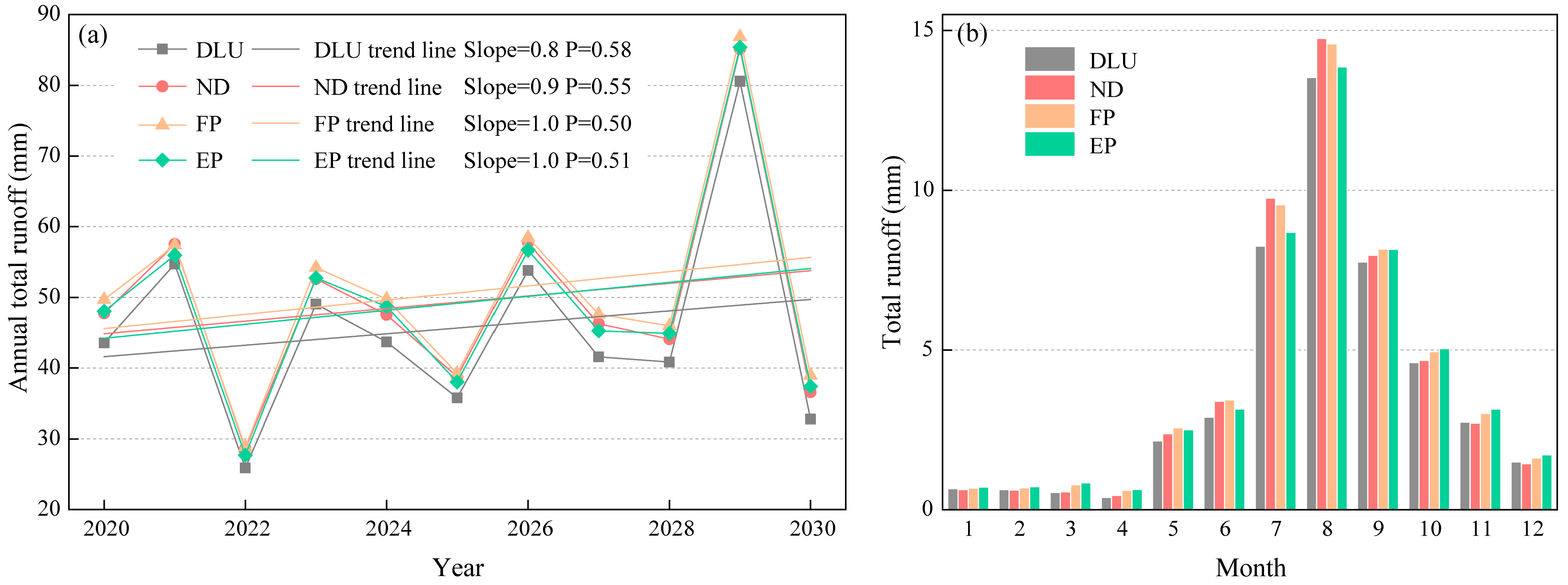
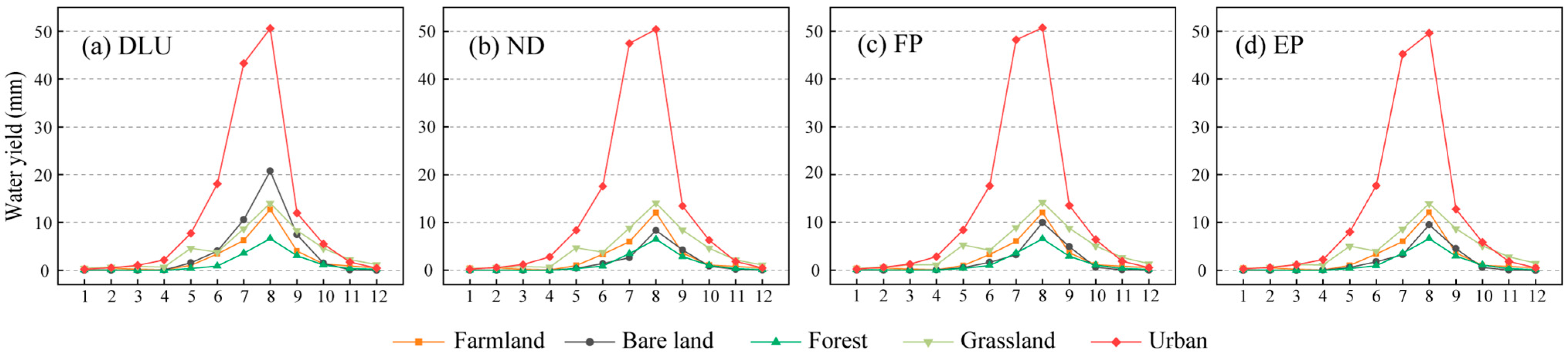
The annual runoff in the upstream basin of Baiyangdian showed an upward trend under the influence of historical urbanization trends in land use. The simulated annual runoff changes under different land use scenarios also exhibited an upward trend, with no significant differences observed among the three scenarios. However, significant seasonal disparities in runoff changes were observed under different scenarios. Generally, the ND and FP scenarios promoted runoff production from May to October, while the EP scenario had a significant reduction effect on the monthly runoff peak from July to August, particularly in the DRS. These differences were mainly attributed to the different contributions of various land use types to water yield.

These findings support local water resource management in the upstream mountainous area of Baiyangdian and provide a scientific basis for future water supply decisions. Beyond this region, the study offers valuable insights applicable to similar watershed challenges globally, especially in areas undergoing rapid urbanization. The methodologies and conclusions can inform ecological security and sustainable development strategies, including in Xiong’an New Area. Additionally, this study contributed to the field of hydrology by demonstrating the importance of integrating multiple land use scenarios in runoff modeling, particularly in the context of urbanization.

References

1. Song, X.-P.; Hansen, M.C.; Stehman, S.V.; Potapov, P.V.; Tyukavina, A.; Vermote, E.F.; Townshend, J.R. Global land change from 1982 to 2016. Nature 2018, 560, 639–643. [Google Scholar] [CrossRef]
2. Sun, L.; Chen, J.; Li, Q.; Huang, D. Dramatic uneven urbanization of large cities throughout the world in recent decades. Nat. Commun. 2020, 11, 5366. [Google Scholar] [CrossRef] [PubMed]
3. Foley, J.A.; DeFries, R.; Asner, G.P.; Barford, C.; Bonan, G.; Carpenter, S.R.; Chapin, F.S.; Coe, M.T.; Daily, G.C.; Gibbs, H.K.; et al. Global Consequences of Land Use. Science 2005, 309, 570–574. [Google Scholar] [CrossRef] [PubMed]
4. Chen, H.; Huang, J.J.; Dash, S.S.; McBean, E.; Wei, Y.; Li, H. Assessing the impact of urbanization on urban evapotranspiration and its components using a novel four-source energy balance model. Agric. For. Meteorol. 2022, 316, 108853. [Google Scholar] [CrossRef]
5. Stephens, C.M.; Lall, U.; Johnson, F.M.; Marshall, L.A. Landscape changes and their hydrologic effects: Interactions and feedbacks across scales. Earth Sci. Rev. 2021, 212, 103466. [Google Scholar] [CrossRef]
6. Wagner, P.D.; Kumar, S.; Fohrer, N. Integrated modeling of global change impacts on land and water resources. Sci. Total Environ. 2023, 892, 164673. [Google Scholar] [CrossRef]
7. Zhang, Y.; He, Y.; Song, J. Effects of climate change and land use on runoff in the Huangfuchuan Basin, China. J. Hydrol. 2023, 626, 130195. [Google Scholar] [CrossRef]
8. Lyu, X.; Jia, Y.; Qiu, Y.; Du, J.; Hao, C.; Dong, H.; Chang, J. Influence of human-induced land use change on hydrological processes in semi-humid and semi-arid region: A case in the Fenhe River Basin. J. Hydrol. Reg. Stud. 2024, 51, 101605. [Google Scholar] [CrossRef]
9. Mahtta, R.; Fragkias, M.; Güneralp, B.; Mahendra, A.; Reba, M.; Wentz, E.A.; Seto, K.C. Urban land expansion: The role of population and economic growth for 300+ cities. NPJ Urban Sustain. 2022, 2, 5. [Google Scholar] [CrossRef]
10. Gao, J.; O’Neill, B.C. Mapping global urban land for the 21st century with data-driven simulations and Shared Socioeconomic Pathways. Nat. Commun. 2020, 11, 2302. [Google Scholar] [CrossRef]
11. Li, C.; Sun, G.; Caldwell, P.V.; Cohen, E.; Fang, Y.; Zhang, Y.; Oudin, L.; Sanchez, G.M.; Meentemeyer, R.K. Impacts of Urbanization on Watershed Water Balances Across the Conterminous United States. Water Resour. Res. 2020, 56, e2019WR026574. [Google Scholar] [CrossRef]
12. Mahmoud, S.H.; Gan, T.Y. Urbanization and climate change implications in flood risk management: Developing an efficient decision support system for flood susceptibility mapping. Sci. Total Environ. 2018, 636, 152–167. [Google Scholar] [CrossRef]
13. Wilson, T.S.; Sleeter, B.M.; Cameron, D.R. Future land-use related water demand in California. Environ. Res. Lett. 2016, 11, 054018. [Google Scholar] [CrossRef]
14. Liu, X.; Liu, Y.; Wang, Y.; Liu, Z. Evaluating potential impacts of land use changes on water supply–demand under multiple development scenarios in dryland region. J. Hydrol. 2022, 610, 127811. [Google Scholar] [CrossRef]
15. Yang, D.; Luan, W.-X.; Zhang, X. Projecting spatial interactions between global population and land use changes in the 21st century. NPJ Urban Sustain. 2023, 3, 53. [Google Scholar] [CrossRef]
16. Ning, J.; Liu, J.; Kuang, W.; Xu, X.; Zhang, S.; Yan, C.; Li, R.; Wu, S.; Hu, Y.; Du, G.; et al. Spatiotemporal patterns and characteristics of land-use change in China during 2010–2015. J. Geogr. Sci. 2018, 28, 547–562. [Google Scholar] [CrossRef]
17. Ali, S.; Sethy, B.K.; Singh, R.K.; Parandiyal, A.K.; Kumar, A. Quantification of Hydrologic Response of Staggered Contour Trenching for Horti-pastoral Land Use System in Small Ravine Watersheds: A Paired Watershed Approach. Land Degrad. Dev. 2017, 28, 1237–1252. [Google Scholar] [CrossRef]
18. Aghsaei, H.; Mobarghaee Dinan, N.; Moridi, A.; Asadolahi, Z.; Delavar, M.; Fohrer, N.; Wagner, P.D. Effects of dynamic land use/land cover change on water resources and sediment yield in the Anzali wetland catchment, Gilan, Iran. Sci. Total Environ. 2020, 712, 136449. [Google Scholar] [CrossRef]
19. Sabitha, N.M.; Thampi, S.G.; Kumar, D.S. Application of a Distributed Hydrologic Model to Assess the Impact of Climate and Land-use Change on Surface Runoff from a Small Urbanizing Watershed. Water Resour. Manag. 2023, 37, 2347–2368. [Google Scholar] [CrossRef]
20. Wei, X.; Liu, W.; Zhou, P. Quantifying the Relative Contributions of Forest Change and Climatic Variability to Hydrology in Large Watersheds: A Critical Review of Research Methods. Water 2013, 5, 728–746. [Google Scholar] [CrossRef]
21. Li, Z.; Liu, W.-Z.; Zhang, X.-C.; Zheng, F.-L. Impacts of land use change and climate variability on hydrology in an agricultural catchment on the Loess Plateau of China. J. Hydrol. 2009, 377, 35–42. [Google Scholar] [CrossRef]
22. Nie, N.; Zhang, W.; Liu, M.; Chen, H.; Zhao, D. Separating the impacts of climate variability, land-use change and large reservoir operations on streamflow in the Yangtze River basin, China, using a hydrological modeling approach. Int. J. Digital Earth 2021, 14, 231–249. [Google Scholar] [CrossRef]
23. Guo, W.; Yu, L.; Huang, L.; He, N.; Chen, W.; Hong, F.; Wang, B.; Wang, H. Ecohydrological response to multi-model land use change at watershed scale. J. Hydrol. Reg. Stud. 2023, 49, 101517. [Google Scholar] [CrossRef]
24. Wu, S.; Tetzlaff, D.; Yang, X.; Soulsby, C. Disentangling the Influence of Landscape Characteristics, Hydroclimatic Variability and Land Management on Surface Water NO3-N Dynamics: Spatially Distributed Modeling Over 30 yr in a Lowland Mixed Land Use Catchment. Water Resour. Res. 2022, 58, e2021WR030566. [Google Scholar] [CrossRef]
25. Ali, M.; Khan, S.J.; Aslam, I.; Khan, Z. Simulation of the impacts of land-use change on surface runoff of Lai Nullah Basin in Islamabad, Pakistan. Landsc. Urban Plann. 2011, 102, 271–279. [Google Scholar] [CrossRef]
26. Zhou, F.; Xu, Y.; Chen, Y.; Xu, C.Y.; Gao, Y.; Du, J. Hydrological response to urbanization at different spatio-temporal scales simulated by coupling of CLUE-S and the SWAT model in the Yangtze River Delta region. J. Hydrol. 2013, 485, 113–125. [Google Scholar] [CrossRef]
27. Ji, G.; Lai, Z.; Xia, H.; Liu, H.; Wang, Z. Future Runoff Variation and Flood Disaster Prediction of the Yellow River Basin Based on CA-Markov and SWAT. Land 2021, 10, 421. [Google Scholar] [CrossRef]
28. Lyu, Y.; Chen, H.; Cheng, Z.; He, Y.; Zheng, X. Identifying the impacts of land use landscape pattern and climate changes on streamflow from past to future. J. Environ. Manag. 2023, 345, 118910. [Google Scholar] [CrossRef]
29. Singh, V.; Karan, S.K.; Singh, C.; Samadder, S.R. Assessment of the capability of SWAT model to predict surface runoff in open cast coal mining areas. Environ. Sci. Pollut. Res. 2023, 30, 40073–40083. [Google Scholar] [CrossRef] [PubMed]
30. Le, X.; Kim, Y.; Van Binh, D.; Jung, S.; Hai Nguyen, D.; Lee, G. Improving rainfall-runoff modeling in the Mekong river basin using bias-corrected satellite precipitation products by convolutional neural networks. J. Hydrol. 2024, 630, 130762. [Google Scholar] [CrossRef]
31. Zhang, P.; Cai, Y.; He, Y.; Xie, Y.; Zhang, X.; Li, Z. Changes of vegetational cover and the induced impacts on hydrological processes under climate change for a high-diversity watershed of south China. J. Environ. Manag. 2022, 322, 115963. [Google Scholar] [CrossRef] [PubMed]
32. Aznarez, C.; Jimeno-Sáez, P.; López-Ballesteros, A.; Pacheco, J.P.; Senent-Aparicio, J. Analysing the Impact of Climate Change on Hydrological Ecosystem Services in Laguna del Sauce (Uruguay) Using the SWAT Model and Remote Sensing Data. Remote Sens. 2021, 13, 2014. [Google Scholar] [CrossRef]
33. Lin, B.; Chen, X.; Yao, H.; Chen, Y.; Liu, M.; Gao, L.; James, A. Analyses of landuse change impacts on catchment runoff using different time indicators based on SWAT model. Ecol. Indic. 2015, 58, 55–63. [Google Scholar] [CrossRef]
34. Bieger, K.; Arnold, J.G.; Rathjens, H.; White, M.J.; Bosch, D.D.; Allen, P.M.; Volk, M.; Srinivasan, R. Introduction to SWAT+, A Completely Restructured Version of the Soil and Water Assessment Tool. J. Am. Water Resour. Assoc. 2017, 53, 115–130. [Google Scholar] [CrossRef]
35. Gassman, P.W.; Reyes, M.R.; Green, C.H.; Arnold, J.G. The soil and water assessment tool: Historical development, applications, and future research directions. Trans. ASABE 2007, 50, 1211–1250. [Google Scholar] [CrossRef]
36. Wagner, P.D.; Bieger, K.; Arnold, J.G.; Fohrer, N. Representation of hydrological processes in a rural lowland catchment in Northern Germany using SWAT and SWAT+. Hydrol. Processes 2022, 36, e14589. [Google Scholar] [CrossRef]
37. Jiménez-Navarro, I.C.; Jimeno-Sáez, P.; López-Ballesteros, A.; Pérez-Sánchez, J.; Senent-Aparicio, J. Impact of Climate Change on the Hydrology of the Forested Watershed That Drains to Lake Erken in Sweden: An Analysis Using SWAT+ and CMIP6 Scenarios. Forests 2021, 12, 1803. [Google Scholar] [CrossRef]
38. Wallington, K.; Cai, X. Updating SWAT+ to Clarify Understanding of In-Stream Phosphorus Retention and Remobilization: SWAT+P.R&R. Water Resour. Res. 2023, 59, e2022WR033283. [Google Scholar] [CrossRef]
39. Mohammadi Igder, O.; Alizadeh, H.; Mojaradi, B.; Bayat, M. Multivariate assimilation of satellite-based leaf area index and ground-based river streamflow for hydrological modelling of irrigated watersheds using SWAT+. J. Hydrol. 2022, 610, 128012. [Google Scholar] [CrossRef]
40. Yimer, E.A.; Riakhi, F.-E.; Bailey, R.T.; Nossent, J.; van Griensven, A. The impact of extensive agricultural water drainage on the hydrology of the Kleine Nete watershed, Belgium. Sci. Total Environ. 2023, 885, 163903. [Google Scholar] [CrossRef]
41. Xiao, F.; Wang, X.; Fu, C. Impacts of land use/land cover and climate change on hydrological cycle in the Xiaoxingkai Lake Basin. J. Hydrol. Reg. Stud. 2023, 47, 101422. [Google Scholar] [CrossRef]
42. Chawanda, C.J.; Arnold, J.; Thiery, W.; van Griensven, A. Mass balance calibration and reservoir representations for large-scale hydrological impact studies using SWAT+. Clim. Chang. 2020, 163, 1307–1327. [Google Scholar] [CrossRef]
43. Yang, Y.; Yang, X.; Li, E.; Huang, W. Transitions in land use and cover and their dynamic mechanisms in the Haihe River Basin, China. Environ. Earth Sci. 2021, 80, 50. [Google Scholar] [CrossRef]
44. Yang, L.; Zhao, G.; Tian, P.; Mu, X.; Tian, X.; Feng, J.; Bai, Y. Runoff changes in the major river basins of China and their responses to potential driving forces. J. Hydrol. 2022, 607, 127536. [Google Scholar] [CrossRef]
45. Cui, B.; Li, X.; Zhang, K. Classification of hydrological conditions to assess water allocation schemes for Lake Baiyangdian in North China. J. Hydrol. 2010, 385, 247–256. [Google Scholar] [CrossRef]
46. Hu, S.; Wang, X.; Song, X. Could the hydrological conditions of Lake Baiyangdian support a booming metropolis? Sci. Total Environ. 2023, 869, 161764. [Google Scholar] [CrossRef] [PubMed]
47. Yang, W.; Yang, Z. Development of a Long-term, Ecologically Oriented Dam Release Plan for the Lake Baiyangdian Sub-basin, Northern China. Water Resour. Manag. 2013, 27, 485–506. [Google Scholar] [CrossRef]
48. Verburg, P.H.; Soepboer, W.; Veldkamp, A.; Limpiada, R.; Espaldon, V.; Mastura, S.S.A. Modeling the Spatial Dynamics of Regional Land Use: The CLUE-S Model. Environ. Manag. 2002, 30, 391–405. [Google Scholar] [CrossRef]
49. Saxton, K.E.; Rawls, W.J. Soil Water Characteristic Estimates by Texture and Organic Matter for Hydrologic Solutions. Soil Sci. Soc. Am. J. 2006, 70, 1569–1578. [Google Scholar] [CrossRef]
50. Poggio, L.; de Sousa, L.M.; Batjes, N.H.; Heuvelink, G.B.M.; Kempen, B.; Ribeiro, E.; Rossiter, D. SoilGrids 2.0: Producing soil information for the globe with quantified spatial uncertainty. Soil 2021, 7, 217–240. [Google Scholar] [CrossRef]
51. Sharpley, A.; Williams, J.R. EPIC-erosion/productivity impact calculator: 1. Model documentation. Semant. Sch. 1990, 1768, 235. Available online: http://www.semanticscholar.org/paper/EPIC-erosion-productivity-impact-calculator%3A-1.-Sharpley-Williams/f350046a5f1d171e7d900670f2270c8deefd64a2 (accessed on 9 December 2023).
52. States, U. SCS national engineering handbook. In Section 4: Hydrology; U.S. Department of Agriculture, Soil Conservation Service: Washington, DC, USA, 1972. [Google Scholar]
53. Green, W.; Ampt, G. The Use of Coley Toxins in the Treatment of Sarcoma. Boston Med. Surg. J. 1911, 165, 1–6. [Google Scholar] [CrossRef]
54. Kumar, M.; Denis, D.M.; Kundu, A.; Joshi, N.; Suryavanshi, S. Understanding land use/land cover and climate change impacts on hydrological components of Usri watershed, India. Appl. Water Sci. 2022, 12, 39. [Google Scholar] [CrossRef]
55. Gashaw, T.; Tulu, T.; Argaw, M.; Worqlul, A.W. Modeling the hydrological impacts of land use/land cover changes in the Andassa watershed, Blue Nile Basin, Ethiopia. Sci. Total Environ. 2018, 619–620, 1394–1408. [Google Scholar] [CrossRef]
56. Kavian, A.; Golshan, M.; Abdollahi, Z. Flow discharge simulation based on land use change predictions. Environ. Earth Sci. 2017, 76, 588. [Google Scholar] [CrossRef]
57. Li, M.; Di, Z.; Duan, Q. Effect of sensitivity analysis on parameter optimization: Case study based on streamflow simulations using the SWAT model in China. J. Hydrol. 2021, 603, 126896. [Google Scholar] [CrossRef]
58. Cao, W.; Bowden, W.B.; Davie, T.; Fenemor, A. Multi-variable and multi-site calibration and validation of SWAT in a large mountainous catchment with high spatial variability. Hydrol. Processes 2006, 20, 1057–1073. [Google Scholar] [CrossRef]
59. Wen, S.; Su, B.; Wang, Y.; Zhai, J.; Sun, H.; Chen, Z.; Huang, J.; Wang, A.; Jiang, T. Comprehensive evaluation of hydrological models for climate change impact assessment in the Upper Yangtze River Basin, China. Clim. Chang. 2020, 163, 1207–1226. [Google Scholar] [CrossRef]
60. Chiang, L.-C.; Yuan, Y.; Mehaffey, M.; Jackson, M.; Chaubey, I. Assessing SWAT’s performance in the Kaskaskia River watershed as influenced by the number of calibration stations used. Hydrol. Process. 2014, 28, 676–687. [Google Scholar] [CrossRef]
61. Nash, J.E.; Sutcliffe, J.V. River flow forecasting through conceptual models part I—A discussion of principles. J. Hydrol. 1970, 10, 282–290. [Google Scholar] [CrossRef]
62. Gupta, H.V.; Sorooshian, S.; Yapo, P.O. Status of automatic calibration for hydrologic models: Comparison with multilevel expert calibration. J. Hydrol. Eng. 1999, 4, 135–143. [Google Scholar] [CrossRef]
63. Moriasi, D.N.; Arnold, J.G.; Van Liew, M.W.; Bingner, R.L.; Harmel, R.D.; Veith, T.L. Model evaluation guidelines for systematic quantification of accuracy in watershed simulations. Trans. ASABE 2007, 50, 885–900. [Google Scholar] [CrossRef]
64. Mengistu, A.G.; van Rensburg, L.D.; Woyessa, Y.E. Techniques for calibration and validation of SWAT model in data scarce arid and semi-arid catchments in South Africa. J. Hydrol. Reg. Stud. 2019, 25, 100621. [Google Scholar] [CrossRef]
65. Zhang, P.; Liu, Y.; Pan, Y.; Yu, Z. Land use pattern optimization based on CLUE-S and SWAT models for agricultural non-point source pollution control. Math. Comput. Modell. 2013, 58, 588–595. [Google Scholar] [CrossRef]
66. Jiang, W.; Chen, Z.; Lei, X.; Jia, K.; Wu, Y. Simulating urban land use change by incorporating an autologistic regression model into a CLUE-S model. J. Geogr. Sci. 2015, 25, 836–850. [Google Scholar] [CrossRef]
67. Pontius, R.G.; Schneider, L.C. Land-cover change model validation by an ROC method for the Ipswich watershed, Massachusetts, USA. Agric. Ecosyst. Environ. 2001, 85, 239–248. [Google Scholar] [CrossRef]
68. Overmars, K.P.; Verburg, P.H. Analysis of land use drivers at the watershed and household level: Linking two paradigms at the Philippine forest fringe. Int. J. Geogr. Inf. Sci. 2005, 19, 125–152. [Google Scholar] [CrossRef]
69. Chu, H.; Lin, Y.; Huang, C.; Hsu, C.; Chen, H. Modelling the hydrologic effects of dynamic land-use change using a distributed hydrologic model and a spatial land-use allocation model. Hydrol. Processes 2010, 24, 2538–2554. [Google Scholar] [CrossRef]
70. Cohen, J. A Coefficient of Agreement for Nominal Scales. Educ. Psychol. Meas. 1960, 20, 37–46. [Google Scholar] [CrossRef]
71. Bailey, R.T.; Park, S.; Bieger, K.; Arnold, J.G.; Allen, P.M. Enhancing SWAT+ simulation of groundwater flow and groundwater-surface water interactions using MODFLOW routines. Environ. Model. Softw. 2020, 126, 104660. [Google Scholar] [CrossRef]
72. Liu, W.; Wu, J.; Xu, F.; Mu, D.; Zhang, P. Modeling the effects of land use/land cover changes on river runoff using SWAT models: A case study of the Danjiang River source area, China. Environ. Res. 2024, 242, 117810. [Google Scholar] [CrossRef]
73. Ni, X.; Parajuli, P.B.; Ouyang, Y.; Dash, P.; Siegert, C. Assessing land use change impact on stream discharge and stream water quality in an agricultural watershed. CATENA 2021, 198, 105055. [Google Scholar] [CrossRef]
74. Yang, W.; Long, D.; Bai, P. Impacts of future land cover and climate changes on runoff in the mostly afforested river basin in North China. J. Hydrol. 2019, 570, 201–219. [Google Scholar] [CrossRef]
75. Jin, T.; Zhang, X.; Xie, J.; Liang, J.; Wang, T. Study on hydrological response of runoff to land use change in the Jing River Basin, China. Environ. Sci. Pollut. Res. 2023, 30, 101075–101090. [Google Scholar] [CrossRef]
76. Ramezani, M.R.; Helfer, F.; Yu, B. Individual and combined impacts of urbanization and climate change on catchment runoff in Southeast Queensland, Australia. Sci. Total Environ. 2023, 861, 160528. [Google Scholar] [CrossRef]
77. Han, Z.; Li, B.; Han, Z.; Wang, S.; Peng, W.; Liu, X.; Benson, D. Dynamic Simulation of Land Use and Habitat Quality Assessment in Baiyangdian Basin Using the SD-PLUS Coupled Model. Water 2024, 16, 678. [Google Scholar] [CrossRef]
78. Xu, H.; Ren, Y.; Zheng, H.; Ouyang, Z.; Jiang, B. Analysis of Runoff Trends and Drivers in the Haihe River Basin, China. Int. J. Environ. Res. Public Health 2020, 17, 1577. [Google Scholar] [CrossRef]
79. Bai, X.; Zhao, W. Impacts of climate change and anthropogenic stressors on runoff variations in major river basins in China since 1950. Sci. Total Environ. 2023, 898, 165349. [Google Scholar] [CrossRef]
80. Chang, D.; Li, S.; Lai, Z. Effects of extreme precipitation intensity and duration on the runoff and nutrient yields. J. Hydrol. 2023, 626, 130281. [Google Scholar] [CrossRef]
81. He, K.; Zhao, W.; Brocca, L.; Quintana-Seguí, P. SMPD: A soil moisture-based precipitation downscaling method for high-resolution daily satellite precipitation estimation. Hydrol. Earth Syst. Sci. 2023, 27, 169–190. [Google Scholar] [CrossRef]
82. Berghuijs, W.R.; Larsen, J.R.; van Emmerik, T.H.M.; Woods, R.A. A Global Assessment of Runoff Sensitivity to Changes in Precipitation, Potential Evaporation, and Other Factors. Water Resour. Res. 2017, 53, 8475–8486. [Google Scholar] [CrossRef]
83. Wang, Y.; Ye, A.; Zhang, Y.; Yang, F. The quantitative attribution of climate change to runoff increase over the Qinghai-Tibetan Plateau. Sci. Total Environ. 2023, 897, 165326. [Google Scholar] [CrossRef] [PubMed]
84. Farley, K.A.; Jobbágy, E.G.; Jackson, R.B. Effects of afforestation on water yield: A global synthesis with implications for policy. Global Chang. Biol. 2005, 11, 1565–1576. [Google Scholar] [CrossRef]
85. Zhang, M.; Wei, X. The effects of cumulative forest disturbance on streamflow in a large watershed in the central interior of British Columbia, Canada. Hydrol. Earth Syst. Sci. 2012, 16, 2021–2034. [Google Scholar] [CrossRef]
86. Liu, X.; Lu, H.; Yang, K.; Xu, Z.; Wang, J. Responses of runoff processes to vegetation dynamics during 1981–2010 in the Yarlung Zangbo River basin. J. Hydrol. Reg. Stud. 2023, 50, 101553. [Google Scholar] [CrossRef]
87. Schwärzel, K.; Zhang, L.; Montanarella, L.; Wang, Y.; Sun, G. How afforestation affects the water cycle in drylands: A process-based comparative analysis. Glob. Chang. Biol. 2020, 26, 944–959. [Google Scholar] [CrossRef]
88. Kalantari, Z.; Lyon, S.W.; Folkeson, L.; French, H.K.; Stolte, J.; Jansson, P.-E.; Sassner, M. Quantifying the hydrological impact of simulated changes in land use on peak discharge in a small catchment. Sci. Total Environ. 2014, 466–467, 741–754. [Google Scholar] [CrossRef]
89. Francis, J.R.; Wuddivira, M.N.; Farrick, K.K. Exotic tropical pine forest impacts on rainfall interception: Canopy, understory, and litter. J. Hydrol. 2022, 609, 127765. [Google Scholar] [CrossRef]
90. Jiang, M.; Lin, T.; Shaner, P.-J.L.; Lyu, M.; Xu, C.; Xie, J.; Lin, C.; Yang, Z.; Yang, Y. Understory interception contributed to the convergence of surface runoff between a Chinese fir plantation and a secondary broadleaf forest. J. Hydrol. 2019, 574, 862–871. [Google Scholar] [CrossRef]
91. Yang, Y.; Jing, L.; Li, Q.; Liang, C.; Dong, Q.; Zhao, S.; Chen, Y.; She, D.; Zhang, X.; Wang, L.; et al. Big-sized trees and higher species diversity improve water holding capacities of forests in northeast China. Sci. Total Environ. 2023, 880, 163263. [Google Scholar] [CrossRef]
92. Momiyama, H.; Kumagai, T.O.; Fujime, N.; Egusa, T.; Shimizu, T. Forest canopy interception can reduce flood discharge: Inferences from model assumption analysis. J. Hydrol. 2023, 623, 129843. [Google Scholar] [CrossRef]
93. Guzha, A.C.; Rufino, M.C.; Okoth, S.; Jacobs, S.; Nóbrega, R.L.B. Impacts of land use and land cover change on surface runoff, discharge and low flows: Evidence from East Africa. J. Hydrol. Reg. Stud. 2018, 15, 49–67. [Google Scholar] [CrossRef]
94. Wang, W.; Wu, X.; Yin, C.; Xie, X. Nutrition loss through surface runoff from slope lands and its implications for agricultural management. Agric. Water Manag. 2019, 212, 226–231. [Google Scholar] [CrossRef]
95. Zölch, T.; Henze, L.; Keilholz, P.; Pauleit, S. Regulating urban surface runoff through nature-based solutions—An assessment at the micro-scale. Environ. Res. 2017, 157, 135–144. [Google Scholar] [CrossRef]
96. Shrestha, S.; Cui, S.; Xu, L.; Wang, L.; Manandhar, B.; Ding, S. Impact of Land Use Change Due to Urbanisation on Surface Runoff Using GIS-Based SCS–CN Method: A Case Study of Xiamen City, China. Land 2021, 10, 839. [Google Scholar] [CrossRef]
97. McGrane, S.J. Impacts of urbanisation on hydrological and water quality dynamics, and urban water management: A review. Hydrol. Sci. J. 2016, 61, 2295–2311. [Google Scholar] [CrossRef]
98. Ding, B.; Zhang, Y.; Yu, X.; Jia, G.; Wang, Y.; Wang, Y.; Zheng, P.; Li, Z. Effects of forest cover type and ratio changes on runoff and its components. Int. Soil Water Conserv. Res. 2022, 10, 445–456. [Google Scholar] [CrossRef]
99. Cea, L.; Costabile, P. Flood Risk in Urban Areas: Modelling, Management and Adaptation to Climate Change. A Review. Hydrology 2022, 9, 50. [Google Scholar] [CrossRef]
100. Moon, H.; Kim, J.; Chen, J.; Yoon, S.; Moon, Y. Mitigating urban flood Hazards: Hybrid strategy of structural measures. Int. J. Disaster Risk Reduct. 2024, 108, 104542. [Google Scholar] [CrossRef]
101. Beven, K.; Binley, A. The future of distributed models: Model calibration and uncertainty prediction. Hydrol. Process. 1992, 6, 279–298. [Google Scholar] [CrossRef]
102. Feng, K.; Zhou, J.; Liu, Y.; Lu, C.; He, Z. Hydrological Uncertainty Processor (HUP) with Estimation of the Marginal Distribution by a Gaussian Mixture Model. Water Resour. Manag. 2019, 33, 2975–2990. [Google Scholar] [CrossRef]
103. Strauch, M.; Bernhofer, C.; Koide, S.; Volk, M.; Lorz, C.; Makeschin, F. Using precipitation data ensemble for uncertainty analysis in SWAT streamflow simulation. J. Hydrol. 2012, 414–415, 413–424. [Google Scholar] [CrossRef]
104. Engeland, K.; Steinsland, I.; Johansen, S.S.; Petersen-Øverleir, A.; Kolberg, S. Effects of uncertainties in hydrological modelling. A case study of a mountainous catchment in Southern Norway. J. Hydrol. 2016, 536, 147–160. [Google Scholar] [CrossRef]
105. Leta, O.T.; Nossent, J.; Velez, C.; Shrestha, N.K.; van Griensven, A.; Bauwens, W. Assessment of the different sources of uncertainty in a SWAT model of the River Senne (Belgium). Environ. Modell. Softw. 2015, 68, 129–146. [Google Scholar] [CrossRef]
106. Wu, L.; Liu, X.; Yang, Z.; Yu, Y.; Ma, X. Effects of single- and multi-site calibration strategies on hydrological model performance and parameter sensitivity of large-scale semi-arid and semi-humid watersheds. Hydrol. Process. 2022, 36, e14616. [Google Scholar] [CrossRef]
107. Chang, X.; Zhang, F.; Cong, K.; Liu, X. Scenario simulation of land use and land cover change in mining area. Sci. Rep. 2021, 11, 12910. [Google Scholar] [CrossRef]
108. Dale, V.H. The Relationship between Land-Use Change and Climate Change. Ecol. Appl. 1997, 7, 753–769. [Google Scholar] [CrossRef]
109. Mendelsohn, R.; Dinar, A. Land Use and Climate Change Interactions. Annu. Rev. Resour. Econ. 2009, 1, 309–332. [Google Scholar] [CrossRef]
110. Wang, Q.; Cai, X.; Tang, J.; Yang, L.; Wang, J.; Xu, Y. Climate feedbacks associated with land-use and land-cover change on hydrological extremes over the Yangtze River Delta Region, China. J. Hydrol. 2023, 623, 129855. [Google Scholar] [CrossRef]
111. Malek, Ž.; Verburg, P.H. Representing responses to climate change in spatial land system models. Land Degrad. Dev. 2021, 32, 4954–4973. [Google Scholar] [CrossRef]
112. Ritchie, P.D.L.; Smith, G.S.; Davis, K.J.; Fezzi, C.; Halleck-Vega, S.; Harper, A.B.; Boulton, C.A.; Binner, A.R.; Day, B.H.; Gallego-Sala, A.V.; et al. Shifts in national land use and food production in Great Britain after a climate tipping point. Nat. Food 2020, 1, 76–83. [Google Scholar] [CrossRef]
113. Sun, G.; Li, L.; Li, J.; Liu, C.; Wu, Y.; Gao, S.; Wang, Z.; Feng, G. Impacts of climate change on vegetation pattern: Mathematical modeling and data analysis. Phys. Life Rev. 2022, 43, 239–270. [Google Scholar] [CrossRef] [PubMed]
114. Harvey, J.E.; Smiljanić, M.; Scharnweber, T.; Buras, A.; Cedro, A.; Cruz-García, R.; Drobyshev, I.; Janecka, K.; Jansons, Ā.; Kaczka, R.; et al. Tree growth influenced by warming winter climate and summer moisture availability in northern temperate forests. Glob. Chang. Biol. 2020, 26, 2505–2518. [Google Scholar] [CrossRef]
115. Schwaiger, H.P.; Bird, D.N. Integration of albedo effects caused by land use change into the climate balance: Should we still account in greenhouse gas units? For. Ecol. Manag. 2010, 260, 278–286. [Google Scholar] [CrossRef]
116. Samie, A.; Abbas, A.; Azeem, M.M.; Hamid, S.; Iqbal, M.A.; Hasan, S.S.; Deng, X. Examining the impacts of future land use/land cover changes on climate in Punjab province, Pakistan: Implications for environmental sustainability and economic growth. Environ. Sci. Pollut. Res. 2020, 27, 25415–25433. [Google Scholar] [CrossRef] [PubMed]
117. Wang, M.; Wu, J.; Lafleur, P.M.; Luan, J. Investigation of the climatological impacts of agricultural management and abandonment on a boreal bog in western Newfoundland, Canada. Sci. Total Environ. 2020, 711, 134632. [Google Scholar] [CrossRef]
118. Searchinger, T.D.; Wirsenius, S.; Beringer, T.; Dumas, P. Assessing the efficiency of changes in land use for mitigating climate change. Nature 2018, 564, 249–253. [Google Scholar] [CrossRef] [PubMed]
119. Niu, X.; Tang, J.; Wang, S.; Fu, C. Impact of future land use and land cover change on temperature projections over East Asia. Clim. Dyn. 2019, 52, 6475–6490. [Google Scholar] [CrossRef]
120. Abbaspour, K.C.; Johnson, C.; Van Genuchten, M.T. Estimating uncertain flow and transport parameters using a sequential uncertainty fitting procedure. Vadose Zone J. 2004, 3, 1340–1352. [Google Scholar] [CrossRef]
121. Abbaspour, K.C.; Rouholahnejad, E.; Vaghefi, S.; Srinivasan, R.; Yang, H.; Kløve, B. A continental-scale hydrology and water quality model for Europe: Calibration and uncertainty of a high-resolution large-scale SWAT model. J. Hydrol. 2015, 524, 733–752. [Google Scholar] [CrossRef]
122. Arnold, J.G.; Moriasi, D.N.; Gassman, P.W.; Abbaspour, K.C.; White, M.J.; Srinivasan, R.; Santhi, C.; Harmel, R.D.; Van Griensven, A.; Van Liew, M.W. SWAT: Model use, calibration, and validation. Trans. ASABE 2012, 55, 1491–1508. [Google Scholar] [CrossRef]
Figure 1. Study area and its (a) geographical location and land use, (b) annual precipitation variation, and (c) annual temperature variation.
Land 13 01374 g001
Figure 2. Research framework.
Land 13 01374 g002
Figure 3. Observed and simulated monthly streamflow and simulation performance of six hydrological stations (the dotted line indicates the boundary between the calibration period and validation period; the content within the parentheses indicates that this hydrological station serves as a control station for four major sub-basins).
Land 13 01374 g003
Figure 4. Rate of land use changes (km2/year) in the upstream basin of Baiyangdian from 1980 to 2015.
Land 13 01374 g004
Figure 5. Changes in land use types in different sub-basins from 1980 to 2015.
Land 13 01374 g005
Figure 6. Area of land use types in different land use scenarios.
Land 13 01374 g006
Figure 7. The proportion of land use types in major sub-basins in different scenarios.
Land 13 01374 g007
Figure 8. Annual variation trends of simulated runoff differences in the whole basin and sub-basins of the upstream mountainous area of Baiyangdian under historical land use of 1980 and 2015.
Land 13 01374 g008
Figure 9. (a) Annual total runoff and (b) monthly total runoff in different land use scenarios.
Land 13 01374 g009
Figure 10. Monthly total runoff and its monthly changes in major sub-basins under different land use scenarios (The lower part of (ad) represents the monthly runoff for sub-basins SRS, TRS, JRS, and DRS under different scenarios; the upper part shows the monthly runoff differences between the land use scenarios ND, FP and EP and the default scenario).
Land 13 01374 g010
Figure 11. Changes in monthly water yield of each land use type in the basin under different scenarios.
Land 13 01374 g011