Factors Influencing Spatiotemporal Changes in the Urban Blue-Green Space Cooling Effect in Beijing–Tianjin–Hebei Based on Multi-Source Remote Sensing Data

Abstract

Owing to rapid urbanization, the Beijing–Tianjin–Hebei region in China faces considerable urban heat island (UHI) effects, which can be mitigated by blue-green space construction. In this study, we used multi-source remote sensing products and the InVEST model’s urban cooling module to analyze the spatiotemporal changes in blue-green space cooling effects from 1990 to 2020. The wavelet coherence theory was used to explore these changes, as well as the environmental factors that affect cooling. The key findings indicate that the cooling effect is closely related to urbanization, as similar trends and significant temporal differences in cooling indices were observed in central urban areas, the urban fringe, and the city center. In addition, climatic factors such as temperature and precipitation substantially influenced cooling, with an average wavelet coherence of 0.88. Seasonal variations in cooling were notable, with temperature exhibiting the best coherence across all time–frequency scales (averaging 0.55). The findings highlight the critical role of blue-green spaces for mitigating UHI effects, which provides scientific insights for urban planning and environmental management.

1. Introduction

The urban heat island (UHI) effect is a phenomenon in which temperature differentials are much higher in urban areas than those in rural areas because of changes in land cover type, climate change, and human activity [1,2]. The UHI effect is primarily driven by anthropogenic alterations to the natural environment, such as the expansion of buildings and impervious surfaces, modifications to the spatial structure of cities, and human-induced heat emissions [3,4,5]. In addition to threatening human health, the UHI effect increases energy consumption to address thermal hazards [6,7]. Moreover, it can result in ecological degradation through aggravated air pollution and increased greenhouse gas emissions, which negatively affect sustainable development [8,9]. The emergence of urban agglomerations has further exacerbated the UHI effect by reducing or eliminating the distance between cities [10,11].

Blue-green spaces, which not only create cooling areas themselves but also extend their cooling effects to the surrounding regions, are considered one of the most efficient and low-cost measures for mitigating the UHI effect [12,13]. In recent years, numerous cities and international organizations have enacted a series of policies and initiatives aimed at improving urban comfort and sustainability by promoting blue-green space development, including Germany’s Nationale Stadtgrün Strategie, the UK’s Green Infrastructure Standards, and China’s National Green Space Strategy. Standards were developed in the UK and in the “continuous improvement of environmental quality” [14,15] mentioned in the Outline of the 14th Five-Year Plan and 2035 Vision of the National Economic and Social Development of the People’s Republic of China [16]. Therefore, studying the cooling effects of blue-green spaces can be used to optimize urban ecology and improve the quality of cities, which is crucial for green and sustainable development.

The cooling effects of blue-green spaces occur on ecological land such as water bodies, remaining agricultural land, urban parks, forests, and grasslands [17]. Although fresh water bodies only cover a small portion of Earth’s surface, they have high heat capacity, low thermal conductivity, and produce cooling via evaporation [18]. Green spaces affect themselves and the surrounding environment through the shading effect and evapotranspiration. Environmental factors such as temperature, precipitation, and wind speed directly influence the cooling capacity of blue-green spaces and the regulation of urban microclimates. Blue-green spaces can reduce local and peripheral air temperatures substantially, partly owing to their shaded areas and the ability of plant transpiration to reduce ambient temperatures. Precipitation not only affects the urban water cycle and blue-green space moisture contents, but also directly influences water body levels and quality, thereby affecting the cooling effect and ecological health of blue-green spaces. Wind speed is an important factor that also affects surface temperatures. Blue-green spaces reduce surface and air temperatures by providing shade and regulating wind flow, while vegetation regulates wind speed and direction by blocking and directing wind through leaves, which in turn affects the ambient temperature. Air temperature, precipitation, and wind speed interact with each other to establish the cooling effect of a blue-green space and its microclimate regulation function.

Although improving blue-green spaces has limited impacts on reducing thermal mortality, such spaces can effectively reduce local temperatures, particularly during extreme heat events, and provide protection for vulnerable populations. Article 11 of the United Nations Sustainable Development clearly requires all localities to take measures to improve the safety and livability of cities. In this context, the planning and management of blue-green spaces have become important means to achieve these goals. Previous research on the cooling effects of blue-green spaces has focused on two main aspects: the cooling capacity of blue-green spaces and their influencing factors (e.g., geometric characteristics of blue-green spaces, landscape composition and configuration, correlations between different landscape types, and the quantification of cooling intensity) and the planning of blue-green spaces for effective cooling. In terms of cooling capacity and its influencing factors, researchers have used remote sensing images, remote sensing inversion, and field measurements to obtain the parameters of urban parks and surface temperature data and have quantified the cooling effect by analyzing changes in surface temperature through buffer analysis, overlay analysis, and other methods [19,20]. Some researchers have studied the cooling effect of blue-green spaces at the urban-park scale, which indicates that the park perimeter, area, and shape index are significantly positively correlated with the cooling intensity of a park [21]. Moreover, the cooling effect of urban parks is also influenced by its urban surroundings (i.e., building density and urban pattern) [22].

In addition, some researchers have analyzed the cooling effect of urban blue-green spaces at a city or regional scale. These studies have mostly focused on the size, shape, landscape composition, and configuration of the blue-green spaces [10,23]. For example, the size and distribution of urban blue-green spaces greatly affect their ability to mitigate the UHI effect, and the cooling capacities of large blue-green spaces are generally stronger than those of fragmented blue-green spaces [21,24]. In addition, cooling efficiency increases with increasingly dense blue-green landscapes [25]. Studies have shown that the cooling capacity is spatially heterogeneous in different areas. The cooling efficiency of tree–shrub–grass composite vegetation in urban green spaces is better than that of lawns [26]. The synergistic cooling effect produced by combined blue-green spaces can provide better cooling than separate water bodies and green spaces. Studies have demonstrated that the cooling effects of riverfront green spaces are stronger than those of non-riverfront green spaces of the same size, and that the cooling effects of urban green spaces with water bodies are stronger than those of similarly sized waterless green spaces [27].

The urban cooling module of the integrated valuation of ecosystem services and tradeoffs (InVEST) model has also been used to calculate the heat mitigation index (HMI) based on land use, evapotranspiration, and other data. In the initial applications of the InVEST urban cooling model (UCM), some researchers validated the metrics previously used to quantify the cooling effect (e.g., air and surface temperatures) against the HMI and found that the UCM outperformed the initial regression based on satellite data [28,29,30]. In terms of blue-green space planning, previous studies have focused on developing comprehensive blue-green space planning and increasing natural infrastructure. Some findings indicate that integrating ecological networks and fully considering ecological elements such as lakes, rivers, and wetlands can combine natural systems with urban functions, which is beneficial to ecological health [31]. In addition, studies have shown that applying low-impact development technologies (e.g., using permeable paving bricks and rocks) to increase the ground penetration capacity, designing rain gardens to collect and treat rainwater, and promoting green buildings can improve building microclimates and enhance cities’ adaptability to extreme weather events [32]. Previous studies have mainly argued that the synergistic cooling intensity of blue-green spaces is better than that of a single element; however, few studies have investigated the cooling intensity of blue-green spaces as a whole, and the subjects of previous studies were mostly waterfront green spaces [21,33]. Research on the factors that influence blue-green spaces includes three major aspects: the spatial pattern, area shape, and structural characteristics of the green space or water body. However, the influences of environmental factors on the cooling effects of blue-green spaces in the context of global climate change have not been considered.

To address the current knowledge gap, we investigated the Beijing–Tianjin–Hebei urban agglomeration using time-series data from 1990 to 2020 obtained by satellite remote sensing. Experimental analyses were performed using the InVEST UCM to expand the geographic area and lengthen the time span. In addition, we explored the influence of climate change on the cooling effect of blue-green spaces by performing wavelet analyses of the relationships between three environmental factors (i.e., air temperature, precipitation, and thermal radiation flux) and the cooling capacity of blue-green spaces. The findings obtained in this study can be used for urban blue-green space planning and thermal hazard mitigation to improve urban comfort.

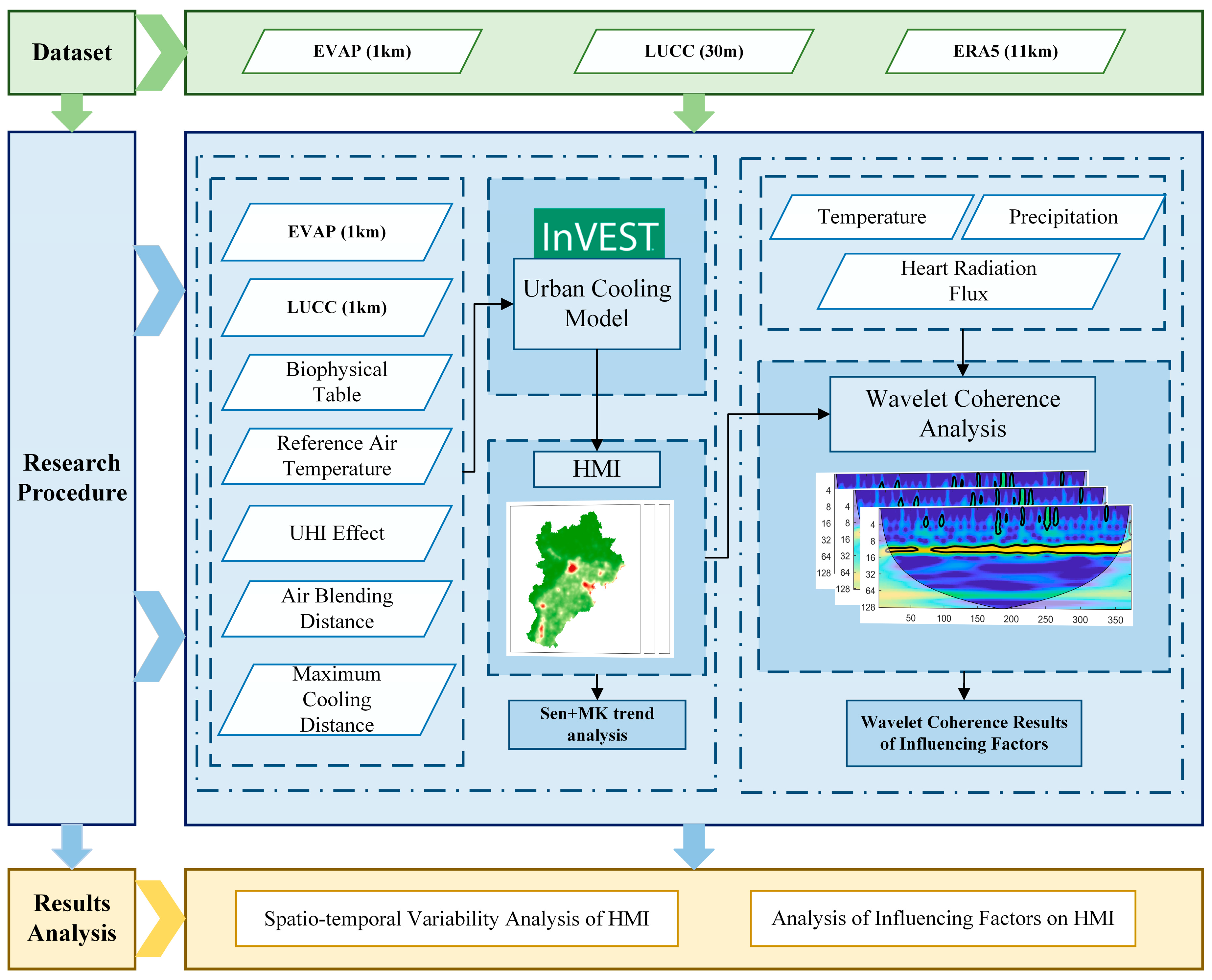
2. Data and Methodology

2.1. Study Area

The Beijing–Tianjin–Hebei urban agglomeration (36°00′–42°40′ N, 113°34′–120°05′ E) comprises two municipalities directly under the central government (Beijing and Tianjin) and a number of prefectural-level cities in Hebei Province [34]. The topography of the region is high in the northwest and low in the southeast, with plains and mountains dominating the terrain. The mountains concentrated in the northwest have abundant forest and grassland resources, as well as a better ecological environment, whereas the plains concentrated in the southeast have larger proportions of arable land and artificial surfaces and higher urbanization intensity. Figure 1 shows the rapid urbanization, crowding out of natural surfaces (e.g., water bodies and green spaces) by artificial impervious surfaces, and increasing anthropogenic heat emissions, which have led to the rapid development of the UHI effect [35]. Moreover, the emergence of urban agglomerations has strengthened inter-city linkages, thereby causing inter-city heat islands to overlap each other and further reinforcing the UHI effect [36]. This poses a threat to urban livability and sustainable development.

2.2. Data Sources

Multi-source satellite data sources were used as model input data, while reference data were used for statistical analysis (

Table 1. Datasets used in this study. Variables highlighted in green are input data required for the model, and those highlighted in blue are reference data used for statistical analysis.

Type	Dataset	Temporal Resolution	Time Range	Spatial Resolution
Evapotranspiration	1 km monthly potential evapotranspiration dataset in China (1901–2022) [37]	Monthly	1990–2020	1 km
Land cover	China Land Cover Dataset [38]	Annual	1990–2020	30 m
Air temperature Precipitation wind speed	ERA5-Land Monthly Aggregated—ECMWF Climate Reanalysis [39]	Monthly	1990–2020	11 km

). The evapotranspiration dataset was based on China’s 1 km monthly average, minimum, and maximum temperature data, and was calculated using the Hargreaves potential evapotranspiration formula. The land use dataset contained annual land cover information for China, with a spatial resolution of 30 m. The ERA5 climate reanalysis dataset, obtained from ECMWF, contained monthly surface air temperature data with an 11 km spatial resolution. The ERA5-Land reanalysis dataset was generated via the comprehensive processing of climate and initial weather data. To ensure consistency, the spatial resolution of all previously mentioned datasets was standardized to 1 km by resampling during data pre-processing. Annual-scale data were used for land use owing to its gradual changes; however, monthly data were used for the other variables.

2.3. Methods

A flowchart of the process followed in this study is shown in Figure 2. After data pre-processing, the InVEST UCM was utilized to assess the integrated heat reduction index of blue-green spaces in the study area for each year from 1990 to 2020. The intra- and inter-annual variations of the HMI of the composite blue-green spaces from 1990 to 2020 were analyzed, to which the wavelet coherence method was applied to explore the factors that influenced the modeled changes.

2.3.1. HMI Model

This study conducted a comprehensive assessment of the cooling capacity of regional blue-green spaces in China based on the UCM module of InVEST [28]. InVEST (v3.11.0) is an open-source software model jointly developed by Stanford University, the World Wildlife Fund, and The Nature Conservancy that is mainly used to quantify and assess ecosystem services and support decision-making. The UCM can quantify and map the cooling capacity index of each image element and consider the cooling effect of large green spaces (>2 ha) on the surroundings. In this case, terrestrial water bodies were considered to have the same cooling capacity as green spaces. The output of the model includes parameters such as the urban cooling index, image cooling capacity index, and estimated air temperature. In addition, InVEST provides open-source Python (3.9.12) APIs for functions such as UCM, which make long time-series and large-scale data batch processing feasible through these interface functions [40].

The core element in the UCM module is calculating the heat mitigation index (Urban Heat Mitigation, HM) for each pixel on the raster space. HM_i is the main output of the UCM. Its value ranges from 0 to 1, where 0 indicates that there is no cooling function in the cell and 1 indicates that the UHI has been completely mitigated. The definition of HMi is shown in Equation (1):

$${HM}_i=\left\{\begin{array}{cc}{CC}_i& if {CC}_i\ge {CC}_{{bg}_i} or {GA}_i<2ha\\ {CC}_{{bg}_i}& otherwise\end{array}\right\},$$

(1)

where i represents a particular pixel cell in the raster. If the pixel is not affected by large green spaces, then HM_i is equal to its own cooling capacity index (CC_i). If the large green space around the pixel is able to provide an additional cooling effect, then HM_i is equal to the weighted average of the cooling capacity of the green space and the distance of the cooling radiation (CCbg_i). GA_i is the area of the green space based on the search distance (dcool) around each pixel, which is calculated as in the following equation. The remaining components are calculated as defined in Equations (3)–(6).

$${GA}_i={cell}_{area}·\sum _{j\in d radius from i}{g}_j,$$

(2)

In Equation (2), cell_area is the area of the image element.

-

Cooling Capacity Index CC (Cooling Capacity)

The cooling capacity index (CC) is a quantitative measure of cooling capacity that estimates the cooling capacity of each pixel. The method is based on the indices proposed by Zardo et al., 2017 [41], and Kunapo et al., 2018 [29], with albedo, an important factor in heat reduction, further added to the model, as shown in Equation (3):

$${CC}_i=0.6·\mathrm{s}\mathrm{h}\mathrm{a}\mathrm{d}\mathrm{e}+0.2·\mathrm{a}\mathrm{l}\mathrm{b}\mathrm{e}\mathrm{d}\mathrm{o}+0.2·\mathrm{E}\mathrm{T}\mathrm{I}.$$

(3)

In Equation (3), CC_i represents the cooling capacity index of the current pixel. The weight of each pixel’s calculation method is based on the model’s recommended values, which reflect a higher impact of shade than evapotranspiration. The shade, taking the value 0–1, indicates the proportion of the canopy layer (≥2 m high) associated with each land use category. The specific value interval for each land use category is determined by synthesizing the sample data and the relevant literature and then taking the reference year’s shade value as the initial value for yearly adjustment, which is calculated as in Equation (4). The albedo indicates the proportion of solar radiation reflected by each land use type, and the specific value refers to the model sample data. ETI is the normalized value of potential evapotranspiration, i.e., evapotranspiration from vegetation (or soil evapotranspiration from unvegetated areas), calculated as in Equation (5).

$${shade}_i={shade}_k\left[1\pm \left(j·m\right)\right],$$

(4)

In Equation (4), shade_i denotes the shade factor in year i, k is the reference year, and j denotes the increase in year i from the reference year. m is the magnitude of the adjustment, which takes the value of 0.15 in Equation (4) and has an upward trend.

$$\mathrm{E}\mathrm{T}\mathrm{I}={\displaystyle \frac{K_c·ET0}{{ET}_{max}}},$$

(5)

In Equation (5), ET0 is the reference evapotranspiration provided to the model and K_c denotes the evapotranspiration coefficient of crops. The value interval of each land use type was determined with reference to the research results of Allen et al. (1998) [42], based on which, according to the different characteristics of each feature type, it was adjusted accordingly every year in the same way as in Equation (4). In this relationship, in the farmland, shrubs, and grassland land use types, m is taken as 0.003, which is an upward trend; for an impervious surface, m is taken as 0.003, which is a downward trend; and for the remaining land use types, m is taken as 0.001, which is an upward trend. ET_max is the maximum value of the ET0 raster, where the equation assumes that vegetated areas are adequately irrigated.

In Equation (1), CC_bgi is the cooling capacity of each image element under the additional cooling effect provided by the large green space around the pixel. The specific algorithm is shown in Equation (6).

$${CC}_{{bg}_i}=\sum _{j\in d radius from i}{g}_j·{CC}_j·e^{\left({\displaystyle \frac{-d\left(i,j\right)}{d_{cool}}}\right)},$$

(6)

In Equation (6), g_i is the pixel attribute, for which a value of 1 indicates green space and a value of 0 indicates something different. It is determined using the parameter “green spaces” in the biophysical table; d(i,j) is the distance between pixel i and pixel j and dcool is the range of cooling radiation, which is provided as a model input and has a value of 6 km.

2.3.2. Wavelet Analysis

Wavelet coherence is a mathematical method used to analyze the coherence of two signals at different times and scales. Wavelet coherence analysis quantifies the degree of correlation between two time series at different frequencies and different points in time by comparing their wavelet transforms.

In this study, the Morlet wavelet was chosen as the wavelet basis function. The Morlet wavelet is a widely used wavelet basis function especially suitable for time–frequency analysis. It is a combination of a complex exponential function and a Gaussian window function. The basic form of the Morlet wavelet can be expressed as follows:

$$\Psi \left(t\right)=\int {\pi }^{-1/4}{e}^{{iw}_{0}t}{e}^{{-t}^2/2},$$

(7)

In Equation (7), π^−1/4 is a normalization factor that ensures that the energy of the wavelet function is equal to 1. $e^{{iw}_{0}t}$ is a complex exponential function used to generate the oscillatory part, where i is an imaginary unit, t is a time variable, and ω₀ is the center frequency. $e^{{-t}^2/2}$ is the Gaussian window function, which is used to localize the wavelet function so that it has good localization properties in both time and frequency domains.

First, a continuous wavelet transform is applied to the two time series X(t) and Y(t) using Morlet wavelets.

$$W_X\left(i,j\right)=\int X\left(t\right){\Psi }_{i,j}^{*}\left(t\right)dt,$$

(8)

Equation (8) is the transform expression for X(t); Y(t) is transformed identically. In Equation (8), ${\Psi }_{i,j}^{*}$ is the complex conjugate wavelet function after scaling and translation, i is the scale parameter to control the scaling of the wavelet function, and j is the translation parameter to control the movement of the wavelet function along the time axis of the signal. $W_x\left(i,j\right)$ and $W_y\left(i,j\right)$ are the convolutions of the signals X(t) and Y(t) with the wavelet basis functions, which provide representations of the signals at different times and scales.

First, it is necessary to calculate the cross-wavelet spectrum, which reflects the common characteristics of the two time series at different scales i (frequencies) and times j. The cross-wavelet spectrum is calculated using the wavelet basis function. It is possible to determine when (time) and at which scales (frequency) the two signals exhibit interrelationships. It is calculated as follows:

$$W_{XY}\left(i,j\right)=W_X·W_Y^{*}\left(i,j\right),$$

(9)

In Equation (9), $W_Y^{*}\left(i,j\right)$ is the complex conjugate of $W_Y\left(i,j\right)$.

Next, the wavelet coherence coefficients are calculated.

$$R_{xy}^2\left(i,j\right)={\displaystyle \frac{{\left|\mathrm{S}\left(i,j\right)\left[W_{XY}\left(i,j\right)\right]\right|}^2}{\mathrm{S}\left(i,j\right)\left[{\left|W_X\left(i,j\right)\right|}^2\right]·\mathrm{S}\left(i,j\right)\left[{\left|W_Y\left(i,j\right)\right|}^2\right]}},$$

(10)

In Equation (10), $\mathrm{S}\left(i,j\right)$ denotes the smoothing operation at scale i and time j. The wavelet coherence coefficient $R_{xy}^2\left(i,j\right)$ has a value between 0 and 1 and is used to quantify the degree of correlation between two signals at a particular scale and point in time. Values close to 1 indicate a high degree of coherence. Finally, the results are interpreted and visualized [43].

Multiple wavelet coherence (MWC) is employed in signal processing and data analysis using multiple wavelet functions to better capture and characterize the complex features within a signal. For a response variable Y and multiple predictor variables X = (X₁, X₂, …, X_n), the definition of multiple wavelet coherence is as follows:

$${\rho }_M^2\left(s,\tau \right)={\displaystyle \frac{{\left|W^{Y,X}\left(s,\tau \right)\right|}^2}{W^{Y,X}\left(s,\tau \right)W^{Y,Y}\left(s,\tau \right)}},$$

(11)

In Equation (11), $W^{Y,X}\left(s,\tau \right)$ denotes the smoothed cross-wavelet power matrix between Y and X, $W^{X,X}\left(s,\tau \right)$ denotes the smoothed auto-wavelet and cross-wavelet power matrix among the multiple predictor variables, $W^{Y,Y}\left(s,\tau \right)$ is the smoothed wavelet power matrix of the response variable, and $W^{Y,X}\left(s,\tau \right)$ is the complex conjugate of $W^{Y,X}\left(s,\tau \right)$.

In the wavelet analysis, the 95% confidence level was obtained using Monte Carlo repeated calculations based on the first-order autocorrelation coefficient (1000 repetitions). The ability of the predictor variables to explain the response variables was assessed quantitatively by calculating the percentage of significant power (POSP) outside the wavelet cone of influence (WCI) and the average wavelet coherence (AWC). For combinations of variables, the addition of a new variable was considered statistically significant when it resulted in an increase in the POSP of at least 5% [44].

3. Results

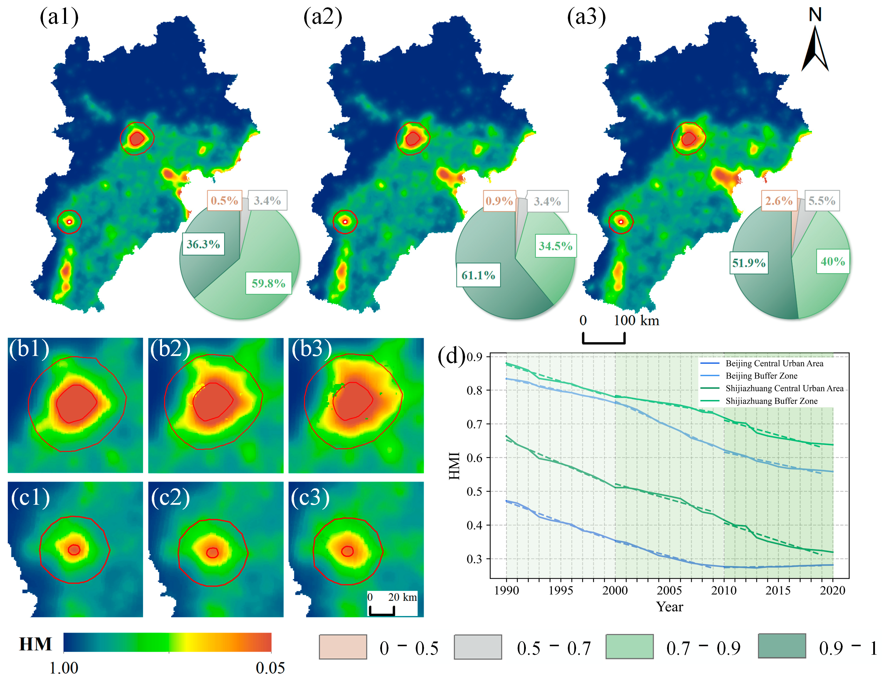
3.1. Temporal and Spatial Changes in HMI

The spatial distributions of the HMI were roughly similar in all years (Figure 3), with generally low values in the southeastern urban areas and high values in the northwestern mountainous areas, which corresponds with the distribution of blue-green spaces. The range of the low-value area expanded over time, whereas the range of the high-value area shrank over time. In addition, urban expansion and reductions in blue-green spaces caused the regional cooling capacity to weaken over time. The low-value point often corresponded with the location of the region’s center city, and its range and value were closely related to the level of urban development. As shown in Figure 3a, the range of low-value zones expanded outward over time, and the corresponding percentage of low-value zones has increased annually (from 0.5% in 1990–2000 to 2.6% at the end of the time series). In addition, the regional minimum value decreased from 0.3 to 0.05 over time.

Figure 3b,c show the HMI in the local Beijing and Shijiazhuang urban areas. To determine the range along the urban low-value area in 1990, a 24 km buffer zone was established to assess the spatiotemporal changes in the HMI in the urban center and urban outreach space. In this case, Beijing represents a first-tier type of city, whereas Shijiazhuang represents a second-tier type of city. Figure 3d shows the annual time-series graphs for the urban areas of Beijing and Shijiazhuang and their peripheral buffer zones. Overall, the rate of decrease was fast in the first two decades, but slowed in the second decade. In the first stage, the initial HMI value of the Beijing urban area was the lowest. The HMI values of Beijing and the peripheral buffer zone of Shijiazhuang were all greater than 0.8, with better spatial heat reduction effects, which corresponds to the state of urban development and the distribution of blue-green spaces at the time. In this stage, the HMI in urban areas decreased at a faster rate (with a slope of more than 0.01), which was closely related to an increased level of urbanization and the expansion of urban land areas. Such expansion reduced the area of blue-green spaces, thereby weakening the corresponding radiative cooling capacity of the blue-green spaces. The corresponding urban peripheral buffer zone during this stage decreased at a slower rate. In the second and third stages, the HMI values of the four regions varied. It is worth noting that the HMI decrease in the Beijing urban area during the second stage, slowed until the third stage, and then increased. The changes in the HMI in the Beijing urban area over the past three decades reflect the development of a typical metropolis, with rapid urbanization at the cost of ecological degradation during the early stages of development and more attention paid to ecological harmony and livability during the later stages. In addition, Beijing’s peripheral buffer zone decreased rapidly during the second stage, whereas the Shijiazhuang urban area maintained a high rate of decrease during the third stage. The development of the urban area’s peripheral buffer zone lagged behind that of the urban area. Similarly, secondary cities such as Shijiazhuang lagged behind pioneer cities such as Beijing.

3.2. Environmental Factors Affecting Cooling Capacity in Blue-Green Spaces

3.2.1. Relationships between Cooling Capacity and Individual Factors

Figure 4 shows the wavelet coherence of the blue-green space HMI with temperature, precipitation, and wind speed. The statistics are presented in

Table 2. Statistical analysis of the wavelet coherence between the HMI and individual environmental factors.

Wavelet Coherence	POSP (%)				AWC
	All	<8 d	8–16 d	>16 d	All	<8 d	8–16 d	>16 d
HMI–PRE	18.54	6.31	75.61	2.78	0.53	0.53	0.85	0.38
HMI–TEM	19.39	5.52	79.22	3.96	0.55	0.57	0.86	0.35
HMI–WS	17.54	11.65	61.69	1.51	0.55	0.58	0.79	0.39

(TEM: temperature; PRE: precipitation; WS: wind speed).

. The wavelet transform coherence (WTC) results indicate that the HMI exhibited significant coherence with the individual environmental factors at a specific time frequency throughout the study period. In this study, the time–frequency scales were divided into hourly (<8 d), medium (8–16 d), and large, (>16 d) time–frequency scales. The HMI and environmental factors had complex coherence at hourly time–frequency scales, with a constantly changing bit-phase angle. However, the bit-phase angle varied significantly and steadily at medium time–frequency scales. For the WTC, wind speed had the largest effect on the HMI at the hourly time–frequency scale, with an AWC of 0.58 and a POSP of 11.65. Thus, localized airflow patterns may be affected by changes in wind speed at shorter time scales and may change considerably, which directly affects the HMI. Therefore, the high coherence of wind speed and the spatial cooling index on short time scales may reflect this localized resonance phenomenon of airflow changes. At the medium time–frequency scale, all elements exhibited high coherences, with temperature having the greatest effect on the HMI (AWC of 0.86). Thus, seasonal and cyclical variations in weather systems have a substantial effect on the HMI. At all time–frequency scales, temperature was the best variable for explaining the variations in the HMI, with an AWC of 0.55 and a POSP of 19.39.

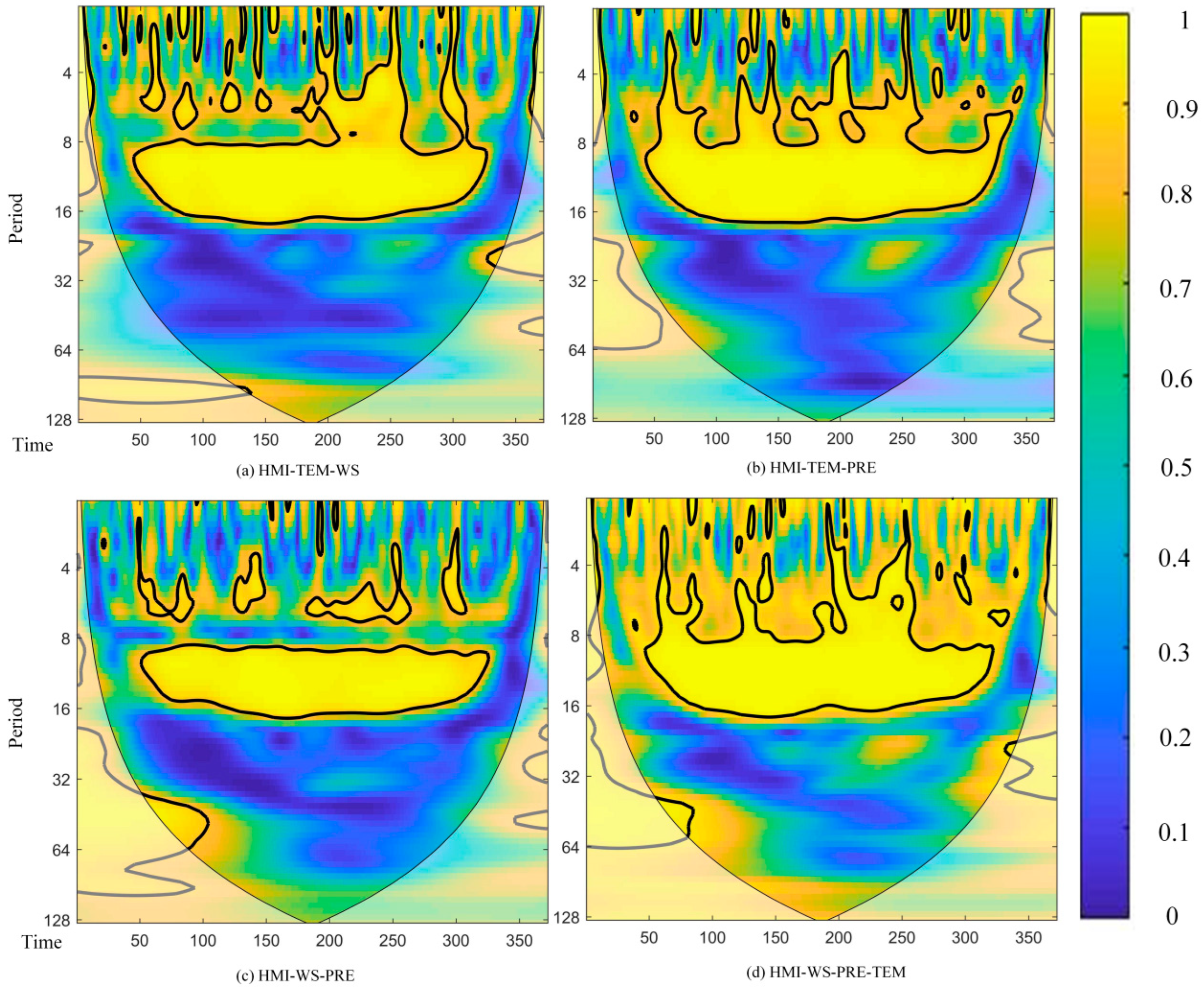
3.2.2. Relationships between Cooling Capacity and Multiple Environmental Factors

Because the influence of environmental factors on the cooling effect of blue-green spaces is always a comprehensive result of many factors, we explored the influences of multivariate combinations on the cooling effect. Figure 5 shows the MWC of the blue-green space HMI with temperature, precipitation and wind speed. The parameter statistics are listed in

Table 3. Statistical analysis of wavelet coherence between the HMI and multiple environmental factors.

Wavelet Coherence	POSP (%)				AWC
	All	<8 d	8–16 d	>16 d	All	<8 d	8–16 d	>16 d
HMI–TEM–WS	24.08	19.94	74.21	3.16	0.73	0.82	0.91	0.55
HMI–TEM–PRE	24.05	19.58	75.32	2.88	0.72	0.79	0.89	0.55
HMI–WS–PRE	17.79	9.04	62.3	4.63	0.69	0.72	0.88	0.56
HMI–WS–PRE–TEM	21.52	16.01	69.2	3.29	0.82	0.88	0.93	0.69

(TEM: temperature; PRE: precipitation; WS: wind speed).

. Substantial coherence was observed between the HMI and the three environmental factors, but significant differences occurred among the time–frequency domains. Overall, the AWCs for the same number of variable combinations were roughly similar on all time–frequency scales; however, the POSPs differed substantially. The HMI had complex correlations with the environmental factors on hourly time–frequency scales; however, on medium time–frequency scales, it was relatively stable and significant. The elements exhibited strong seasonal coherence, suggesting that the cooling effect of blue-green spaces is closely related to the meteorological conditions in a particular season. Moreover, sudden changes in environmental factors (or extreme events such as heat waves or heavy rain) can have an immediate effect on the cooling capacity of blue-green spaces. The variables did not exhibit significant interrelationships in the long-term trend, which may be the result of other long-term factors influencing the meteorological conditions (e.g., urbanization and climate change) on an annual scale that may weaken the coherence between the signals.

At the hourly time–frequency scale, different combinations of variables also had substantial differences. The best bivariate combinations that explained the changes in the HMI of blue-green spaces at the hourly time–frequency scale were temperature and wind speed. The coherence was highly substantial at the medium time–frequency scale, with a POSP of 74.21 and AWC of 0.91. The four-variable wavelet coherence had a stronger AWC (0.82) than that of the three-variable wavelet coherence at all time–frequency scales. In particular, the performance was more significant at the hourly time–frequency scale. The four variables interacted with each other, resulting in combinations that were indicative of co-variation patterns. For example, the radiative flux may directly affect the temperature and also the cooling capacity of blue-green spaces. Precipitation not only affects the moisture contents of blue-green spaces and thereby the cooling capacity, but also alters the energy balance at the surface. The POSP indicates the temporal phase relationships of the four elements, i.e., there were some temporal deviations in their peaks and troughs.

4. Discussion

4.1. Limitations of the Model

Although the InVEST UCM is widely used and optimized in the field, its application has some limitations that need to be resolved in future studies. For example, some key parameters in the model (e.g., maximum cooling and air mixing distances of the blue-green space) need to be adjusted according to the geographic and climatic characteristics, which vary with vegetation characteristics, climate, and wind direction. This is the main limitation of the model when considering the uncertainty of the effect of horizontal convection on temperature homogenization [45]. In addition, the model defines parameters such as shade, Kc, and albedo based on land use type; therefore, the model’s analytical accuracy is closely related to the level of detail in the land use data classification, making it difficult to distinguish between buildings, vegetation, and other features. Finally, an assessment of the health impacts of the UHI effect is important but is not currently included in the model, owing to wide variations among different cities [46].

Input data errors can also affect the model results. The optimized UFORE model used in this study relies on multiple remote sensing data sources (e.g., ERA5, land cover, and evapotranspiration data), and inversion errors of the products of the respective data sources may affect the computational accuracy of the final results. Moreover, the products have differing spatial and temporal resolutions. Although these errors are minimized by algorithms and technical means, the data applicability and accuracy still have potential impacts on the final model results.

The complexity of the urban environment is also a limiting factor. In addition to the environmental elements covered in Section 3.2, many urban morphological features can lead to differing distributions of the UHI effect both locally and globally, including the influences of buildings, different ground material types, and anthropogenic heat sources, which may not be fully considered by the model. This limitation affects the results of the assessment of the cooling effect. Furthermore, the InVEST model mainly assesses static ecological services, but the cooling effect of urban blue-green spaces is strongly influenced by seasonality and weather conditions. Thus, the InVEST model may not adequately capture these dynamic changes. Although the use of the InVEST model with satellite remote sensing data is a powerful tool, these limitations must be considered in specific applications, and other data sources and methods should be combined with the model to improve the accuracy and applicability of its output.

4.2. Urban Blue-Green Spatial Planning

Globally, the application of blue-green infrastructure for mitigating the UHI effect has been successful. By analyzing advanced cases from various countries, several common characteristics have emerged in the use of blue-green infrastructure to reduce urban temperatures. First, greening has been integrated with buildings, with representative elements including green roofs, green walls, and rooftop gardens. For example, New York’s High Line and Paris’s Cité Universitaire International Student City are equipped with green roofs and walls, which effectively mitigate the UHI effect through plant transpiration [47]. Second, the multi-functionality of blue-green infrastructure has been emphasized, such as rain gardens. For example, Philadelphia’s “Green City, Clean Waters” program promotes rain gardens, which also beautify the environment and provide recreational spaces for the community. Third, adapting to local environmental features was a key focus of the present study. For example, Copenhagen emphasizes integrating drainage systems with greenery to cope with frequent rainfall events, while Singapore focuses on reducing temperatures in its hot and humid environment through extensive greening [48]. Finally, considering the long-term sustainability of cities is necessary for ensuring that blue-green infrastructure can continue to function effectively under future climate change. Programs such as Copenhagen’s urban adaptation plan and Singapore’s “Garden City” initiative not only address current climate conditions but also consider future extreme weather events [49].

Figure 6 shows the area of blue-green spaces in the Beijing–Tianjin–Hebei region, which has continuously decreased over time. Overall, the layout of blue-green spaces in urban areas is severely fragmented, as they are substantially constrained by the expansion of built-up areas. Therefore, the cooling functions of these spaces and the region’s environmental characteristics should be considered fully when planning blue-green spaces in the study region with the goal of reducing temperatures. The findings of this study indicate that large blue-green spaces can radiate cooling effects to their surrounding areas. In addition, the mountainous areas in the northwestern part of the study area contain large expanses of natural vegetation. Better protection of existing natural blue-green spaces is an effective measure for reducing urban temperatures. In addition, considering the study region’s recent precipitation patterns, wind conditions, and seasonal drought issues, the design of blue-green spaces within cities should include good drainage and water retention functions, which can enhance water resource utilization efficiency through facilities such as rain gardens. By taking advantage of the relatively high wind speeds in the study area, the strategic layout of green spaces and water bodies can guide air circulation and increase natural ventilation, thereby enhancing cooling effects. Owing to dense buildings and limited green spaces, the central urban areas of key cities in the study area had low blue-green space cooling capacities. In areas with high building density, blue-green spaces can be integrated using vertical greening systems, green roofs, and other approaches.

5. Conclusions

Global climate change and rapid urbanization profoundly affect the urban thermal environment and pose a threat to the sustainable development of cities. Quantitatively analyzing the spatiotemporal changes in the cooling effect of blue-green spaces and its influencing factors is crucial for mitigating the UHI effect and improving urban thermal comfort. We quantitatively analyzed the long-term cooling capacity of urban blue-green spaces in the Beijing–Tianjin–Hebei urban agglomeration and explored the changes in the cooling capacity during rapid urbanization. We then analyzed the main factors influencing the observed changes. The conclusions of the study are as follows:

(1)

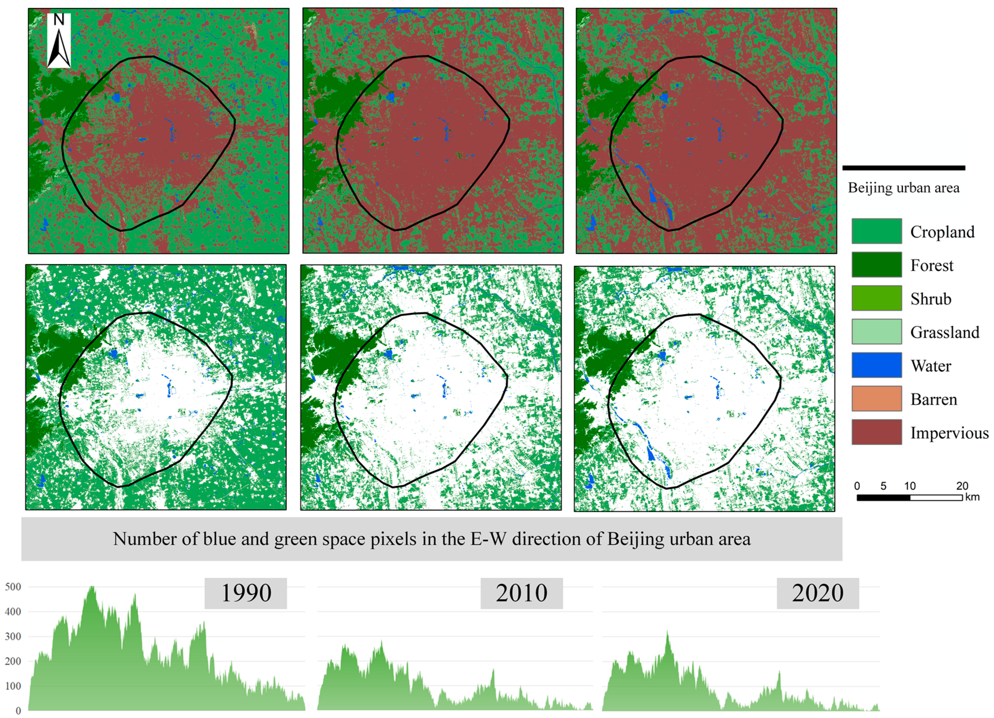
Low HMI values in the Beijing–Tianjin–Hebei region from 1990 to 2020 were mainly distributed in the various central cities in the region. In addition, the stage in which the time-series change occurred was remarkably important. In particular, the average HMI of the urban area of Beijing decreased by 0.2 during the study period (decreased rapidly in the early stage, slowed in the late stage, and exhibited a small upward trend during 2010–2020). The cities and districts in the study area were in different stages of development during the same period of time. The primary driver behind the observed changes was the persistent impact of urban expansion and corresponding blue-green space reduction.

(2)

The HMI exhibited coherence with environmental factors that was mainly reflected at the hourly time–frequency scale. The main factors controlling the HMI varied on different time–frequency scales. Overall, the inclusion of four variables demonstrated the best coherence (AWC of 0.82). These variables were the most effective explanatory variables for changes in the HMI. The individual variable that best explained the changes in the HMI was air temperature, while the best bivariate combination was air temperature and wind speed.

(3)

When planning blue-green spaces, it is particularly important to consider air temperature, precipitation, and wind speed to improve the sustainability of a city and the comfort of its residents. It is possible to establish cool microclimate zones, reduce surface temperatures, and mitigate the UHI effect by concentrating multi-layered greenery in hot spots, installing rain gardens and permeable paving, considering wind channel design, and using highly reflective materials and green roofs.

References

1. Gong, P.; Liu, H.; Zhang, M.; Li, C.; Wang, J.; Huang, H.; Clinton, N.; Ji, L.; Li, W.; Bai, Y.; et al. Stable Classification with Limited Sample: Transferring a 30-m Resolution Sample Set Collected in 2015 to Mapping 10-m Resolution Global Land Cover in 2017. Sci. Bull. 2019, 64, 370–373. [Google Scholar] [CrossRef] [PubMed]
2. Mirzaei, P.A. Recent Challenges in Modeling of Urban Heat Island. Sustain. Cities Soc. 2015, 19, 200–206. [Google Scholar] [CrossRef]
3. Huang, C.; Xu, N. Quantifying Urban Expansion from 1985 to 2018 in Large Cities Worldwide. Geocarto. Int. 2022, 37, 18356–18371. [Google Scholar] [CrossRef]
4. Estoque, R.C.; Murayama, Y.; Myint, S.W. Effects of Landscape Composition and Pattern on Land Surface Temperature: An Urban Heat Island Study in the Megacities of Southeast Asia. Sci. Total Environ. 2017, 577, 349–359. [Google Scholar] [CrossRef] [PubMed]
5. Yang, L.; Qian, F.; Song, D.-X.; Zheng, K.-J. Research on Urban Heat-Island Effect. Procedia. Eng. 2016, 169, 11–18. [Google Scholar] [CrossRef]
6. Kamath, H.G.; Martilli, A.; Singh, M.; Brooks, T.; Lanza, K.; Bixler, R.P.; Coudert, M.; Yang, Z.-L.; Niyogi, D. Human Heat Health Index (H3I) for Holistic Assessment of Heat Hazard and Mitigation Strategies beyond Urban Heat Islands. Urban Clim. 2023, 52, 101675. [Google Scholar] [CrossRef]
7. Santamouris, M.; Ding, L.; Fiorito, F.; Oldfield, P.; Osmond, P.; Paolini, R.; Prasad, D.; Synnefa, A. Passive and Active Cooling for the Outdoor Built Environment—Analysis and Assessment of the Cooling Potential of Mitigation Technologies Using Performance Data from 220 Large Scale Projects. Sol. Energy 2017, 154, 14–33. [Google Scholar] [CrossRef]
8. Chen, S.; Bao, Z.; Ou, Y.; Chen, K. The Synergistic Effects of Air Pollution and Urban Heat Island on Public Health: A Gender-Oriented Nationwide Study of China. Urban Clim. 2023, 51, 101671. [Google Scholar] [CrossRef]
9. Ou, Y.; Bao, Z.; Ng, S.T.; Song, W.; Chen, K. Land-Use Carbon Emissions and Built Environment Characteristics: A City-Level Quantitative Analysis in Emerging Economies. Land Use Policy 2024, 137, 107019. [Google Scholar] [CrossRef]
10. Pritipadmaja, P.; Garg, R.; Sharma, A. Assessing the Cooling Effect of Blue-Green Spaces: Implications for Urban Heat Island Mitigation. Water 2023, 15, 2983. [Google Scholar] [CrossRef]
11. Zhou, D.; Bonafoni, S.; Zhang, L.; Wang, R. Remote Sensing of the Urban Heat Island Effect in a Highly Populated Urban Agglomeration Area in East China. Sci. Total Environ. 2018, 629, 415–429. [Google Scholar] [CrossRef] [PubMed]
12. Carvalho, D.; Martins, H.; Marta-Almeida, M.; Rocha, A.; Borrego, C. Urban Resilience to Future Urban Heat Waves under a Climate Change Scenario: A Case Study for Porto Urban Area (Portugal). Urban Clim. 2017, 19, 1–27. [Google Scholar] [CrossRef]
13. Huang, C.; Xu, N. Climatic Factors Dominate the Spatial Patterns of Urban Green Space Coverage in the Contiguous United States. Int. J. Appl. Earth Obs. Geoinf. 2022, 107, 102691. [Google Scholar] [CrossRef]
14. Beauchamp, P.; Adamowski, J. An Integrated Framework for the Development of Green Infrastructure: A Literature Review. Eur. J. Sustain. Dev. 2013, 2, 1. [Google Scholar] [CrossRef]
15. Sinnett, D.; Jerome, G.; Burgess, S.; Smith, N.; Mortlock, R. Building with Nature—A New Benchmark for Green Infrastructure. Town Ctry. Plan. 2017, 86, 427–431. [Google Scholar]
16. Houkai, W.E.I.; Meng, N.; Le, L.I. China’s Strategies and Policies for Regional Development During the Period of the 14th Five-Year Plan. Chin. J. Urban Environ. Stud. 2020, 8, 2050008. [Google Scholar] [CrossRef]
17. Fan, J.; Xiao, Z. Analysis of Spatial Correlation Network of China’s Green Innovation. J. Clean. Prod. 2021, 299, 126815. [Google Scholar] [CrossRef]
18. Xu, N.; Lu, H.; Li, W.; Gong, P. Natural Lakes Dominate Global Water Storage Variability. Sci. Bull. 2024, 69, 1016–1019. [Google Scholar] [CrossRef]
19. Huang, M.; Cui, P.; He, X. Study of the Cooling Effects of Urban Green Space in Harbin in Terms of Reducing the Heat Island Effect. Sustainability 2018, 10, 1101. [Google Scholar] [CrossRef]
20. Yu, Z.; Yang, G.; Zuo, S.; Jørgensen, G.; Koga, M.; Vejre, H. Critical Review on the Cooling Effect of Urban Blue-Green Space: A Threshold-Size Perspective. Urban For. Urban Green. 2020, 49, 126630. [Google Scholar] [CrossRef]
21. Jiang, Y.; Huang, J.; Shi, T.; Li, X. Cooling Island Effect of Blue-Green Corridors: Quantitative Comparison of Morphological Impacts. Int. J. Environ. Res. Public Health 2021, 18, 11917. [Google Scholar] [CrossRef] [PubMed]
22. Şimşek, Ç.K.; Serter, G.; Ödül, H. A Study on the Cooling Capacities of Urban Parks and Their Interactions with the Surrounding Urban Patterns. Appl. Spat. Anal. 2022, 15, 1287–1317. [Google Scholar] [CrossRef]
23. Sheng, S.; Wang, Y. Configuration Characteristics of Green-Blue Spaces for Efficient Cooling in Urban Environments. Sustain. Cities Soc. 2024, 100, 105040. [Google Scholar] [CrossRef]
24. Quan, S.; Li, M.; Li, T.; Liu, H.; Cui, Y.; Liu, M. Nonlinear Effects of Blue-Green Space Variables on Urban Cold Islands in Zhengzhou Analyzed with Random Forest Regression. Front. Ecol. Evol. 2023, 11, 1185249. [Google Scholar] [CrossRef]
25. Xue, X.; He, T.; Xu, L.; Tong, C.; Ye, Y.; Liu, H.; Xu, D.; Zheng, X. Quantifying the Spatial Pattern of Urban Heat Islands and the Associated Cooling Effect of Blue–Green Landscapes Using Multisource Remote Sensing Data. Sci. Total Environ. 2022, 843, 156829. [Google Scholar] [CrossRef]
26. Amani-Beni, M.; Zhang, B.; Xie, G.-D.; Shi, Y. Impacts of Urban Green Landscape Patterns on Land Surface Temperature: Evidence from the Adjacent Area of Olympic Forest Park of Beijing, China. Sustainability 2019, 11, 513. [Google Scholar] [CrossRef]
27. Zhou, W.; Cao, W.; Wu, T.; Zhang, T. The Win-Win Interaction between Integrated Blue and Green Space on Urban Cooling. Sci. Total Environ. 2023, 863, 160712. [Google Scholar] [CrossRef] [PubMed]
28. Hamel, P.; Guerry, A.D.; Polasky, S.; Han, B.; Douglass, J.A.; Hamann, M.; Janke, B.; Kuiper, J.J.; Levrel, H.; Liu, H.; et al. Mapping the Benefits of Nature in Cities with the InVEST Software. npj Urban Sustain. 2021, 1, 25. [Google Scholar] [CrossRef]
29. Kunapo, J.; Fletcher, T.D.; Ladson, A.R.; Cunningham, L.; Burns, M.J. A Spatially Explicit Framework for Climate Adaptation. Urban Water J. 2018, 15, 159–166. [Google Scholar] [CrossRef]
30. Zawadzka, J.E.; Harris, J.A.; Corstanje, R. Assessment of Heat Mitigation Capacity of Urban Greenspaces with the Use of InVEST Urban Cooling Model, Verified with Day-Time Land Surface Temperature Data. Landsc. Urban Plan. 2021, 214, 104163. [Google Scholar] [CrossRef]
31. Battemarco, B.P.; Tardin-Coelho, R.; Veról, A.P.; de Sousa, M.M.; da Fontoura, C.V.T.; Figueiredo-Cunha, J.; Barbedo, J.M.R.; Miguez, M.G. Water dynamics and blue-green infrastructure (BGI): Towards risk management and strategic spatial planning guidelines. J. Clean. Prod. 2022, 333, 129993. [Google Scholar] [CrossRef]
32. Ji, L.; Shu, C.; Gaur, A.; Wang, L.; Lacasse, M. A State-of-the-Art Review of Studies on Urban Green Infrastructure for Thermal Resilient Communities. Build. Environ. 2024, 111524. [Google Scholar] [CrossRef]
33. Jiang, Y.; Huang, J.; Shi, T.; Wang, H. Interaction of Urban Rivers and Green Space Morphology to Mitigate the Urban Heat Island Effect: Case-Based Comparative Analysis. Int. J. Environ. Res. Public Health 2021, 18, 11404. [Google Scholar] [CrossRef] [PubMed]
34. Wu, A.-B.; Chen, F.-G.; Zhao, Y.-X.; Qin, Y.-J.; Liu, X.; Guo, X.-P. Multi-scenario Simulation of Construction Land Expansion and Its Impact on Ecosystem Carbon Storage in Beijing-Tianjin-Hebei Urban Agglomeration. Huan Jing Ke Xue 2024, 45, 2828–2839. [Google Scholar] [CrossRef] [PubMed]
35. Fang, C.L. Important Progress and Prospects of China’s Urbanization and Urban Agglomeration in the Past 40 Years of Reform and Opening-Up. Econ. Geogr 2018, 38, 1–9. [Google Scholar]
36. Wang, Z.; Liu, M.; Liu, X.; Meng, Y.; Zhu, L.; Rong, Y. Spatio-Temporal Evolution of Surface Urban Heat Islands in the Chang-Zhu-Tan Urban Agglomeration. Phys. Chem. Earth Parts A/B/C 2020, 117, 102865. [Google Scholar] [CrossRef]
37. Peng, S. 1 km Monthly Potential Evapotranspiration Dataset in China (1990–2021); National Tibetan Plateau Data Center: Beijing, China, 2022. [Google Scholar]
38. Yang, J.; Huang, X. The 30&thinsp;m Annual Land Cover Dataset and Its Dynamics in China from 1990 to 2019. Earth Syst. Sci. Data 2021, 13, 3907–3925. [Google Scholar] [CrossRef]
39. Muñoz-Sabater, J.; Dutra, E.; Agustí-Panareda, A.; Albergel, C.; Arduini, G.; Balsamo, G.; Boussetta, S.; Choulga, M.; Harrigan, S.; Hersbach, H.; et al. ERA5-Land: A State-of-the-Art Global Reanalysis Dataset for Land Applications. Earth Syst. Sci. Data 2021, 13, 4349–4383. [Google Scholar] [CrossRef]
40. Sharp, R.; Tallis, H.T.; Ricketts, T.; Guerry, A.D.; Wood, S.A.; Chaplin-Kramer, R.; Nelson, E.; Ennaanay, D.; Wolny, S.; Olwero, N.; et al. InVEST—Integrated Valuation of Ecosystem Services and Tradeoffs; Stanford University: Stanford, CA, USA, 2016. [Google Scholar]
41. Zardo, L.; Geneletti, D.; Pérez-Soba, M.; Van Eupen, M. Estimating the Cooling Capacity of Green Infrastructures to Support Urban Planning. Ecosyst. Serv. 2017, 26, 225–235. [Google Scholar] [CrossRef]
42. Allen, R.G.; Pereira, L.S.; Raes, D.; Smith, M. Crop Evapotranspiration: Guidelines for Computing Crop Requirements. FAO Irrig. Drain. Pap. 1998, 300, D05109. [Google Scholar]
43. Hu, W.; Si, B. Technical Note: Improved Partial Wavelet Coherency for Understanding Scale-Specific and Localized Bivariate Relationships in Geosciences. Hydrol. Earth Syst. Sci. 2021, 25, 321–331. [Google Scholar] [CrossRef]
44. Su, L.; Miao, C.; Duan, Q.; Lei, X.; Li, H. Multiple-Wavelet Coherence of World’s Large Rivers With Meteorological Factors and Ocean Signals. J. Geophys. Res. Atmos. 2019, 124, 4932–4954. [Google Scholar] [CrossRef]
45. Koc, C.B.; Osmond, P.; Peters, A. Evaluating the Cooling Effects of Green Infrastructure: A Systematic Review of Methods, Indicators and Data Sources. Sol. Energy 2018, 166, 486–508. [Google Scholar] [CrossRef]
46. McDonald, R.; Kroeger, T.; Boucher, T.; Longzhu, W.; Salem, R.; Adams, J.; Bassett, S.; Edgecomb, M.; Garg, S. Planting Healthy Air: A Global Analysis of the Role of Urban Trees in Addressing Particulate Matter Pollution and Extreme Heat; The Nature Conservancy: Arlington, VA, USA, 2016. [Google Scholar]
47. Jamei, E.; Thirunavukkarasu, G.; Chau, H.W.; Seyedmahmoudian, M.; Stojcevski, A.; Mekhilef, S. Investigating the cooling effect of a green roof in Melbourne. Build. Environ. 2023, 246, 110965. [Google Scholar] [CrossRef]
48. Kim, C.U.; Ryu, Y.H.; O, N.C.; Ri, J.N. A rainwater harvesting system in buildings with green roofs and a rooftop greenhouse in Pyongyang. Int. J. Environ. Sci. Technol. 2023, 20, 12295–12306. [Google Scholar] [CrossRef]
49. Harun, Z.; Akkurt, N.; Khor, Y.K.; Abbas, A.A.; Lotfy, E.R. Urban heat island patterns in garden cities: Putrajaya as a case study. Indoor Built Environ. 2024, 1420326X241244459. [Google Scholar] [CrossRef]
Figure 1. (a) Map of the Beijing–Tianjin–Hebei region. (b) Temporal and spatial changes in built-up areas, (c) surface temperature changes, (d) land cover, and (e) proportions of built-up areas and blue-green spaces.
Land 13 01423 g001
Figure 2. Flowchart of the procedures applied in this study.
Land 13 01423 g002
Figure 3. Distributions and spatial changes in the heat mitigation index (HMI) in the (a1a3) Beijing–Tianjin–Hebei region, (b1b3) local Beijing, and (c1c3) Shijiazhuang urban areas from 1990 to 2020. (d) Annual time-series graphs of the Beijing and Shijiazhuang urban areas and their peripheral buffer zones (each decade is defined as a stage).
Land 13 01423 g003
Figure 4. Wavelet correlations between blue-green space cooling effects and environmental factors (TEM: temperature; PRE: precipitation; WS: wind speed).
Land 13 01423 g004
Figure 5. Multi-wavelet coherence (MWC) of blue-green space HMI with multiple environmental factors (TEM: temperature; PRE: precipitation; WS: wind speed).
Land 13 01423 g005
Figure 6. Temporal and spatial changes in blue-green spaces in the Beijing–Tianjin–Hebei region.
Land 13 01423 g006