Evaluation of a Multivariate Calibration Model for the WET Sensor That Incorporates Apparent Dielectric Permittivity and Bulk Soil Electrical Conductivity

Abstract

The measurement of apparent dielectric permittivity (ε_s) by low-frequency capacitance sensors and its conversion to the volumetric water content of soil (θ) through a factory calibration is a valuable tool in precision irrigation. Under certain soil conditions, however, ε_s readings are substantially affected by the bulk soil electrical conductivity (EC_b) variability, which is omitted in default calibration, leading to inaccurate θ estimations. This poses a challenge to the reliability of the capacitance sensors that require soil-specific calibrations, considering the EC_b impact to ensure the accuracy in θ measurements. In this work, a multivariate calibration equation (multivariate) incorporating both ε_s and EC_b for the determination of θ by the capacitance WET sensor (Delta-T Devices Ltd., Cambridge, UK) is examined. The experiments were conducted in the laboratory using the WET sensor, which measured θ, ε_s, and EC_b simultaneously over a range of soil types with a predetermined actual volumetric water content value (θ_m) ranging from θ = 0 to saturation, which were obtained by wetting the soils with four water solutions of different electrical conductivities (EC_i). The multivariate model’s performance was evaluated against the univariate CAL and the manufacturer’s (Manuf) calibration methods with the Root Mean Square Error (RMSE). According to the results, the multivariate model provided the most accurate θ estimations, (RMSE ≤ 0.022 m³m⁻³) compared to CAL (RMSE ≤ 0.027 m³m⁻³) and Manuf (RMSE ≤ 0.042 m³m⁻³), across all the examined soils. This study validates the effects of EC_b on θ for the WET and recommends the multivariate approach for improving the capacitance sensors’ accuracy in soil moisture measurements.

1. Introduction

Efficient precision irrigation as a fundamental component of natural resource sustainability requires advanced sensing systems with easy maintenance and robust procedures for the collection and assimilation of soil moisture data. In this regard, the determination of soil moisture is accomplished in real time with contemporary electromagnetic (EM) sensors that provide continuous measurements of the volumetric water content of soil, θ (m³m⁻³), in the field. The majority of the currently available EM soil moisture devices are based on the dielectric properties of soil and include technologies like Time Domain Reflectometry (TDR) and Frequency Domain Reflectometry (FDR) or capacitance, impedance, and Amplitude Domain Reflectometry (ADR) [1].

Among them, the portable capacitance sensors are considered a suitable and affordable option for the interpretation of the spatiotemporal distribution of soil moisture in automated monitoring networks [2,3,4].

Dielectric properties-based techniques have been broadly adopted as an effective and rapid means to acquire in situ, nondestructive, and point-scale measurements of soil water content. The principle underlying these methods relies on the soil dielectric permittivity, an intrinsic soil property that allows soil to polarize and retain an electrical charge in response to the electric field induced by a sensor. Soil dielectric permittivity, ${\mathsf{\epsilon }}_{\mathrm{r}}^{*}$, is a complex, dimensionless unit that consists of a real and an imaginary part, expressed as

$${\mathsf{\epsilon }}_{\mathrm{r}}^{*}={\mathsf{\epsilon }}_{\mathrm{r}}^{\prime }-\mathrm{j}{\mathsf{\epsilon }}_{\mathrm{r}}^{″}$$

(1)

where the real component or dielectric constant of the soil, ${\mathsf{\epsilon }}_{\mathrm{r}}^{\prime }$, reflects the stored electrical energy in the medium, while the imaginary component, ${\mathsf{\epsilon }}_{\mathrm{r}}^{″}$, indicates the energy dissipation with j = $\sqrt{-1}$. The energy losses denoted by ${\mathsf{\epsilon }}_{\mathrm{r}}^{″}$ are associated to the bulk soil electrical conductivity, EC_b (dSm⁻¹), and the molecular relaxation processes, ${\mathsf{\epsilon }}_{\mathrm{r}\mathrm{e}\mathrm{l}}^{″}$ [5], as presented in

$${\mathsf{\epsilon }}_{\mathrm{r}}^{″}={\mathsf{\epsilon }}_{\mathrm{r}\mathrm{e}\mathrm{l}}^{″}+{\displaystyle \frac{\mathrm{E}{\mathrm{C}}_{\mathrm{b}}}{2\mathsf{\pi }f{\mathsf{\epsilon }}_0}}$$

(2)

where f is the frequency of the electromagnetic field (Hz), and ${\mathsf{\epsilon }}_0$ is the free space permittivity. The soil’s dielectric behavior implies that the sensors operating frequency and EC_b have a profound impact on the apparent dielectric permittivity of the soil, ε_s, which is measured by all the dielectric sensors and is aligned with the combination of ${\mathsf{\epsilon }}_{\mathrm{r}}^{\prime }$ and${\mathsf{\epsilon }}_{\mathrm{r}}^{″}$ [6]. Hence, in TDR systems that operate at frequencies exceeding 1 GHz, the dielectric loss factor, ${\mathsf{\epsilon }}_{\mathrm{r}}^{″}$, is negligible, and ${\mathsf{\epsilon }}_{\mathrm{r}}^{\prime }$ is equal to ε_s [7,8]. On the contrary, in lower frequencies, the dependency of ${\mathsf{\epsilon }}_{\mathrm{r}}^{″}$ on EC_b has significant implications on ε_s measurements [9]. Overall, as the operation frequency increases, ε_s tends to decrease.

Given that ε_s is characterized by a remarkably higher value for free water (ε_s ≈ 80) at 20 °C than it is for solid constituents (ε_s = 2–5) and air (ε_s = 1) in soil, it is substantially dependent on the volumetric soil water content, θ [10]. In order to quantify the relationship between ε_s and θ, several calibration models have been developed over the years, including additional soil parameters like the soil’s temperature and the soil’s bulk density [11].

One of the most well-known and extensively used calibration models is the third-order polynomial equation of Topp et al. [12] (Equation (3)) for the case of TDR [13].

$$\mathsf{\theta }=-5.3\times {10}^{-2}+2.92\times {10}^{-2}{\mathsf{\epsilon }}_{\mathrm{s}}-5.5\times {10}^{-4}{\mathsf{\epsilon }}_{\mathrm{s}}^2-4.3\times {10}^{-6}{\mathsf{\epsilon }}_{\mathrm{s}}^3$$

(3)

This non-linear model, referred to as the Topp equation, and its versatile formulations have been demonstrated to be applicable for various dielectric sensors [9,14,15]; however, the model’s precision is limited to coarse-textured mineral soils.

A linear approach (Equation (4)), commonly called the refractive index model [16] of the form

$$\mathsf{\theta }=\mathrm{a}\sqrt{{\mathsf{\epsilon }}_{\mathrm{s}}}+\mathrm{b}$$

(4)

with a and b curve-fitting parameters, has also gained widespread acceptance for being a simpler, equivalent equation of Topp’s [9,17,18,19]. Many commercial ΕΜ probes employ this univariate model as a factory default to calculate θ, since the linearity of θ − $\sqrt{{\mathsf{\epsilon }}_{\mathrm{s}}}$ is proven to be valid for a range of inorganic soil types, moisture, and salinity conditions and the a and b coefficients are either factory-fixed for textural classes or can be easily determined. In this respect, with a and b values of 0.115 and −0.176, respectively, Topp and Reynolds [20] provided good results using the TDR approach up to θ = 0.45 m³m⁻³, with deviations of less than 0.01 m³m⁻³ from the Topp equation (Equation (3)).

As a matter of fact, for the prediction of θ, the efficacy of the single-variable models can be compromised in saline and clayey soils due to the high values of EC_b that influence the electromagnetic wave signals. The complex interactions of EC_b with soil properties such as soil water content, soil texture, clay type, salinity, cation exchange capacity, and temperature illustrate a combined effect on ε_s measurements, which cannot be distinguished when monitoring volumetric water content in the field [21]. The variability of EC_b as a consequence of soil heterogeneity may lead to erroneous measurements of ε_s and ultimately to systematically biased soil water content readings. This impact is more pronounced at impedance and capacitance probes with operational frequencies below 200 MHz and particularly at 1–50 MHz, where electrical conductivity emerges as the most crucial mechanism of dielectric dissipation [21,22,23,24,25].

Low-frequency sensors, like the WET capacitance probe (Delta-T Devices Ltd., Cambridge, UK) that operates at 20 MHz, have been documented to be more susceptible to EC_b changes and tend to overestimate ε_s when the electrical conductivity levels of the soil increase, resulting in overestimated θ values [14,26,27,28,29]. According to Kargas et al. [30], the performance of the WET drastically decreases for EC_b values above 3 dSm⁻¹, while other authors report this threshold to be approximately 2.5 dSm⁻¹ for different capacitance probes [8,31]. Furthermore, the soil types with a high clay content result in the overestimation of ε_s values as the frequency decreases [23,30,32]. Under such soil conditions, a soil-specific calibration employing correction functions or mathematical models to compensate for the EC_b effects is essential for enhancing the accuracy of capacitance and impedance sensors.

Robinson et al. [33], using two capacitance devices, proposed an empirical correction equation that relates the square root of the real part of the ε_s, $\sqrt{{\mathsf{\epsilon }}_{\mathrm{r}}^{\prime }}$, and EC_b for predicting θ. Regarding the results, the function provides sufficient estimations for sandy soils and EC_b values up to 2.5 dSm⁻¹. Using soil water reflectometers, the equation was later reported to be applicable for higher EC_b levels, outperforming the default calibration but exhibiting overall low accuracy [34].

Examining the performance of the 5TE (70 MHz) capacitance probe (Decagon Devices, Pullman, WA, USA) on laboratory and field conditions, Zemni et al. [35] found that the permittivity-corrected linear model of Kargas et al. [25], which integrates the effect of EC_b on ε_s, increases the accuracy of θ compared to the default calibration model of Topp’s for EC_b ≤ 0.75 dSm⁻¹.

Evett et al. [36], based on TDR data, developed a multivariate model that accounts for the effects of soil texture and salinity on θ determination, using the $\sqrt{{\mathsf{\epsilon }}_{\mathrm{s}}}$ and $\sqrt{{\mathrm{E}\mathrm{C}}_{\mathrm{b}}}$ as independent variables. Similarly, Kargas and Soulis, [34] utilizing experimental data obtained by the CS655 sensor, proposed an alternative modification to the multivariate model for the evaluation of θ that incorporates $\sqrt{{\mathsf{\epsilon }}_{\mathrm{s}}}$ and EC_b values. The latter model appears to be more physically realistic, due to the fact that the values of the partial slope for EC_b are negative and those for the partial slope of $\sqrt{{\mathsf{\epsilon }}_{\mathrm{s}}}$ are positive in all cases. Additionally, the values of their slopes tend to the corresponding values proposed by Topp and Reynolds [20].

The performance of the aforementioned multivariate models has been explored along with other well-known single-ε_s variable models for a series of soil water reflectometers. A CS65x (Cambpbell Scientific Inc., Logan, UT, USA), operating at a frequency of around 175 MHz in diverse soil conditions, indicated satisfactory results [7,34,37]. For instance, Patrignani et al. [37], investigated the calibration of the CS655 soil moisture sensor across nine soil textural classes and various EC_b values of up to 3.1 dSm⁻¹. They reported the multivariate model of Kargas and Soulis to be the most accurate calibration equation in estimating θ, with a Root Mean Square Error of RMSE = 0.033 cm³cm⁻³ and the lowest mean absolute error among various univariate models and the multivariate model of Evett et al. [36]. Moreover, through the conduction of intensive field surveys, the authors of the current study previously identified the implementation of the Kargas and Soulis model as an acceptable option for the spatiotemporal monitoring of soil moisture, eliminating the need for site-specific calibrations. This multivariate model, that includes both EC_b and $\sqrt{{\mathsf{\epsilon }}_{\mathrm{s}}}$, was also shown to adequately correct the strong temperature effects on ε_s of the CS655 in clayey soils and increased soil water contents.

More recently, Wilson et al. [21] applied both the models of Kargas and Soulis [34] and Evett et al. [36] to assess the variability of EC_b on θ measurements obtained by the impedance Hydra probe (50 MHz). As they documented, the inclusion of EC_b noticeably improves the θ estimations in fine clay and saline soils, contrary to the manufacturer-supplied calibration.

Even though the necessity of soil-specific calibration to optimize the accuracy of θ measurements has been addressed in the literature, the evaluation of the existing multivariate calibration models that consider the EC_b’s effects has been confined to a rather narrow spectrum of low-frequency dielectric sensors.

In this aspect, the objective of this study is to investigate the accuracy of the multivariate calibration model of Kargas and Soulis [34] on the volumetric soil water content estimations using EC_b and ε_s measurements obtained by the popular and low-cost capacitance WET sensor (20 MHz). The performance of the multivariate approach is compared and evaluated against the classic univariate (CAL) calibration and the manufacturer (Manuf) calibration across a range of soil types, moisture conditions, and salinity conditions.

2. Materials and Methods

2.1. The WET Sensor

The WET sensor (Delta-T Devices Ltd., Cambridge, UK), which belongs to the FDR category, is a capacitance dielectric sensor of low cost that, when operating at a frequency of 20 MHz, measures directly and simultaneously the bulk soil electrical conductivity (EC_b), the apparent soil dielectric permittivity (ε_s), and the temperature (T). The sensor consists of three 6.8 cm-long stainless rods with 3 mm diameters that, when inserted into the medium, measure the capacitance and the conductance by generating a 20 MHz electromagnetic signal between the rods. This signal is applied to the central rod that is related to the EC_b and the soil temperature and is then sent to the connected HH2 data logger. Besides the dielectric properties, the sensor also estimates the volumetric water content and the pore water electrical conductivity using the Hilhorst model [38].

The calculation of the volumetric soil water content, θ, from the measurements of ε_s that are obtained by the WET is conducted using the simplified linear equation of Topp (Equation (4)) and its fitting parameters, a and b.

The slope (a) of the regression equation of Topp is influenced by the soil type and soil salinity while the intercept (b) is related to the electrical properties of the solid components of the soil [39].

Since the soil type affects the measurements of θ, the manufacturer suggests a calibration be applied in accordance with the provided fixed set of parameter values for more accurate results. In the case of mineral soils, the proposed values of a and b are 0.099 and −0.178, respectively, whereas for organic soils and sands, a = 0.119 and b = −0.167. For clay soils, the values are a = 0.091 and b = −0.182 [40].

2.2. Experimental Soils and the Characterization of Their Physical Properties

For the execution of the laboratory experiments, seven mineral-porous media including three sandy loam soils (SL 1, SL 2, SL 3), a clay loam soil (CL), a loam soil (L), a sandy soil (S), and a clay soil (C) were collected from various fields in Greece and used in the study to acquire a variety of textural classes from fine to coarse soils (

Table 1. Soil textural fractions and bulk densities (ρ_b) of the examined soils.

Soil	Sand	Silt	Clay	Bulk Density (ρb)
	(%)	(%)	(%)	(g cm−1)
SL 1—Sandy Loam 1	57.0	26.5	16.5	1.44
SL 2—Sandy Loam 2	51.8	30.0	18.2	1.38
SL 3—Sandy Loam 3	67.8	16.0	16.2	1.52
CL—Clay Loam	35.8	36.0	28.2	1.25
S—Sand	100	-	-	1.68
L—Loam	40.6	35.6	23.8	1.15
C—Clay	24.5	20.5	55.0	1.16

). The diversity of soil types attempts to facilitate the investigation of the sensor’s response in heterogenous soil conditions and enhance the performance evaluation of the examined calibration models.

The collected disturbed soil samples were air-dried, sieved through a 2 mm sieve, and further processed in the laboratory to determine their physical properties and, more specifically, the soils’ textural fractions and dry bulk densities (ρ_b). The Bouyoucos method was applied for the soil texture analysis, while for the bulk density, a subsample of each soil was put into the oven for over-drying at 105 °C for 24 h and then the bulk density was calculated based on the mass and volume of the dry soil.

The results from the analyses are presented in Table 1.

2.3. Measurements of Volumetric Soil Water Content, Apparent Dielectric Permittivity, and EC_b under Different Salinity Levels (EC_i)

In this study, the performance of the WET sensor on θ estimations and its sensitivity to variations in soil salinity were investigated for all the examined soils, in the laboratory. The experiments for the collection of the required data were carried out across a range of predetermined moisture contents from oven-dry to saturation and increasing salinity levels of 0.28, 1.2, 3, 6 dSm⁻¹.

In particular, a specific mass of the air-dried soil samples was weighed and placed in glass beakers. For every soil sample, a predefined quantity of tap water, which has an electrical conductivity (EC_i) of 0.28 dSm⁻¹, was added each time to increase the actual measured volumetric water content (θ_m) in constant steps of θ = 0.05 m³m⁻³ up to near saturation. Each addition of a certain amount was thoroughly mixed with the soil sample to ensure a uniform moisture distribution throughout the mixture. Hence, for each soil, a set of beakers with soil mixtures of different moisture levels were prepared.

Subsequently, all the obtained soil mixtures were packed in plastic columns in small portions and compressed with a 0.15 kg rubber hammer to achieve a homogeneous bulk density in the soil columns. After their equilibration for 24 h in airtight conditions, the WET was inserted vertically into the soil columns without touching the bottom or the sides of the column, and the output readings were taken with the HH2 data logger. Furthermore, measurements were taken in oven-dried soil samples (θ_m = 0 m³m⁻³).

To evaluate the response of the sensor to soil salinity effects, the described process was repeated using predetermined KCl solutions with a known electrical conductivity, EC_i of 1.2, 3, or 6 dSm⁻¹ each, which were applied individually instead of tap water.

All the experiments were conducted at constant temperature (23 ± 1 °C) to avoid temperature effects.

Through the above methodology, a sufficient number of measurements for volumetric soil water content (θ), apparent dielectric permittivity (ε_s), and soil bulk electrical conductivity (EC_b) were acquired by the WET under different moisture conditions and salinity levels (EC_i) for all the studied soils.

2.4. Calibration Models of Volumetric Water Content for WET Sensor

2.4.1. Manufacturer Calibration (Manuf)

Initially, the volumetric water content, θ, of the WET sensor is evaluated by the default equation (Equation (4)) and the a and b values that were proposed by the manufacturer in the operator’s manual for the mineral (a = 0.099, b = −0.178), clay (a = 0.091, b = −0.182), and sand (a = 0.119, b = −0.167) soils. This process hereafter in the study is referred to as manufacturer calibration (Manuf).

2.4.2. Univariate Calibration Model (CAL)

To examine the possible improvement of the WET sensor’s accuracy in θ estimations, a soil-specific calibration on the default equation (Equation (4)) was employed. Particularly, soil-specific values for the a and b parameters were determined by constructing a linear regression between the measured θ_m and the corresponding $\sqrt{{\mathsf{\epsilon }}_{\mathrm{s}}}$ values, using all the measured θ_m from oven-dry to saturation [34]_. By this means, optimal pairs of a and b values were acquired for the entire range of θ at each salinity level (EC_i) and for all the soils studied. The linear fitting method to the θ_m $-\sqrt{{\mathsf{\epsilon }}_{\mathrm{s}}}$ relationship that calculated the a and b parameters to predict θ was noted in the study as the classic univariate CAL calibration.

2.4.3. Multivariate Calibration Model Considering the EC_b Effects

To assess and evaluate the effects of EC_b on the volumetric water content (θ) by the WET probe, the Kargas and Soulis [34] model was applied to all the tested soils.

The particular model, mentioned as multivariate hereafter, determines θ by the ε_s and EC_b as follows:

$$\mathsf{\theta }=\mathrm{a}\sqrt{{\mathsf{\epsilon }}_{\mathrm{s}}}+\mathrm{b}+\mathrm{c}\mathrm{E}{\mathrm{C}}_{\mathrm{b}}$$

(5)

where a, b, and c are the fitting parameters. In this case, the calibration of θ for each soil and salinity level was developed by applying a multiple linear regression analysis to the θ_m values and the corresponding $\sqrt{{\mathsf{\epsilon }}_{\mathrm{s}}}$ and EC_b data. The analysis and determination of all the coefficients a, b and c were conducted in the SPSS statistical software (version 22.0, SPSS Inc., Chicago, IL, USA).

The multivariate equation is considered a more realistic calibration in contrast to other multivariate models, since it demonstrates how to capture the physical relationship among $\sqrt{{\mathsf{\epsilon }}_{\mathrm{s}}}$, EC_b, and θ in diverse soil conditions. Concerning the soil water reflectometers, the model interprets a strong relationship among the three variables with relative accuracy [21,37], thus indicating a good potential method for calibrating the WET sensor and improving its performance in θ estimations.

2.5. Performance Evaluation Criteria

The performance of the multivariate model, along with the calibrations of CAL and Manuf, is evaluated using the Root Mean Square Error

$$\mathrm{R}\mathrm{M}\mathrm{S}\mathrm{E}=\sqrt{{\displaystyle \frac{1}{\mathrm{n}}}{\mathsf{\Sigma }}_{\mathrm{i}=1}^{\mathrm{n}}{\left(\mathrm{P}\mathrm{r}\mathrm{e}{\mathrm{d}}_{\mathrm{i}}-\mathrm{O}\mathrm{b}{\mathrm{s}}_{\mathrm{i}}\right)}^2}$$

(6)

that allows us to quantify the accuracy of the investigated calibration equations. Pred_i refers to the values of the volumetric water content, θ, predicted by the calibration models for the i-th value, while Obs_i is the corresponding measured θ_m value for the total of n predicted–observed values. RMSE is expressed in the same units as the predicted values (m³m⁻³) and indicates a better model performance with lower values closer to zero.

Moreover, the adjusted coefficient of determination (Adj. R²) was used to examine the relationships between the θ_m and the variables of $\sqrt{{\mathsf{\epsilon }}_{\mathrm{s}}}$ and EC_b of the univariate and the multivariate model for the WET sensor:

$$\mathrm{A}\mathrm{d}\mathrm{j}.{\mathrm{R}}^2=1-\left[{\displaystyle \frac{{\sum }_{\mathrm{i}=1}^{\mathrm{n}}{\left(\mathrm{O}\mathrm{b}{\mathrm{s}}_{\mathrm{i}}-\mathrm{P}\mathrm{r}\mathrm{e}{\mathrm{d}}_{\mathrm{i}}\right)}^2∕\left(\mathrm{n}-\mathrm{k}-1\right)}{{\sum }_{\mathrm{i}=1}^{\mathrm{n}}{\left(\mathrm{O}\mathrm{b}{\mathrm{s}}_{\mathrm{i}}-\left(\mathrm{m}\mathrm{e}\mathrm{a}\mathrm{n}\mathrm{O}\mathrm{b}{\mathrm{s}}_{\mathrm{i}}\right)\right)}^2∕\left(\mathrm{n}-1\right)}}\right]$$

(7)

where k is the number of the fitting parameters and n is the total number of data points. Adj. R² values that are close to 1 reflect a stronger correlation.

The metric of the Akaike Information Criteria (AIC_c), corrected for the small sample size, was also applied in the SPSS software to compare the goodness of fit between the models while accounting for parsimony. The AIC_c considers the balance between the model fit and the complexity by penalizing additional parameters. In addition, to quantify the relative differences between the estimated AIC_c values, the delta AIC (ΔAIC_c) was computed. The specific equations for these criteria are as follows:

$${\mathrm{AIC}}_{\mathrm{c}}=2\mathrm{k}-2\ln (\mathrm{L})+{\displaystyle \frac{2\mathrm{k}\left(\mathrm{k}+1\right)}{\mathrm{n}-\mathrm{k}-1}}$$

(8)

ΔAIC_c = ΔAIC_c i − ΔAIC_c min

(9)

where k is the number of the model’s parameters and L is the maximum likelihood for the model; ΔAIC_c i is the model being compared and ΔAIC_c min is the model with the lowest AIC_c value.

Smaller AIC_c values indicate better models and ΔAIC_c = 0 represents the best fitting model.

3. Results and Discussion

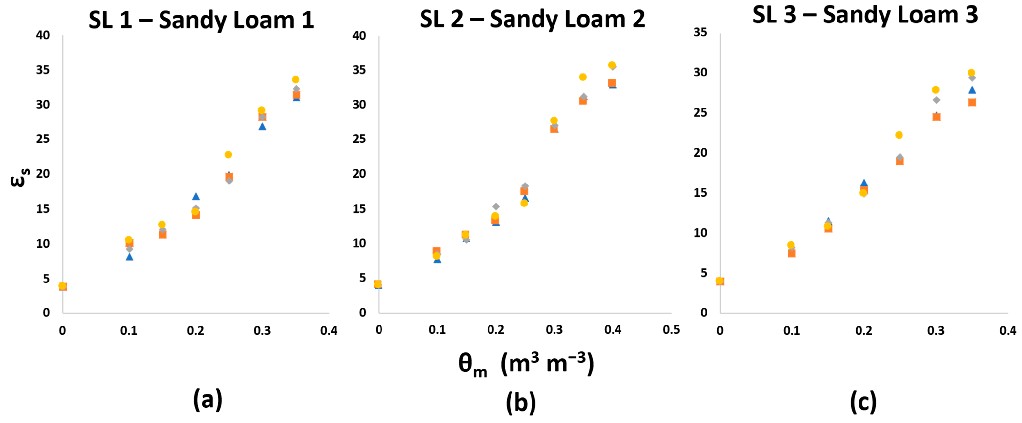
3.1. Relationship of Apparent Dielectric Permittivity and Volumetric Water Content

The relationship between the apparent dielectric permittivity, ε_s, as determined by the WET sensor and the actual volumetric soil water content, θ_m, for all the examined porous media and salinity levels (EC_i) is illustrated in Figure 1.

As can been seen in Figure 1, for the same θ_m, the ε_s of WET increases consistently with the increasing EC_i from 0.28 to 6 dSm⁻¹ for all the soils, implying the influence of the higher salinity levels on the low-frequency sensor’s response. The increasing ε_s with the increase of soil salinity becomes more evident in θ_m values above 0.3 m³m⁻³, where the discrepancies among the measured ε_s are larger from the lowest to the highest EC_i.

In accordance with Figure 1, the Adj. R² values, which were assessed for the univariate and the multivariate relationships to evaluate the fit between the variables, are depicted in

Table 2. The values a and b of the linear θ_m $-\sqrt{{\mathsf{\epsilon }}_{\mathrm{s}}}$ and the a, b, and c values of the θ_m $-\sqrt{{\mathsf{\epsilon }}_{\mathrm{s}}}-$ EC_b relationships with their corresponding Adj. R² values for all the examined soils and salinity levels (EC_i). The maximum EC_b values at saturation are also included.

Soil	ECi (dSm−1)	CAL			Multivariate				Max ECb (dSm−1)
		${\mathsf{\theta }}_{\mathbf{m}}=\mathbf{a}\sqrt{{\mathsf{\epsilon }}_{\mathbf{s}}}+\mathbf{b}$			${\mathsf{\theta }}_{\mathbf{m}}=\mathbf{a}\sqrt{{\mathsf{\epsilon }}_{\mathbf{s}}}+\mathbf{b}+\mathbf{c}\mathbf{E}{\mathbf{C}}_{\mathbf{b}}$
		a	b	Adj. R2	a	b	c	Adj. R2
SL 1—Sandy Loam 1	0.28	0.094	−0.176	0.993	0.129	−0.255	−0.146	0.995	0.81
	1.2	0.094	−0.177	0.975	0.117	−0.232	−0.087	0.976	0.94
	3	0.093	−0.175	0.986	0.117	−0.232	−0.072	0.987	1.18
	6	0.090	−0.174	0.979	0.098	−0.194	−0.018	0.979	1.63
SL 2—Sandy Loam 2	0.28	0.097	−0.171	0.971	0.230	−0.469	−0.894	0.990	0.52
	1.2	0.100	−0.187	0.978	0.146	−0.295	−0.221	0.980	0.74
	3	0.096	−0.176	0.988	0.118	−0.232	−0.077	0.988	1.12
	6	0.091	−0.156	0.960	0.129	−0.252	−0.090	0.964	1.56
SL 3—Sandy Loam 3	0.28	0.102	−0.200	0.993	0.188	−0.378	−0.572	0.994	0.48
	1.2	0.103	−0.196	0.986	0.157	−0.313	−0.287	0.987	0.56
	3	0.097	−0.184	0.991	0.126	−0.251	−0.105	0.993	0.90
	6	0.093	−0.172	0.981	0.112	−0.218	−0.047	0.981	1.38
CL—Clay Loam	0.28	0.097	−0.165	0.938	0.201	−0.419	−0.544	0.964	0.74
	1.2	0.100	−0.180	0.948	0.158	−0.194	−0.260	0.952	0.90
	3	0.101	−0.182	0.964	0.146	−0.299	−0.155	0.970	1.20
	6	0.092	−0.160	0.963	0.130	−0.266	−0.090	0.969	1.78
S—Sand	0.28	0.133	−0.207	0.996	0.165	−0.265	−0.921	0.999	0.09
	1.2	0.123	−0.191	0.997	0.150	−0.244	−0.271	0.998	0.29
	3	0.119	−0.193	0.998	0.124	−0.204	−0.025	0.999	0.72
L—Loam	0.28	0.095	−0.162	0.962	0.159	−0.314	−0.486	0.973	0.52
	1.2	0.091	−0.154	0.977	0.140	−0.274	−0.273	0.990	0.73
	3	0.090	−0.164	0.980	0.119	−0.237	−0.103	0.985	1.18
	6	0.086	−0.153	0.966	0.111	−0.222	−0.066	0.970	1.77
C—Clay	0.28	0.109	−0.254	0.985	0.182	−0.450	−0.505	0.988	0.59
	1.2	0.112	−0.259	0.976	0.162	−0.396	−0.266	0.980	0.82
	3	0.108	−0.243	0.970	0.144	−0.349	−0.131	0.972	1.28
	6	0.097	−0.228	0.986	0.100	−0.238	−0.007	0.987	1.95

for all the tested soils and salinity levels. The values of the a and b fitting parameters for the θ_m $-\sqrt{{\mathsf{\epsilon }}_{\mathrm{s}}}$ and the calculated a, b, and c of the θ_m $-\sqrt{{\mathsf{\epsilon }}_{\mathrm{s}}}-$ EC_b relationships along with the maximum EC_b values at saturation are also included.

The high Adj. R² values from Table 2 indicate that the θ_m $-\sqrt{{\mathsf{\epsilon }}_{\mathrm{s}}}$ relationship is strongly linear in all the cases examined, validating the linearity of the refractive index model (Equation (4)) for the WET sensor. More specifically, the obtained Adj. R² values (Table 2) range from 0.938 to 0.998 for all the soils and salinity levels, EC_i up to 6 dSm⁻¹. The greatest Adj. R² values are observed in S soil, ranging from 0.996 at EC_i = 0.28 dSm⁻¹ to 0.998 for EC_i = 3 dSm⁻¹, while the linear relationship yields the smallest Adj. R² value (Adj. R²= 0.938) in the CL soil, at EC_i = 0.28 dSm⁻¹. The linearity between θ_m and $\sqrt{{\mathsf{\epsilon }}_{\mathrm{s}}}$ for the WET sensor has been also reported in other studies [30].

Regarding the slope (a) of the linear θ_m $-\sqrt{{\mathsf{\epsilon }}_{\mathrm{s}}}$relationship at all the salinity levels, the average value for the mineral soils (SL 1, SL 2, CL, and L) is a = 0.093; for C soil the value ranges from 0.097 to 0.112, and the values are between 0.119 and 0.133 for the S. The empirical value of a is close to the corresponding value proposed by the manufacturer for mineral soils (a = 0.099) when using the default calibration (Equation (4)). Nonetheless, in the case of C, the calculated a values are higher than the manufacturer’s calibration (a = 0.091) for the clay soils at all EC_i, indicating the high effect of the clay content on the WET’s ε_s measurements. For the S soil, the slopes are closer to the factory-supplied value (a = 0.119) at the higher EC_i levels of 3 and 6 dSm⁻¹, whereas for EC_i = 0.28 dSm⁻¹, the value of a is relatively higher (a = 0.133).

In addition to the parameters of a, the average estimated intercept (b) of the θ_m $-\sqrt{{\mathsf{\epsilon }}_{\mathrm{s}}},$in mineral soils (b = −0.169) tends to be the corresponding recommended value of the manufacturer calibration (b = −0.178). A similar trend to the slopes was observed for the calculated b values in the cases of the C and S soils.

According to the findings of Table 2, the multivariate equation relating $\sqrt{{\mathsf{\epsilon }}_{\mathrm{s}}}$, EC_b, and θ_m exhibits a great fit to the measured data, with Adj. R² values ranging from 0.952 to 0.999 across all the soils, the salinity levels up to 6 dSm⁻¹, and the maximum EC_b values up to 1.95 dSm⁻¹. The substantially high Adj. R² signifies the strong relationship of θ_m $-\sqrt{{\mathsf{\epsilon }}_{\mathrm{s}}}$− EC_b under the examined soil conditions of the study.

The maximum EC_b values attained at saturation did not exceed 2 dSm⁻¹ at the highest EC_i = 6 dSm⁻¹; hence, they are below the threshold of 3 dSm⁻¹, above which the WET response has been reported to deteriorate.

As concerns the fitting parameters of the multivariate model, the partial slopes of $\sqrt{{\mathsf{\epsilon }}_{\mathrm{s}}}$ (a) are positive, while the intercepts (b) and the partial slopes of EC_b (c) are negative in all the cases. The observation of the negative values of c associated with EC_b, as determined by the WET sensor, comes to an agreement with the results of Kargas and Soulis [34] and Patrignani et al. [37], who investigated the multivariate model for the soil water reflectometers across a wide range of soil types.

The resulting signs of the a, b, and c fitting parameters of the multivariate equation confirm the physically dynamic relationship of the volumetric soil water content with ε_s and EC_b at the variations of soil salinity.

Furthermore, it was observed that the average values of a obtained by the multivariate model are higher than those of the univariate’s model (CAL) in all the soils examined, while the average b values are consistently lower. In fact, for the mineral soils, the partial slope of $\sqrt{{\mathsf{\epsilon }}_{\mathrm{s}}}$ and the intercept have average values of a = 0.135 and b = −0.263, respectively, while the corresponding average values for the CAL are a = 0.093 and b = −0.169. Similarly, in C soil, the average values are a = 0.147 and b = −0.358, whereas the average values of the univariate are a = 0.106 and b = −0.246. In S soil, the multivariate exhibits the average values of a and b as 0.146 and −0.238, respectively, while the corresponding average values of the univariate are a = 0.125 and b = −0.197.

3.2. Evaluation of the Multivariate Model in Comparison to Manuf and CAL Calibration for the Prediction of θ

The accuracy of the multivariate model in predicting the volumetric soil water content, θ, was evaluated and compared to the factory’s supplied calibration (Manuf) of WET and the univariate (CAL) method in RMSE terms for all the examined soils and salinity levels, EC_i.

Table 3. The RMSE values of the volumetric soil water content (θ) predictions obtained by the manufacturer (Manuf) calibration of the WET sensor, the classic univariate (CAL) procedure, and the multivariate model of Kargas and Soulis, [34] for each soil and salinity level (EC_i). The average RMSE for each soil is also provided.

Soil	ECi (dSm−1)	Manuf		CAL $\mathsf{\theta }=\mathbf{a}\sqrt{{\mathsf{\epsilon }}_{\mathbf{s}}}+\mathbf{b}$		Multivariate $\mathsf{\theta }=\mathbf{a}\sqrt{{\mathsf{\epsilon }}_{\mathbf{s}}}+\mathbf{b}+\mathbf{c}\mathbf{E}{\mathbf{C}}_{\mathbf{b}}$
		RMSE (m3m−3)	Average	RMSE (m3m−3)	Average	RMSE (m3m−3)	Average
SL 1—Sandy Loam 1	0.28	0.021	0.028	0.008	0.013	0.006	0.012
	1.2	0.026		0.016		0.015
	3	0.026		0.012		0.011
	6	0.037		0.015		0.014
SL 2—Sandy Loam 2	0.28	0.020	0.021	0.020	0.018	0.011	0.014
	1.2	0.018		0.017		0.015
	3	0.018		0.013		0.012
	6	0.028		0.023		0.020
SL 3—Sandy Loam 3	0.28	0.013	0.016	0.008	0.011	0.007	0.010
	1.2	0.013		0.012		0.010
	3	0.016		0.010		0.008
	6	0.024		0.014		0.013
CL—Clay Loam	0.28	0.031	0.029	0.031	0.027	0.022	0.022
	1.2	0.029		0.028		0.025
	3	0.024		0.024		0.020
	6	0.031		0.025		0.021
S *—Sand	0.28	0.013	0.019	0.007	0.006	0.004	0.003
	1.2	0.015		0.006		0.002
	3	0.028		0.004		0.004
L—Loam	0.28	0.024	0.036	0.024	0.020	0.018	0.016
	1.2	0.022		0.018		0.011
	3	0.053		0.017		0.014
	6	0.043		0.022		0.020
C—Clay	0.28	0.048	0.042	0.025	0.025	0.023	0.022
	1.2	0.039		0.020		0.014
	3	0.049		0.027		0.025
	6	0.029		0.021		0.021

* For EC_i = 6 dSm⁻¹ the response of the WET was not evaluated.

demonstrates the obtained RMSE as well as the average RMSE values of θ by each model.

Considering an acceptable accuracy level of RMSE = 0.03 m³m⁻³ [34], it can be seen in Table 3 that the use of Manuf calibration leads to a poor accuracy of θ in the fine-textured soils. In practice, the highest RMSE values are observed in the L (average RMSE = 0.036 m³m⁻³) and C soils (average RMSE = 0.042 m³m⁻³).

Contrary to the factory calibration (Manuf), both the univariate CAL and multivariate models show more accurate predictions, with the average RMSE values below 0.027 m³m⁻³ for all soils.

More specifically, the CAL calibration provides reasonable θ estimations (0.006 ≤ average RMSE ≤ 0.027 m³m⁻³), indicating a better performance than the corresponding average RMSE values of the Manuf calibration (0.016 ≤ average RMSE ≤ 0.042 m³m⁻³). Nevertheless, the prediction performance of the univariate model is still lower than that of the multivariate model, which demonstrates the highest accuracy (0.003 ≤ average RMSE ≤ 0.022 m³m⁻³) across all the experimental soils. It is noteworthy that except for the SL 3 and CL soils, the multivariate reduces the average RMSE by almost 50% in comparison to the corresponding average RMSE values of the default calibration.

As reported in Table 3, the multivariate RMSE values range from 0.002 to 0.025 m³m⁻³ for all the salinity levels (EC_i) with the smallest values included in the S soil (0.002 ≤ RMSE ≤ 0.004 m³m⁻³). The highest RMSE value of 0.025 m³m⁻³ is found in the CL and C soils at EC_i = 1.2 and 3 dSm⁻¹, respectively, while the corresponding RMSE values of the Manuf calibration for the same soils and the respective electrical conductivities are 0.029 and 0.049 m³m⁻³. Especially in the C soil, the increased RMSE values of the manufacturer calibration at all salinity levels up to 6 dSm⁻¹ (RMSE ranged from 0.029 to 0.049 m³m⁻³) resulted in the highest average RMSE = 0.042 m³m⁻³ across the entire dataset. This value, however, drops to an average RMSE = 0.022 m³m⁻³ when employing the multivariate calibration, implying that the effects of the increased clay content on the ε_s and EC_b measurements can be sufficiently corrected with the multivariate model that takes them into account for θ calculations. Moreover, for the L soil, the calculated RMSE values of the multivariate calibration at EC_i = 3 (RMSE = 0.014 m³m⁻³) and 6 dSm⁻¹ (RMSE = 0.020 m³m⁻³) are remarkably lower and nearly half of the corresponding RMSE values of the factory calibration (RMSE = 0.053 and 0.043 m³m⁻³, respectively). Hence, in these salinity levels, the calibration recommended by the manufacturer failed to estimate θ accurately.

The results derived from the evaluation of the applied calibrations (Table 3) highlight the significance of considering the EC_b effects on the soil water content estimations by the WET sensor. The multivariate approach, using both ε_s and EC_b measurements, outperforms (average RMSE ≤ 0.022 m³m⁻³) the factory calibration (Manuf) (average RMSE ≤ 0.042 m³m⁻³) and the calibration of CAL (average RMSE ≤ 0.027 m³m⁻³) that relies solely on ε_s in all the cases.

To further evaluate the predictive capability of the multivariate model, a goodness-of-fit comparison between the univariate and the multivariate model was conducted using the corrected Akaike Information Criteria (AIC_c). The AIC_c values of each model, which were calculated by averaging the AIC_c values of all the salinity levels for each soil, are listed in

Table 4. The AIC_c and the delta AIC_c (ΔAIC_c) values of the univariate and multivariate models for each soil.

Soil	CAL	Multivariate	ΔAICc CAL *	ΔAICc Multivariate *
	${\mathsf{\theta }}_{\mathbf{m}}=\sqrt{{\mathsf{\epsilon }}_{\mathbf{s}}}+\mathbf{b}$	${\mathsf{\theta }}_{\mathbf{m}}=\mathbf{a}\sqrt{{\mathsf{\epsilon }}_{\mathbf{s}}}+\mathbf{b}+\mathbf{c}\mathbf{E}{\mathbf{C}}_{\mathbf{b}}$
	AICc	AICc
SL 1—Sandy Loam 1	−36.92	−35.40	2	0
SL 2—Sandy Loam 2	−38.68	−35.83	3	0
SL 3—Sandy Loam 3	−39.62	−37.58	2	0
CL—Clay Loam	−32.97	−30.33	3	0
S—Sand	−41.64	−38.72	3	0
L—Loam	−61.31	−54.29	7	0
C—Clay	−33.96	−32.15	2	0

* ΔAIC_c: The difference between the AIC_c of the model being compared and the model with the lowest AIC_c. ΔAIC_c = 0: indicates the best fit of the model; 0 < ΔAIC_c ≤ 2: substantial evidence for the model; 3 ≤ ΔAIC_c ≤ 7: less support for the model; and ΔAIC_c ≥ 10: the model is unlikely [41].

. To facilitate the interpretation of the differences between the models’ AIC_c values, the delta AIC_c (ΔAIC_c) for each model was also computed (Table 4).

Due to the fact that it consistently yielded the least accurate results in terms of RMSE and had a poor performance in predicting θ for the L and C soils (Table 3), the Manuf model was not included in the AIC_c analysis.

The multivariate model provides a better fit to the data than the CAL across all the soils, as indicated by the lower AIC_c and ΔAIC_c values (ΔAIC_c MLR = 0) in Table 4. For the SL 1, SL 3, and C soils, the differences between the models are small (ΔAIC_c CAL ≤ 2), with the multivariate model showing a slightly improved performance. On the other hand, the better predictive performance of the multivariate model is more pronounced in the SL 2, CL, S, and L soils, where larger ΔAIC_c values (ΔAIC_c CAL ≥ 3) are observed.

The low RMSE and ΔAIC_c values of the multivariate equation reflect that the model substantially improves the accuracy of the WET sensor for all the studied soil types and the salinity levels up to 6 dSm⁻¹. As a matter of fact, the method of the multivariate calibration may be particularly effective in the finer-textured soils with high EC_b values.

4. Conclusions

In the current paper, a multivariate calibration model that incorporates both EC_b and ε_s measurements that were obtained by the capacitance WET sensor (20 MHz) was investigated in the laboratory for the estimation of the volumetric soil water content, θ. The accuracy of the multivariate model, which combines the influence of EC_b and ε_s on θ, was evaluated by comparing its performance with the factory calibration (Manuf) and the classic univariate (CAL) calibration under seven different soils, various moisture conditions, and four salinity levels, ranging from 0.28 to 6 dSm⁻¹.

Considering the WET’s response on the soil salinity changes, it was demonstrated that the relationship between the measured volumetric water content, θ_m, and the $\sqrt{{\mathsf{\epsilon }}_{\mathrm{s}}}$ and EC_b is strongly linear for all the salinity levels, EC_i, up to 6 dSm⁻¹.

From the comparative analysis on the calibration models, the multivariate calibration equation was revealed to provide the most accurate predictions of θ (average RMSE ≤ 0.022 m³m⁻³, ΔAIC_c MLR = 0) across all the soils, salinity levels, and EC_b values up to 2 dSm⁻¹.

Accordingly, it was found that the default calibration (Manuf) of the WET exhibited the lowest accuracy (average RMSE from 0.016 to 0.042 m³m⁻³) in all the cases and particularly in the clay soils, indicating the high dependency of ε_s and EC_b on the clay content.

Regarding the univariate CAL model that is based only on the ε_s readings of the sensor, it outperformed the factory calibration but showed a decreased accuracy, as opposed to the multivariate model (average RMSE ≤ 0.027 m³m⁻³, ΔAIC_c CAL ≥ 3).

Overall, the findings of this study support the significance of including both EC_b and $\sqrt{{\mathsf{\epsilon }}_{\mathrm{s}}}$ in the calibration of the WET sensor for determining the volumetric soil water content. To this end, the multivariate model is suggested for enhancing the WET sensor’s accuracy and minimizing estimation errors.

In conclusion, the multivariate calibration could be an effective approach for low-frequency capacitance sensors, which allow the instantaneous and simultaneous measurement of the dielectric properties EC_b and ε_s, providing the robust monitoring of soil water content inexpensively and effortlessly.

A further investigation of the multivariate model is suggested for the field calibration of the WET sensor to extend the results in soil conditions with spatiotemporal variability in soil moisture, soil salinity, and EC_b values that may exceed 2 dSm⁻¹.

References

1. Hardie, M. Review of Novel and Emerging Proximal Soil Moisture Sensors for Use in Agriculture. Sensors 2020, 20, 6934. [Google Scholar] [CrossRef] [PubMed]
2. Li, B.; Wang, C.; Gu, X.; Zhou, X.; Ma, M.; Li, L.; Feng, Z.; Ding, T.; Li, X.; Jiang, T.; et al. Accuracy Calibration and Evaluation of Capacitance-Based Soil Moisture Sensors for a Variety of Soil Properties. Agric. Water Manag. 2022, 273, 107913. [Google Scholar] [CrossRef]
3. Xu, X.; Wang, H.; Qu, X.; Li, C.; Cai, B.; Peng, G. Study on the Dielectric Properties and Dielectric Constant Model of Laterite. Front. Earth Sci. 2022, 10, 1035692. [Google Scholar] [CrossRef]
4. Patrignani, A.; Knapp, M.; Redmond, C.; Santos, E. Technical Overview of the Kansas Mesonet. J. Atmos. Ocean. Technol. 2020, 37, 2167–2183. [Google Scholar] [CrossRef]
5. Robinson, D.A.; Jones, S.B.; Wraith, J.M.; Or, D.; Friedman, S.P. A Review of Advances in Dielectric and Electrical Conductivity Measurement in Soils Using Time Domain Reflectometry. Vadose Zone J. 2003, 2, 444–475. [Google Scholar] [CrossRef]
6. Kelleners, T.J.; Paige, G.B.; Gray, S.T. Measurement of the Dielectric Properties of Wyoming Soils Using Electromagnetic Sensors. Soil Sci. Soc. Am. J. 2009, 73, 1626–1637. [Google Scholar] [CrossRef]
7. Caldwell, T.G.; Bongiovanni, T.; Cosh, M.H.; Halley, C.; Young, M.H. Field and Laboratory Evaluation of the CS655 Soil Water Content Sensor. Vadose Zone J. 2018, 17, 170214. [Google Scholar] [CrossRef]
8. Blonquist, J.M., Jr.; Jones, S.B.; Robinson, D.A. Standardizing Characterization of Electromagnetic Water Content Sensors: Part 2. Evaluation of Seven Sensing Systems. Vadose Zone J. 2005, 4, 1059–1069. [Google Scholar] [CrossRef]
9. Seyfried, M.S.; Grant, L.E.; Du, E.; Humes, K. Dielectric Loss and Calibration of the Hydra Probe Soil Water Sensor. Vadose Zone J. 2005, 4, 1070–1079. [Google Scholar] [CrossRef]
10. Silva, F.F.; Wallach, R.; Polak, A. Measuring Water Content of Soil Substitutes with Time-Domain Reflectometry (TDR). J.-Am. Soc. Hortic. Sci. 1998, 123, 734–737. [Google Scholar] [CrossRef]
11. Abdulraheem, M.I.; Chen, H.; Li, L.; Moshood, A.Y.; Zhang, W.; Xiong, Y.; Zhang, Y.; Taiwo, L.B.; Farooque, A.A.; Hu, J. Recent Advances in Dielectric Properties-Based Soil Water Content Measurements. Remote Sens. 2024, 16, 1328. [Google Scholar] [CrossRef]
12. Topp, G.C.; Davis, J.L.; Annan, A.P. Electromagnetic Determination of Soil Water Content: Measurements in Coaxial Transmission Lines. Water Resour. Res. 1980, 16, 574–582. [Google Scholar] [CrossRef]
13. He, H.; Aogu, K.; Li, M.; Xu, J.; Sheng, W.; Jones, S.B.; González-Teruel, J.D.; Robinson, D.A.; Horton, R.; Bristow, K.; et al. A Review of Time Domain Reflectometry (TDR) Applications in Porous Media. Adv. Agron. 2021, 168, 83–155. [Google Scholar]
14. Vaz, C.M.P.; Jones, S.; Meding, M.; Tuller, M. Evaluation of Standard Calibration Functions for Eight Electromagnetic Soil Moisture Sensors. Vadose Zone J. 2013, 12, vzj2012.0160. [Google Scholar] [CrossRef]
15. Mane, S.; Das, N.; Singh, G.; Cosh, M.; Dong, Y. Advancements in Dielectric Soil Moisture Sensor Calibration: A Comprehensive Review of Methods and Techniques. Comput. Electron. Agric. 2024, 218, 108686. [Google Scholar] [CrossRef]
16. Kelleners, T.J.; Seyfried, M.S.; Blonquist, J.M., Jr.; Bilskie, J.; Chandler, D.G. Improved Interpretation of Water Content Reflectometer Measurements in Soils. Soil Sci. Soc. Am. J. 2005, 69, 1684–1690. [Google Scholar] [CrossRef]
17. Ledieu, J.; De Ridder, P.; De Clerck, P.; Dautrebande, S. A Method of Measuring Soil Moisture by Time-Domain Reflectometry. J. Hydrol. 1986, 88, 319–328. [Google Scholar] [CrossRef]
18. Whalley, W.R. Considerations on the Use of Time-Domain Reflectometry (TDR) for Measuring Soil Water Content. J. Soil Sci. 1993, 44, 1–9. [Google Scholar] [CrossRef]
19. Heimovaara, T.J.; Bouten, W.; Verstraten, J.M. Frequency Domain Analysis of Time Domain Reflectometry Waveforms: 2. A Four-Component Complex Dielectric Mixing Model for Soils. Water Resour. Res. 1994, 30, 201–209. [Google Scholar] [CrossRef]
20. Topp, G.C.; Reynolds, W.D. Time Domain Reflectometry: A Seminal Technique for Measuring Mass and Energy in Soil. Soil Tillage Res. 1998, 47, 125–132. [Google Scholar] [CrossRef]
21. Wilson, T.B.; Kochendorfer, J.; Diamond, H.J.; Meyers, T.P.; Hall, M.; Lee, T.R.; Saylor, R.D.; Krishnan, P.; Leeper, R.D.; Palecki, M.A. Evaluation of Soil Water Content and Bulk Electrical Conductivity across the U.S. Climate Reference Network Using Two Electromagnetic Sensors. Vadose Zone J. 2024, 23, e20336. [Google Scholar] [CrossRef]
22. Topp, G.C.; Zegelin, S.; White, I. Impacts of the Real and Imaginary Components of Relative Permittivity on Time Domain Reflectometry Measurements in Soils. Soil Sci. Soc. Am. J. 2000, 64, 1244–1252. [Google Scholar] [CrossRef]
23. Campbell, J.E. Dielectric Properties and Influence of Conductivity in Soils at One to Fifty Megahertz. Soil Sci. Soc. Am. J. 1990, 54, 332–341. [Google Scholar] [CrossRef]
24. Kelleners, T.J.; Verma, A.K. Measured and Modeled Dielectric Properties of Soils at 50 Megahertz. Soil Sci. Soc. Am. J. 2010, 74, 744–752. [Google Scholar] [CrossRef]
25. Kargas, G.; Persson, M.; Kanelis, G.; Markopoulou, I.; Kerkides, P. Prediction of Soil Solution Electrical Conductivity by the Permittivity Corrected Linear Model Using a Dielectric Sensor. J. Irrig. Drain Eng. 2017, 143, 04017030. [Google Scholar] [CrossRef]
26. Regalado, C.M.; Ritter, A.; Rodríguez-González, R.M. Performance of the Commercial WET Capacitance Sensor as Compared with Time Domain Reflectometry in Volcanic Soils. Vadose Zone J. 2007, 6, 244–254. [Google Scholar] [CrossRef]
27. Bouksila, F.; Persson, M.; Berndtsson, R.; Bahri, A. Soil Water Content and Salinity Determination Using Different Dielectric Methods in Saline Gypsiferous Soil/Détermination de La Teneur En Eau et de La Salinité de Sols Salins Gypseux à l’aide de Différentes Méthodes Diélectriques. Hydrol. Sci. J. 2008, 53, 253–265. [Google Scholar] [CrossRef]
28. Visconti, F.; Martínez, D.; Molina, M.J.; Ingelmo, F.; Miguel De Paz, J. A Combined Equation to Estimate the Soil Pore-Water Electrical Conductivity: Calibration with the WET and 5TE Sensors. Soil Res. 2014, 52, 419. [Google Scholar] [CrossRef]
29. Zemni, N.; Bouksila, F.; Slama, F.; Persson, M.; Berndtsson, R.; Bouhlila, R. Evaluation of Modified Hilhorst Models for Pore Electrical Conductivity Estimation Using a Low-Cost Dielectric Sensor. Arab. J. Geosci. 2022, 15, 1089. [Google Scholar] [CrossRef]
30. Kargas, G.; Kerkides, P.; Seyfried, M.S. Response of Three Soil Water Sensors to Variable Solution Electrical Conductivity in Different Soils. Vadose Zone J. 2014, 13, vzj2013.09. [Google Scholar] [CrossRef]
31. Rosenbaum, U.; Huisman, J.A.; Vrba, J.; Vereecken, H.; Bogena, H.R. Correction of Temperature and Electrical Conductivity Effects on Dielectric Permittivity Measurements with ECH2O Sensors. Vadose Zone J. 2011, 10, 582–593. [Google Scholar] [CrossRef]
32. Kelleners, T.J.; Robinson, D.A.; Shouse, P.J.; Ayars, J.E.; Skaggs, T.H. Frequency Dependence of the Complex Permittivity and Its Impact on Dielectric Sensor Calibration in Soils. Soil Sci. Soc. Am. J. 2005, 69, 67–76. [Google Scholar] [CrossRef]
33. Robinson, D.A.; Gardner, C.M.K.; Cooper, J.D. Measurement of Relative Permittivity in Sandy Soils Using TDR, Capacitance and Theta Probes: Comparison, Including the Effects of Bulk Soil Electrical Conductivity. J. Hydrol. 1999, 223, 198–211. [Google Scholar] [CrossRef]
34. Kargas, G.; Soulis, K.X. Performance Evaluation of a Recently Developed Soil Water Content, Dielectric Permittivity, and Bulk Electrical Conductivity Electromagnetic Sensor. Agric. Water Manag. 2019, 213, 568–579. [Google Scholar] [CrossRef]
35. Zemni, N.; Bouksila, F.; Persson, M.; Slama, F.; Berndtsson, R.; Bouhlila, R. Laboratory Calibration and Field Validation of Soil Water Content and Salinity Measurements Using the 5TE Sensor. Sensors 2019, 19, 5272. [Google Scholar] [CrossRef]
36. Evett, S.; Tolk, J.; Howell, T. Time Domain Reflectometry Laboratory Calibration in Travel Time, Bulk Electrical Conductivity, and Effective Frequency. Vadose Zone J. 2005, 4, 1020. [Google Scholar] [CrossRef]
37. Patrignani, A.; Ochsner, T.E.; Feng, L.; Dyer, D.; Rossini, P.R. Calibration and Validation of Soil Water Reflectometers. Vadose Zone J. 2022, 21, e20190. [Google Scholar] [CrossRef]
38. Hilhorst, M.A. A Pore Water Conductivity Sensor. Soil Sci. Soc. Am. J. 2000, 64, 1922–1925. [Google Scholar] [CrossRef]
39. Kargas, G.; Londra, P.; Anastasatou, M.; Moustakas, N. The Effect of Soil Iron on the Estimation of Soil Water Content Using Dielectric Sensors. Water 2020, 12, 598. [Google Scholar] [CrossRef]
40. WET-User_Manual_v1.6.Pdf. Available online: https://delta-t.co.uk/wp-content/uploads/2019/06/WET-User_Manual_v1.6.pdf (accessed on 27 July 2024).
41. Burnham, K.P.; Anderson, D.R. (Eds.) Model Selection and Multimodel Inference; Springer: New York, NY, USA, 2004; ISBN 978-0-387-95364-9. [Google Scholar]
Figure 1. Relationship between the apparent dielectric permittivity (εs) and the actual volumetric water content (θm) at various salinity levels (ECi) (0.28, 1.2, 3, 6 dSm−1) for all the examined soils: (a) SL 1, (b) SL 2, (c) SL 3, (d) CL, (e) S, (f) L, and (g) C.
Land 13 01490 g001aLand 13 01490 g001b