Article

Measuring Change in Urban Land Consumption: A Global Analysis

1
The Marron Institute of Urban Management, New York University, New York, NY 11201, USA
2
WRI Ross Center for Sustainable Cities, World Resources Institute, Washington, DC 20002, USA
3
Eric and Wendy Schmidt Center for Data Science & Environment, University of California, Berkeley, CA 94720, USA
*
Author to whom correspondence should be addressed.
Land 2024, 13(9), 1491; https://doi.org/10.3390/land13091491
Submission received: 2 August 2024 / Revised: 28 August 2024 / Accepted: 3 September 2024 / Published: 14 September 2024
(This article belongs to the Section Urban Contexts and Urban-Rural Interactions)

Abstract

:
An issue of concern in landscape and urban planning, articulated in the United Nation’s (UN’s) Sustainable Development Goals (SDGs), is the increase in urban land consumption over time. Indicator 11.3.1 of the SDGs is dedicated to measuring it, underlining the importance of decreasing urban land consumption per person, a strategy that is understood to contribute positively to climate mitigation and to a host of other social, economic, and environmental objectives. This article aims to explore the practical implications of the official methods for measuring Indicator 11.3.1, as well as two alternatives, and to calculate and compare the global and regional trends of these indicators for the 2000–2020 period for a universe of 3470 cities and metropolitan areas that had 100,000 people or more in the year 2020. Built-up area and population data for this universe were obtained from the Global Human Settlements Layer (GHS-BUILT-S and GHS-POP) published by the European Commission. We applied methods adapted from New York University’s Atlas of Urban Expansion to map the urban extents of all cities in 2000 and 2020, and then we used these urban extents, the built-up areas, and population estimates within them to calculate values for Indicator 11.3.1 and for two alternative indicators for the 2000–2020 period. We found that the current definition of Indicator 11.3.1 of the SDGs—“Ratio of land consumption rate to population growth rate”—has significant limitations in conveying meaningful information and interpretability for practical applications. We suggest two alternative indicators that address these shortcomings: the rate of change of land consumption per person and the rate of density change. Our analysis found that, for the world at large, urban densities declined at an annual rate of 0.5–0.7% between 2000 and 2020, with significant variation in the direction and magnitude of density trends by world region. Additionally, we found density declines to be faster in smaller cities than in larger ones and faster in cities with slower population growth or population declines compared to those with more rapid population growth.

1. Introduction

An issue of concern for landscape and urban planning, articulated in the United Nation’s (UN’s) Sustainable Development Goals (SDGs) [1], is the increase in urban land consumption. Indicator 11.3.1 of the SDGs is dedicated to measuring it, underlining the importance of reducing, on average, urban land consumption per person, which is understood to contribute positively to climate mitigation and to a host of other social, economic, and environmental objectives [2,3,4,5,6,7]. This article aims to explore the practical implications of the official methods for measuring Indicator 11.3.1, as well as two alternatives. In it we also compare global and regional trends of these indicators through an analysis of the 2000–2020 period for a universe of 3470 cities and metropolitan areas that had 100,000 people or more in the year 2020. To our knowledge, this is the first study to systematically compare the practicality of definitional options for Indicator 11.3.1, and it is the first to present an analysis of the trends of these indicators at the global scale.

1.1. Identifying a Bounded Area for Measuring Change in Urban Land Consumption

Measuring change in urban land consumption requires associating a city, metropolitan area, or other area of interest with a bounded area. A dataset that classifies satellite imagery into built-up pixels does not automatically identify bounded areas that can be associated with a settlement. Creating a bounded area requires the creation of a boundary that distinguishes pixels within that area as belonging to the city in question from pixels outside that boundary that do not belong to it. Typically, one type of commonly used boundary focuses on the outer edge of contiguous built-up area pixels, while another focuses on the outer edge of contiguous pixels with a density above a certain threshold. Jurisdictional boundaries of cities, which typically do not correspond to their urban footprints, are less appropriate for measuring changes in land consumption. Scholars at the European Union’s Joint Research Centre, who have created the Degree of Urbanization framework, focus on contiguous areas with pixels above a population density threshold to define ‘urban centers’ [8]. A variation on this is the definition of ‘functional urban areas’ that includes areas that are economically connected through workplace commuting [9]. Scholars at New York University (NYU), who have created the Atlas of Urban Expansion framework, focus on contiguous areas of built-up pixels, following the ancient Roman practice of identifying the urban edge as the extrema tectorum, i.e., the edge of the built-up area [10]. Several other definitions have been proposed by researchers, and the discrepancies between urban extent definitions can have significant implications for research on urban dynamics [11]. While all practices can yield the bounded areas that are necessary to measure Indicator 11.3.1 of the Sustainable Development Goals, we have opted for using the Atlas of Urban Expansion method. The Degree of Urbanization method distinguishes urban centers as contiguous sets of one-square-kilometer pixels—each containing at least 1500 people—that together add up to more than 50,000 people. These are indeed well-defined areas, and they do define the urban extents of cities correctly in many cases. However, adjacent suburbs—for example, with densities lower than 1500 persons per square kilometer—are not included as parts of cities defined by their urban centers, so this method underestimates the areas of cities with expansive suburbs, such as, say, Atlanta in the United States. In other cases—Dhaka, Bangladesh, is one example—urban centers are surrounded by large expanses of dense villages with overall densities higher than 1500 persons per square kilometer that are contiguous to urban centers but are rural in character. This, in turn, yields gross overestimates of the extents of such cities [12].
The process of mapping the urban extent of cities with the Atlas method first identifies a ‘study area’ that fully contains the city in question. It then distinguishes between urban, suburban, and rural pixels and creates ‘urban clusters’ as bounded areas containing urban and suburban pixels. The Atlas then uses an inclusion rule to join close-by urban clusters to the main urban cluster to create an urban extent (see Figure 1). We used this method of creating urban extents (described in greater detail in Appendix A) as a way of creating the urban boundaries needed to calculate land consumption indicators.

1.2. Two Methods of Measuring Change in Urban Land Consumption

In the discussion here we assume, for the sake of simplicity, that we are interested in measuring the change in urban land consumption during the 2000–2020 period. Consider the situation in Figure 2. The central orange square was the urban extent of the city in 2000 and the outer black-bounded square was the urban extent of the city in 2020. By 2020, the city incorporated eight settlements (the small yellow squares), previously beyond its periphery, into its area.
Indicator 11.3.1 is defined as the “ratio of land consumption rate to population growth rate” [1,13]. It seeks to compare the growth in land consumption with the growth of the population of a city. There are two methods to calculate this indicator, which depend on the way that the urban extent in the initial period is defined. The static method considers the reference area as the area of the urban extent in the later period (the white square in Figure 2) for calculating the population and built-up areas for all of the time periods. We refer to it here as the static method, since it uses a fixed urban extent—the urban extent in 2020 in our analysis—as the basis for its calculations. In contrast, the dynamic method uses the urban extent in the earlier period (the orange square in Figure 2) for calculating the initial population and built-up area within it in the earlier period, and the urban extent in the later period (the white square in Figure 2) for calculating the population and built-up area within it in the later period. We refer to it as the dynamic method, since the urban extent used for calculating population and built-up area changes over time.
For each of the cities and metropolitan areas in our universe, we calculated values for Indicator 11.3.1 in two ways, using either the static or the dynamic method as described above. Using the static method, we measured the indicator by, first, identifying a bounded area that is associated with the city name and corresponds to the city’s urban extent in 2020, referred to as E2. Second, given this 2020 urban extent, the built-up area within it in 2020, B2, was identified and calculated. Third, we calculated the population, P2, which inhabited this urban extent in 2020. Fourth, we looked at the built-up area within E2 in 2000, referred to as B1. And fifth, we calculated the population inhabiting this area in 2000, referred to as P1.
The exponential rate of annual population growth between ΔP, between t1 = 2000 and t2 = 2020, can be defined as
ΔP = Ln(P2/P1)/(t2 − t1).
The rate of growth of land consumption, ΔB, can be defined as
ΔB = Ln(B2/B1)/(t2 − t1).
We can then calculate Indicator 11.3.1, I, as the ratio of the two:
I = ΔB/ΔP.
We also calculated the dynamic version of the indicator, I’, where B’1 and P’1 instead correspond to the built-up area and the population within the urban extent E1 in 2000. Equations (1) and (2) can then be rewritten with P’1 replacing P1 and B’1 replacing B1.
We note in passing that this definition differs from the official United Nations metadata methods for Indicator 11.3.1. We choose to use the equation for a logarithmic rate of change for both population and land consumption to make the resulting values more easily comparable. The official indicator uses a logarithmic rate of change for population, but uses a linear rate of change for land consumption.
These two different ways of defining the initial urban extent for calculating the population and built-up area in the initial period yield different results. The classical theory of urban spatial structure—articulated by Clark [14], Alonso [15], and others—postulates that average densities decline with distance from the city center. We can therefore assume that the average density in the surrounding settlements would normally be lower than the average density in the city. And, if this is typically the case, then the static method should generally yield systematically lower values for the indicator than the dynamic method. As we shall see later, this is confirmed by the results of our statistical analysis.
What are the possible concerns of using one method rather than the other?
The first concern is semantic: If the indicator is intended to measure land consumption, then it makes sense to consider only new lands converted from ‘not built-up’ to ‘built-up’ as ‘land consumption’. However, the description of the indicator also refers to its application for measuring the growth and expansion of urban areas. The static method focuses on lands newly converted to built-up use and does not include previously built-up areas as adding to urban land consumption. The dynamic method focuses on urban expansion, rather than on new land consumption. It therefore does not include the built-up areas of villages and towns that were outside the city footprint in 2000 as part of the 2000 urban footprint, but it does include them as part of the 2020 urban footprint. Land consumption in the dynamic method is the conversion of all lands previously not part of the urban footprint—including built-up hamlets, villages, and towns—into the new urban footprint. The choice of method thus depends, in part, on the meaning attributed to the term ‘urban land consumption’. The most appropriate methods for measurement will vary if the indicator is primarily intended to be focused on the conversion of non-urban use to urban use or on ‘not-built-up’ land to ‘built-up’ land.
A second concern is of a different, methodological nature. Using a static urban boundary poses a problem for combining statistics for three or more periods. In the dynamic method, the population and built-up area in each period is associated with the urban extent for that period. They can then be compared with measurements in different time periods. In the static method, the population and built-up area of earlier periods are measured within the urban extent of the latest period, making it impossible to utilize calculations made with the urban extents of earlier periods.

1.3. Issues with Interpreting Indicator 11.3.1

A question we pose here is whether Indicator 11.3.1, as officially defined, is the best way of comparing changes in land consumption to changes in population. One of the troubling features of the indicator, which makes it difficult for policymakers to interpret, is that, as a ratio of growth rates, it can attain negative values. Typically, this happens when a city expands while its population declines. The negative values of the population growth rate during the 2000–2020 period were clearly observed in all three population datasets we examined. It is difficult to interpret the negative values for Indicator 11.3.1 beyond noting that even cities that lose populations continue to expand and, therefore, by definition, land consumption there becomes less efficient. It is not clear, however, whether a larger negative value for a city is preferable to a smaller one.
The second problem with interpreting the indicator is that a ratio of the two growth rates is not bounded. It can attain widely diverging values. We calculated values for Indicator 11.3.1. for 3470 cities and metropolitan areas that had 100,000 people or more in 2020 for the period 2000–2020. Using the static method, the maximum value for the indicator was 967 for Jiehu, Shandong, China, and the minimum value was −4421 for Columbus, Georgia, United States. Using the dynamic method, the maximum value for the indicator was 647 for Douhudi, Hubei, China, and the minimum value was −537 for Yanji, Jilin, China. Given this wide range, it is impossible to interpret the value for Indicator 11.3.1 for any given city. It is also impossible to compare a given city’s value to global or regional norms. We obtained average values for the world and for eight world regions using both the static and dynamic methods. Using the static method, average regional values varied from −17.9 ± 36.5 (at the 95% confidence level) for the U.S., Canada, Australia, and New Zealand regions to 4.1 ± 3.7 for East Asia and the Pacific. The average value for the world was 0.4 ± 2.7. Using the dynamic method, average value varied from 0.7 ± 0.8 for Southeast Asia to 2.7 ± 2.7 for East Asia and the Pacific. The average value for the world was 1.6 ± 0.8. Because of the wide variations in this indicator, its average global or regional values—which in a policy sense may be considered the norm—have little meaning. And in the absence of a sensible norm, the actual value for a given city may be difficult, if not impossible, to interpret.
This leads us to suggest that the definition of the indicator and its method of calculation must be changed, even though it may be too late for this round of SDG-related indicators. We explored two alternative methods of defining Indicator 11.3.1, which are more transparent and easier to interpret. These are introduced in the next section.

1.4. Two Alternative Ways of Measuring the Efficiency of Land Consumption

Given the limitations inherent in the definition of Indicator 11.3.1, we explored two alternative methods of measuring the efficiency of urban land consumption. These are as follows:
  • The rate of change of land consumption per person, defined as the average annual rate of change of land consumption per person between two periods;
  • The rate of density change, defined as the average annual rate of change of the population density between two time periods.
The rate of change of land consumption per person: Land consumption per person at a given period is defined simply as the ratio of the total land area A (which can be defined by either the build-up area, B, or the area of the urban extent, E) of a city and the total population of the city, P. In other words, C = A/P. In period one, it would be C1 = A1/P1, and in period two, C2 = A2/P2. The exponential annual rate of change of land consumption per person between two periods, ΔC, say between t1 = 2000 and t2 = 2020 is:
ΔC = Ln(C2/C1)/(t2 − t1).
It is interesting to note that the rate of change of land consumption per person is closely related to Indicator 11.3.1. While Indicator 11.3.1 is defined as the ratio of the rate of change in area, ΔA, and the rate of change in population, ΔP, the rate of change of land consumption per person is simply the difference between them:
ΔC = Ln(C2/C1)/(t2 − t1) = Ln[(A2/P2)/(A1/P1)]/(t2 − t1) = Ln[(A2/A1)/(P2/P1)]/(t2 − t1) =
Ln(A2/A1)/(t2 − t1) − Ln(P2/P1)]/(t2 − t1) = ΔA − ΔP.
We note that the rate of change of land consumption per person, ΔC, is positive when ΔA > ΔP and negative when ΔP > ΔA. From the perspective of improving the efficiency of urban land consumption, we would prefer this rate to be negative and, if it is positive, we would prefer for it to be closer to rather than further from zero. This indicator is bounded and easy to interpret, making it possible to compare cities to each other as well as to global and regional norms.
The rate of density change: Urban density at a given period is defined simply as the ratio of the total population and the total area A (which can be defined by either the build-up area, B, or the area of the urban extent, E) of a city. Urban density is thus the reciprocal of land consumption per person, C:
D = P/A = 1/(A/P) = 1/C.
Urban density and land consumption per person are thus closely related, can be easily derived from one another, and can be used as proxies of one another. In period one, D1 = P1/A1, and in period two, D2 = P2/A2. The exponential annual rate of change of density between two periods, ΔD, is:
ΔD = Ln(D2/D1)/(t2 − t1).
We note that the rate of density change, ΔD, is equal to the rate of change in land consumption, ΔC, with a negative sign:
ΔD = Ln(D2/D1)/(t2 − t1) = Ln[(1/C2)/(1/C1)]/(t2 − t1) = Ln(C1/C2)/(t2 − t1) =
−Ln(C2/C1)/(t2 − t1) = −ΔC.
The rate of density change, ΔD, is positive when ΔP > ΔA and negative when ΔA > ΔP. The rate of change of land consumption per person, ΔC, is positive when ΔA > ΔP and negative when ΔP > ΔA. Otherwise, there is no difference between them. Their values are identical, and when one is positive, the other is negative, and vice versa.
Both indicators are sensitive to the duration between the time periods in which they are being measured. The average annual rate of change of land consumption in one decade may be different from the rate of change of land consumption over two decades, and the rate of density change would also be quite different when measured over one or two decades. When comparing the average values for these indicators for different cities, or when comparing the average values for the same cities in different time periods, we should ensure that the comparisons are for identical time periods for them to be meaningful.

2. Materials and Methods

To comply with the objective of the Sustainable Development Goals, this article seeks to report on the progress made in cities, countries, regions, and the world at large in making urban land consumption more efficient during the 2000–2020 period, using the three indicators defined in the previous section for measuring this progress. This section introduces and discusses the new global datasets used to measure it.
The 2016 edition of the Atlas of Urban Expansion provided metrics for measuring and comparing the populations, urban extents, built-up areas, and densities during the 1990–2015 period in a stratified global sample of 200 cities and metropolitan areas. This sample was drawn from the universe of all 4231 cities and metropolitan areas that had 100,000 people or more in the year 2010. We have now advanced beyond the limitations of a small sample to generate urban extents for all cities in a modified version of this universe at five-year intervals between 1980 and 2020.
The availability of two new global datasets enables the measurement of population and built-up area indicators for the urban extents of all cities: GHS-BUILT [16] and the World Settlement Footprint (WSF) Evolution [17]. The most recent version of the former is GHS-BUILT-S (R2023A). It is published by the Joint Research Center of the European Commission, can be accessed from the Google Earth Engine Catalog, and provides a global raster dataset in 5-year increments from 1975 through 2020 (and projections for 2025 and 2030) at approximately 100 m resolution, which provides an estimate of the area of each pixel that is built-up. For our analysis of these data, we counted a pixel as built-up if 10% or more of it was assessed as built-up by GHS-BUILT.
Implemented in Google Earth Engine [18], the workflow for delineating the urban extents using either dataset, which varied slightly from the method documented in the Atlas, appears in Appendix A. We used the resulting urban extent dataset to define the areas of interest associated with each city for each year. These extents were then used to calculate their populations from newly available global population grids, making it possible to calculate each of the indicators defined previously for each period of interest.
We considered three gridded global datasets for calculating the population for the urban extent of each city in our 2020 universe of cities in different periods. These were as follows:
  • GHS-POP (R2023A), published by the Joint Research Center of the European Commission [16] and accessed from the Global Human Settlement Layer (GHSL) Project site. It was uploaded by the authors to the Google Earth Engine, providing a global raster dataset of population count estimates in 5-year increments from 1975 through 2020 (and projections for 2025 and 2030). To enable an accurate resampling of population counts compatible with other datasets used in later steps, we used the version with WGS84 projection at 3 arcsec resolution.
  • LandScan [19], accessed from the Google Earth Engine Catalog, provides a global raster dataset of population count estimates for each year between 2000 and 2020 at a 1-km resolution.
  • WorldPop unconstrained, published by the University of Southampton [20] and accessed from the Google Earth Engine Catalog, provides a global raster dataset of population count estimates for each year between 2000 and 2020 at approximately 100-m resolution. This dataset is based strictly on population counts by statistical area and does not attempt to disaggregate their distribution based on the location of buildings within those areas.
There are advantages and disadvantages to the use of each of these built-up [21,22,23] and population [23,24,25] datasets depending on the specific use case intended and geography of interest. Ultimately, we selected GHS-BUILT-S and GHS-POP for our analysis. These datasets were developed together and are available for comparable eras and at compatible resolution. They provide more recent information or have better resolution compared to the other options. For built-up alternatives, WSF has the disadvantage of only having been updated through to 2015. For population, LandScan has a much lower resolution, and the globally available version of WorldPop is “unconstrained” and therefore does not attempt to spatially match population with built-up areas. Based on these criteria, the GHSL datasets were determined to be the best of the assessed options for application in the present analysis.
The datasets we have selected for our analysis are not recommended for calculating the indicators of interest here in all contexts. Countries and cities that have local data that more accurately characterize local built-up areas and population dynamics should make use of their preferred datasets. Even among the global datasets introduced here, some have more accurate information on specific countries or periods than others. The GHS-BUILT-S dataset does not allow for the assessment of land that may be deurbanizing, as the underlying methods assume that once a pixel is built-up it stays in that state or becomes more intensely built. This prevents the application of our assessment to understanding any land trends related to urban degrowth. That said, for the global analysis undertaken in this article, we found the GHSL built-up area and population datasets to be appropriate.

3. Results

Using the GHSL built-up and population datasets, we were able to calculate the three indicators of land consumption change defined earlier for each city in our universe of cities (Supplementary Materials). We introduce this section by looking at regional variations in urban land consumption per person during the 2000–2020 period. In the following subsections, we discuss variations in the average values for the 2000–2020 period for the three land-consumption-change indicators by world region, city population size, and city population growth rate, using the static and dynamic methods and a variation on the dynamic method that uses the urban extent instead of the built-up area as the land area in question.

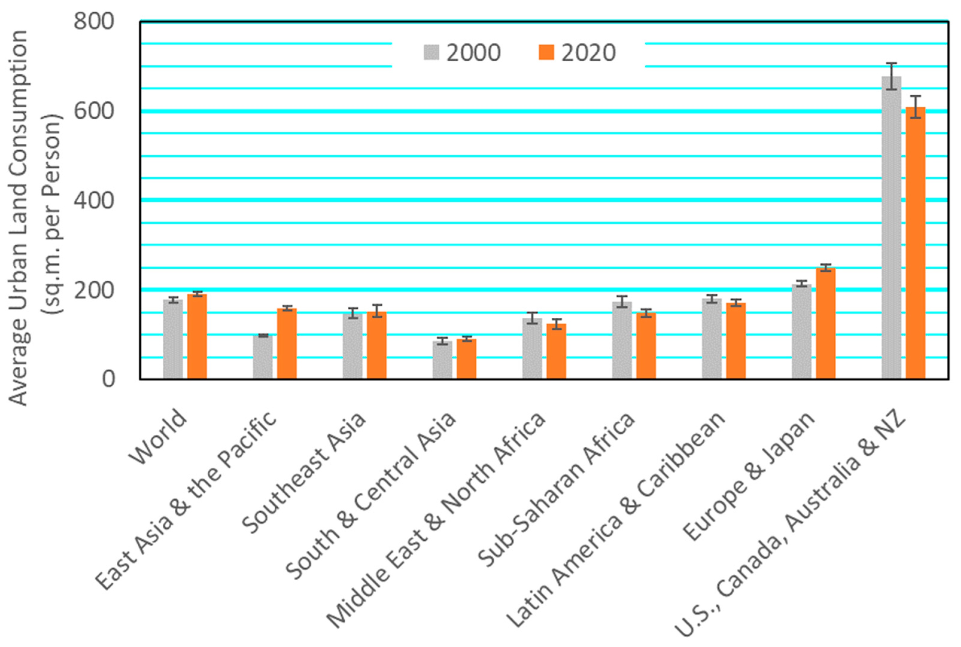
3.1. Regional Variations in Urban Land Consumption, 2000–2020

Given the focus on changes in urban land consumption in this article, it is important to put these changes in context by noting that there are large variations in the levels of urban land consumption—measured here in square meters of urban extent (rather than built-up area) per person—between different cities, countries, and regions. We focus here on variations in urban land consumption among world regions. These are illustrated in Figure 3. Average global urban land consumption was 178 square meters per person in 2000, which increased to 191 by 2020. The regions with the highest values for urban land consumption by far were the U.S., Canada, Australia, and New Zealand regions (667 in 2000 and 609 in 2020), followed by Europe and Japan (214 in 2000 and 250 in 2020). The region with the lowest values was the South and Central Asia region (85 in 2000 and 91 in 2020), followed by the Middle East and North Africa (137 in 2000 and 134 in 2020). Sub-Saharan Africa, although poorer, on average, than these two regions, had higher levels of urban land consumption (174 in 2000 and 149 in 2020). Among the regions in the Global South, Latin American and the Caribbean had the highest levels of urban land consumption (180 in 2000 and 171 in 2020).
When focusing on changes in urban land consumption, as we do here, it is important to keep in mind that in some cities and countries—Kinshasa in the Democratic Republic of Congo is one example—low levels of land consumption are associated with overcrowding [26]. The call for reducing urban land consumption in these cases may be inappropriate.

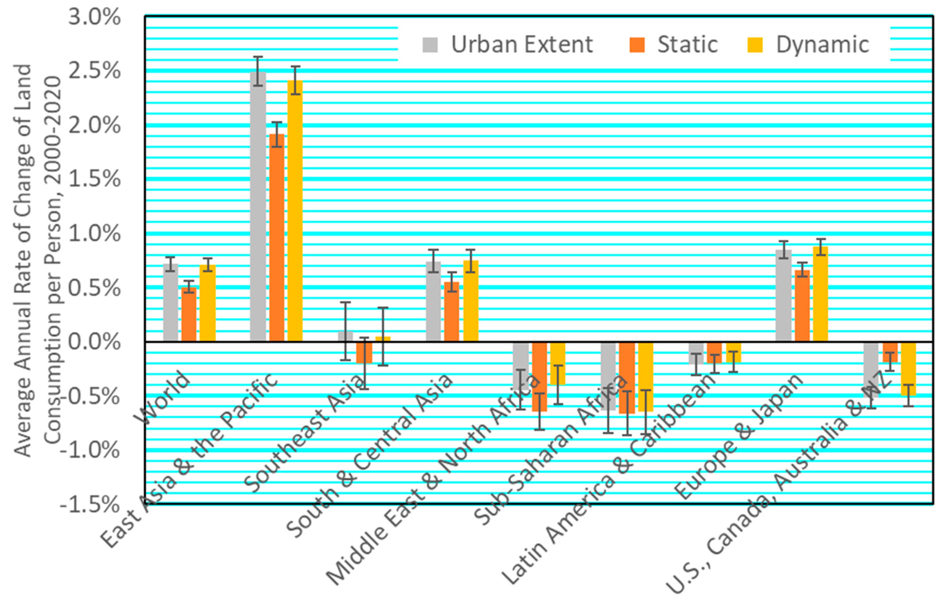
3.2. Regional Variations in the Land-Consumption-Change Indicators

The three land-consumption-change indicators introduced earlier can be calculated for each city from information on its population and area in 2000 and 2020. There is an issue, of course, of what is defined as the denominator, or the area, in the two periods. In this study, we used three methods to calculate this indicator, each using a different area in the denominator: (1) using the 2000 and 2020 urban extents of the city (which include built-up areas, urbanized open spaces, and roads), as we did in the previous section, in the denominator; (2) using the static method built-up area (the built-up area in 2000 within the 2020 extent and the built-up area in 2020 within the 2020 urban extent) in the denominator (as well as similarly calculating the population numerator for 2000 based on the 2020 extent); and (3) using the dynamic method built-up area (the built-up area in 2000 within the 2000 extent and the built-up area in 2020 within the 2020 urban extent) in the denominator. We introduced the urban extent method, a variation on the dynamic method, as an alternative approach that may more accurately represent the entire urban area of a city and its multiple land uses—including its urbanized open space—rather than just the built-up areas within that urban extent.
The results for all cities in our universe of cities for each of the three indicators and for each of the three methodological variations are categorized into eight world regions and the world at large, and their mean values and 95% confidence ranges are discussed below.
Using Indicator 11.3.1, we observed that the average value—using both the urban extent or the dynamic method built-up area—was significantly positive for the world at large (1.6 ± 0.8 for both) and for all world regions except Europe and Japan, where it was not different from 0, suggesting that global urban land consumption became less efficient during the 2000–2020 period. There was no significant difference in average values among the regions, except that average values for South and Central Asia were significantly higher than those for the Middle East, North Africa, and Sub-Saharan Africa. The error terms for the average values for the static method were large and, as a result, average values for the world at large and for all regions were not significantly different from zero, except for Sub-Saharan Africa (1.0 ± 0.2).
In contrast, the results for the average rates of annual land consumption per person, as an alternative to Indicator 11.3.1, were quite robust, as shown in Figure 4.
The figure shows that there were some significant differences in the results between the three methods of calculating the average rates in any single world region, but they were small compared to the significant differences between the world regions. These latter differences were due to the much smaller error terms in these measurements. In the world at large, the average annual rate of land consumption per person increased at an annual rate of 0.5–0.7%, depending on the way it was measured. The 95% errors were of the order of 0.06%, so we can conclude that the increase was statistically significant. The average rates declined significantly in three world regions and increased in four others. One region, Southeast Asia, showed nearly unchanged average rates, but with a mix of negative and positive density changes using the three methods for calculating the indicator. Significant rates of increase in the average annual rate of land consumption per person among world regions were observed in East Asia and the Pacific, Europe and Japan, and South and Central Asia. Significant rates of decline were present in Latin America and the Caribbean, Sub-Saharan Africa, the Middle East and North Africa, and the land-rich developed countries, where urban land consumption, overall, became more efficient.
It is also important to note that the values of this indicator were bounded, unlike the values for Indicator 11.3.1. No values observed were lower than −13% per annum or higher than 9% per annum, and several of the extreme values might be attributed to errors in the datasets.

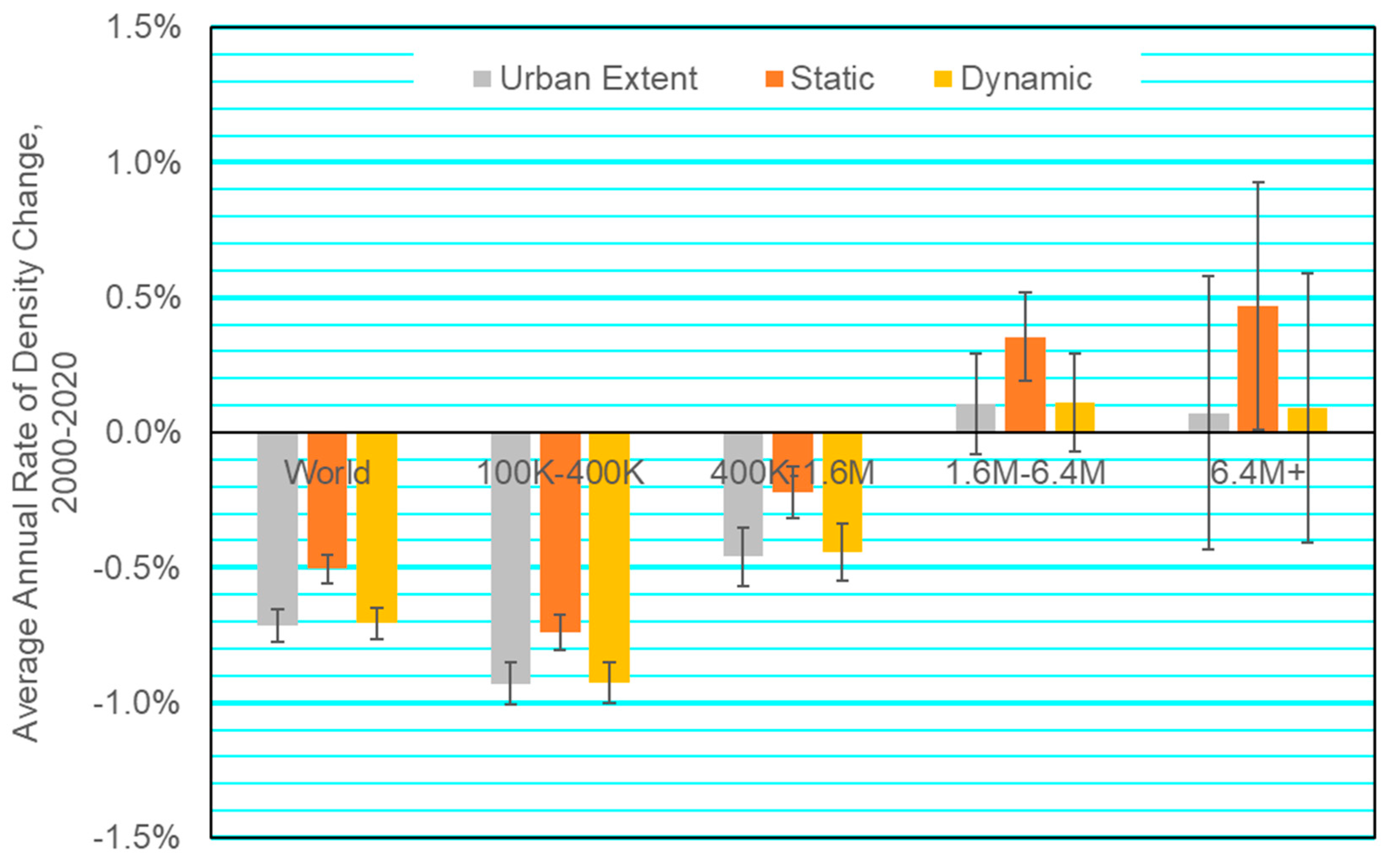
3.3. Variations in the Land-Consumption-Change Indicators among Cities of Different Sizes

It is worth noting that a graph for the average rate of change of density among the world regions is identical to the graph shown in Figure 4, except that where the rates of change for the land consumption per person indicator are positive, the rates for density change are negative, and vice versa. In this section, for a change, we focus on the average rate of density change in cities in different population size ranges.
To assess the variations between the land consumption indicators by city population size, we divided the cities into four population size ranges, given their 2020 populations as derived from our calculation from the GHS-POP dataset: (1) cities with 100,000–400,000 people; (2) cities with 400,000–1,600,000 people; (3) cities with 1,600,000–6,400,000 people; and (4) cities with more than 6,400,000 people.
Using Indicator 11.3.1, we could not observe systematic variations between cities in different population size ranges because their error terms all overlapped. The average rates of density change, however, did show some clearer patterns by city size range (Figure 5). While the error ranges in very large cities made comparisons to this group difficult, density decline was significantly faster, on average, in smaller cities than in larger ones. This suggests that small and intermediate cities were expanding less efficiently than large cities and megacities.

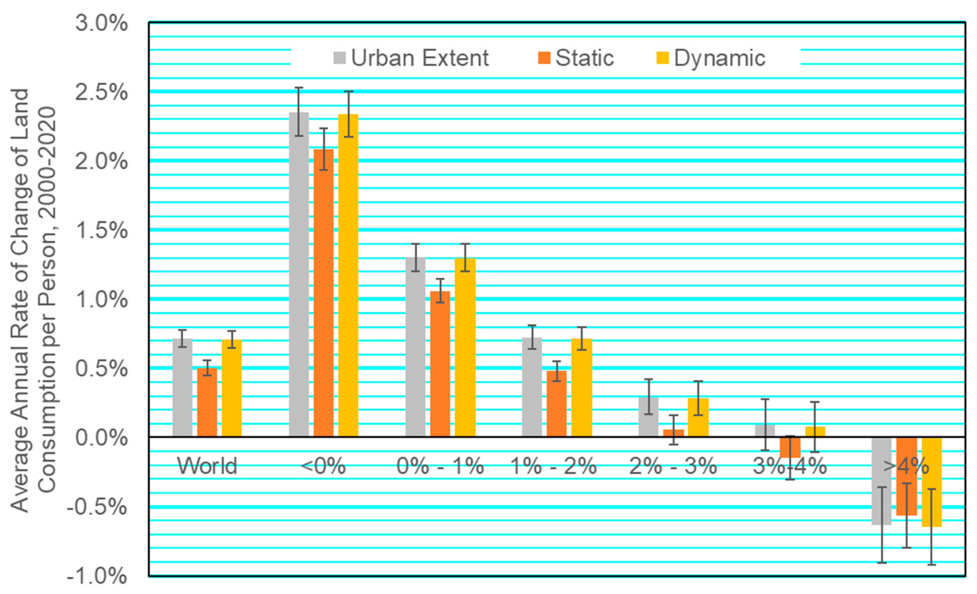
3.4. Variations in Land-Consumption-Change Indicators among Cities with Different Population Growth Rates

To assess variations between the indicators by city population growth rates, we divided the universe of cities into six categories, depending on their average dynamic annual population growth rate during the 2000–2020 period: (1) cities that had negative average growth rates; (2) cities with average growth rates between 0% and 1% per annum; (3) cities with growth rates between 1% and 2% per annum; (4) cities with growth rates between 2% and 3% per annum; (5) cities with growth rates between 3% and 4% per annum; and (6) cities with growth rates above 4% per annum.
It was difficult to interpret the results when they were measured by Indicator 11.3.1. There were significant differences, however, in the average annual rates of change in land consumption per person among cities in different population growth rate ranges (Figure 6). Generally, more rapidly growing cities experienced significantly lower rates of increase in land consumption per person. Cities that lost population, of course, had the highest increases in land consumption per person. In contrast, cities that grew in population at an average of 4% or more per annum experienced negative rates of growth of land consumption per person over the 2000–2020 period.

4. Discussion

Indicator 11.3.1—the metric measuring change in urban land consumption—has proved to be an important indicator for assessing progress on the UN Sustainable Development Goals (SDGs). The indicator in its present formulation, however, poses serious problems, both in its measurement and in its interpretation. The two metrics proposed here as alternative measures of the efficiency of land consumption in cities—the rate of change of land consumption per person and the rate of density change—overcome the inherent limitations of Indicator 11.3.1. Variations on the methods of measuring these indicators—static, dynamic, or urban extent—may be relevant for different applications. The initial results from the GHSL built-up and population datasets for a large subset of the universe of cities and metropolitan areas that had 100,000 people or more in 2020 show a mix of results. Land consumption became more efficient in some world regions and less efficient in others. Globally, land consumption has become less efficient, on average, as well as less efficient in smaller cities and more efficient in rapidly growing ones. For the time being, we have no theory or hypothesis that would explain these differences, and such questions are outside the scope of this study but are worthy of additional research. These statistical findings should not be interpreted as proposing a global or regional norm for policy purposes, as sustainable development needs are context specific and may call for higher or lower land consumption per capita than current levels. Relatedly, land consumption per capita is only one approach to conceptualize the “efficiency” of land use (indeed, there are even many additional dimensions of urban density alone [26]), and many other dimensions of the issue may need to be considered when planning for all pillars of sustainable development, but these other dimensions are outside the narrower focus of this research. These findings, for a single period only, also give us limited insights into the shifting trends over different periods, or over longer or shorter time scales, a shortcoming for future research to address. That said, we have demonstrated in this paper that the efficiency of land consumption can indeed be measured in a rigorous and precise way, and that there are global datasets now available for the 2000–2020 period and additional recent years that can be used to calculate the efficiency of land consumption in all cities and countries, and to draw some preliminary conclusions concerning variations among world regions, among cities in different size ranges, and among cities growing at different rates.

Supplementary Materials

The following supporting information can be downloaded at: https://www.mdpi.com/article/10.3390/land13091491/s1, Spreadsheet with population and area values and indicators calculated for each city included in assessment.

Author Contributions

Conceptualization, S.A. and E.M.; methodology, S.A. and E.M.; software, B.G.-W. and E.M.; validation, S.A. and E.M.; formal analysis, S.A., E.M. and B.G.-W.; investigation, S.A.; resources S.A., E.M. and B.G.-W.; data curation, E.M. and B.G.-W.; writing—original draft preparation, S.A. and E.M.; writing—review and editing, S.A. and E.M.; visualization, S.A.; supervision, S.A.; project administration, S.A.; and funding acquisition, S.A. and E.M. All authors have read and agreed to the published version of the manuscript.

Funding

WRI received funding from Steven M. Ross, the Patrick J. McGovern Foundation, and the Bezos Earth Fund, which supported this research.

Data Availability Statement

The original data presented in this study are openly available. The global urban extent boundaries are on the Google Earth Engine and accessible for analysis as feature collection assets for each year at ‘projects/wri-datalab/cities/urban_land_use/data/urban_extents/GHSL_BUthresh10pct_XXXX_V1’, where XXXX is the year of interest. Extents are available in 5- or 10-year intervals from 1980 to 2020. The scripts used to create the extents are at https://github.com/wri/urban_extent/releases/tag/v1 (accessed on 2 September 2024). The scripts for calculating the land consumption variables within each extent and the spreadsheets used for analyses of urban land consumption trends are available upon request.

Acknowledgments

We would like to thank Patrick Lamson-Hall for his contributions to earlier related research. Thanks to Google’s support through their Geo for Good Cloud Credits program. The 2016 Atlas of Urban Expansion was made possible by financial support from UN-Habitat, the Lincoln Institute of Land Policy, and the Marron Institute at New York University. Thanks to UN-Habitat for convening the Expert Group Meeting on Land Use and Urban Green Areas in December 2023, where an early version of this research was discussed. Thanks also to Dennis Mwaniki, Robert Ndugwa, and Lewis Dijkstra for their constructive comments during our presentation there.

Conflicts of Interest

The authors declare no conflicts of interest. The funders had no role in the design of the study; in the collection, analyses, or interpretation of data; in the writing of the manuscript; or in the decision to publish the results.

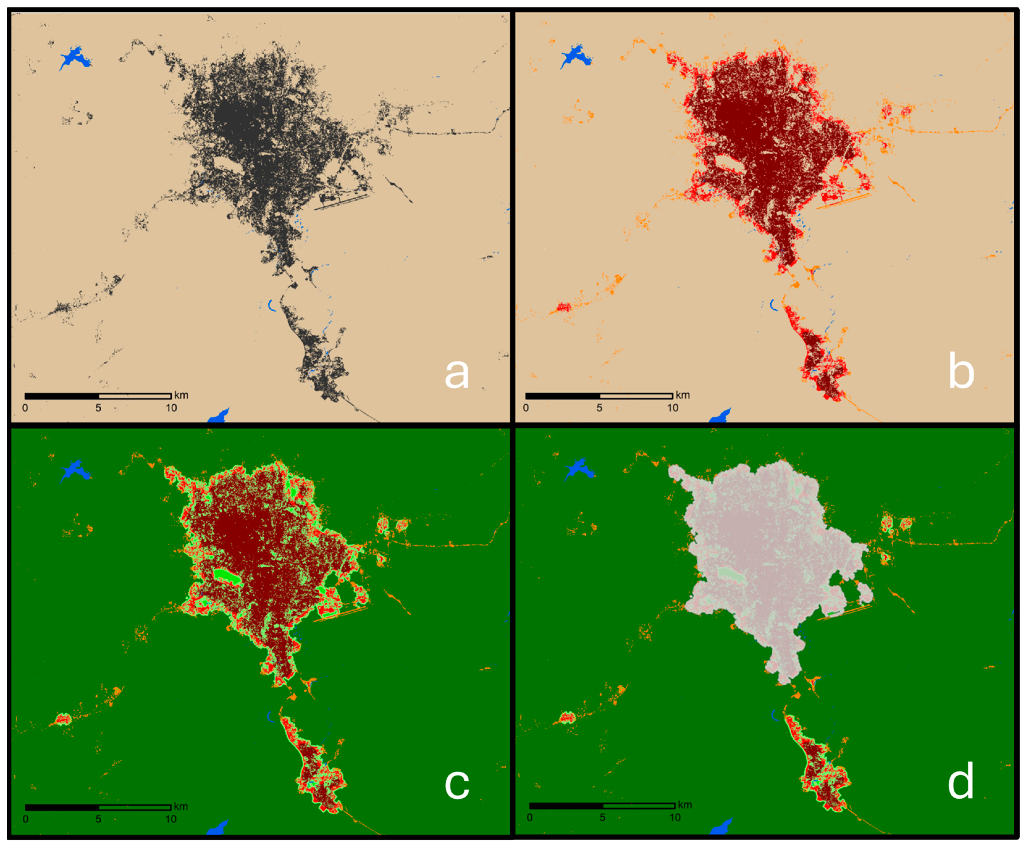
Appendix A. Methods to Delineate Urban Extents

In mapping the urban extents of all the cities in the universe, we followed the steps articulated here:
  • Obtain centroids for cities of interest and a built-up layer for their regions. For centroids, we used latitudes/longitudes of city central business districts available from the Atlas’s universe of cities. For built-up layers, we used GHS-BUILT-S R2023A at 100-m resolution, including only pixels classified as having 10% or greater built-up coverage, for years 1980 to 2020 at five-year intervals.
  • For each city i, define an overly inclusive maximum area of interest (the “study area”) using a radius (Ri) from city centroid based on the estimated city population (Pi) and slope (Sr) and intercept (Ir) from the linear average relationships between the population and built-up area for all cities in each world region r of the Atlas and scale it by 20 times.
    R i = e ( S r × ln P i + I r ) × 20 π
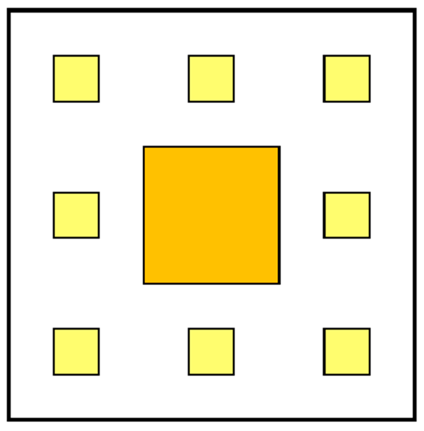
  • For each year, classify each built-up pixel within the area of interest based on the percent of pixels that are built-up within its 1 km2 circular neighborhood, an area with a radius roughly equivalent to a ten-minute walk. If 50% or more of the pixels in the circle are built-up, the pixel is classified as urban. If less than 50%, but 25% or more of the pixels in the circle are built-up, the pixel is classified as suburban. If less than 25% of the pixels in the circle are built-up, the pixel is classified as rural.
  • Vectorize all contiguous urban and suburban pixels to form urban cluster polygons.
  • Calculate the influence distance d of each urban cluster with an area A as the depth of a buffering ring around a circle with an area A and ring area equal to 0.25A.
    d = 1.25 A π A π = A · 0.06659
  • Buffer each urban cluster polygon by its influence distance d. Dissolve all buffered polygons to merge the polygons of those with overlapping influence areas. Retain only polygons that are within 200 m of the city centroid. Merge all remaining polygons into a single feature.
  • Mask classified built-up pixels from step 3 to retain only those within the feature polygon.
  • Filter urban and suburban pixels to retain only those within clusters (from step 4) that contain at least one urban pixel. Vectorize these urban and suburban pixels as a single feature.
  • Fill any holes within the feature polygon that are less than 200 ha in area. Include them in the feature polygon. This feature provides the urban extent.
  • Repeat for each city and year of interest.
Using the Google Earth Engine, we resampled all raster datasets to 100 m. For population data, we additionally scaled the pixel population counts to distribute the same aggregate counts across the pixels at the new resolution. We ran a sum reducer on each urban extent geometry for each year to determine the total population count and total area of built-up pixels within each extent. We also calculated the area of each urban extent. To enable calculations using both the static and dynamic methods, the totals for the year 2000 were calculated using both the 2000 extents and the 2020 extents.
The resulting dataset required some cleaning up. Of the original universe of 4231 cities dataset, we combined cities with contiguous footprints by 2020 to form 175 urban agglomerations. In addition, we removed several hundred cities that had less than 100,000 in population in 2020 according to our calculations based on the GHS-POP dataset. Because different methods were used to derive these population estimates than those that were used to derive the original Atlas universe population estimates, it makes sense that the population counts and number of cities above this threshold vary. This reduced the total number of cities to be analyzed further to 3470.

References

  1. UN Statistical Division. Global Indicator Framework for the Sustainable Development Goals and Targets of the 2030 Agenda for Sustainable Development; United Nations: New York, NY, USA, 2023. [Google Scholar]
  2. Burton, E. The Compact City and Social Justice. In Housing, Environment and Sustainability; University of York: York, UK, 2001; pp. 1–16. [Google Scholar]
  3. OECD. Compact City Policies: A Comparative Assessment; OECD Green Growth Studies; OECD Publishing: Paris, France, 2012. [Google Scholar]
  4. Camagni, R.; Gibelli, M.C.; Rigamonti, P. Urban mobility and urban form: The social and environmental costs of different patterns of urban expansion. Ecol. Econ. 2002, 40, 199–216. [Google Scholar] [CrossRef]
  5. Li, G.; Fang, C.; Li, Y.; Wang, Z.; Sun, S.; He, S.; Qi, W.; Bao, C.; Ma, H.; Fan, Y.; et al. Global impacts of future urban expansion on terrestrial vertebrate diversity. Nat. Commun. 2022, 13, 1628. [Google Scholar] [CrossRef] [PubMed]
  6. Dadashpoor, H.; Hasankhani, Z. Exploring patterns and consequences of land consumption in a coastal city-region. Ecol. Process. 2022, 11, 49. [Google Scholar] [CrossRef]
  7. Montejano, J.; Monkkonen, P.; Guerra, E.; Caudillo, C. The Costs and Benefits of Urban Expansion: Evidence from Mexico, 1990–2010; Lincoln Institute of Land Policy: Cambridge, MA, USA, 2019. [Google Scholar]
  8. Dijkstra, L.; Poelman, H. A Harmonised Definition of Cities and Rural Areas: The New Degree of Urbanization; Working Paper 01/2014; Directorate-General for Regional and Urban Policy, European Commission: Brussels, Belgium, 2014. [Google Scholar]
  9. Dijkstra, L.; Poelman, H.; Veneri, P. The EU-OECD Definition of a Functional Urban Area; OECD Regional Development Working Papers, No. 2019/11; OECD: Paris, France, 2019. [Google Scholar]
  10. Angel, S.; Blei, A.M.; Lamson-Hall, P.; Galarza, N.; Gopalan, P.; Kallergis, A.; Civco, D.L.; Kumar, S.; Madrid, M.; Shingade, S.; et al. Atlas of Urban Expansion, 2016th ed.; New York University: New York, NY, USA; UN-Habitat: Nairobi, Kenya; Lincoln Institute of Land Policy: Cambridge, MA, USA, 2016. [Google Scholar]
  11. Yang, Q.; Xu, Y.; Tong, X.; Hu, T.; Liu, Y.; Chakraborty, T.C.; Yao, R.; Xiao, C.; Chen, S.; Ma, Z. Influence of urban extent discrepancy on the estimation of surface urban heat island intensity: A global-scale assessment in 892 cities. J. Clean. Prod. 2023, 426, 139032. [Google Scholar] [CrossRef]
  12. Angel, S.; Lamson-Hall, P.; Guerra, B.; Liu, Y.; Galarza, N.; Blei, A.M. Our Not-So-Urban World; Working Paper No. 42; The Marron Institute of Urban Management: New York, NY, USA; New York University: New York, NY, USA, 2018. [Google Scholar]
  13. United Nations Human Settlements Programme. SDG Indicator Metadata, Indicator 11.3.1: Ratio of Land Consumption RATE to Population Growth Rate; United Nations: New York, NY, USA, 2021. [Google Scholar]
  14. Clark, C. Urban Population Densities. J. R. Stat. Soc. Ser. A (Gen.) 1951, 114, 490–496. [Google Scholar] [CrossRef]
  15. Alonso, W. Location and Land Use: Towards a General Theory of Land Rent; Harvard University Press: Cambridge, MA, USA, 1964. [Google Scholar]
  16. Schiavina, M.; Melchiorri, M.; Pesaresi, M.; Politis, P.; Carneiro Freire, S.M.; Maffenini, L.; Florio, P.; Ehrlich, D.; Goch, K.; Carioli, A.; et al. GHSL Data Package 2023; Publications Office of the European Union: Luxembourg, 2023; ISBN 978-92-68-02341-9. [Google Scholar]
  17. Marconcini, M.; Metz-Marconcini, A.; Üreyen, S.; Palacios-Lopez, D.; Hanke, W.; Bachofer, F.; Zeidler, J.; Esch, T.; Gorelick, N.; Kakarla, A.; et al. Outlining where humans live, the World Settlement Footprint 2015. Sci. Data 2020, 7, 242. [Google Scholar] [CrossRef] [PubMed]
  18. Gorelick, N.; Hancher, M.; Dixon, M.; Ilyushchenko, S.; Thau, D.; Moore, R. Google Earth Engine: Planetary-scale geospatial analysis for everyone. Remote Sens. Environ. 2017. [CrossRef]
  19. Sims, K.; Reith, A.; Bright, E.; McKee, J.; Rose, A. LandScan Global 2021 [Data Set]; Oak Ridge National Laboratory: Oak Ridge, TN, USA, 2022.
  20. Tatem, A. WorldPop, open data for spatial demography. Sci. Data 2017, 4, 170004. [Google Scholar] [CrossRef] [PubMed]
  21. Bonatz, H.; Reimann, L.; Vafeidis, A.T. Comparing built-up area datasets to assess urban exposure to coastal hazards in Europe. Sci. Data 2024, 11, 499. [Google Scholar] [CrossRef] [PubMed]
  22. Leyk, S.; Uhl, J.H.; Balk, D.; Jones, B. Assessing the accuracy of multi-temporal built-up land layers across rural-urban trajectories in the United States. Remote Sens. Environ. 2018, 204, 898–917. [Google Scholar] [CrossRef] [PubMed]
  23. MacManus, K.; Balk, D.; Engin, H.; McGranahan, G.; Inman, R. Estimating population and urban areas at risk of coastal hazards, 1990–2015: How data choices matter. Earth Syst. Sci. Data 2021, 13, 5747–5801. [Google Scholar] [CrossRef]
  24. Leyk, S.; Gaughan, A.E.; Adamo, S.B.; de Sherbinin, A.; Balk, D.; Freire, S.; Rose, A.; Stevens, F.R.; Blankespoor, B.; Frye, C.; et al. The spatial allocation of population: A review of large-scale gridded population data products and their fitness for use. Earth Syst. Sci. Data 2019, 11, 1385–1409. [Google Scholar] [CrossRef]
  25. Yin, X.; Li, P.; Feng, Z.; Yang, Y.; You, Z.; Xiao, C. Which Gridded Population Data Product Is Better? Evidences from Mainland Southeast Asia (MSEA). ISPRS Int. J. Geo-Inf. 2021, 10, 681. [Google Scholar] [CrossRef]
  26. Angel, S.; Lamson-Hall, P.; Gonzalez Blanco, Z. Anatomy of density: Measurable factors that constitute urban density. Build. Cities 2021, 2, 264–282. [Google Scholar] [CrossRef]
Figure 1. The Atlas of Urban Expansion method of obtaining an urban boundary for Addis Ababa, Ethiopia, in 1990. (a) Built-up pixels. (b) Pixels classified based on the built-up status of neighboring pixels. (c) Captured vs. rural open space pixels classified. (d) Urban extent area (transparent white).
Land 13 01491 g001
Figure 2. An abstraction of a city with its urban extent in 2000 (orange square), with eight settlements on its periphery that were already built in 2000 (yellow squares), and its urban extent in 2020 (outer square).
Land 13 01491 g002
Figure 3. Variation in urban land consumption among world regions during 2000–2020.
Land 13 01491 g003
Figure 4. Regional variations in the average annual rate of change of land consumption per person during the 2000–2020 period.
Land 13 01491 g004
Figure 5. Average annual rates of density change in cities in different population ranges during the 2000–2020 period.
Land 13 01491 g005
Figure 6. Average annual rates of change of land consumption per person in cities in different population growth ranges.
Land 13 01491 g006
Disclaimer/Publisher’s Note: The statements, opinions and data contained in all publications are solely those of the individual author(s) and contributor(s) and not of MDPI and/or the editor(s). MDPI and/or the editor(s) disclaim responsibility for any injury to people or property resulting from any ideas, methods, instructions or products referred to in the content.

