Abstract
The concept of segregation analyses the unequal distribution of social groups between neighbourhoods. It rests on two assumptions: that of homogeneous neighbourhoods and of a market liberal housing system. Both assumptions are applicable the context of American cities, but they display severe limitations when applied to the European context. Vienna’s housing market is particularly highly segmented, not only throughout the city as a whole but also within neighbourhoods. In the densely built-up area, residential buildings of different segments with different underlying rent regulations and entry barriers can be found side by side. Therefore, buildings are expected to show varying tenant and owner structures, which undermines the idea of a homogeneous neighbourhood. Against this background, we analyse at the micro scale small neighbourhoods defined by 100 m grid cells in a case study of two inner-city Viennese districts (districts 6 and 7) characterised by a particularly vivid housing-transformation and commodification dynamic. Using a novel and fine-grained dataset combining building information with the socio-economic data of households, we investigate the patterns and dynamics of income inequality and income segregation, as well as the relationship between housing market segments and socio-economic patterns. As data comprise two cross-sections for the years 2011 and 2020/21, changes in the neighbourhoods during the house-price boom period are also considered. This leads us to ask the question: How do housing market segmentation and its related changes affect income inequality and segregation at the micro scale? Our analysis delivers two main results: Firstly, we show the existence of marked social variation and related dynamics at the micro scale, even within a small urban area. Secondly, we show that the spatial distribution of housing market segments has a strong impact on income inequality in the neighbourhood.
1. Introduction
The concept of residential segregation, i.e., the spatial distance between different social groups or the spatial concentration of similar social groups, relies on two basic assumptions that have been observed by social scientists of the School of Chicago: firstly, the existence of socially homogeneous neighbourhoods (e.g., in terms of income, educational level, or race/cultural background), and secondly, a liberal housing market, where demand and supply drive the price gradient that determines the mobility of households in urban space [1]. Based on these assumptions, Burgess’s model of homogeneous zones in urban space and the mobility of new social groups between these zones has influenced our understanding of social patterns, segregation, household mobility, and neighbourhood change for almost a century [2].
These classical principles of residential segregation have been questioned by two strands of the literature: Firstly, the debate on micro-segregation, which analyses segregation within or between single residential buildings [3]. Although this debate has emerged in the last few years, micro-segregation is a historic phenomenon: residential buildings in 19th-century metropolises such as Vienna or Paris displayed a very pronounced vertical social differentiation [4,5]. Further, beyond the European city, neighbourhoods in southern cities in the United States likewise display a high degree of social variety at the scale of individual buildings [6,7]. Alongside the vertical expansion of the modern city after World War II, this issue increasingly arose in various cities [1,8]. The second strand addresses allocation mechanisms influencing the housing market: the existence of informal and non-market-based allocation [9], the interplay of market- and non-market-segments [10], or the degree of market segmentation [11] have implications for the residential segregation of the housing market. This is relevant insofar as housing market segments differ regarding their accessibility and entry barriers for households [12]. Consequently, the spatial distribution of housing market segments in the city can either drive or cushion income inequality and, as a consequence, income segregation at various spatial scales.
The main intention of this paper is twofold: Firstly, it analyses the relevance and magnitude of micro-scale income segregation, using income inequality as its prerequisite, for two inner-city districts in Vienna. Secondly, it estimates the impact of housing market segmentation on inequality and segregation against the backdrop of Vienna’s housing boom during the 2010s. For this purpose, we link a dataset outlining housing market segmentation at the scale of individual residential buildings with various socio-economic register data at the scale of households, provided by the Austrian Micro Data Centre (AMDC) [13]. Based on this database, and by applying separate multiple linear regression models, we investigate the relationship between the dependent variables of income, inequality, and segregation and a set of predictor variables including housing market segmentation. The analysis is conducted for 2011 and 2020/21, at the scale of a 100 × 100 metre grid, focusing on a case study in Vienna’s high-density built-up area (districts 6 and 7).
Vienna is a useful case study for the analysis of the relevance of micro-segregation and the role of market segmentation for two reasons. Firstly, Vienna’s housing market displays a high degree of market segmentation, in particular in comparison to most other larger metropolises. Secondly, Vienna’s housing market has experienced an enormous house-price boom during the last 15 years, which, on one hand, triggered a construction boom in the large urban expansion areas at the periphery [14]. On the other hand, this boom gave rise to the commodification of the existing housing stock, with greatly varying implications for the housing market segments. Against this background, our analysis investigates the patterns and drivers of micro-segregation in a study area characterised by a high share of historic housing stock in a period of a booming housing market.
This paper is structured as follows: In Section 2, we discuss the interplay between the scalarity of segregation and housing market segmentation, provide an overview of the segmentation and dynamic of Vienna’s housing market, and formulate the research question. Following the description of the materials and methods used and a presentation of the research area (Section 3), we discuss our results in Section 4, covering the patterns and dynamics of income inequality and residential segregation and the role of housing market segmentation in that regard. In Section 5, we discuss our results, their limitations, and their further conceptual implications and provide a conclusion (Section 6).
2. Research Context: Micro-Segregation and Housing Segmentation
Segregation can be defined as the formation of distinct patterns of over- and under-representation of specific social groups across residential space [1]. The classic literature based on the socio-ecological model of the Chicago school relies on two assumptions: Firstly, the existence of homogeneous neighbourhoods, which allows the measurement of segregation between statistical units. Secondly, a liberal housing market, where social differentiation in urban space is driven by households that compete on account of their incomes to realise their housing preferences [15]. In the following section, we scrutinise both assumptions, particularly for the European city.
2.1. The Micro Scale: Vertical and Horizontal Segregation
The recent debate on micro-segregation points to social inequality at the scale of individual buildings within a neighbourhood [3,8]. Besides some examples from historic case studies in cities in the Southern USA, micro-segregation is de facto discussed synonymously with vertical segregation. As such, vertical segregation means micro-segregation within residential buildings, while horizontal micro-segregation describes socio-economic differences between them.
Segregation within individual buildings has a long history. The residential buildings of the Belle Époque particularly displayed pronounced social differentiation: from the bourgeois Belle Étage, holding the highest social status, a declining social gradient led towards the poorest households, situated in the last storey, directly under the roof [5]. During the twentieth century, emerging from cities in the USA, the verticalisation of the urban fabric became a global phenomenon [16]. As such, the vertical differentiation of urban society presents itself in various forms: rooftop extensions in the existing housing stock of European metropolises such as Paris or Vienna [17], social differentiation in former socialist housing estates in Eastern Europe [18], or high-rise buildings as a dominant building type, with a strong degree of vertical segregation within the building and/or its surroundings—for instance, in Santiago de Chile [19] or Hong Kong [20]. These cases of micro-segregation all share the dimension of vertical social differentiation within a residential building.
In Europe, the phenomenon of vertical micro-segregation is much more widespread in cities in the south than in the north or west. This is a consequence of a specific built-up structure (prevalence of apartment buildings), the structure of the housing market (dominance of owner-occupation), and the specific context of housing provision [21]. Qualitative analyses for Athens reveal the long-term transformation of these condominium buildings, which show strong segregation between native Greek and migrant residents, between social groups, and, finally, between owners and tenants [22]. Similar patterns have been analysed for residential buildings in arrival spaces in Marseille [23] or for inner-city neighbourhoods in Naples [24].
Although vertical segregation is described as a sub-form of micro-segregation and social diversity is a core feature of the European city, there is hardly any research on horizontal micro-segregation [25]. Likewise, certain 19th-century cities in the USA featured a high degree of horizontal segregation at the micro scale. Logan and Bellman [6], for instance, identified different forms of ethnic segregation in Philadelphia between 1880 and 1900, where ‘black’ residential buildings in ‘white’ neighbourhoods were hidden in backyards or smaller, isolated back streets. This pattern was the outcome of a strategy to ensure social distance and control, as well as the availability of a (slave-)workforce within spatial proximity [26]. However, most segregation studies rather focus on statistical aggregates at the scale of statistical units or neighbourhoods, which hides the patterns and dynamics of socio-spatial inequality, as well as the mechanisms that lie behind them.
2.2. Residential Segregation and Housing Market Segmentation
The term ‘residential segregation’ implicitly points to the role of urban residents. Consequently, the housing market and its allocation system have an impact on urban segregation. As such, the housing market functions as an interface between the two dimensions of societal structures and dynamics, on the one hand, and spatial urban patterns, on the other hand.
In the classic literature that is based on the socio-ecological model of the Chicago school, the social differentiation of households in the urban space is driven by a liberal housing market [15]. Accordingly, the demands and preferences of different social groups within an existing price gradient determine the social pattern, as well as its dynamic, as the mobility of groups modifies the urban price landscape and shifts the borders between different social neighbourhoods, as explained in the arbitrage model [27]. In this liberal market model, residential income segregation relies on the presence of income inequality and “income-correlated residential preferences, an income-based housing market, and/or housing policies that link income to residential location” [28] (p. 1102). Thus, in a liberal housing market, income sorting and related segregation is driven by market preferences related to location factors, e.g., the distance from the city centre or quality of public spaces [29], or urban amenities such as education facilities [30], urban green [31], and metro stations [32]. As such, the price differential between the top- and bottom-quality/price submarket drives the market structure and its variation.
This assumption of a homogeneous urban housing market is questioned by the concept of housing market segments. Segments are defined by a variety of market mechanisms, regulations, allocation systems, and entry barriers. In a simple way, the segmentation of housing markets can be analysed by distinguishing between a rental and an ownership market. Here, Allen et al. [33] distinguish between ‘dual’ and ‘unitary’ housing systems, whereby the former is highly segmented between socially weak households that are concentrated in the rental segment and wealthy households on the ownership market. In the unitary housing system, in contrast, there is no social differentiation between the rental and ownership markets. A further division is provided by Kemeny [34], who distinguishes between an ‘integrated’ and a ‘dual’ rental system. In the integrated system, social housing provides good housing standards, competing directly with the private segment. In dual rental systems, on the other hand, social housing is restricted to households in need, which causes stronger social segmentation within the private rental sector.
As housing market segments rely on different legal regulations, they are characterised by different housing costs, and they display different entry barriers and access restrictions regarding social or ethnic groups. This implies an uneven distribution between market segments, also called ‘socio-tenure differentiation’ [12]. Consequently, it could be assumed that these segments are characterised by different resident structures with regard to different factors, e.g., household income, level of education, or migration background. As such, the access to different housing market segments plays a crucial role as a driver of the spatial (un)evenness of an urban population [35].
As the national and regional regulative context (tenancy law and welfare system), housing policy, and planning system are closely related to the differentiation of housing market segments, the consideration of these factors is crucial for the understanding of segregation [36,37], in particular in comparative urban research. For instance, Murie and Musterd [38] identified the social housing sector as relevant for explaining the different levels of segregation in Dutch and British cities. Kesteloot and Cortie [39] explained variations in ethnic segregation between Brussels and Amsterdam, and Skifter Andersen et al. [11] analysed the impact of social housing and urban policies on the level of ethnic segregation in different Nordic capitals. Thus, even if two cities display the same level of aggregate social inequality, the segmentation of the housing markets and their regulative context, in combination with spatial patterns within the urban space, might produce a different outcome regarding residential segregation at different scales.
2.3. Segmentation and Segregation on Vienna’s Housing Market
Vienna’s housing market displays a high degree of market segmentation: it comprises two segments of social housing, communal housing and limited-profit housing associations (LPHAs) [40], which together comprise about 42% of households in Vienna. Beyond that, a huge historic housing stock built pre-1945, with the vast majority of buildings being constructed during the ‘founders’ period‘ (1848–1918, ‘Gründerzeit’), comprises about 22% of the total stock in Vienna. This segment is socially relevant, because it is regulated by a law of tenancy (Mietrechtsgesetz, MRG), keeping its capped rental rates below the market level. Due to a combination of regulated, affordable rent prices and private, low-threshold access to housing, the historic housing stock often provides the first entry point to the housing market in Vienna for migrants [41]. In contrast, apartment buildings constructed after 1944 (11%) underlie a different tenure law, where rents are non-regulated. Beyond this, ownership housing makes up just about 20% [42].
Since the mid-2000s, the Viennese housing market has faced an enormous price boom, which triggered the transformation of the historic housing stock (by tenure conversion or demolishing/new construction) due to the increasing ‘value gap’ [43]. The outcome of this process is, on one hand, the changing social structure of residents, and on the other hand, increasing granularity between the housing market segments, in particular between the transformed and the non-transformed historic housing stock. Consequently, within one street block containing about 20 apartment buildings, we can find an increasing variety of housing market segments, representing different social structures and different means of access and mechanisms of exclusion; transformed and non-transformed residential buildings, as well as newly constructed residential buildings, are the drivers of this granularity.
For the case of Vienna, several authors point to the role of market segmentation and the specific housing market barriers regarding segregation: according to Giffinger [44], the accessibility of housing market segments drove the ethnic segregation of Turkish and ex-Yugoslavian immigrants in the 1990s. Hatz et al. [45] found that Vienna’s social geography had become more polarised in the early 2000s due to structural shifts in the economy, a neoliberal trend for stronger market-orientation in the housing sector, and spatially selective gentrification processes. More recently, Premov and Schnetzer [46] estimated the impact of the spatial prevalence of the council housing segment on local income inequality, confirming a positive relationship between the broad provision of council housing and the social mix within the neighbourhood. Kadi et al. [47] demonstrate that socio-spatial inequality in Vienna has increased, partly related to uneven housing market development since the financial crisis, driven by the private sector. Morawetz and Klaiber [32] demonstrate that the provision of municipality housing and capped rents moderate the income- and preference-based sorting of residents.
2.4. Housing Market Segmentation in Vienna—A Driver or Obstacle of (Micro-)Segregation?
The combination of a highly segmented housing market in Vienna and the increasing granularity of the spatial structure of these segments—in particular in the more central, inner districts—has implications for the measurement of residential inequality and segregation. The analysis at the scale of differently sized, politically or historically defined spatial units (e.g., census districts) hides the existing pattern of market segmentation and, therefore, its social implications, in particular regarding segregation dynamics between individual buildings. Consequently, we investigate the impact of housing market segmentation on income inequality between households existing in close proximity to each other (100 × 100 m cell grid), as well as the segregation of income groups in so-defined neighbourhoods compared to the overall distribution of income groups in the study area. Micro-scale variations in these phenomena are likely insofar as residential buildings in Vienna’s densely built-up area display pronounced variation regarding housing market segmentation (see Section 2.3). Two cross-sections for the years 2011 and 2020/21 were chosen to analyse the dynamics of the phenomena under consideration. This period includes two census years for which detailed register-based microdata are available, and it covers Vienna’s house-price boom, which started in the aftermath of the global financial and sovereign debt crisis of 2008–2010.
Building on existing research, we expect the spatial pattern of housing market segments to influence the level of income variation and residential segregation at the micro scale. In case of a boom of increasing house prices, similar to what we have experienced in Vienna during the last 15 years, we would expect increasing price differentiation within urban space, as price booms drive spatial variation in housing prices [48]. This would further imply increasing residential segregation, following a socio-spatial gradient from the city centre to the periphery. However, considering the high segmentation of Vienna’s housing market, this central–peripheral pattern would be distorted by the uneven distribution of the housing market segments, as the ability to pay is not the only allocation mechanism influencing Vienna’s housing market. Against this background, we can formulate the following research questions:
- (1)
- What are the spatial patterns and the dynamics of income inequality and segregation in the research area?
- (2)
- What is the effect of housing market segmentation in the neighbourhood on income inequality and segregation at the micro scale? How does this relationship change during the period 2011–2020/21?
3. Data, Methods, and the Research Area
3.1. Data
In this paper, we analysed the variation in household income in small neighbourhoods to quantify social inequality and residential micro-segregation. Even though strongly correlated to other variables of socio-economic status that have been used in segregation studies, such as occupational groups or educational attainment [49], this indicator had advantages over measures of segregation based on ordered or unordered categorical data. In particular, we did not lose information on the income distribution within and across spatial units, we were not influenced by arbitrary cut points to define groups (e.g., of income), and we did not limit the analysis to specific subgroups in society [28].
Our analysis was based on the Austrian wage-tax statistics (LUE) for 2011 and 2020 and labour market statistics (AEST) for 2011 and 2021, with socio-economic data on individuals obtained from the AMDC. For each individual, the data contained unique and pseudonymised keys attributing them to a household, building, and 100 × 100 m grid cell. To safeguard the robustness of inequality and segregation measures calculated by grid cell, cells with fewer than 30 households were excluded from the analysis. Data on building locations and attributes were taken from a geocoded dataset from the Austrian Address and Building Register (AGWR) and combined with building and address data from the Federal Office of Metrology and Surveying (BEV). Due to data gaps regarding the matching of the resident register and the AGWR, and due to the exclusion of certain grid cells for reasons of data protection, our dataset covered roughly 70% of persons and 90% of private households in our study area, which is still high compared to survey data [45,50].
However, certain methodological and conceptual issues related to income used in this study must be pointed out, as segregation measured by microdata can be very sensitive to the presence of measurement error and extreme values. The original data of gross yearly personal income including transfers (excluding capital income) received from the AMDC, on the one hand, contained some negative or very low values due to negative or very low taxable income (e.g., losses from self-employment, social security withholding, or inter-household mandatory payments). Some of these households might have been as well off as, or even better off than, other households in terms of material well-being, as they could draw on other sources of income not captured by wage tax statistics to cover their monthly expenses [51,52]. On the other hand, certain individuals had extremely high incomes. The related right skew of our income data reflects empirical evidence on the dispersion of the upper half of the income distribution. The literature suggests that this ‘upper-tail inequality’ has driven the growth in income inequality in the past few decades [53]. However, conceptually and related to our research question, with growing income or assets, the influence of housing affordability on the choice of residence—steered by housing policies and the supply of housing segments with capped rents, among others—decreases in relation to other factors of income- and preference-based sorting, such as proximity to amenities or distance to the city centre [32,54].
To improve the data structure and for the conceptual reasons mentioned above, negative and very low income values of individuals were bottom-coded by setting them to a 1000 EUR yearly income, and extreme values at the top end of the distribution were top-coded by setting them to 100,000 EUR yearly income. The winsorising of extreme values roughly concerned data below the 5th percentile and above the 95th percentile for both years. Further, as households—and not individuals— sort into buildings and apartments, we calculated equivalised household income based on the gross yearly incomes of all household members, including transfers. The aggregated household income was adjusted for household size by dividing the sum of individual incomes by the square root of the household size [55]. The equivalisation of household income allowed us to account for economies of scale in consumption and living costs and to control for intra-household inequality. To arrive at a set of socio-economic control variables at the household level, we took the employment status, educational attainment, and migration background of the highest earner (‘household reference person’) to be representative of the whole household.
The descriptive statistics presented in Table 1 provide summary statistics for the two cross-sections of 2011 and 2020/211. The sample comprised 28,101 (2011) and 29,620 (2020/21) households living in 272 grid cells in the sixth and seventh districts of Vienna. As dependent variables for each grid cell, our dataset contained the median annual gross equivalised household income, a bias-corrected Gini coefficient [56] measuring income inequality, and bootstrapped multi-group local segregation scores of the Mutual Information Index M [57] as a measure for segregation between income quintile groups. Median equivalised household income ranged between 11,430 EUR in the poorest and 63,210 EUR in the richest raster cell in 2011, increasing to a range of 10,460 EUR to 76,720 EUR in 2020. Regarding income inequality, the spread in the Gini coefficient of grid cells increased in this period, while the average coefficient stayed constant. Due to the top- and bottom-coding of outliers at the individual level, the originally strong right skew of the income variable at the household and grid-cell level was reduced. Lastly, segregation, as measured by local segregation scores, was characterised by a high variance distribution, with a coefficient of variation greater than 1. That is, income groups were rather homogeneously distributed across the majority of grid cells, which resulted in segregation scores close to zero in those grid cells.

Table 1.
Descriptive statistics of the datasets for 2011 and 2020/21. N = 272, 100 × 100 m grid cells.
The main explanatory variables of interest—the percentage share of households living in different housing market segments by grid cell—were constructed following a sequence of steps. In the first step, each building in the study area was attributed to a housing market segment by using a combination of sources [42]. In the second step, the number of households per building was calculated by matching each household with the unique building ID (AGWR OBJNR) obtained from the AMDC. Finally, the share of households living in different housing market segments by grid cell was calculated by spatially joining the geolocation of buildings and grid cells and aggregating the number of households per building belonging to a specific segment.
A set of demographic and labour market indicators hypothesised to have a strong effect on income variation within a grid cell were tested as control variables. All of these were calculated from individual-level statistics matched with households and buildings. Lastly, average property prices per square metre, sourced from DataScience Service GmbH, Wien, Austria, were included to control for price effects. This spatially detailed dataset is based on comprehensive geo-referenced broker data and sales contracts.
3.2. Methodology
We assessed the relationship of income, inequality, and segregation with housing market segmentation, while controlling for socio-economic status, agglomeration, and location effects, in three separate multiple regression models. Each model was run for the two cross-sections of 2011 and 2020/21. To arrive at the main dependent variables of interest for this study, inequality and segregation indices were computed by 100 × 100 m grid cells, based on equivalised household incomes, using R statistical software version 4.4.1 [58]. As a measure of income inequality between 0 (no concentration of income and, therefore, perfect equality) and 1 (maximum inequality), the Gini index was calculated with the R package ‘DescTools’ [59]. The data inputs for the calculation of the Gini index were household-level income data, grouped by spatial units. The resulting values depicted the degree of income inequality between households of a spatial unit and, therefore, inequality within neighbourhoods. As a measure of local income segregation, multi-group local segregation scores of the Mutual Information Index M2 were computed with the R package ‘segregation’ [60]. Local segregation scores of the entropy-based M index indicated the contribution of spatial units to the overall segregation of income groups in the study area and, therefore, inequality between neighbourhoods. The data inputs for the calculation of the segregation index were population counts per income groups (quintiles), grouped by spatial units. As we were working with very small neighbourhoods, we used the bootstrap function and bias correction built in the ‘segregation’ R package. However, 95% confidence intervals showed that local segregation scores were quite variable and, therefore, had to be interpreted conservatively.
With the calculation of inequality and segregation indices at the granular level of 100 × 100 m grid cells, we aimed to uncover the micro-scale neighbourhood sorting of households by income, which contributes in sometimes contradictory ways to large-scale patterns of inequality and segregation [28]. Grid cells represent a consistent definition of neighbourhood size and shape as opposed to historically or politically delineated units, which vary widely in their meaning across time and place. The three dependent variables were subjected to separate multiple regression analyses for 2011 and 2020/21, using ordinary least squares (OLSs). Based on a row-standardised queen contiguity spatial weights matrix, Moran’s I test for spatial dependence detected no spatial autocorrelation in the residuals of our models. Therefore, it was confirmed that OLS estimates were the most efficient solution as opposed to spatial regression models. However, the Breusch–Pagan tests indicated heteroscedasticity in the error terms, which is why we reported heteroscedasticity-robust confidence intervals in all regression results. Further, the variables ‘median household income’ and ‘Gini coefficient’ were log transformed to fit the structure of the data better and reduce potential bias in the results caused by outliers. The correlation matrix of variables tested and/or finally included in the regression models are presented in Appendix A.
The first empirical model, with the dependent variable representing the natural logarithm of the median household income in grid cell , has the following form:
where is the median equivalised household income for grid cell , is the constant or intercept term, and is a vector of variables representing the share of households encountered in four different housing market segments. The weight of housing provided by limited-profit housing associations (LPHAs) was used as reference group in the regression analysis. Further, denotes a vector of measures of the share of household reference persons by employment status, which has a direct relation to incomes. is a vector of variables representing household education levels. Furthermore, a vector of variables denoted by represents the share of persons born in ex-Yugoslavia, Turkey, Eastern EU/New Member States, and outside of Europe (i.e., first generation) and/or holding the citizenship of their respective birth countries (thus also including the second generation) as opposed to persons born in Austria and holding Austrian citizenship (i.e., no migration background). by grid cell represents average household size, the ratio of dependent persons (i.e., persons earning below 1000 EUR per year), and population density to control for the accumulation effect of personal income in households with multiple employed persons, as well as to control for agglomeration effects positively influencing wages, house prices, rents, service access, and the efficiency of public services [61]. in grid cells is included as a variable representing the share of households relocating within or from/to the area in the period 2011–2020/21. Theoretically, the residential mobility of households of different socio-economic statuses affects the distribution of top and bottom socio-economic groups in the neighbourhoods [62]. Lastly, represents a vector of indicators representing the quality of the neighbourhood—proxied by an ‘active mobility score’, ‘access to medium- and high centrality amenities’, and property prices—and the distance to the city centre as a proxy for agglomeration effects [32]. represents the idiosyncratic error term.
Model 2 is an extension of Model 1, where the natural logarithm of the Gini coefficient of household income in grid cell becomes the new dependent variable, and is added as a control variable to the right-hand side of the model. This is to control for the hypothesised large influence of the upper tail dispersion of the income distribution on the inequality measure. Model 3 is an extension of Model 2, where the of grid cell becomes the new dependent variable and the is added as a control variable to the right-hand side of the model. Due to the fact that the M index measures deviations from the global average in both directions (i.e., both, the over- or under-representation of certain income groups in a neighbourhood lead to a high local segregation score), the relationship between income and local segregation takes a U-shape rather than a linear one. Therefore, the variable is added to the model as a second-order polynomial (quadratic) term.
3.3. Study Area
The present study analysed an area comprising two inner-city districts of Vienna (district 6, Mariahilf, toward the south of the area under scrutiny, and district 7, Neubau, in the north). The study area is characterised by a very high building density, delimited by three high-level roads. The Belt Road (‘Gürtel’) defines the western boundary, Linke Wienzeile the southern boundary, and the so-called ‘Zweierlinie’, running parallel to the Ring Road, the eastern boundary. The northern district boundary is not characterised by as strong a morphological break as the others. Mariahilfer Straße—a well-known shopping promenade—cuts right through the middle of the study area (see Figure 1).
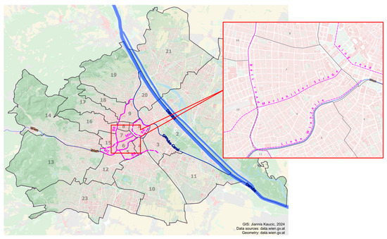
Figure 1.
The location of the study area within the city of Vienna. Note: BR = Belt Road; MH = Mariahilfer Straße; RR = Ring Road; WZ = Linke Wienzeile. Numbers denote the 23 Viennese districts.
During the last few decades, both districts have undergone intensive transformation: this is more apparent in the district Neubau, where the former middle- and working-class area was turned into a new urban creative milieu with a high share of academics [63]. The symbolic manifestations of gentrification are apparent in this district, in particular in the ground-floor zones, which are dominated by creative and alternative shops and restaurants. In comparison, the process of social upgrading has also affected the sixth district, Mariahilf, albeit to a lesser extent. Both districts exhibit a falling socio-economic gradient from the inner city (alongside the Ring Road) towards the peripheral zones (towards the Belt Road), but this is more apparent in Mariahilf. Compared to the city as a whole, both districts display an above-average resident income profile (Vienna: 24,400 Euro/head; Mariahilf: 25,700 Euro/head; Neubau: 27,200 Euro/head [64]).
4. Results
In the first subsection (Section 4.1), we analyse the detailed spatial patterns of household income levels, income inequality, and income segregation at the scale of grid cells. In the second subsection (Section 4.2), we intersect these patterns with the housing market segments and investigate the impacts of the different segments on the existing patterns while discussing changes between 2011 and 2020/21.
4.1. Spatial Patterns and Dynamics of Income Inequality and Segregation at the Micro Scale
What are the general patterns and dynamics of income inequality and segregation emerging from the spatial distribution of households with different income levels? Theil’s information theory index H [65]3, for income percentiles in 2011 and 2020, provides an initial insight into composite income segregation across micro-scale spatial units in the study area. Figure 2 indicates estimated segregation at the scale of 100 m × 100 m grid cells, between households with incomes above, at, or below each percentile of the study-area-wide household income distribution. As the H index is normalised between 0 and 1, the level of segregation of percentiles can be interpreted as percentages. The J-shaped segregation profile shows a tendency towards a larger spatial segregation of affluence (the extent to which the highest-income households are isolated from middle- and lower-income households), compared to segregation of poverty (the uneven distribution of low-income households among grid cells). Interestingly, segregation slightly decreased in the sixth and seventh districts of Vienna between 2011 and 2020. Generally, the entropy-based measurement of income segregation seems to be at a similar level to those of other urban areas (e.g., Beaubrun-Diant and Maury [66] or OECD [67]).

Figure 2.
Household income segregation for 2011 and 2020 across 100 × 100 m grid cells by income percentile, as measured by the information theory index H.
We now continue to explore the spatial patterns of median income levels, income inequality, and income segregation at the micro scale, comparing patterns across years. Figure 3 shows each variable in 100 × 100 m grid cells in separate maps for 2011 (left) and 2020 (right). For each variable individually, the range of attribute values was divided into five equal-sized sub-ranges and mapped to a colour scale to highlight the amount of an attribute value relative to other values. The legend gives an indication of the value distribution of each variable. The mapping of median equivalised household income as an indicator of socio-economic status within small neighbourhoods at the same time shows spatial patterns of inequality between these spatial units (Figure 3a,b). The spatial distribution shows a slight central–peripheral pattern and the clustering of cells with similar income levels in specific areas. Grid cells along and close to Mariahilfer Straße in the centre of the area, as well as in the areas closer to the city centre, belong to the more affluent group of neighbourhoods. In contrast, grid cells in the west of the study area along the Belt Road (‘Gürtel’), which has a high traffic load, as well as along the peripheral part of Linke Wienzeile (south-western part of the map), belong to the less affluent parts of the area. Furthermore, the central–peripheral pattern of income is overlayed by a dispersed, spatially random juxtaposition of grid cells with different income levels. Comparing spatial patterns between 2011 and 2020, we can observe the slight relative socio-economic status upgrading of some grid cells near neighbourhoods with already high socio-economic status, especially around Mariahilfer Straße. Apart from this, the spatial patterns of income levels remain stable between 2011 and 2020, meaning that the spatial clustering and central–peripheral gradient of income do not change significantly in the area.

Figure 3.
Spatial distribution of indices for 2011 (left) and 2020 (right) in 100 × 100 m grid cells. Panels (a,b) contain the median equivalised household income, panels (c,d) show the Gini coefficient of average equivalised household income, and panels (e,f) present the local segregation scores of the multi-group Mutual Information segregation index M of the equivalised household income quintiles.
The spatial patterns of income inequality within grid cells, measured by the Gini coefficient of equivalised household income (Figure 3c,d), show only a weak coincidence with the distribution of median income across grid cells in 2011, as well as a moderate negative one in 2020 (see correlation matrix in Appendix A). Due to the top- and bottom-coding of outliers and the use of median instead of mean income, there are only very few grid cells in which higher income levels also exhibit higher levels of income inequality. Mostly, we see evidence of a pattern of more affluent grid cells, e.g., along Mariahilfer Straße, that exhibit a lower income spread. In 2020—as also evidenced by the increasingly negative correlation coefficient—this pattern intensified, and income inequality further decreased in grid cells with higher income levels. This is likely due to the influx of households with similar income levels into these already affluent neighbourhoods. At the same time, some grid cells with lower income levels—along the Belt Road and Linke Wienzeile—saw increases in income variation, which might point to gentrification and/or residualisation dynamics.
Finally, we analyse the degree of income segregation between grid cells (Figure 3e,f). For this purpose, we decomposed the Mutual Information segregation index M into population-weighted local segregation scores, which can be used to assess whether some grid cells contribute more to overall segregation than other units [60]. Maps e and f both show the multi-group segregation of income quintiles (i.e., the disproportionality in income-group proportions across spatial units). High segregation scores indicate a significant upward or downward deviation of the within-unit distribution of income quintiles from the overall distribution in the study area. Based on this grouping of household incomes, economic micro-segregation appears to be low in most neighbourhoods (note the distribution of segregation scores). Only a few highly segregated grid cells contribute to the bulk of aggregate segregation in the study area. There is a tendency of highly segregated grid cells to coincide with those with lower income levels and low inequality, a relationship that decreases between 2011 and 2020 (Pearson’s correlation coefficient of −0.25/−0.34 in 2011 and −0.15/−0.27 in 2020; see the correlation matrix in Appendix A). However, the relationship between income and local segregation takes a U-shape rather than a linear one.
4.2. Relationship between Housing Market Segmentation and Income Inequality & Segregation
- Patterns of Housing Market Segmentation
The main intention of this paper is to analyse the relationship between housing market segmentation, income inequality, and segregation at the micro scale. In the previous subsection, the spatial exploratory analysis displayed highly diverse patterns regarding levels of household income, inequality, and segregation in small grid cells. What is the impact of housing market segments on these patterns? To approach this question, we first provide an overview of the housing market segmentation in our area of interest (Table 2). At the household level, the housing market is dominated by the historic housing stock, which comprised 71.3 percent (2011) and 69.5 percent (2021) of all households (transformed and non-transformed historic housing combined). The share of households in transformed historic residential buildings on all historic buildings increased from 26.2 percent in 2011 to 31.5 percent in 2021, which points to a high transformation level and dynamic compared to the total housing market in Vienna [42]. The share of households in the segment of newly constructed buildings post-1944 increased from 16.5 percent (2011) to 19.3 percent (2021) of all households. This significant change was mainly driven by the demolition and replacement of historic buildings, since there are hardly any vacant lots to be developed in the area. In contrast to the dominance of historic housing, council housing and limited-profit housing have comparably little relevance compared to the total housing market, consequently displaying hardly any changes.
Table 2.
Housing market structure and dynamics in Mariahilf and Neubau, 2011 and 2021.
In a second step, we analyse the spatial pattern of this housing market segmentation by considering the dominating housing market segments within 100 × 100 m grid cells for 2011 and 2020/21 (Figure 4). The main segment was determined by the maximum share of households found in buildings of the same type. In cases where the coefficient of variation between housing market segment shares was smaller than one, grid cells were termed ‘mixed housing’ (i.e., no housing market segment dominates). Although the area of interest is dominated by the historic housing stock, there is a pronounced variation in housing market segmentation at the micro scale. Grid cells with an even mix of housing market segments constitute the second largest group within the study area (87 grid cells, or 32%, in 2011 and 92 grid cells, or 34%, in 2020/21; black colour), mainly dominating the peripheral zones, particularly in the sixth district. In contrast, 185 grid cells in 2011 and 180 in 2020/21 were dominated by a single housing market segment, with historic tenement houses (green cells) being the most prominent segment in the study area. Grid cells characterised by historic housing built before 1945 decreased from 144 in 2011 to 127 in 2020/21. Clusters of these cells were concentrated in the northern and more central parts of the study area. Only three out of 272 grid cells (two in 2020/21) were dominated by limited-profit housing (orange cells), and seven grid cells (eight in 2020/21) were dominated by council housing (brown cells). Council housing was mainly located in the southern parts of the study area. The grid cells mainly characterised by transformed historic tenement houses (blue cells) doubled from nine in 2011 to eighteen in 2020/21. These cells were well dispersed across the whole study area. Twenty-two cells (twenty-five in 2020/21), located mostly in the central and south-western part of the area, were dominated by private housing built after 1945 (yellow cells). Strikingly, even within these grid cells dominated by a specific segment, we could find significant variation in housing market segments. Only 18 grid cells (20 in 2020/21), that is, seven percent of all grid cells, displayed a share of 90 percent and above in one segment.

Figure 4.
Main housing market segments in 100 × 100 m grid cells for 2011 (panel a) and 2020/21 (panel b).
- Housing market segmentation and household structure
How do income levels and variation relate to the housing market or other socio-economic variables? The ridgeline plots in Figure 5 provide some descriptive evidence, comparing the income distribution of households for 2011 (top panel) and 2020 (bottom panel) by housing market segment, distance to the city centre, and educational attainment.
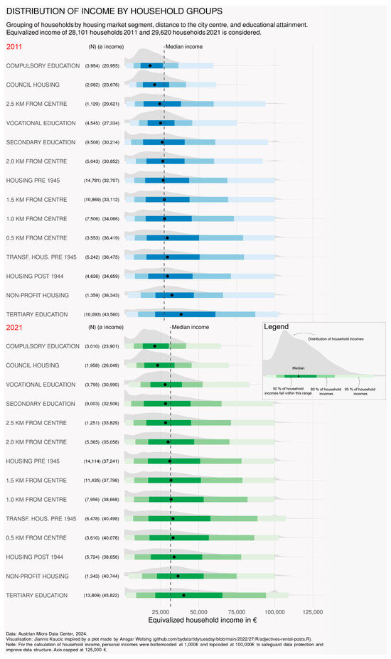
Figure 5.
Distribution of equivalised household income by housing market segment, distance to the city centre, and educational attainment for the years 2011 (top panel) and 2020/21 (bottom panel). Note: For the calculation of household income, personal incomes were bottom-coded at 1000 EUR and top-coded at 100,000 EUR to safeguard data protection and improve data structure. The axis was capped at 125,000 EUR.
For each year, household groups were sorted by their median income in ascending order. In 2011, households displaying compulsory education only, households in council housing, and households in the most peripheral distance band from the city centre had lower median incomes than other households. Furthermore, the generally heavily right-skewed distribution of incomes was less pronounced in these three groups, and the income spread was lower. In contrast, the segments of transformed and non-transformed housing built before 1945, housing built post-1944 and housing provided by limited-profit associations, households living within 2 kilometres from the centre, and households with tertiary education had the highest median incomes and increasingly flat and wide income distributions. The one-way ANOVA test and multiple Tukey pairwise comparisons of group mean values confirmed the visual impression that there were significant differences in income distribution between the group of households living in council housing and all other housing segments (but not between the other segments). In the period 2011–2020/21, differences between the housing market segments remained stable. Furthermore, in both years, differences between housing market segments appeared to be more pronounced than those between central–peripheral distance zones: although there was a decline in average incomes following a distance gradient, the differences in median income and the dispersion of incomes were very small across the five distance zones.
- Regression model
We now turn to the regression analysis at the spatial scale of 100 × 100 m grid cells. The expectation of the multiple regression models is that the income level, its variation, and income segregation in 100 × 100 m grid cells change when the mix of housing market segmentation varies. We ran, separately for 2011 and 2020/21, three regression models with median household income, Gini coefficient, and multi-group local segregation scores as dependent variables and shares of housing market segments as the main explanatory variable of interest. Based on theoretical–conceptual considerations (see the empirical model in Section 3.2), an array of variables representing employment status, educational attainment, migration background, household composition, residential mobility, and location factors were tested as controls. The regression outputs presented in Table 3 represent the best fit models, accounting for multicollinearity issues between explanatory variables (see the correlation matrix in Appendix A for a comprehensive overview of tested variables).
Table 3.
Regression outputs. Notes: ln = natural logarithm; multi-group local segregation scores were multiplied by 1000 to improve legibility of coefficients; 95% confidence intervals in square brackets. We report heteroskedasticity-robust confidence intervals in all models, as the Breusch–Pagan tests indicated heteroscedasticity in the error terms.
Turning to the regression outputs 1 and 2 (Table 3), we observe that in 2011, the share of households in council housing has a significant (p < 0.05) and negative relationship with median income in a grid cell. This was expected, as the below-market rents in this housing segment allow lower-income households to move to these areas. The other housing market segments show non-significant coefficients, rendering their effect not statistically different from zero. The negative relationship between council housing and income loses its significance in 2020/21, which can be partly explained by the diminishing share of council apartments in the area and the in situ upward social mobility of some of the residents with open-ended tenancy agreements. Unexpectedly, in 2020/21, transformed historic housing displays a similarly high and negative correlation with income, which can be explained by the ambiguity of this market segment: residents in this segment could either be renters with a capped rent or owners with presumably higher incomes or other sources of income not registered by wage tax.
Beyond housing variables and for both years of analysis, we observe the expected strong positive relationship between high educational attainment (university degree) and income. Furthermore, a strong negative impact of the share of residential mobility on median incomes in grid cells points to the fact that incoming and outgoing households have a lower income/social status compared to constant residents, which seem to be the drivers of in situ upgrading in some areas [50]. The share of households with different migration backgrounds in the grid cells points to a social succession, with households with backgrounds in the eastern European Union members forming a new migrant group and gaining increasing importance, while ‘traditional’ migrant groups (ex-Yugoslavian and Turkish) decreased in the area. In 2020/21, the share of households with persons born in Eastern European countries and/or holding the citizenship of the respective countries is strongly negatively related to the median income of a grid cell. Lastly, when controlling for housing market segmentation, education, migration background and residential mobility, location factors—here proxied by the mean property price in the neighbourhood—do not have a statistically significant effect on household incomes in the area.
Regression outputs 3 and 4 (Table 3) reveal a negative correlation between the median income level of a grid cell and the Gini coefficient of the same grid cell in both years of analysis. The negative and slightly higher coefficient in 2020/21 points to a homogenisation trend of neighbourhoods with higher median incomes, leading to a lower income gradient within these neighbourhoods. However, the relationship between income and inequality is not strictly linear, but rather follows a more complex pattern. Thus, inequality in a grid cell, as measured by the Gini coefficient, can be driven by the bottom, middle, or top of the income distribution.
The shares of transformed and non-transformed housing built before 1945 show a significant positive correlation with income inequality at the micro scale. This meets our expectations, as these market segments with capped rents create greater social variation within a neighbourhood. In conjunction with evidence on lower income levels within the segment of pre-1945 transformed housing (in 2020/21), we can infer that higher inequality in neighbourhoods with higher shares of this segment mainly relate to the clustering of lower-income groups. This can be explained by the coincidence of owning and renting residents in this segment, confirming existing findings [68]. In 2020/21, the share of households in transformed historic houses had an even stronger positive impact on income inequality compared to 2011. This outcome leads us to assume that, alongside the housing boom during the 2010s and the increasing transformation of the historic housing stock, the historic private housing stock turned out to be a driver of local social mix in terms of variations in the incomes and education of its residents. Council housing produces ambiguous and non-significant results in this study area, and therefore, the effect of this segment on social mix, which was found by other studies [46], cannot be substantiated.
Apart from this result, income inequality in a grid cell is mainly driven by variations in educational attainment and location factors, while it is significantly reduced by higher shares of households with migration backgrounds, especially from ex-Yugoslavian countries, in a neighbourhood. This indicates that groups with similar incomes and migration backgrounds tend cluster in some neighbourhoods, leading to lower social mix. When controlling for the other factors, residential mobility seems to have no impact on income inequality in a neighbourhood. In conjunction with the outcomes in model 1 and 2 of a negative relationship with income levels, which would suggest a positive relationship with inequality, this shows the spatially very selective nature of residential mobility in the area.
Regression outputs 5 and 6 (Table 3) show the drivers of local segregation of income quintile groups. Median household income and income inequality are the main drivers of segregation, with income presenting a U-shaped relationship, as evidenced by the significant second-order polynomial terms. Not only do very high levels of income within grid cells consequently lead to segregation across grid cells, but so do very low levels of income or inequality. It is evident that in order for spatial segregation to exist, there has to be some form of income inequality between individuals or households [28]. This theoretically points towards a positive relationship between the two phenomena. However, the direction of this relationship depends on the configuration of the income distribution that drives inequality within a grid cell compared to the average configuration of income distributions in all other grid cells4. Furthermore, the fact that income variation across households in very small spatial units—as measured by the Gini coefficient—can be much higher and be more strongly influenced by outliers than variation between quintile income groups—as measured by the segregation score—can also influence the relationship between inequality and segregation. Apart from this, for both years, the housing market segments prove to have no additional explanatory value for local income segregation, which is partly due to its correlation with the income variable.
5. Discussion
In this paper, we have analysed the spatial patterns and drivers of income inequality and income segregation at the micro scale. Our main intention was to estimate the influence of housing market segments on the patterns and dynamics of income inequality/segregation. Our analysis at the scale of 100 × 100 m grid cells reveals two main results.
Firstly, household income displays a heterogenous pattern: A general decline alongside the central–peripheral gradient is distorted by clustered areas with a more affluent population, particularly alongside Mariahilfer Straße. Between 2011 and 2020/21, this pattern remained stable or became even more pronounced. Similarly, the spatial pattern also indicates declining income inequality along a central–peripheral gradient. This general pattern is driven by the income gap between central and peripheral neighbourhoods. However, this general picture is distorted by the highly dispersed pattern of grid cells with high or low incomes and income inequality. This points to the fact that we can encounter social inequality even at the micro scale of 100 × 100 m grid cells, which is smaller than the scale of street blocks. Finally, the area of interest displays only weak segregation at the micro scale, which is driven by a very small number of grid cells with a high upward or downward deviation in social status. Altogether, even in this small area, the results confirm high income variation and inequality, which cannot be explained merely by a central–peripheral gradient, contrary to what the classic segregation literature might let us assume [2,3].
Secondly, our analysis reveals a relationship between local housing market segmentation and income distribution in grid cells. Generally, our data indicate a high variation in housing market segments within the area of study, as well as clear social variation between these segments. The contrast between council housing, which represents the lowest median income and income spread, and transformed historic tenement houses, which represent the highest median income and income spread, is obvious. Our regression models indicate that housing market segmentation generally has an impact on income levels, as well as on income inequality, at the micro scale, in particular in 2020/21, at the peak of Vienna’s house-price boom. The share of households in transformed and non-transformed historic tenement houses is significantly related to higher income inequality in the grid cells. However, our models do not reveal any significant impact of housing market segments on income micro-segregation.
Our analysis relies on microdata that link household and building data at the individual scale, which is a methodological novelty, in particular for Vienna. However, microdata on personal income from wage-tax statistics have their limitations in terms of determining the ‘real’ wealth or material well-being of households, which might distort the relationship between housing market segments (and other variables, such as employment status, etc.) and socio-economic inequality and segregation. Also, the ownership status of residents, despite being an important control variable, is omitted from the models due to missing data: In the segments of historic housing built pre-1945 (transformed and non-transformed), as well as housing built post-1944, we do not know if residents are renting with a capped rent, or if they are the owners of the flat. Furthermore, the small study area, which comprises two small inner-city districts, both dominated by two housing market segments (historic tenement houses, transformed and non-transformed) and characterised by a quite homogeneous, wealthy population compared to the city of Vienna as a whole, is a limitation. Thus, the results must be interpreted cautiously. However, despite this limitation, our analysis provides new insights regarding the social structure and dynamic of Vienna’s housing market.
6. Conclusions
The empirical results of this analysis contribute to the debate on residential segregation in two ways. Firstly, we have found that the idea of homogeneous neighbourhoods in the city does not correspond to the socio-economic reality—at least not in Vienna’s inner-city, densely built-up area. Statistical units larger than the street block hide these socio-economic patterns and dynamics at the level of individual buildings. While most studies on micro-segregation focus on the vertical dimension [21,22], this analysis shows that segregation between individual residential buildings likewise has an impact on the social structure and dynamic of a neighbourhood.
Secondly, notwithstanding the dominance of the historic housing stock in the area of interest, we could illustrate that housing market segments have a direct significant influence on income level and inequality at the micro scale and an indirect one on segregation. As segregation is mainly determined by the income distribution in a neighbourhood and the geography of housing market segments within urban space is a significant driver of income levels and inequality, a mediating effect of housing market segments on micro-segregation can be assumed. This confirms existing findings that point to the impact of the social housing segment [36,46], but also highlights the important role of the historic housing stock for social diversity in the neighbourhood.
Both arguments taken together, the main assumptions of urban segregation concepts that rely on the Chicago school must be considered much more critically, in particular for the case of Vienna, but arguably also for many European cities.
These outcomes have conceptual implications, which are relevant for urban planners as well as researchers: In a European city such as Vienna, considering housing market segmentation is crucial for our understanding of the mutual relationship between housing market dynamics and social change. Housing market segments, with their different entry barriers, allocation systems, and ownership structures, not only distort the liberal market mechanism. They also react very differently to general market dynamics, such as a house-price boom or bust. As the transformation of Vienna’s historic housing stock shows in particular, market segments and their patterns in urban space can turn into drivers of income variation and inequality at the neighbourhood level.
Author Contributions
Conceptualization, R.M. and J.K.; methodology, R.M. and J.K.; software, J.K.; validation, R.M.; formal analysis, R.M. and J.K.; investigation, R.M. and J.K.; resources, R.M. and J.K.; data curation, J.K.; writing—original draft preparation, R.M. and J.K.; writing—review and editing, R.M. and J.K.; visualization, J.K.; supervision,; R.M. All authors have read and agreed to the published version of the manuscript.
Funding
This research received no external funding.
Data Availability Statement
Data are contained within the article.
Conflicts of Interest
The authors declare no conflict of interest.
Appendix A. Correlation Matrices
Table A1.
Variables 2011.
Table A1.
Variables 2011.
| 1 | 2 | 3 | 4 | 5 | 6 | 7 | 8 | 9 | 10 | 11 | 12 | 13 | 14 | 15 | 16 | 17 | 18 | 19 | 20 | 21 | 22 | 23 | 24 | 25 | |
|---|---|---|---|---|---|---|---|---|---|---|---|---|---|---|---|---|---|---|---|---|---|---|---|---|---|
| (1) Median income (ln) | 1 | ||||||||||||||||||||||||
| (2) Gini coef-ficient (ln) | −0.13 | 1 | |||||||||||||||||||||||
| (3) Multigroup local segreg. | −0.25 | −0.34 | 1 | ||||||||||||||||||||||
| (4) Share council hous. | −0.32 | −0.24 | 0.28 | 1 | |||||||||||||||||||||
| (5) Share hous. built > 1944 | 0.05 | −0.11 | −0.02 | −0.16 | 1 | ||||||||||||||||||||
| (6) Share hous. built < 1945 | 0.08 | 0.23 | −0.12 | −0.40 | −0.56 | 1 | |||||||||||||||||||
| (7) Share hous. built < 1945, tr. | 0.04 | 0.16 | −0.15 | −0.10 | −0.23 | −0.30 | 1 | ||||||||||||||||||
| (8) Share mig. bg., ex-YU | −0.48 | −0.25 | 0.23 | 0.14 | −0.07 | 0.04 | −0.05 | 1 | |||||||||||||||||
| (9) Share mig. bg., TR | −0.40 | −0.19 | 0.19 | 0.45 | −0.12 | −0.12 | −0.06 | 0.42 | 1 | ||||||||||||||||
| (10) Share mig. bg., EU-East | −0.12 | −0.09 | 0.08 | 0.08 | 0.12 | −0.10 | −0.09 | 0.23 | 0.11 | 1 | |||||||||||||||
| (11) Share mig. bg., World | −0.33 | −0.12 | 0.14 | 0.41 | 0.09 | −0.25 | −0.05 | 0.29 | 0.25 | 0.16 | 1 | ||||||||||||||
| (12) Share univ. degree | 0.61 | 0.31 | −0.33 | −0.44 | −0.01 | 0.20 | 0.18 | −0.60 | −0.44 | −0.22 | −0.37 | 1 | |||||||||||||
| (13) Share res. mob. 2011–21 | −0.31 | 0.11 | 0.06 | −0.20 | 0.16 | 0.10 | −0.03 | 0.20 | −0.03 | 0.05 | 0.07 | −0.04 | 1 | ||||||||||||
| (14) Share full-time employed | 0.30 | −0.20 | −0.10 | −0.21 | 0.24 | −0.13 | 0.04 | 0.01 | −0.05 | 0.07 | −0.08 | 0.14 | 0.05 | 1 | |||||||||||
| (15) Share pensioners | −0.13 | −0.24 | 0.20 | 0.36 | −0.10 | −0.10 | −0.15 | 0.03 | 0.10 | 0.02 | 0.08 | −0.34 | −0.25 | −0.63 | 1 | ||||||||||
| (16) Share marg. empl. | −0.39 | 0.41 | 0.00 | −0.02 | −0.08 | 0.07 | 0.13 | 0.04 | 0.06 | −0.07 | 0.11 | 0.02 | 0.32 | −0.23 | −0.44 | 1 | |||||||||
| (17) Share unemployed | −0.52 | 0.21 | 0.31 | 0.28 | −0.10 | −0.07 | 0.02 | 0.14 | 0.24 | 0.04 | 0.22 | −0.35 | 0.14 | −0.27 | −0.01 | 0.53 | 1 | ||||||||
| (18) Share students | −0.17 | 0.19 | −0.16 | −0.13 | 0.14 | −0.08 | 0.09 | −0.03 | 0.05 | 0.12 | 0.01 | −0.06 | 0.18 | 0.02 | −0.11 | 0.14 | −0.01 | 1 | |||||||
| (19) Average household size | 0.43 | −0.18 | −0.01 | 0.13 | −0.33 | 0.19 | −0.04 | 0.04 | 0.07 | 0.01 | 0.04 | 0.04 | −0.31 | −0.01 | 0.08 | −0.20 | −0.18 | −0.18 | 1 | ||||||
| (20) Income depend. ratio | −0.07 | 0.27 | −0.03 | −0.07 | −0.02 | 0.10 | −0.01 | −0.11 | −0.01 | −0.10 | −0.06 | 0.11 | 0.07 | −0.16 | −0.08 | 0.17 | 0.02 | 0.15 | 0.07 | 1 | |||||
| (21) Popul. dens. (inh./ha) | −0.08 | −0.10 | 0.20 | 0.12 | 0.07 | −0.23 | −0.04 | −0.01 | 0.14 | 0.07 | −0.06 | −0.12 | −0.13 | 0.05 | 0.05 | −0.03 | 0.00 | 0.08 | 0.02 | 0.09 | 1 | ||||
| (22) Mean prop. price (ln) | 0.37 | 0.32 | −0.17 | −0.17 | −0.19 | 0.27 | 0.05 | −0.45 | −0.28 | −0.20 | −0.22 | 0.49 | −0.22 | −0.15 | 0.05 | −0.11 | −0.15 | −0.14 | 0.07 | 0.11 | −0.10 | 1 | |||
| (23) Distance to centre (km) | −0.25 | −0.32 | 0.13 | 0.21 | 0.32 | −0.39 | −0.08 | 0.24 | 0.24 | 0.12 | 0.27 | −0.44 | 0.15 | 0.18 | 0.01 | 0.02 | 0.14 | 0.10 | −0.08 | −0.13 | 0.08 | −0.73 | 1 | ||
| (24) Active mobility score | 0.36 | 0.22 | −0.06 | −0.11 | −0.20 | 0.29 | −0.03 | −0.33 | −0.24 | −0.16 | −0.23 | 0.41 | −0.17 | −0.12 | 0.02 | −0.10 | −0.11 | −0.23 | 0.08 | 0.01 | −0.14 | 0.64 | −0.59 | 1 | |
| (25) Amenity access score | 0.23 | 0.31 | −0.13 | −0.23 | −0.31 | 0.39 | 0.08 | −0.25 | −0.23 | −0.15 | −0.29 | 0.46 | −0.10 | −0.12 | −0.07 | −0.01 | −0.17 | −0.07 | 0.01 | 0.09 | −0.07 | 0.63 | −0.92 | 0.57 | 1 |
Source: Authors; Notes: Pearson correlation coefficient (r); N = 272 100 × 100 m grid cells. Rows/columns 1–3: Dependent variables; rows/columns 4–7: Housing market segments; rows/columns 8–11: Migration background; rows/columns 12: Education; rows/columns 13: Residential mobility; rows/columns 14–18: Employment status; rows/columns 19–21: Household composition; rows/columns 22–25: location factors.
Table A2.
Variables 2020/21.
Table A2.
Variables 2020/21.
| 1 | 2 | 3 | 4 | 5 | 6 | 7 | 8 | 9 | 10 | 11 | 12 | 13 | 14 | 15 | 16 | 17 | 18 | 19 | 20 | 21 | 22 | 23 | 24 | 25 | |
|---|---|---|---|---|---|---|---|---|---|---|---|---|---|---|---|---|---|---|---|---|---|---|---|---|---|
| (1) Median income (ln) | 1 | ||||||||||||||||||||||||
| (2) Gini coef-ficient (ln) | −0.46 | 1 | |||||||||||||||||||||||
| (3) Multigroup local segreg. | −0.15 | −0.27 | 1 | ||||||||||||||||||||||
| (4) Share council hous. | −0.30 | −0.11 | 0.24 | 1 | |||||||||||||||||||||
| (5) Share hous. built > 1944 | 0.08 | −0.16 | −0.01 | −0.15 | 1 | ||||||||||||||||||||
| (6) Share hous. built < 1945 | 0.08 | 0.14 | −0.11 | −0.36 | −0.58 | 1 | |||||||||||||||||||
| (7) Share hous. built < 1945, tr. | 0.00 | 0.26 | −0.15 | −0.16 | −0.28 | −0.27 | 1 | ||||||||||||||||||
| (8) Share mig. bg., ex-YU | −0.46 | −0.04 | 0.20 | 0.26 | −0.02 | −0.06 | −0.11 | 1 | |||||||||||||||||
| (9) Share mig. bg., TR | −0.29 | −0.15 | 0.20 | 0.50 | −0.09 | −0.12 | −0.16 | 0.36 | 1 | ||||||||||||||||
| (10) Share mig. bg., EU-East | −0.31 | 0.09 | 0.10 | 0.07 | 0.19 | −0.12 | −0.11 | 0.24 | 0.20 | 1 | |||||||||||||||
| (11) Share mig. bg., World | −0.32 | 0.02 | 0.13 | 0.43 | 0.13 | −0.25 | −0.08 | 0.28 | 0.36 | 0.20 | 1 | ||||||||||||||
| (12) Share univ. degree | 0.60 | 0.07 | −0.28 | −0.54 | 0.07 | 0.16 | 0.22 | −0.57 | −0.43 | −0.26 | −0.41 | 1 | |||||||||||||
| (13) Share res. mob. 2011–21 | −0.17 | 0.19 | 0.11 | −0.16 | 0.38 | −0.12 | −0.07 | 0.08 | −0.06 | 0.17 | 0.13 | 0.15 | 1 | ||||||||||||
| (14) Share full-time employed | 0.22 | −0.18 | −0.08 | −0.23 | 0.39 | −0.20 | −0.03 | −0.03 | −0.12 | 0.04 | −0.01 | 0.24 | 0.45 | 1 | |||||||||||
| (15) Share pensioners | −0.05 | −0.17 | 0.10 | 0.22 | −0.13 | −0.03 | −0.09 | 0.05 | 0.12 | −0.06 | 0.02 | −0.37 | −0.62 | −0.59 | 1 | ||||||||||
| (16) Share marg. empl. | −0.31 | 0.36 | 0.05 | 0.07 | −0.13 | 0.11 | 0.03 | 0.08 | 0.08 | 0.08 | 0.05 | −0.07 | 0.30 | −0.16 | −0.46 | 1 | |||||||||
| (17) Share unemployed | −0.51 | 0.15 | 0.29 | 0.50 | −0.14 | −0.06 | −0.12 | 0.32 | 0.40 | 0.28 | 0.27 | −0.44 | 0.06 | −0.21 | −0.01 | 0.34 | 1 | ||||||||
| (18) Share students | −0.20 | 0.24 | −0.11 | −0.01 | −0.05 | 0.08 | 0.01 | 0.03 | −0.05 | −0.03 | −0.04 | −0.04 | 0.13 | −0.07 | −0.09 | 0.41 | −0.04 | 1 | |||||||
| (19) Average household size | 0.42 | −0.23 | 0.03 | 0.14 | −0.31 | 0.22 | −0.05 | 0.06 | 0.19 | −0.14 | −0.07 | 0.02 | −0.25 | −0.14 | 0.15 | −0.08 | −0.03 | −0.09 | 1 | ||||||
| (20) Income depend. ratio | −0.09 | 0.34 | 0.03 | −0.10 | −0.04 | 0.14 | 0.02 | −0.16 | −0.10 | 0.00 | −0.04 | 0.02 | 0.14 | −0.12 | −0.05 | 0.18 | 0.01 | 0.09 | −0.06 | 1 | |||||
| (21) Popul. dens. (inh./ha) | −0.08 | −0.12 | 0.18 | 0.10 | 0.13 | −0.29 | 0.02 | 0.03 | 0.08 | 0.09 | 0.02 | −0.12 | 0.01 | 0.08 | −0.02 | −0.01 | 0.04 | −0.03 | 0.01 | −0.12 | 1 | ||||
| (22) Mean prop. price (ln) | 0.40 | 0.10 | −0.13 | −0.27 | −0.21 | 0.34 | 0.06 | −0.50 | −0.29 | −0.28 | −0.31 | 0.49 | −0.19 | −0.15 | 0.04 | −0.09 | −0.25 | −0.11 | 0.13 | 0.17 | −0.15 | 1 | |||
| (23) Distance to centre (km) | −0.27 | −0.12 | 0.09 | 0.25 | 0.30 | −0.40 | −0.09 | 0.34 | 0.22 | 0.26 | 0.31 | −0.43 | 0.16 | 0.19 | 0.01 | 0.00 | 0.21 | 0.04 | −0.11 | −0.17 | 0.13 | −0.85 | 1 | ||
| (24) Active mobility score | 0.38 | −0.01 | −0.02 | −0.15 | −0.16 | 0.31 | −0.07 | −0.32 | −0.22 | −0.28 | −0.22 | 0.36 | −0.14 | −0.15 | 0.09 | −0.10 | −0.22 | −0.16 | 0.11 | 0.10 | −0.20 | 0.67 | −0.59 | 1 | |
| (25) Amenity access score | 0.28 | 0.12 | −0.08 | −0.27 | −0.27 | 0.39 | 0.09 | −0.33 | −0.26 | −0.32 | −0.32 | 0.43 | −0.13 | −0.15 | −0.03 | −0.01 | −0.26 | −0.02 | 0.06 | 0.16 | −0.12 | 0.81 | −0.92 | 0.58 | 1 |
Source: Authors; Notes: Pearson correlation coefficient (r); N = 272 100 × 100 m grid cells. Rows/columns 1–3: Dependent variables; rows/columns 4–7: Housing market segments; rows/columns 8–11: Migration background; rows/columns 12: Education; rows/columns 13: Residential mobility; rows/columns 14–18: Employment status; rows/columns 19–21: Household composition; rows/columns 22–25: location factors.
Notes
| 1 | Table 1 shows all variables included in the final regression analyses. Many more variables were tested as controls based on theoretical–conceptual considerations (see Section 3.2), but they were excluded from the final models due to issues of multicollinearity and overfitting; see the correlation matrix in the Appendix A for a comprehensive overview of tested variables. |
| 2 | As opposed to Theil’s information theory index H, the Mutual Information Index M is not normalised between 0 and 1, but it is the preferred segregation index to decompose global segregation into local segregation scores, indicating the contribution to overall segregation. |
| 3 | In this case, we use Theil’s H index instead of the Mutual Information Index M, because it has methodological advantages for analysing composite (aggregate) segregation [60]. |
| 4 | For the decomposition of segregation into local segregation scores, the distribution of households across income quintiles was analysed in each grid cell and compared to all other cells. Therefore, grid cells with the over- OR under-representation of certain income quintiles compared to the global average receive higher local segregation scores. |
References
- Musterd, S. Urban Segregation: Contexts, Domains, Dimensions and Approaches. In Handbook of Urban Segregation; Musterd, S., Ed.; Edward Elgar Publishing: Cheltenham, UK; Northampton, MA, USA, 2020; pp. 2–17. [Google Scholar]
- Lichtenberger, E. Stadtgeographie 1. Begriffe, Konzepte, Modelle, Prozesse; Teubner Studienbücher, Geographie; Teubner: Stuttgart, Germany, 1991. [Google Scholar]
- Maloutas, T. The Role of Vertical Segregation in Urban Social Processes. Nat. Cities 2024, 1, 185–193. [Google Scholar] [CrossRef]
- Benevolo, L. Die Stadt in der Europäischen Geschichte; Beck: München, Germany, 1993. [Google Scholar]
- Lichtenberger, E. Wem Gehört Die Dritte Dimension in Der Stadt. Mitteilungen Österr. Geogr. Ges. 2001, 143, 7–34. [Google Scholar]
- Logan, J.R.; Bellman, B. Before The Philadelphia Negro: Residential Segregation in a Nineteenth-Century Northern City. Soc. Sci. Hist. 2016, 40, 683–706. [Google Scholar] [CrossRef] [PubMed]
- Logan, J.R.; Martinez, M. The Spatial Scale and Spatial Configuration of Residential Settlement: Measuring Segregation in the Postbellum South. AJS 2018, 123, 1161–1203. [Google Scholar] [CrossRef] [PubMed]
- Maloutas, T.; Karadimitriou, N. Introduction to Vertical Cities: Urban Micro-Segregation, Housing Markets and Social Reproduction. In Vertical Cities; Edward Elgar Publishing: Cheltenham, UK; Northampton, MA, USA, 2022; pp. 1–21. [Google Scholar]
- Ghertner, D.A. Why Gentrification Theory Fails in ‘Much of the World’. City 2015, 19, 552–563. [Google Scholar] [CrossRef]
- Kemeny, J.; Kersloot, J.; Thalmann, P. Limited-profit Housing Influencing, Leading and Dominating the Unitary Rental Market: Three Case Studies. Hous. Stud. 2005, 20, 855–872. [Google Scholar] [CrossRef]
- Skifter Andersen, H.; Andersson, R.; Wessel, T.; Vilkama, K. The Impact of Housing Policies and Housing Markets on Ethnic Spatial Segregation: Comparing the Capital Cities of Four Nordic Welfare States. Int. J. Hous. Policy 2016, 16, 1–30. [Google Scholar] [CrossRef]
- Arbaci, S. Ethnic Segregation, Housing Systems and Welfare Regimes in Europe. Eur. J. Hous. Policy 2007, 7, 401–433. [Google Scholar] [CrossRef]
- Statistik Austria: Austrian Micro Data Center (AMDC). Available online: https://www.statistik.at/en/services/tools/services/center-for-science/austrian-micro-data-center-amdc (accessed on 24 June 2024).
- Plank, L.; Schneider, A.; Kadi, J. Wohnbauboom in Wien 2018–2021. Preise, Käufer:Innen Und Leerstände in Der Wohnbauproduktion; Stadtpunkte; Kammer für Arbeiter und Angestellte für Wien: Wien, Austria, 2022. [Google Scholar]
- Harvey, J.; Jowsey, E. Urban Land Economics, 6th ed.; Palgrave Macmillan: Basingstoke, UK, 2004. [Google Scholar]
- Matznetter, W.; Musil, R.; Hitz, H. Hoch Hinaus. Donau City Wien—Hochhausbau Und Stadtentwicklung; Medienbegleitheft zur DVD des BMBF Medienservice Nr. 1415; BMBF: Wien, Austria, 2015. [Google Scholar]
- Unterdorfer, D. “I have no contact to other inhabitants …” Social mixing in a Viennese district—The dichotomy of a concept. Mitteilungen Österr. Geogr. Ges. 2016, 158, 109–132. [Google Scholar] [CrossRef]
- Marcińczak, S.; Hess, D.B. Vertical Separation in High-Rise Apartment Buildings: Evidence from Bucharest and Budapest under State Socialism. In Vertical Cities; Edward Elgar Publishing: Cheltenham, UK; Northampton, MA, USA, 2022; pp. 173–188. [Google Scholar]
- López-Morales, E.; Abarca, I.A. Perceived Pull and Push Forces in High-Rise Developing Neighborhoods in Santiago, Chile. In Vertical Cities; Edward Elgar Publishing: Cheltenham, UK; Northampton, MA, USA, 2022; pp. 313–317. [Google Scholar]
- Forrest, R.; Tong, K.S.; Wang, W. Residential Stratification and Segmentation in the Hyper-Vertical City. In Handbook of Urban Segregation; Musterd, S., Ed.; Edward Elgar Publishing: Cheltenham, UK; Northampton, MA, USA, 2020; pp. 346–365. [Google Scholar]
- Maloutas, T.; Spyrellis, S.; Karadimitriou, N. Measuring and Mapping Vertical Segregation in Athens. In Vertical Cities; Edward Elgar Publishing: Cheltenham, UK; Northampton, MA, USA, 2022; pp. 88–97. [Google Scholar]
- Myofa, N. Micro-Segregation and Residential Mobility: Case Study of Two Athenian Apartment Blocks. J. Hous. Built Environ. 2023, 38, 2773–2791. [Google Scholar] [CrossRef]
- Meyer, A.; Pfirsch, T. Flat by Flat: Producing Micro-Scale Social Differentiation in an Arrival Neighbourhood of Marseille. In Vertical Cities; Edward Elgar Publishing: Cheltenham, UK; Northampton, MA, USA, 2022; pp. 39–56. [Google Scholar]
- Dines, N.; Mattiucci, C. Constantly Evoked but Under-Researched: The Conundrum of Vertical Stratification in Naples. In Vertical Cities; Edward Elgar Publishing: Cheltenham, UK; Northampton, MA, USA, 2022; pp. 23–38. [Google Scholar]
- Pfirsch, T. Controlling the Proximity of the Poor: Patterns of Micro-Segregation in Naples’ Upper-Class Areas. Land 2023, 12, 2005. [Google Scholar] [CrossRef]
- Wade, R.C. Slavery in the Cities: The South, 1820–1860; Oxford University Press: New York, NY, USA, 1964. [Google Scholar]
- Glaeser, E.L.; Gyourko, J. Arbitrage in Housing Markets; National Bureau of Economic Research: Cambridge, MA, USA, 2007. [Google Scholar]
- Reardon, S.F.; Bischoff, K. Income Inequality and Income Segregation. Am. J. Sociol. 2011, 116, 1092–1153. [Google Scholar] [CrossRef] [PubMed]
- D’Acci, L. Quality of Urban Area, Distance from City Centre, and Housing Value. Case Study on Real Estate Values in Turin. Cities 2019, 91, 71–92. [Google Scholar] [CrossRef]
- Wu, W.; Dong, G.; Zhang, W. The Puzzling Heterogeneity of Amenity Capitalization Effects on Land Markets. Pap. Reg. Sci. 2017, 96, 135–154. [Google Scholar] [CrossRef]
- Herath, S.; Choumert, J.; Maier, G. The Value of the Greenbelt in Vienna: A Spatial Hedonic Analysis. Ann. Reg. Sci. 2015, 54, 349–374. [Google Scholar] [CrossRef]
- Morawetz, U.B.; Klaiber, H.A. Does Housing Policy Impact Income Sorting near Urban Amenities? Evidence from Vienna, Austria. Ann. Reg. Sci. 2022, 69, 411–454. [Google Scholar] [CrossRef]
- Allen, J.; Barlow, J.; Leal, J.; Maloutas, T.; Padovani, L. Introduction. In Housing and Welfare in Southern Europe; Allen, J., Barlow, J., Leal, J., Maloutas, T., Padovani, L., Eds.; John Wiley & Sons, Ltd.: Hoboken, NJ, USA, 2004; pp. 1–13. [Google Scholar]
- Kemeny, J. Corporatism and Housing Regimes. Hous. Theory Soc. 2006, 23, 1–18. [Google Scholar] [CrossRef]
- Rothenberg, J.; Galster, G.C.; Butler, R.V.; Pitkin, J.R. The Maze of Urban Housing Markets: Theory, Evidence, and Policy; University of Chicago Press: Chicago, IL, USA, 1991. [Google Scholar]
- Aufhauser, E.; Giffinger, R.; Knoetig, G. Effects of the Housing Rehabilitation Act on Housing Market Segmentation in Vienna. In Spatial Analysis and Population Dynamics; Pumain, D., Ed.; John Libbey: London, UK; Rome, Italy, 1991; pp. 357–372. [Google Scholar]
- Musterd, S.; Andersson, R. Housing Mix, Social Mix, and Social Opportunities. Urban Aff. Rev. 2005, 40, 761–790. [Google Scholar] [CrossRef]
- Murie, A.; Musterd, S. Social Segregation, Housing Tenure and Social Change in Dutch Cities in the Late 1980s. Urban Stud. 1996, 33, 495–516. [Google Scholar] [CrossRef]
- Kesteloot, C.; Cortie, C. Housing Turks and Moroccans in Brussels and Amsterdam: The Difference between Private and Public Markets. Urban Stud. 1998, 35, 1835–1853. [Google Scholar] [CrossRef]
- Matznetter, W. 100 Jahre Mieterschutz: Ein Instrument Zur Steuerung von Gentrifizierung. In Gentrifizierung in Wien. Perspektiven aus Wissenschaft, Politik und Praxis? Kadi, J., Verlič, M., Eds.; Standpunkte 27; Arbeiterkammer Wien: Wien, Austria, 2019; pp. 13–24. [Google Scholar]
- Kohlbacher, J.; Reeger, U. Die Dynamik Ethnischer Wohnviertel in Wien. Eine Sozialräumliche Longitudinalanalyse 1981 Und 2005; ISR Forschungsbericht 33; Verlag der Österreichischen Akademie der Wissenschaften: Wien, Austria, 2006. [Google Scholar]
- Musil, R.; Brand, F.; Huemer, H.; Köck, P.; Wonaschütz, M. Die Transformation Der Wiener Gründerzeitstadt. Dynamiken Am Wiener Zinshausmarkt 2007–2019; ISR Forschungsbericht 55; Verlag der Österreichischen Akademie der Wissenschaften: Wien, Austria, 2021. [Google Scholar]
- Clark, E. On Gaps in Gentrification Theory. Hous. Stud. 1992, 7, 16–26. [Google Scholar] [CrossRef]
- Giffinger, R. Segregation in Vienna: Impacts of Market Barriers and Rent Regulations. Urban Stud. 1998, 35, 1791–1812. [Google Scholar] [CrossRef]
- Hatz, G.; Kohlbacher, J.; Reeger, U. Socio-Economic Segregation in Vienna: A Social-Oriented Approach to Urban Planning and Housing. In Socio-Economic Segregation in European Capital Cities: East Meets West; Tammaru, T., Marcinczak, S., Van Ham, M., Eds.; Routledge: London, UK; New York, NY, USA, 2015; pp. 80–109. [Google Scholar]
- Premrov, T.; Schnetzer, M. Social Mix and the City: Council Housing and Neighbourhood Income Inequality in Vienna. Urban Stud. 2023, 60, 752–769. [Google Scholar] [CrossRef]
- Kadi, J.; Banabak, S.; Schneider, A. Widening Gaps? Socio-Spatial Inequality in the “Very” European City of Vienna since the Financial Crisis. Cities 2022, 131, 103887. [Google Scholar] [CrossRef]
- Gray, D. Convergence and Divergence in British Housing Space. Reg. Stud. 2018, 52, 901–910. [Google Scholar] [CrossRef]
- Tammaru, T.; Musterd, S.; van Ham, M.; Marcińczak, S. A Multifactor Approach to Understanding Socio-Economic Segregation in European Capital Cities. In Socio-Economic Segregation in European Capital Cities: East Meets West; Tammaru, T., Marcińczak, S., van Ham, M., Musterd, S., Eds.; Routledge: London, UK, 2015; pp. 1–29. [Google Scholar]
- Bailey, N. How Spatial Segregation Changes over Time: Sorting Out the Sorting Processes. Environ. Plan. Econ. Space 2012, 44, 705–722. [Google Scholar] [CrossRef]
- Hlasny, V.; Ceriani, L.; Verme, P. Bottom Incomes and the Measurement of Poverty and Inequality. Rev. Income Wealth 2022, 68, 970–1006. [Google Scholar] [CrossRef]
- Van Kerm, P. Extreme Incomes and the Estimation of Poverty and Inequality Indicators from EU-SILC; IRISS Working Paper Series 2007-01; CEPS/INSTEAD: Luxembourg, 2007. [Google Scholar]
- Piketty, T.; Saez, E. Income Inequality in the United States, 1913–1998. Q. J. Econ. 2003, 118, 1–41. [Google Scholar] [CrossRef]
- Couture, V.; Gaubert, C.; Handbury, J.; Hurst, E. Income Growth and the Distributional Effects of Urban Spatial Sorting. Rev. Econ. Stud. 2024, 91, 858–898. [Google Scholar] [CrossRef]
- OECD. OECD Income (IDD) and Wealth (WDD) Distribution Databases; OECD: Paris, France, 2024. [Google Scholar]
- Dixon, P.M.; Weiner, J.; Mitchell-Olds, T.; Woodley, R. Bootstrapping the Gini Coefficient of Inequality. Ecology 1987, 68, 1548–1551. [Google Scholar] [CrossRef]
- Mora, R.; Ruiz-Castillo, J. Entropy-Based Segregation Indices. Sociol. Methodol. 2011, 41, 159–194. [Google Scholar] [CrossRef]
- R Core Team. R: A Language and Environment for Statistical Computing; R Foundation for Statistical Computing: Vienna, Austria, 2021. [Google Scholar]
- Signorell, A. DescTools: Tools for Descriptive Statistics; R Package Version 0.99.54; 2024. Available online: https://github.com/AndriSignorell/DescTools/ (accessed on 24 June 2024).
- Elbers, B. A Method for Studying Differences in Segregation Across Time and Space. Sociol. Methods Res. 2023, 52, 5–42. [Google Scholar] [CrossRef]
- Ahlfeldt, G.M.; Pietrostefani, E. The Economic Effects of Density: A Synthesis. J. Urban Econ. 2019, 111, 93–107. [Google Scholar] [CrossRef]
- Tamaru, T.; Marcinczak, S.; Aunap, R.; vanHam, M.; Janssen, H. Relationship between income inequality and residential segregation of socioeconomic groups. Reg. Stud. 2020, 54, 450–461. [Google Scholar] [CrossRef]
- Schnelzer, J. Praktiken der versteckten Gentrifizierung—Eine Erhebung raumbezogener Adaptionspraktiken von Langzeitbewohnern im gentrifizierten Wiener Stadtraum mittels reflexiver Fotografie. Mitteilungen Österr. Geogr. Ges. 2022, 163, 141–170. [Google Scholar] [CrossRef]
- City of Vienna. Statistisches Jahrbuch Der Stadt Wien 2022; City of Vienna: Wien, Austria, 2022. [Google Scholar]
- Theil, H.; Finizza, A.J. A Note on the Measurement of Racial Integration of Schools by Means of Informational Concepts. J. Math. Sociol. 1971, 1, 187–193. [Google Scholar] [CrossRef]
- Beaubrun-Diant, K.; Maury, T.-P. Income Segregation in France: A Geographical Decomposition across and within Urban Areas. Reg. Stud. 2024, 58, 442–454. [Google Scholar] [CrossRef]
- OECD. Divided Cities: Understanding Intra-Urban Inequalities; Organisation for Economic Co-operation and Development: Paris, France, 2018. [Google Scholar]
- Musil, R.; Brand, F.; Huemer, H.; Wonaschütz, M. The Zinshaus Market and Gentrification Dynamics: The Transformation of the Historic Housing Stock in Vienna, 2007–2019. Urban Stud. 2022, 59, 974–994. [Google Scholar] [CrossRef]
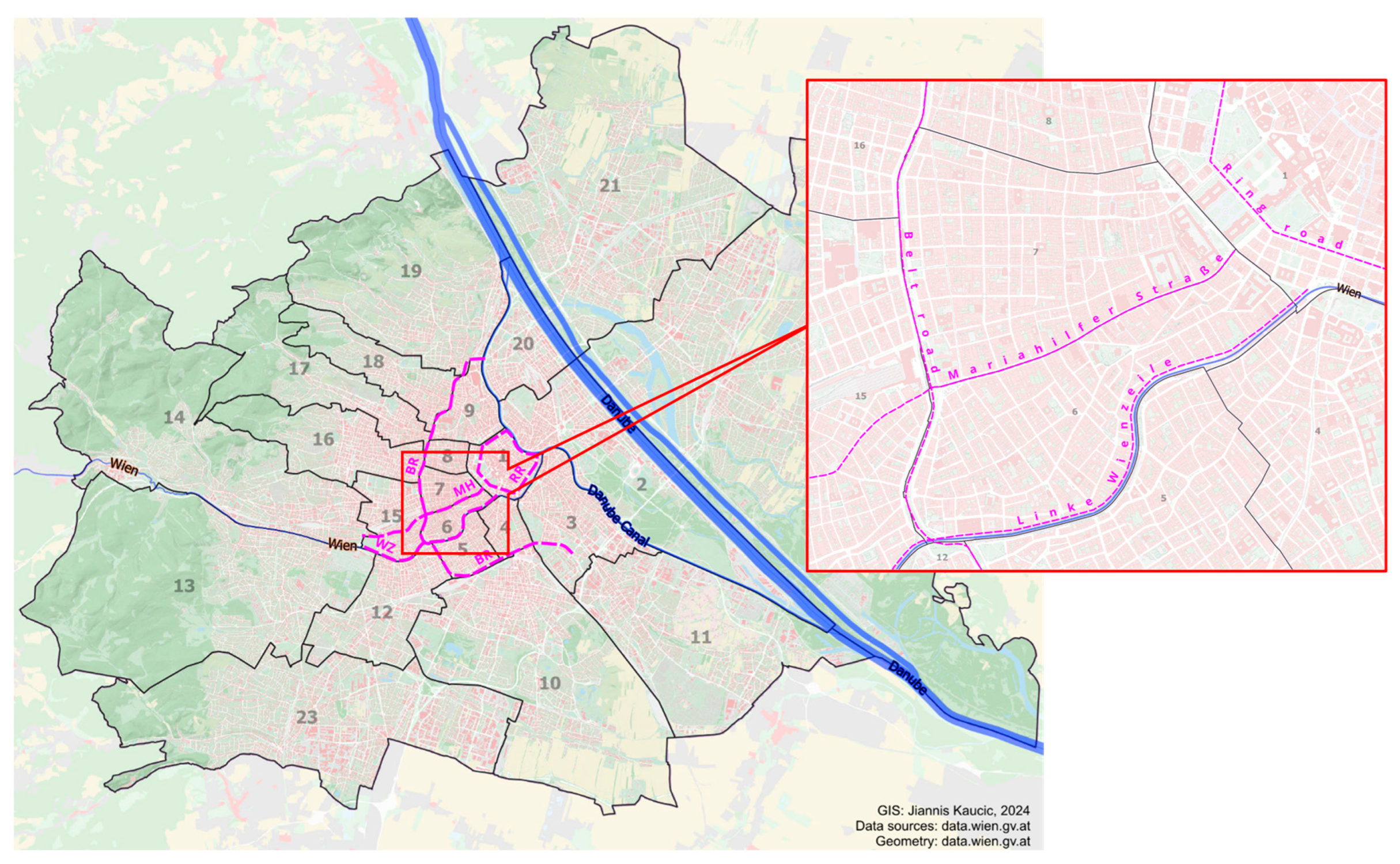
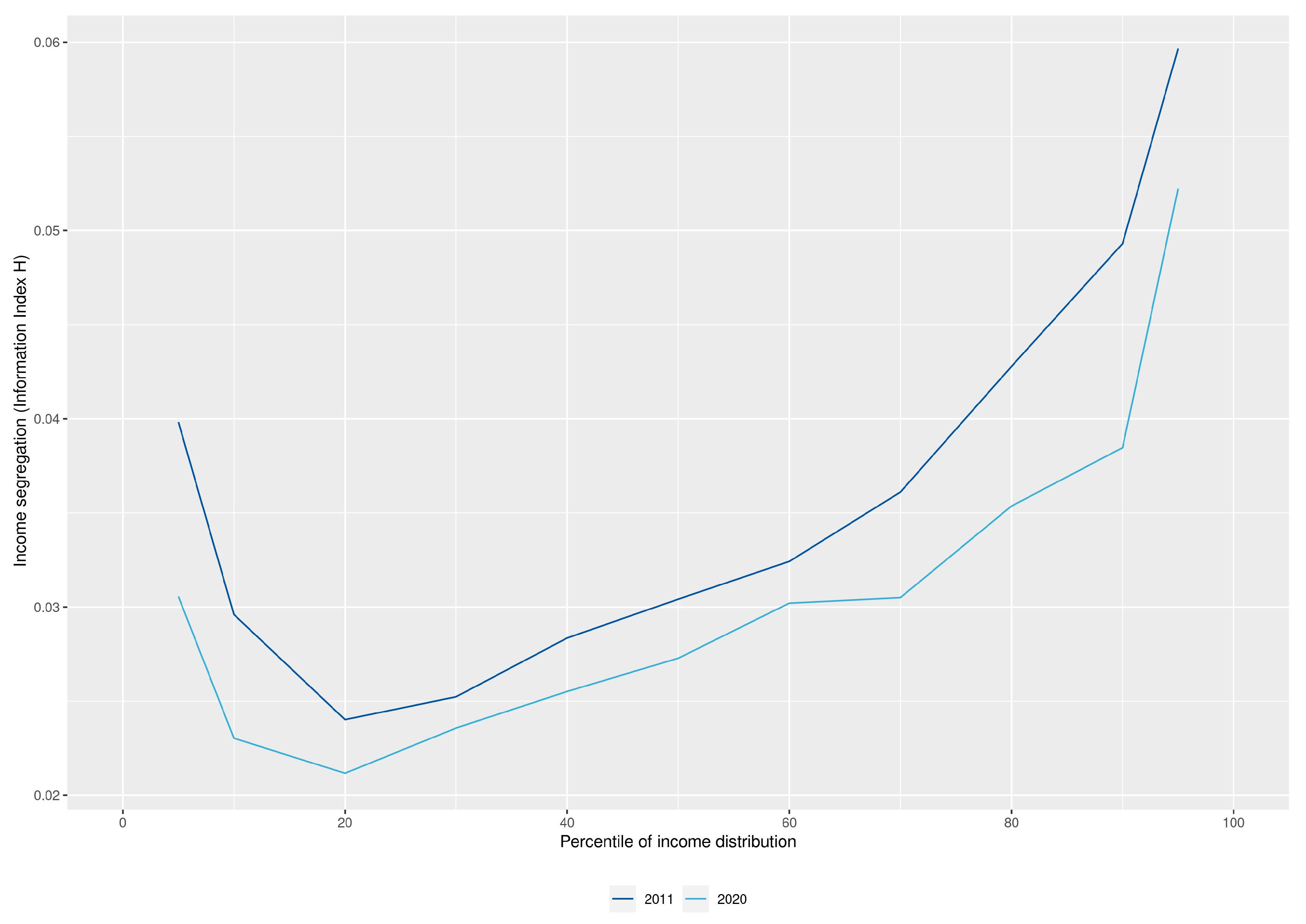
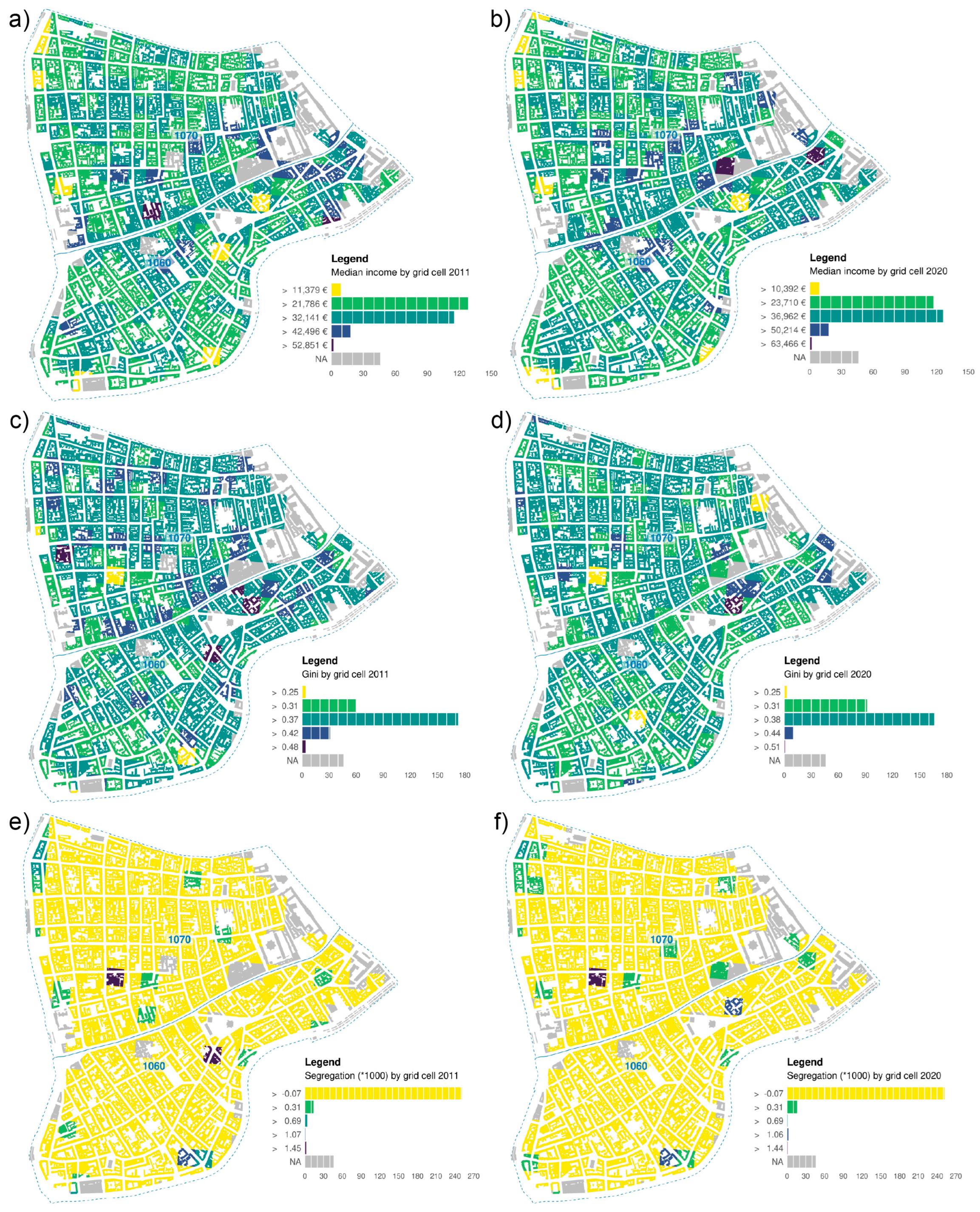
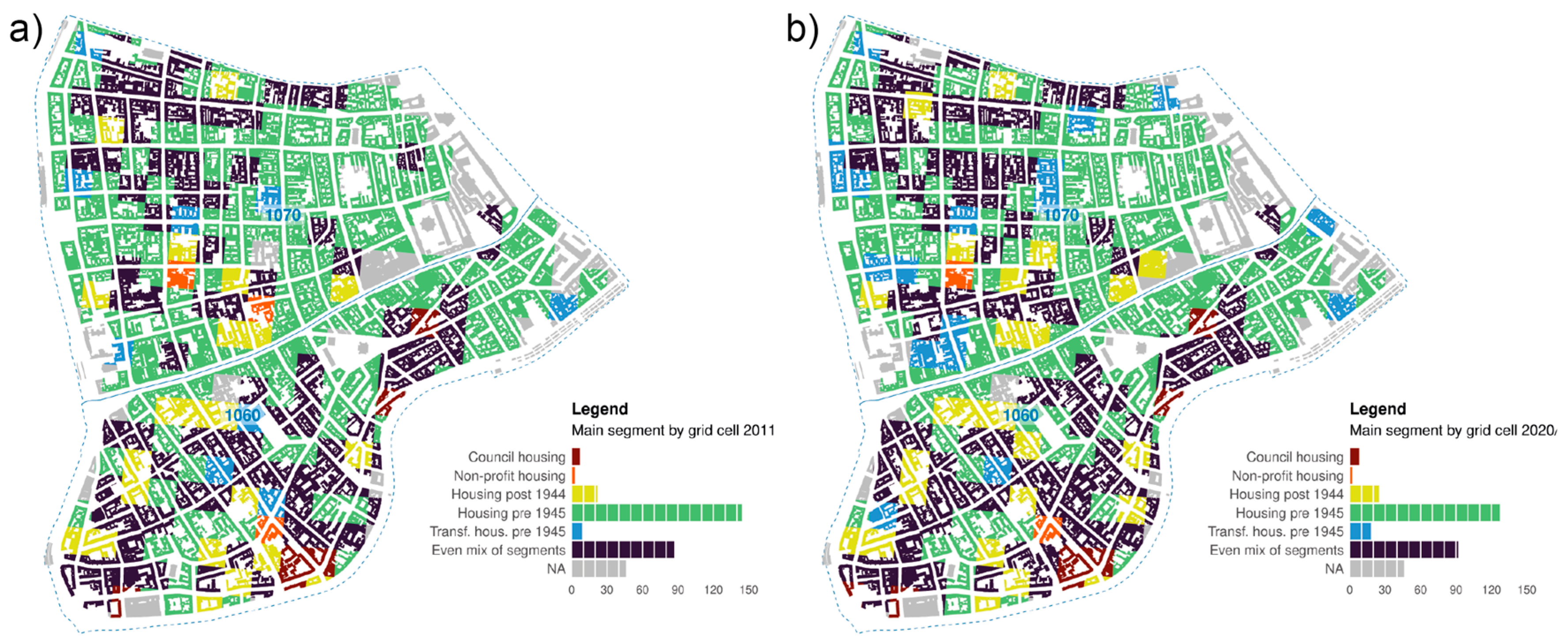
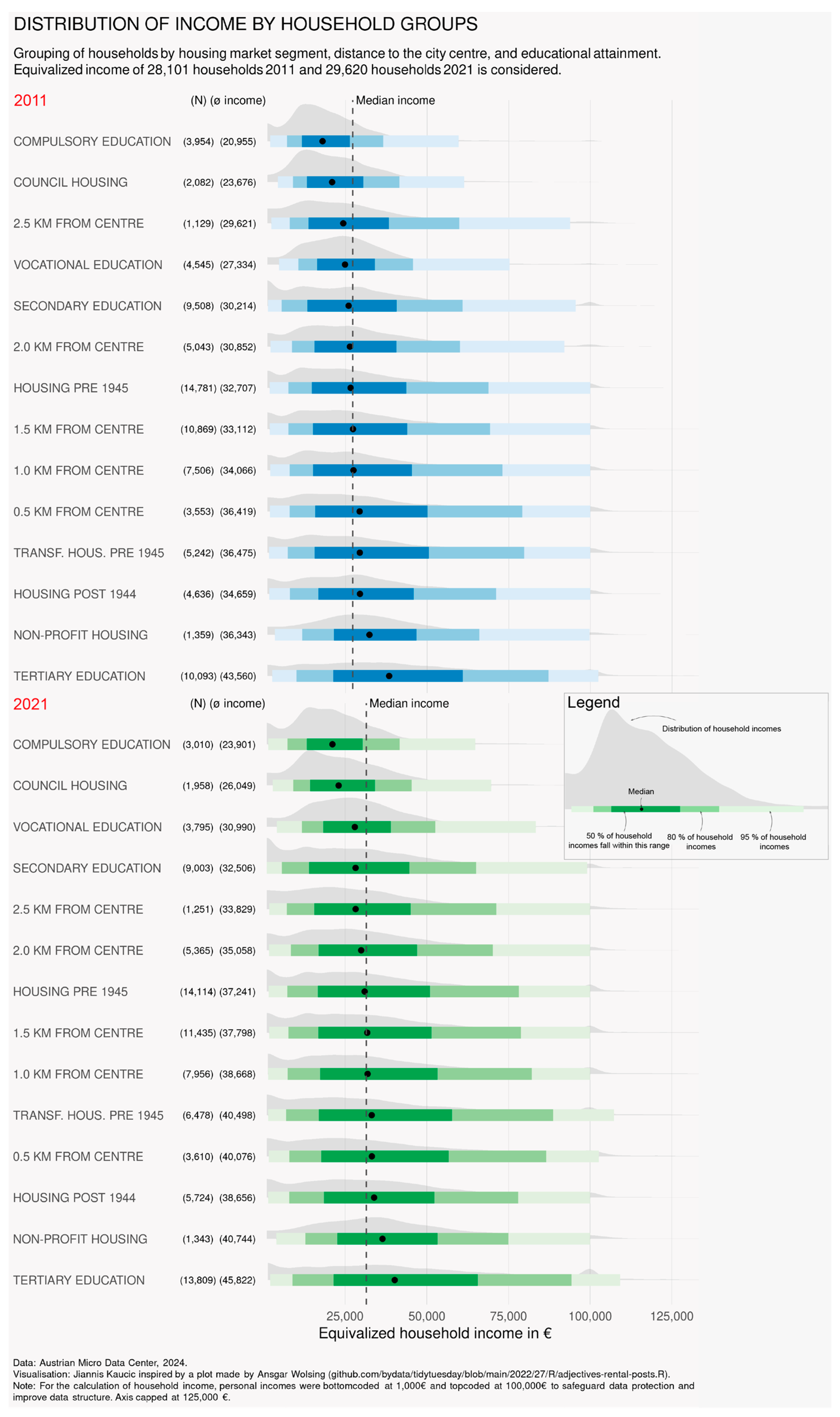
Disclaimer/Publisher’s Note: The statements, opinions and data contained in all publications are solely those of the individual author(s) and contributor(s) and not of MDPI and/or the editor(s). MDPI and/or the editor(s) disclaim responsibility for any injury to people or property resulting from any ideas, methods, instructions or products referred to in the content. |
© 2024 by the authors. Licensee MDPI, Basel, Switzerland. This article is an open access article distributed under the terms and conditions of the Creative Commons Attribution (CC BY) license (https://creativecommons.org/licenses/by/4.0/).