Driving the Evolution of Land Use Patterns: The Impact of Urban Agglomeration Construction Land in the Yangtze River Delta, China

Abstract

The rapid increase in population and economic activities has greatly influenced land use and spatial development. In urban agglomerations where socioeconomic activities are densely concentrated, the clash between ecological protection and economic growth is becoming more evident. Therefore, a thorough quantitative assessment of spatial changes driven by land use dynamics, alongside an examination of temporal and spatial driving factors, is crucial in offering scientific backing for the long-term and sustainable growth of urban agglomerations. This paper focuses on the major urban agglomerations in China’s Yangtze River Delta region, examining the spatiotemporal evolution of land use and landscape patterns from 2000 to 2020. By employing the standard deviation ellipse technique, coupled with multiple linear regression and the geographical detector model, we conduct a quantitative assessment of the directional trends in urban construction land expansion as well as the diverse impacts of temporal and spatial factors on this expansion across various periods and regions. The findings indicate that over the past 20 years, construction land in the Yangtze River Delta Urban Agglomeration expanded in concentrated patches, showing significant scale effects with relatively intact farmland and forest land being increasingly encroached upon. Landscape-type transitions predominantly occurred in cities around Taihu Lake and Hangzhou Bay, with the most significant transition being farmland converted to construction land, resulting in a greater number of patches and more pronounced land fragmentation. Throughout the 20 years, the standard deviation ellipse of construction land in the Yangtze River Delta Urban Agglomeration expanded and shifted, with the predominant expansion trending from the northwest toward the southeast, and the EN orientation being the most intense expansion area, covering 1641.24 km². The influence of temporal and spatial driving factors on the expansion of urban construction land differed across various periods and regions. This study thoroughly examines the driving factors that affect the evolution of urban construction land in the region, offering valuable scientific evidence and references for future planning and development of the Yangtze River Delta Urban Agglomeration, aiding in the formulation of more precise and efficient urban management and land use strategies.

1. Introduction

Land use and spatial evolution have always been the focus of urban research [1,2]. According to United Nations projections, by 2050, almost 70% of the world’s population is expected to live in urban areas [3,4]. Economic growth has driven urban expansion and the redistribution of land resources. In economically advanced regions such as Europe, North America, and parts of Asia, urbanization has converted traditional agricultural land into residential, commercial, and industrial uses. This shift encompasses alterations in land cover as well as modifications in land ownership, usage intensity, and management policies. Consequently, with the development of global cities, identifying land changes and their prudent use have emerged as critical concerns in spatial planning [5,6].

Currently, the harmonious coexistence of land development and ecological environment has become a significant focus in disciplines such as urban planning, geography, and landscape ecology within the background of spatial planning. Optimizing the spatial development and conservation patterns is a key strategic objective in advancing ecological civilization [7,8]. Large ecological patches and corridors in urban and rural ecological spaces are key for species migration and are areas of high ecological risk, but they are also the most vulnerable to encroachment during rapid urban development [9,10]. Agricultural spaces, especially those near towns and roads, are often encroached upon, and the “land compensation balance” policy often suffers from severe “taking the best and giving the worst” issues in its implementation [11]. In China, the primary goal of agricultural space protection, the control and protection of arable land, faces new challenges in the new era, such as the separation of land use and quality construction, singularity of protection measures, and contradictions in territorial space control [12]. As the interaction between human activities and natural ecosystems becomes more intricate, the differentiation in the coupled dynamics of human and natural systems intensifies over time. Additionally, the temporal variations in the coupling process become more evident with increasing complexity in the human–land system [13]. Hence, recognizing the significance of the interplay between natural resources and the macroeconomy, aligning human activities with natural, ecological, climatic, and hydrological factors, and overseeing these interactions across spatial and temporal dimensions are essential for sustaining a cohesive regional framework in territorial planning [14,15].

China’s swift urbanization and industrialization, as the world’s most populous developing nation, have drawn significant international focus. As urbanization continues in China, the Yangtze River Delta Urban Agglomeration (hereinafter referred to as “YRDUR”), a prime example of regions with dense populations and intense socioeconomic activities in the eastern coastal areas, encounters substantial conflicts between the needs for ecological conservation and economic growth. Issues such as conflicts among ecological, urban, and agricultural spaces threaten the region’s sustainable development [16,17,18]. With the increasing trend of regional integration, the interconnections between urban spaces have intensified, exacerbating the “fragmentation” risks facing ecological and agricultural spaces in the Yangtze River Delta (hereinafter referred to as “YRD”). This necessitates enhanced demands for the integrity, systematicness, differentiation, and dynamism of regional spatial planning and control [19,20]. With the ongoing regional integration in China, the growth of urban areas has entered a stock phase, necessitating an urgent transformation and deepening of the logic and methods of spatial control.

Current research on key urban agglomerations in the YRD emphasize carbon emissions [21,22,23], land use efficiency [24,25,26], and landscape patterns (hereinafter referred to as “LSP”) [27,28,29]. For example, Luo Haizhi developed a novel model for characterizing and predicting carbon emissions, which combines explainable machine learning techniques with land use data to project emissions in the YRD [22]. Yang Changyong investigated the mechanisms promoting the synergistic development between population and land by implementing effective green urban land management practices in the area [25]. Zhou Zhechen examined LSP changes in the YRD from 2000 to 2020 using landscape dynamics and pattern indices [29]. Nonetheless, within the background of ecological civilization, there is a research gap regarding the evolution patterns of territorial space and their driving factors in the region, where intensive land use has triggered various environmental and social issues [29,30]. Hence, our research intends to use the core urban agglomerations in the YRD as empirical subjects to accomplish two primary goals: firstly, to utilize remote sensing data to investigate the land use changes and LSPs from 2000 to 2020, elucidating land evolution trends in the developed region; secondly, to explore the patterns of urban construction land (hereinafter referred to as “CTL”) expansion and the driving factors behind its spatiotemporal evolution in major urban agglomerations.

By employing the standard deviation ellipse (hereinafter referred to as “SDE”) method, multiple linear regression (hereinafter referred to as “MLR”), and the geographical detector (hereinafter referred to as “GD”) model, our approach involves measuring the directional growth of urban CTL and categorizing the primary urban agglomerations in the YRD into three distinct types of expansion areas. This uncovers the spatiotemporal driving factors of these three types of areas (27 cities) at three different time points—2000, 2010, and 2020—providing fresh perspectives and references for global urban cluster studies.

2. Materials and Methods

2.1. Overview of the Study Area

This study focuses on key urban agglomerations in the YRD for empirical analysis (Figure 1), including 27 cities. These cities and their subordinate county-level cities exhibit significant diversity in size and type.

Within the context of regional integration, spatial conflicts are especially acute in the YRD. On one hand, this region is densely populated and economically active with cities that are not only geographically adjacent but also interconnected through frequent exchanges of elements [31,32]. On the other hand, there are apparent resource and environmental constraints with severe overdevelopment and pronounced human–land conflicts. Human activities have intensified mismatches and disruptions among agricultural production, urban construction, and natural ecosystems. The “fragmentation” of patch types that partially characterize ecological and agricultural spaces is worsening, severely impacting the integrity of ecosystems in the YRD. This poses serious challenges to the security of territorial space development within the integrated regional development framework.

2.2. Data Sources and Processing

The primary data sources for this article are as follows: (1) land use data, which mainly includes land use type data for the YRDUR from the years 2000, 2005, 2010, 2015, and 2020, each having a spatial resolution of 30 M; (2) geospatial data, comprising administrative division vector data, digital elevation data, slope data, hydrographic data, and other natural geographic data; (3) fundamental planning data, which includes statistical yearbook data from various years for the YRDUR, regional planning data, various economic panel data, POI data, and data related to transportation infrastructure, with specific data sources detailed in

Table 1. Information about data sources.

Data Category	Data Name	Data Source and Processing	Data Type
Land Use Data	2000 Land Use Data	Chinese Academy of Sciences Resource and Environment Data Center (www.resdc.cn)	Raster
	2005 Land Use Data	Chinese Academy of Sciences Resource and Environment Data Center (www.resdc.cn)	Raster
	2010 Land Use Data	Chinese Academy of Sciences Resource and Environment Data Center (www.resdc.cn)	Raster
	2015 Land Use Data	Chinese Academy of Sciences Resource and Environment Data Center (www.resdc.cn)	Raster
	2020 Land Use Data	Chinese Academy of Sciences Resource and Environment Data Center (www.resdc.cn)	Raster
Geospatial Data	Administrative Divisions of YRD	National Geographic Information Resource Catalog Service System	Vector
	Digital Elevation Model (DEM) Data	Geospatial Data Cloud	Raster
	Slope Data	Geospatial Data Cloud	Raster
	Normalized Difference Vegetation Index (NDVI)	Landsat8 Remote Sensing Image Library	Raster
Basic Planning Data	Population, GDP Data	Statistical Yearbooks	Text (Vectorized)
	Other Economic Panel Data	Planning Documents, Statistical Bulletins, etc.	Text (Vectorized)
	YRD Regional Planning and Provincial and Municipal Master Planning Texts	Natural Resource Departments, Government Websites	Text (Vectorized)
	Water Bodies	National Geographic Information Resource Catalog Service System	Vector
	Transportation Facilities Data	Obtained via Python Web Scraping	Vector
	Spatial Distribution of Nature Reserves, Scenic Spots, etc.	Obtained via Python Web Scraping	Vector
	POI Data	Obtained via Python Web Scraping	Vector

. Given the complexity and diversity of the data used in this study, some of the data need to be vectorized. To ensure spatial data consistency, ArcGIS 10.8 spatial analysis software is employed to construct the basic database. The spatial geographic coordinate system used is CGCS2000, with a Gauss–Kruger projection, and the raster data accuracy is 30 M × 30 M.

2.3. Research Methods

(1)

Degree of Land Use Dynamics

Land use dynamics measures the extent of changes in land utilization, reflecting both the speed and magnitude of shifts in how land resources are used in a given area [33,34,35]. This concept encompasses the single land use dynamic degree K and the comprehensive land use dynamic degree S. During the study period, K measures the change rate in the absolute area of a particular type of land use, while S evaluates the overall land use change. The specific formulas are as follows:

$$K_i={\displaystyle \frac{U_b-U_a}{U_a}}\times {\displaystyle \frac{1}{T_b-T_a}}\times 100\mathrm{\%}$$

(1)

$$S={\displaystyle \frac{{\sum }_{i=1}^n\left|U_j-U_i\right|}{2\sum _{i=1}^n{U}_i}}\times {\displaystyle \frac{1}{T}}\times 100\mathrm{\%}$$

(2)

In the formula, $K_i$ denotes the dynamic degree of change for the $i_{th}$ type of land use between the time points $T_b$ and $T_a$, where $U_a$ and $U_b$ represent the land use areas during the periods $T_b$ and $T_a$, respectively. $S$ stands for the comprehensive land use dynamic degree, $n$ indicates the number of land use types, $U_i$ and $U_j$ are the areas of the $i_{th}$ type of land use at the start and end of the study period, and $T$ is the duration of the study. The classification is specifically based on the calculated results and is divided using the natural breaks method.

(2)

Land Use Transition Matrix

The Land Use Transition Matrix (hereinafter referred to as “TM”) is used to depict the structural and quantitative aspects of changes in land use types within a given period, emphasizing both the direction and magnitude of these changes. This technique measures both the states of the system and the transitions between them [23,36,37]. Its mathematical expression is

$$S_{ij}=\left[\begin{array}{cccc}{S}_{11}& S_{12}& \cdots & S_{1n}\\ S_{21}& S_{22}& \cdots & S_{21}\\ \cdots & \cdots & \cdots & \cdots \\ S_{n1}& S_{n2}& \cdots & S_{nn}\end{array}\right]$$

(3)

In the formula, $S$ represents various land use types area, $n$ indicates the number of these land use types, and $i$, $j$ represent the starting and ending time intervals of the study period, respectively. This study utilizes ArcGIS software for cross-analysis of land use data, and it utilizes Excel for pivot table processing, ultimately deriving the TM from 2000 to 2020.

(3)

The Landscape Pattern (LSP) Index

The Landscape Pattern (LSP) index captures the structural and spatial features of landscapes in the study area, providing a comprehensive summary and robust statistical insights. Utilizing multiple LSP indices can improve the thoroughness of the analysis results and mitigate the adverse effects of subjective factors and technical limitations [38,39]. Landscape patches are analyzed on a type-by-type basis, allowing LSP indices to describe both individual landscape patch types and overall landscape characteristics at two levels [27,40]. FRAGSTATS 4.3 software is capable of calculating over 60 different LSP indices; however, some indices do not fully capture pattern characteristics and may be correlated. The selection of indices should adhere to principles of comprehensiveness, summarization, and simplification. The indicators for quantitative analysis of YRDUR LSP changes include the Number of Patches (NP), Patch Density (PD), Edge Density (ED), Largest Patch Index (LPI), Mean Patch Size (MPS), Percent of Landscape (PLAND), Landscape Shape Index (LSI), Mean Shape Index (MSI), Aggregation Index (AI), Interspersion and Juxtaposition Index (IJI), Contagion Index (CONTAG), Shannon’s Diversity Index (SHDI), Shannon’s Evenness Index (SHEI) (Appendix A).

(4)

The Standard Deviation Ellipse (SDE)

The Standard Deviation Ellipse (SDE), initially introduced by Lefever in 1926 [41], relies primarily on spatial statistical techniques to accurately describe the distribution features of spatial elements [42]. This technique has found applications across a range of disciplines, including geology, ecology, and criminology [43,44,45]. The SDE employs parameters such as the center, major axis, and minor axis to evaluate the centrality, dispersion, directionality, and spatial form of studied subjects. The center indicates the relative position within the geographic area, the major axis shows the direction of data spread, and the minor axis measures the extent of distribution. A greater flattening ratio (the difference between the major and minor axes in relation to the major axis) signifies a more pronounced directionality in the data; conversely, when the axes are equal and the shape approximates a circle, it suggests minimal directionality. Additionally, a longer minor axis denotes greater data dispersion [46]. The mathematical expression details are as follows:

Weighted Mean Center:

$$\overline{X_{\omega }}={\displaystyle \frac{\sum _{i=1}^n{\omega }_i{x}_i}{\sum _{i=1}^n{\omega }_i}}$$

(4)

$$\overline{Y_{\omega }}={\displaystyle \frac{\sum _{i=1}^n{\omega }_i{y}_i}{\sum _{i=1}^n{\omega }_i}}$$

(5)

Ellipse Orientation Angle:

$$\mathit{tan}\theta ={\displaystyle \frac{\left(\sum _{i=1}^n{\omega }_i^2{\overline{x}}_i^2-\sum _{i=1}^n{\omega }_i^2{\overline{y}}_i^2\right)+\sqrt{{\left(\sum _{i=1}^n{\omega }_i^2{\overline{x}}_i^2-\sum _{i=1}^n{\omega }_i^2{\overline{y}}_i^2\right)}^2+4\sum _{i=1}^n{\omega }_i^2{\tilde{x}}_i^2{\tilde{y}}_i^2}}{2\sum _{i=1}^n{\omega }_i^2\widetilde{x_i}\widetilde{y_i}}}$$

(6)

Standard Deviation of the X-axis:

$${\sigma }_x=\sqrt{{\displaystyle \frac{\sum _{i=1}^n{\left({\omega }_i\widetilde{x_i}\mathit{cos}\theta -{\omega }_i\widetilde{y_i}\mathit{sin}\theta \right)}^2}{\sum _{i=1}^n{\omega }_i^2}}}$$

(7)

Standard Deviation of the Y-axis:

$${\sigma }_y=\sqrt{{\displaystyle \frac{\sum _{i=1}^n{\left({\omega }_i\widetilde{x_i}\mathit{sin}\theta -{\omega }_i\widetilde{y_i}\mathit{cos}\theta \right)}^2}{\sum _{i=1}^n{\omega }_i^2}}}$$

(8)

In the formula, ($x_i$, $y_i$) represents the study location, ($\overline{X_{\omega }}$, $\overline{Y_{\omega }}$) refers to the weighted mean center, ${\omega }_i$ signifies the weight of the spatial element $i$, and $\widetilde{x_i}$, $\widetilde{y_i}$ are the coordinates’ deviations from the weighted mean center. By integrating multiple time slices, the SDE analysis method can assess the spatial evolution trend of element distributions and exact direction.

(5)

The Expansion Scale and Intensity of Urban CTL Based on Indicators

To further investigate the expansion scale and intensity of urban CTL, we introduce indicators such as the expansion area, the average annual expansion area, and the expansion intensity. These indicators allow us to examine the variations in CTL within the YRDUR over different time periods. By utilizing these three indicators, we can compare the magnitude, pace, and trends of urban CTL expansion across various periods [47,48]. The specific calculation formulas are as follows:

$$S_i=S_i^{t+n}-S_i^t$$

(9)

$${\overline{S}}_i=\left(S_i^{t+n}-S_i^t\right)/n$$

(10)

$$K_i={\displaystyle \frac{\left(S_i^{t+n}-S_i^t\right)/n}{Z_i}}$$

(11)

In the formula, $S_i$ represents the expansion area of CTL for spatial unit $i$, ${\overline{S}}_i$ denotes the average annual expansion area for spatial unit $i$, $K_i$ indicates the expansion intensity of CTL for spatial unit $i$, $S_i^{t+n}$ and $S_i^t$ refer to the CTL areas of unit $i$ in years $t+n$ and $t$, respectively, and $Z_i$ stands for the total area of spatial unit $i$.

(6)

Time-Driven Factor Analysis—Multivariable Linear Regression (MLR)

Using MLR to examine the correlation between temporal factors and the extent of urban CTL in the YRDUR, the study considers independent variables such as technological advancement, socioeconomic conditions, industrial structure, environmental and cultural factors, and transportation infrastructure. The dependent variable in this analysis is the urban CTL area. Initially, 28 influencing factors are chosen, and stepwise regression analysis is utilized to perform collinearity diagnostics for the years 2000, 2010, and 2020. Factors with a Variance Inflation Factor (VIF) value exceeding 7.5 are eliminated to ensure that the selected variables for all three years meet the collinearity criteria. Ultimately, 17 influencing factors are identified for inclusion in the study, resulting in the development of an optimized linear regression model. The mathematical formula is as follows [49]:

$$y={\beta }_0+{\beta }_1{x}_1+{\beta }_2{x}_2+{\beta }_3{x}_3+{\beta }_4{x}_4+\cdots +{\beta }_p{x}_p+{\epsilon }_i$$

(12)

In the formula, ${\beta }_0$ represents the regression constant, ${\beta }_p$ denotes the regression coefficient, $p$ is the count of explanatory variables, and ${\epsilon }_i$ is an unobservable random variable with a mean of 0 and a variance of ${\sigma }^2$ > 0, indicating the random error term. MLR is employed to investigate the relationship between the urban CTL area in the YRD from 2000 to 2020 and various factors including technology, economy, industry, environment, and transportation, across three regional categories. This analysis examines how these factors interact with the dependent variable, focusing on their quantitative relationships.

Table 2. Temporal driving factors of urban CTL in the YRDUR.

Category	Temporal Driving Factors	Interpretation Variable Code
Technological Development	Percentage of Green Inventions in Annual Patent Applications in the Region (%)	X1
	Percentage of Green Inventions in Annual Patents Granted in the Region (%)	X2
Socioeconomic Indicators	Population Density (people/km2)	X3
	Local Government Fiscal Expenditure (100 million yuan)	X4
	Land Area Used in the Current Year (km2)	X5
	Number of Large-Scale Industrial Enterprises	X6
	Total Retail Sales of Consumer Goods (100 million yuan)	X7
Industrial Structure	Proportion of Secondary Industry Added Value to GDP (%)	X8
	Proportion of Tertiary Industry Added Value to GDP (%)	X9
	Proportion of Employment in Secondary Industry (%)	X10
	Proportion of Employment in Tertiary Industry (%)	X11
Environmental Humanities	Per Capita Park Green Area (m2)	X12
	Green Coverage Rate of Built-up Areas (%)	X13
	Forest Coverage Rate (%)	X14
Transportation Facilities	Per Capita Road Area (m2)	X15
	Highway Passenger Traffic (10,000 People)	X16
	Highway Freight Traffic (10,000 Tons)	X17

presents the 17 time-driven factors considered in this study.

(7)

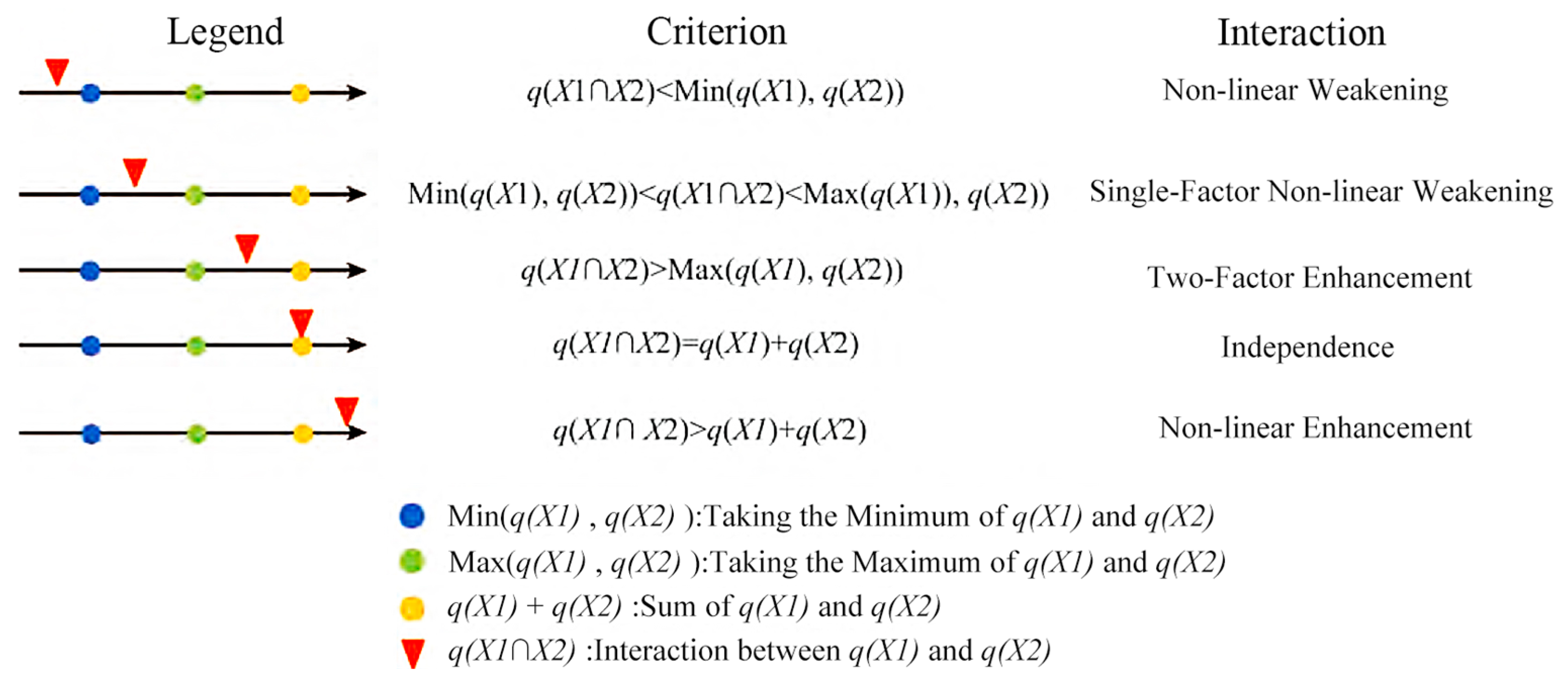
Analysis of Spatial Driving Factors—GeoDetector (GD)

The GD, proposed by Wang Jinfeng, integrates GIS spatial analysis techniques and introduces the “factor detection” metric. This method can be applied to analyze the spatial variation in variables, thus revealing possible causal connections between them [50,51]. By employing the GD, the determinant power $q$ is utilized to assess how different factors influence the spatial differentiation of urban CTL. The calculation formula for $q$ is as follows:

$$q=1-{\displaystyle \frac{1}{n{\sigma }^2}}{\sum }_{i=1}^m{n}_i{\sigma }_i^2$$

(13)

In the formula, ${\sigma }_i^2$ represents the variance of the different spatial elements, $n_i$ denotes the sample size, $i$ indicates the number of spatial variables, and ${\sigma }^2$ refers to the total variance within the region. To facilitate the calculation of the spatial distance relationships among these factors, all spatial elements are uniformly converted into 1 km × 1 km grids, and spatial proximity calculations are performed for these factors. The value range of $q$ is [0, 1]. The six spatial driving factors are presented in

Table 3. Spatial driving factors of urban CTL in the YRDUR.

Category	Spatial Driving Factors	Interpretation Variable Code
Location Space	Distance from Main Railway (km)	X18
	Distance from Main Highway (km)	X19
	Distance from Main River (km)	X20
Geographic Space	Ruggedness (°)	X21
	Slope (°)	X22
	Elevation (m)	X23

.

3. Results and Analysis

3.1. Analysis of Spatiotemporal Evolution of Land Use

3.1.1. Changes in Spatial Scale

Analyzing the spatial distribution, the land use type for YRDUR from 2000, 2005, 2010, 2015, and 2020 highlight significant shifts in land use patterns over the last twenty years. The most notable trends are the ongoing CTL expansion and the continuous Cultivated Land (hereinafter referred to as “CVL”) reduction, while the areas and proportions of other land use types have remained relatively stable. CVL, which is the largest land use type in the YRD, is extensively distributed in the northeastern plains of the region. Its spatial distribution closely aligns with the spread of CTL. Over the 20-year period, the concentration and contiguity of CVL were gradually encroached upon by CTL, significantly weakening its degree of concentration and contiguity. Forest land (hereinafter referred to as “FL”) experienced a slight decrease, whereas grassland (hereinafter referred to as “GL”), water body (hereinafter referred to as “WB”), and other land use types were dispersed spatially and showed no significant changes.

From a quantitative standpoint, the ranking of land use types by area shifted continuously between 2000 and 2020 (

Table 4. Land use area by type in the YRDUR from 2000 to 2020.

Type	2000		2005		2010		2015		2020
	Area (km2)	Proportion (%)	Area (km2)	Proportion (%)	Area (km2)	Proportion (%)	Area (km2)	Proportion (%)	Area (km2)	Proportion (%)
CVL	1.13 × 105	50.87	1.09 × 105	49.27	1.04 × 105	46.59	1.02 × 105	45.57	1.00 × 105	45.08
FL	6.55 × 104	29.51	6.53 × 104	29.42	6.49 × 104	29.15	6.48 × 104	29.1	6.46 × 104	28.98
GL	8.15 × 103	3.67	8.05 × 103	3.63	7.61 × 103	3.42	7.53 × 103	3.38	7.94 × 103	3.57
WB	1.87 × 104	8.44	1.91 × 104	8.59	2.07 × 104	9.3	2.05 × 104	9.18	1.97 × 104	8.84
CTL	1.65 × 104	7.5	2.00 × 104	9.07	2.55 × 104	11.45	2.82 × 104	12.67	2.99 × 104	13.38
UL	4.14 × 101	0.02	4.26 × 101	0.02	2.33 × 102	0.11	2.06 × 102	0.09	3.46 × 102	0.16

). In 2005, the types hierarchy by area from largest to smallest was CVL > FL > WB > CTL > GL > unused land (hereinafter referred to as “UL”). By 2020, CTL had climbed from fourth to third place, indicating consistent positive growth, while CVL experienced notable negative growth. The areas of other land types exhibited minor fluctuations. Over the two decades, CVL saw the most significant reduction, with its proportion decreasing from 50.87% to 45.08%. The declines in FL and GL were less pronounced, with their proportions dropping from 29.51% and 3.67% to 28.98% and 3.57%, respectively. The WB area initially rose and then fell, leading to a slight overall increase from 8.44% to 8.84%. CTL exhibited the largest increase, with its proportion rising from 7.50% in 2000 to 13.38% in 2020, reaching a total area of 29,855.01 km². Although the area of UL experienced significant fluctuations, its overall scale was limited, resulting in only a slight influence on the general land use pattern. Overall, the urbanization in the YRDUR continuously encroached upon agricultural and ecological spaces, underscoring the significant human–land conflict.

3.1.2. Degree of Dynamic Change

From the standpoint of the single land use dynamic degree (

Table 5. Analysis of land use dynamics in the YRDUR from 2000 to 2020.

Land Use Types	Land Use Dynamic Degree
	2000–2005	2005–2010	2010–2015	2015–2020	2000–2020
CVL	−0.632	−1.012	−0.439	−0.218	−0.553
FL	−0.057	−0.109	−0.035	−0.084	−0.071
GL	−0.266	−1.075	−0.209	1.083	−0.130
WB	0.371	1.725	−0.247	−0.752	0.258
CTL	4.203	5.333	2.131	1.131	3.960
UL	0.556	90.063	−2.526	13.803	36.762
Comprehensive Dynamic Degree	0.347	0.610	0.246	0.193	0.316

), between 2000 and 2020, there was a continuous decrease in CVL and FL. The rate of decline in CVL initially increased before declining, while the reduction rate for FL first rose, then fell, and later rose once more. CTL as a whole exhibited growth, though the growth rate steadily diminished, which was a trend associated with the YRDUR’s focus on ecological civilization and the ongoing restriction of CTL expansion. The dynamic shifts in GL and WB did not present clear patterns, showing varying rates of increase and decrease over the 20-year period. UL showed the most pronounced fluctuations due to its smaller area, where even minor changes resulted in significant proportional shifts. From the perspective of comprehensive dynamic change degree, except for the period between 2005 and 2010, when land use structure fluctuations were relatively severe, reaching 0.610, other periods maintained levels around 0.3 or lower.

3.1.3. TM Analysis

From 2000 to 2020, notable shifts occurred in the land use structure, as detailed in

Table 6. TM of land use type areas in the YRDUR from 2000 to 2020.

2000	2020
	CVL	FL	GL	WB	CTL	UL
CVL	97,663.48 km2	850.88 km2	139.88 km2	1490.72 km2	12,743 km2	28.28 km2
FL	821.92 km2	63,424.92 km2	223.92 km2	114.12 km2	846.2 km2	32.32 km2
GL	245.72 km2	183.16 km2	7081.28 km2	463.68 km2	173.52 km2	4.64 km2
WB	754.8 km2	42.40 km2	327.64 km2	16,611.60 km2	731.12 km2	224.64 km2
CTL	844.12 km2	46.48 km2	20.48 km2	622.08 km2	15,068.8 km2	7.44 km2
UL	0.72 km2	2.92 km2	0.12 km2	1.48 km2	5.16 km2	30.52 km2

and

Table 7. TM of proportion for land use type area in the YRDUR from 2000 to 2020.

2000	2020
	CVL	FL	GL	WB	CTL	UL
CVL	86.49%	0.75%	0.12%	1.32%	11.29%	0.03%
FL	1.26%	96.89%	0.34%	0.17%	1.29%	0.05%
GL	3.01%	2.25%	86.87%	5.69%	2.13%	0.06%
WB	4.04%	0.23%	1.75%	88.87%	3.91%	1.20%
CTL	5.08%	0.28%	0.12%	3.75%	90.72%	0.04%
UL	1.76%	7.14%	0.29%	3.62%	12.61%	74.58%

. Over 10% of the regions designated as CVL, GL, WB, and UL saw transitions. FL exhibited the least change, with 96.89% of its area remaining constant, preserving its overall integrity. Among the changes, 11.29% of CVL transitioned into CTL, indicating significant urban expansion encroaching on agricultural territory. FL was primarily converted to CVL and CTL but in minimal scales. GL mainly shifted to WBs, CVL, and FL, leading to a substantial overall decline in area. WBs were predominantly replaced by CTL and CVL, highlighting significant human activity encroaching on ecological spaces. The majority of CTL was transformed into CVL and WBs, while UL showed significant variability.

3.2. Analysis of LSP Spatiotemporal Evolution

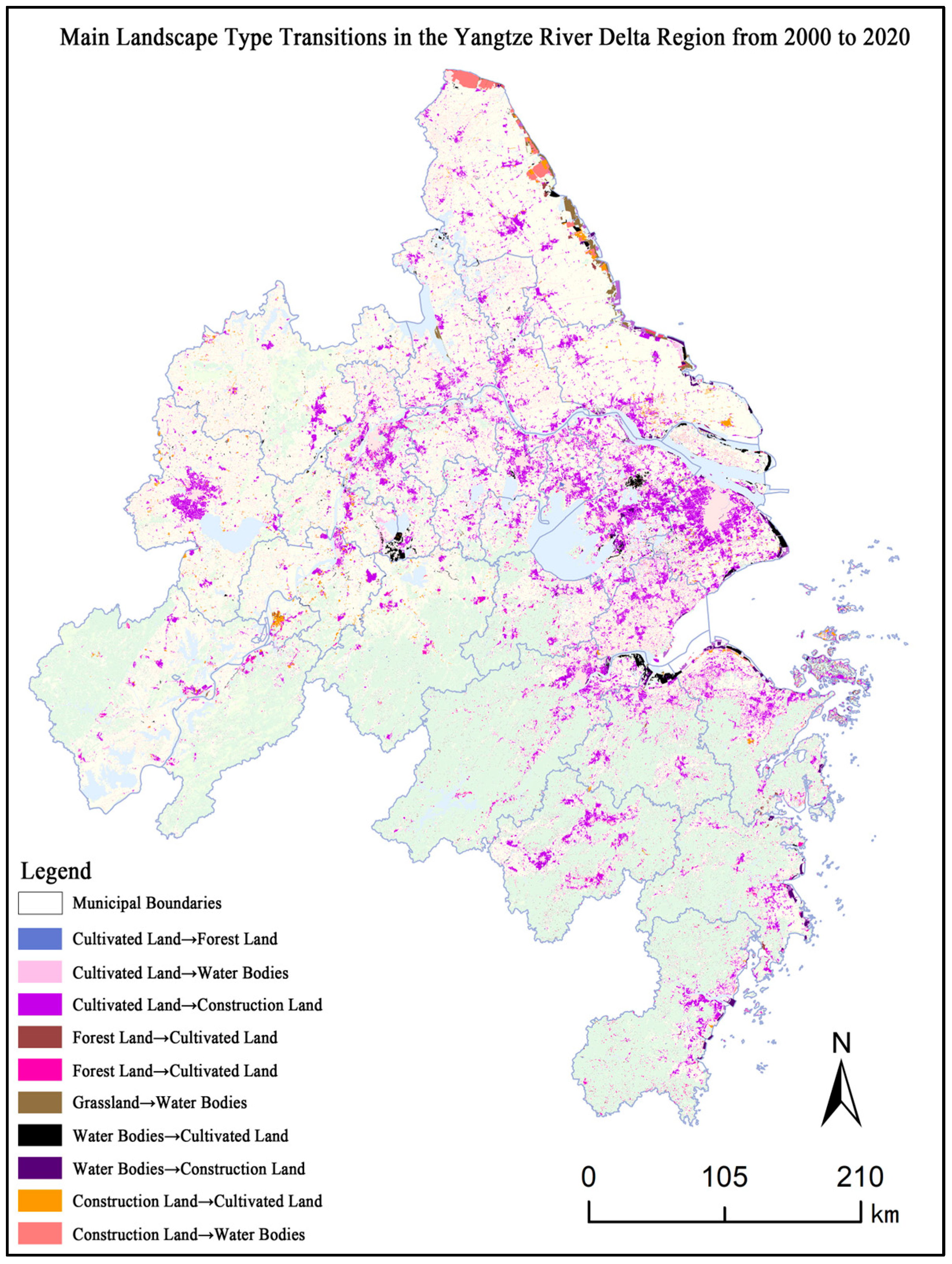
3.2.1. Spatiotemporal Distribution Patterns of Landscape Type Transitions

Building on the land use TM analysis, we determine the 10 most prevalent types of landscape transitions by volume from 2000 to 2020 and depict these transitions within the YRDUR, as illustrated in Figure 2. Over the two-decade span, landscape type transitions predominantly occurred in cities surrounding Taihu Lake and Hangzhou Bay. The most significant transition was from CVL to CTL, severely impacting agricultural areas. Further investigation reveals that the urban transition area northeast of Taihu Lake was considerably larger than that around Hangzhou Bay, particularly in cities like Shanghai, Suzhou, and Wuxi. Additionally, Hefei saw a massive scale of landscape type transition during this period, indirectly corroborating Hefei’s rapid economic growth over the 20 years, which was characterized by the persistent growth of its central urban zone and the continual encroachment into its ecological and agricultural areas. It is evident that landscape type transitions were predominantly focused in regions with advanced economic development. Conversely, the northern parts of the YRD, which had lower levels of economic development, experienced landscape transitions primarily as scattered points without forming continuous transition areas. In the southern mountainous and hilly cities of the YRD, some ecological spaces were affected by urban expansion. Ensuring the preservation and continuity of ecological areas would continue to be a significant concern for the YRDUR moving forward.

3.2.2. Changes in Overall Landscape Level

By utilizing FRAGSTATS 4.3 software, we analyze the land use landscape type maps and obtained the overall landscape-related indices for the five time intervals spanning from 2000 to 2020 (

Table 8. LSP index and calculation details.

Year	Landscape Fragmentation Index				Landscape Heterogeneity Index			Landscape Aggregation Index		Landscape Diversity Index
	NP /Count	PD /Count/100 ha	ED/ m/ha	MPS /ha	LPI /%	LSI /-	MSI /-	AI /%	CONTAG/%	SHDI /-	SHEI /-
2000	137,432	0.619	17.25	161.49	18.43	208.24	1.24	82.60	49.35	1.23	0.686
2005	135,766	0.611	17.57	163.47	18.14	211.98	1.25	82.29	48.09	1.26	0.702
2010	134,279	0.603	18.08	165.95	17.98	218.39	1.26	81.78	46.17	1.31	0.729
2015	133,538	0.599	18.07	166.86	16.80	218.27	1.27	81.79	45.73	1.32	0.736
2020	132,784	0.595	17.98	168.09	17.90	217.59	1.27	81.87	45.25	1.33	0.744

). The following discussion integrates the LSP indices to scrutinize the progression of the overall landscape level from four dimensions: the fragmentation, heterogeneity, aggregation, and diversity of landscape. The detailed analysis is as follows:

(1)

Landscape Fragmentation Analysis

Landscape fragmentation refers to the process in which a landscape transitions from a single, homogeneous, and continuous whole to a complex, heterogeneous, and discontinuous mosaic of patches due to interference from natural or human factors. Higher values of NP, PD, and ED, along with lower MPS values, indicate increased landscape fragmentation. As shown in Table 8 and

Table 9. LSP index in different land use types and calculation details.

Land Use Types	Year	Landscape Fragmentation Index				Landscape Heterogeneity Index		Landscape Aggregation Index
		NP /Count	PD /Count/100 ha	ED/ m/ha	MPS /ha	LPI /%	LSI /-	AI /%	CONTAG/%
CVL	2000	21,482	50.88	14.96	525.67	14.21	248.36	85.27	70.70
	2005	22,248	49.28	15.11	491.58	13.32	254.88	84.63	70.62
	2010	23,408	46.58	15.38	443.46	12.67	267.18	83.47	70.34
	2015	23,804	45.57	15.29	426.59	12.43	268.52	83.20	70.21
	2020	23,656	45.01	15.03	424.66	12.31	265.87	83.27	70.56
FL	2000	10,042	29.51	7.47	652.12	18.43	165.65	87.12	48.32
	2005	10,043	29.42	7.47	650.24	18.14	165.83	87.09	51.05
	2010	10,202	29.15	7.54	636.70	17.98	168.53	86.84	53.96
	2015	10,208	29.11	7.48	635.33	16.80	167.38	86.92	55.059
	2020	9938	28.98	7.54	650.74	17.90	169.12	86.76	56.21
GL	2000	9969	3.68	2.06	81.82	0.12	129.78	71.39	59.88
	2005	9644	3.63	2.04	83.53	0.11	128.98	71.40	60.44
	2010	9836	3.42	2.01	77.46	0.11	131.21	70.09	60.25
	2015	9845	3.38	1.99	76.59	0.11	130.35	70.12	60.63
	2020	10,031	3.57	2.06	79.46	0.11	132.18	70.54	63.26
WB	2000	17,711	8.43	2.79	105.68	2.13	117.32	82.96	51.21
	2005	18,121	8.59	2.92	105.23	2.07	121.49	82.52	52.95
	2010	18,777	9.30	3.04	110.37	2.09	122.11	83.15	55.82
	2015	19,289	9.19	3.08	106.18	2.05	124.19	82.75	56.42
	2020	19,365	8.88	3.07	102.31	1.86	125.46	82.29	59.29
CTL	2000	78,010	7.48	7.20	21.29	0.26	310.51	51.89	22.37
	2005	75,483	9.06	7.58	26.64	0.40	297.20	58.14	25.79
	2010	71,611	11.44	8.12	35.60	0.62	284.20	64.47	29.79
	2015	69,944	12.66	8.23	40.32	0.94	274.10	67.42	31.40
	2020	69,269	13.39	8.17	43.15	1.14	265.45	69.37	34.42
UL	2000	218	0.02	0.02	18.77	0.00	17.45	46.87	68.52
	2005	227	0.02	0.02	18.45	0.00	17.63	46.72	68.38
	2010	445	0.11	0.06	52.69	0.02	22.35	71.58	88.79
	2015	448	0.09	0.06	45.54	0.02	22.66	69.20	86.22
	2020	525	0.17	0.07	74.22	0.04	22.92	77.50	89.35

, from 2000 to 2020, the number of patches (NP) and patch density (PD) experienced a slow and gradual decline, suggesting a steady improvement in the overall landscape integrity of the YRDUR. This positive trend was primarily attributed to frequent human activities in the area, which merged some fragmented landscapes and enhanced the overall landscape cohesion. The edge density (ED) initially saw a slight increase followed by a steady decrease, with minor overall fluctuations, reflecting typical variations in national land development over the past two decades. The mean patch size (MPS) gradually rose from 161.49 ha to 168.09 ha, further indicating the integration of fragmented landscapes. In summary, over the last 20 years, the landscape fragmentation degree in the YRDUR progressively decreased. Nevertheless, the ongoing transformation of agricultural land into various other uses, particularly for construction, exacerbated fragmentation. These changes indicate that the agricultural space and related ecological space dominated by CVL were affected and squeezed by urban construction space largely driven by human development activities.

(2)

Landscape Heterogeneity Analysis

Lower LPI values, along with higher LSI and MSI values, suggest increased landscape heterogeneity. As illustrated in Table 8 and Table 9, the Largest Patch Index (LPI) initially declined and then rose from 2000 to 2020, hitting its lowest point around 2015, which indicates the peak of landscape heterogeneity, before climbing back to levels seen around 2010. Both the Landscape Shape Index (LSI) and Mean Shape Index (MSI) followed a similar pattern, peaking around 2015 and then slightly decreasing. This pattern was the inverse of the LPI changes with all three indices highlighting that landscape heterogeneity was at its highest around 2015. This transition heralded a new focus on ecological civilization and the end of ineffective land development methods. Subsequently, in May 2016, the state council’s executive meeting approved the development plan of the YRDUR, which further stressed the importance of ecological civilization construction, placing greater emphasis on protecting natural ecosystems and the environment, effectively controlling urban sprawl and curbing disorderly urban expansion. This indicates that around 2015, there was a significant shift from a relatively rough land development model to a more orderly development approach.

(3)

Landscape Aggregation Analysis

Higher AI values indicate a greater level of patch aggregation, while higher CONTAG values indicate that a leading patch type in the landscape shows significant connectivity and clustering. As depicted in Table 8 and Table 9, the AI gradually dropped from 82.60% to 81.87% between 2000 and 2020, reflecting a minor decline in patch aggregation. This demonstrates that despite relatively frequent types transitions in land use within the YRDUR, the overall aggregation of landscape patches remained largely unchanged, and the general spatial relationships of land use stayed relatively stable. Meanwhile, the Contagion Index (CONTAG) fell from 49.35% to 45.25%, reflecting a minor decline in the connectivity of patches. The relevant patches were mainly concentrated and developed in large towns in the YRD. This reduction in the connectivity and aggregation of patches was mainly linked to urban sprawl, which disrupted the flow of energy and information among species in ecological and agricultural spaces.

(4)

Landscape Diversity Analysis

Higher SHDI and SHEI values signify greater landscape type diversity and a more even spatial distribution. As illustrated in Table 8 and Table 9, the Shannon Diversity Index (SHDI) and Shannon Evenness Index (SHEI) displayed comparable evolutionary patterns from 2000 to 2020, both trending upward gradually. This reflects a continuous improvement in the balance of landscape type distribution in the YRDUR. It also implies that human development activities consistently expanded CTL, altering the LSP structure and progressively narrowing the distribution gap between landscape types.

3.3. Analysis of Evolution in Urban CTL Expansion

By examining the land use patterns evolution and LSP analysis results mentioned earlier, it is evident that the most prominent feature of land spatial evolution in the YRDUR is the relentless conversion of CVL into CTL. CTL has consistently expanded, while CVL has decreased, with other land categories experiencing only slight variations. The significant growth of CTL emerges as the primary driver of spatial changes in the region. Moving forward, it is essential to implement strict controls on the unchecked expansion of urban CTL, protect the ecological baseline, and maintain the overall balance of CVL. To establish effective spatial management strategies, the analysis of urban CTL expansion patterns and driving factors is necessary. Therefore, this study seeks to identify the patterns regarding the direction, scale, and intensity of urban CTL expansion, as well as to explore the underlying driving factors, which will inform future research on spatial conflicts and the development of a comprehensive spatial management framework.

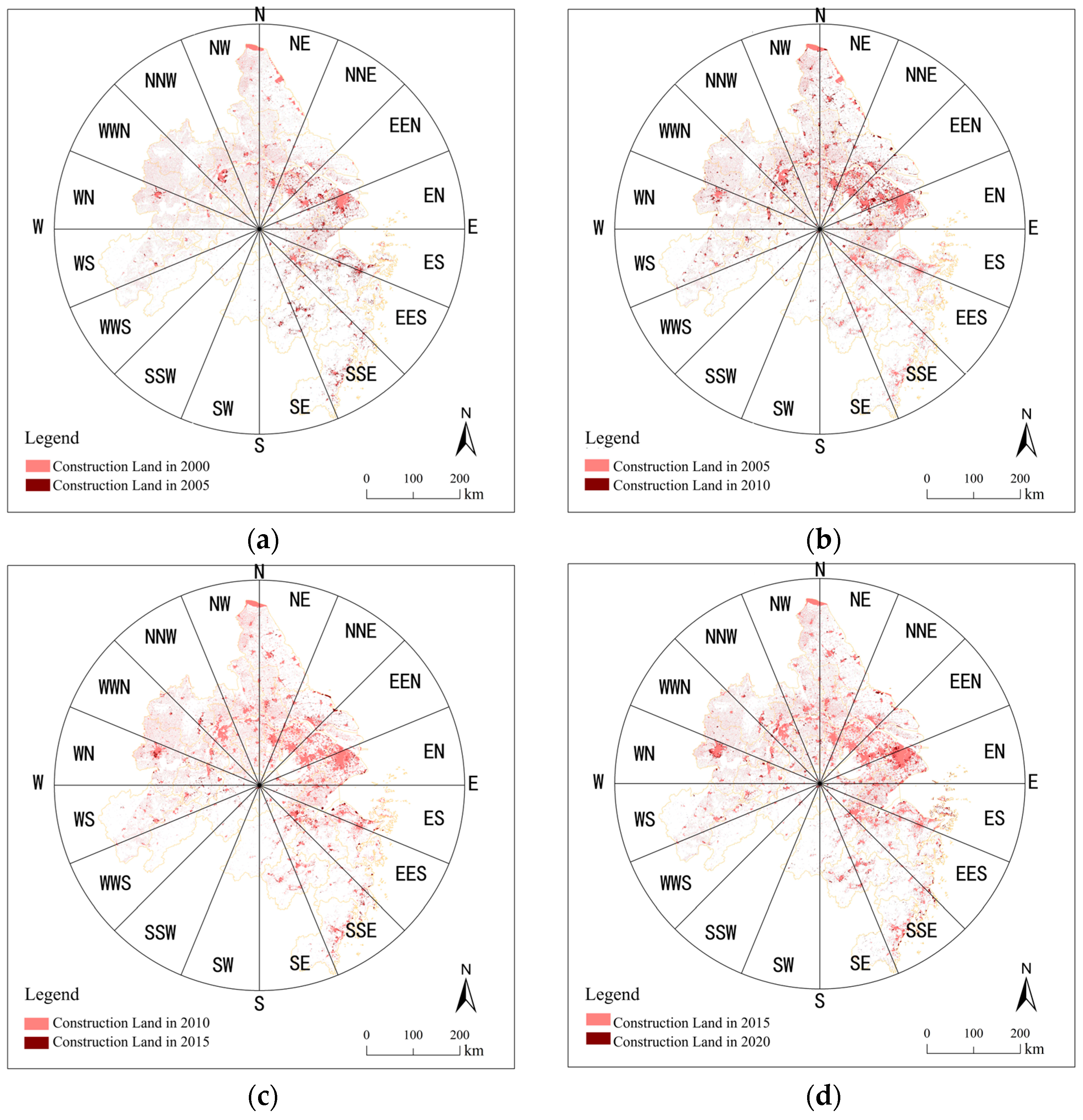
3.3.1. Direction of Urban Construction Space Expansion

(1)

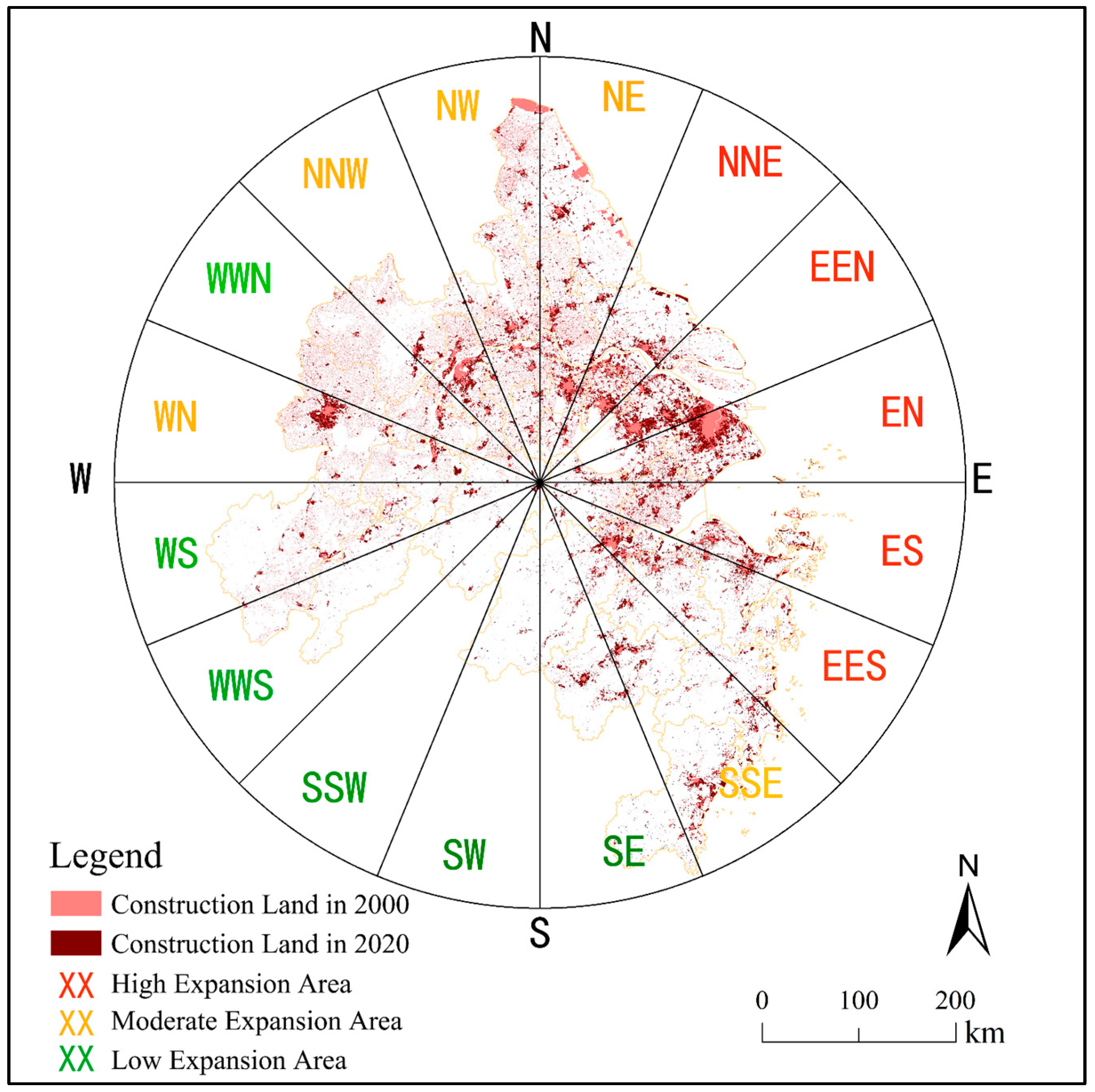
Results of SDE Analysis

Based on the calculations above, we derive the SDE for urban CTL for the years 2000, 2005, 2010, 2015, and 2020 (Figure 3). During these years, the weighted mean center of the ellipses representing urban CTL in the YRDUR consistently positioned itself to the northwest of Changzhou. The lengths of the major axes were 207.69 km, 210.91 km, 217.29 km, 216.08 km, and 220.24 km, respectively, while the lengths of the minor axes were 167.27 km, 167.59 km, 168.74 km, 168.90 km, and 170.62 km, respectively. The azimuth angles were 125.19°, 126.18°, 130.35°, 130.53°, and 132.47°, respectively. Overall, the SDE for these five periods exhibited slight movements, mainly in the northwest–southeast direction, encompassing a broad area that included most cities in the YRD. However, some southern cities, such as Wenzhou, Taizhou, and Jinhua, were not covered, clearly indicating that urban construction conditions in the central and eastern areas of the YRD were markedly superior to those in the southern region.

(2)

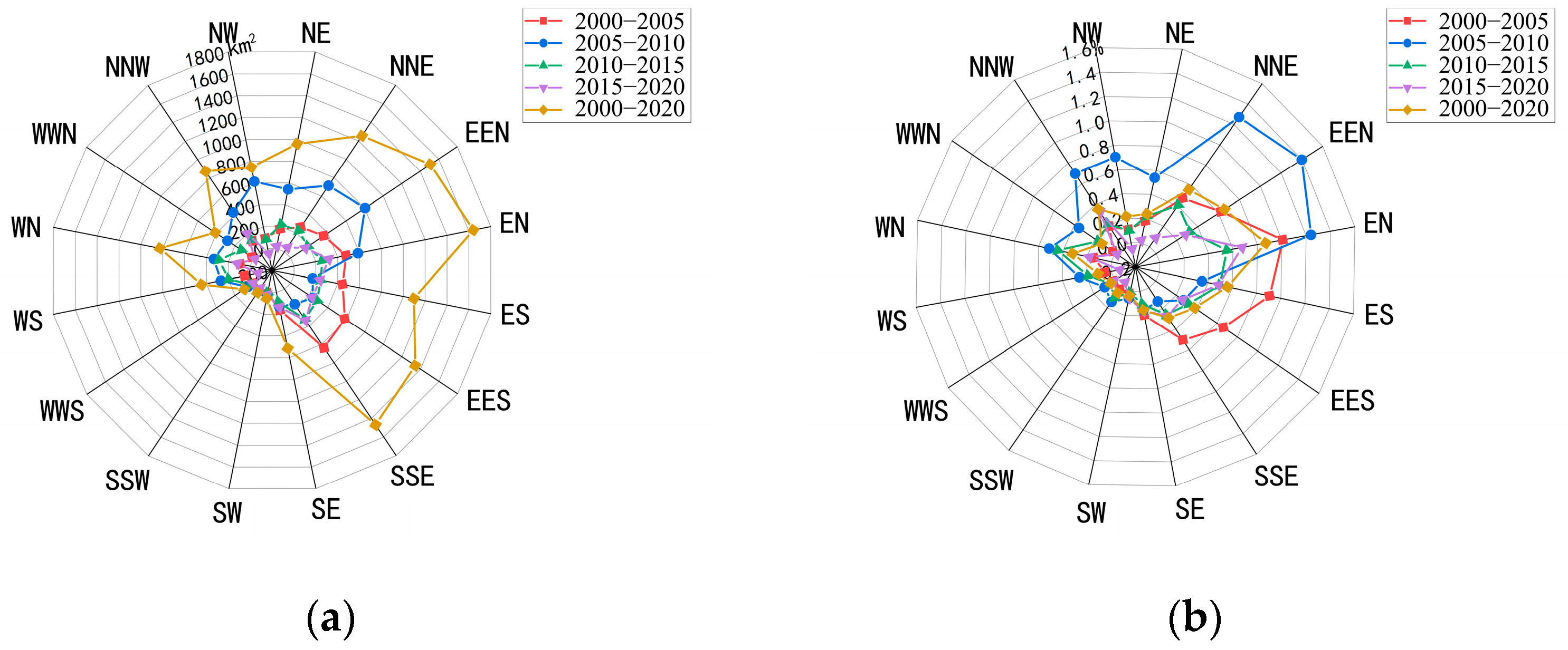
Subdivision of Urban CTL Expansion Directions Based on Equal Sector Analysis

The previous text has generally elucidated that the main direction of CTL expansion in the YRD has been oriented from the northwest to the southeast. To further clarify the expansion details, this study employs equal sector analysis to subdivide the expansion direction. Equal sector analysis is based on the core of the study area, using the furthest point as the radius to segment the region into sectors with equal areas. It then calculates the CTL expansion area within each sector to characterize the land expansion direction [52,53]. As illustrated in Figure 4, the CTL in the YRDUR reveals a fan-wing expansion pattern across four stages, predominantly oriented toward the south and southwest. Specifically, from 2000 to 2005, the expansion directions were mainly in the EN, ES, EES, and SSE sectors; from 2005 to 2010, the expansion was concentrated in the NE, NNE, EEN, and EN sectors; from 2010 to 2015, the expansion was primarily in the EN, ES, EES, and SSE sectors, with a notable trend toward the WN sector; from 2015 to 2020, the expansion continued predominantly in the EN, ES, EES, and SSE sectors.

Analyzing the results from the aforementioned four periods, it becomes clear that from 2000 to 2020, the EN direction experienced the most notable growth with CTL steadily increasing across nearly every period. The EN direction primarily encompasses Shanghai and Suzhou, which are central to the YRDUR. Throughout this 20-year span, urban CTL expansion was predominantly centered in the EEN, EN, ES, EES, and SSE directions (Figure 5). The cities in these regions, including Nantong, Suzhou, Shanghai, Jiaxing, Hangzhou, Ningbo, Taizhou, and Wenzhou, all adopt outward-oriented economic development models, exhibit high economic levels, and are continually attracting migrants. These cities face strong demands for economic development, and balancing economic growth, ecological protection, and agricultural production remains a significant challenge for them. Importantly, aside from these areas, the WN direction saw rapid CTL expansion during the 2010–2015 period, mainly including Hefei, Wuhu, and Ma’anshan, which was largely attributed to rapid urbanization and industrial upgrading in these cities.

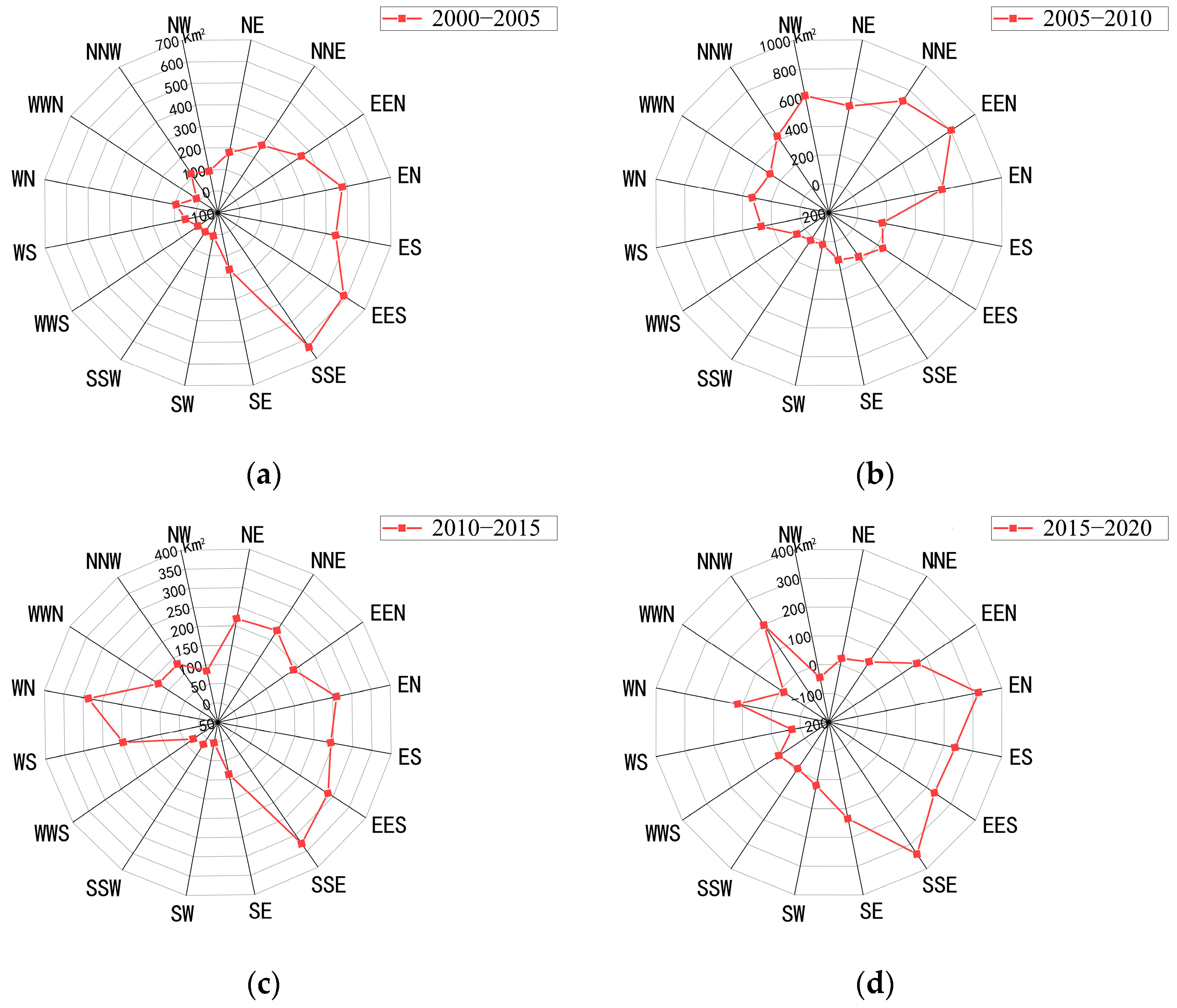
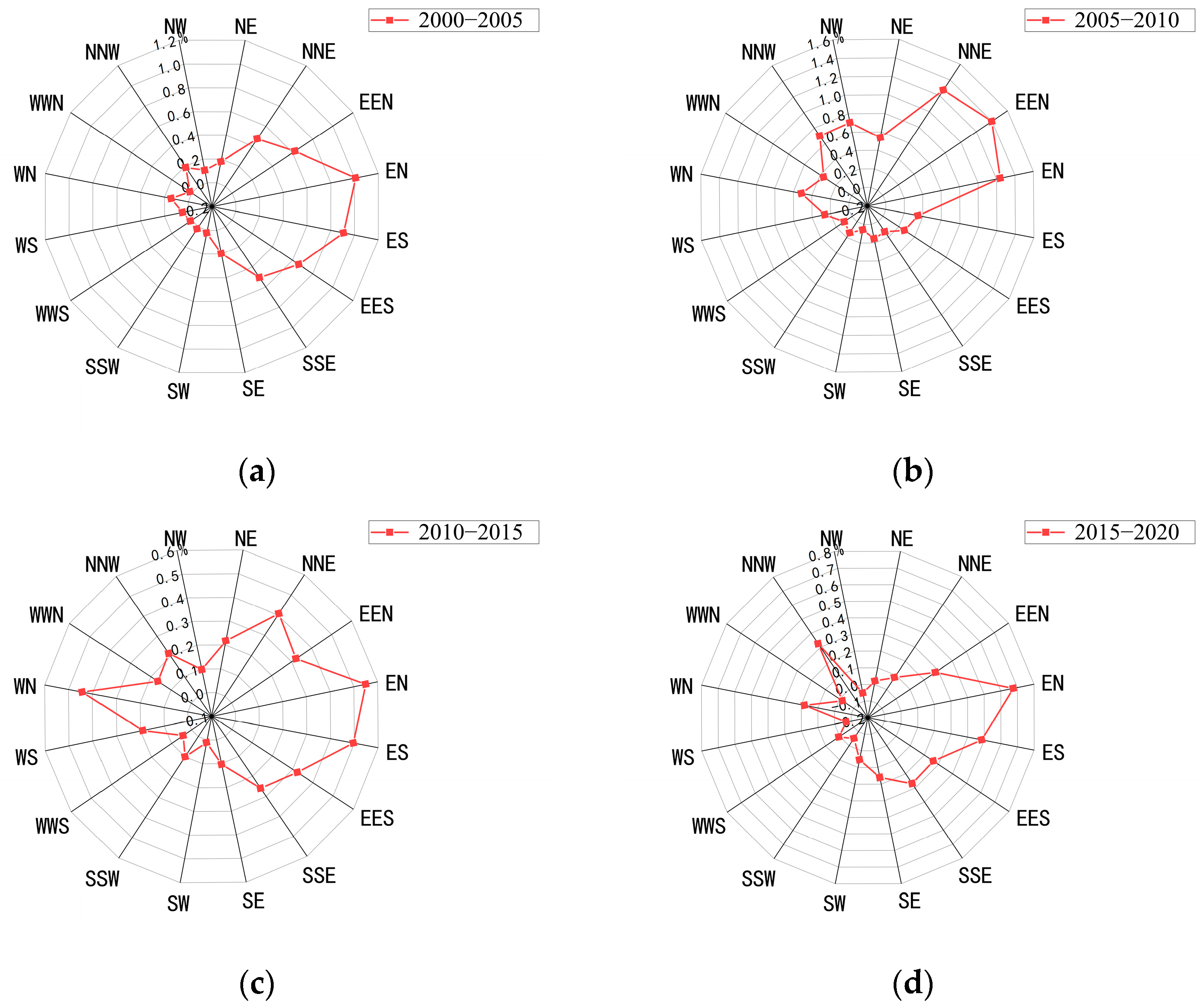
3.3.2. Scale and Intensity of Urban CTL Expansion

Through introducing indicators such as expansion area, annual average expansion area, and annual average expansion intensity, the CTL area in 16 subdivided expansion zones are assessed across different directions for each period to compare the strength, speed, and trend. This assessment reveals the scale and intensity of land expansion in these regions from 2000 to 2020. Using the natural fracture method and referring to relevant literature and planning policies, the classification of expansion intensity is represented by the annual average expansion intensity index over a span of 20 years. The classifications are defined as follows: 0–0.15% for low-intensity expansion, 0.15–0.36% for medium-intensity expansion, and 0.36–0.87% for high-intensity expansion with specific calculation details provided in

Table 10. Analysis of scale and intensity of CTL expansion in the YRDUR (2000–2020).

Sector	Time Period	Expansion Area (km2)	Annual Average Expansion Area (km2/Year)	Annual Average Expansion Intensity (%)	Expansion Intensity Classification
NE	2000–2005	179.08	35.82	0.18	Medium-Intensity Expansion
	2005–2010	540.75	108.15	0.54
	2010–2015	218.73	43.75	0.22
	2015–2020	21.37	4.27	0.02
	2000–2020	959.92	48.00	0.24
NNE	2000–2005	265.06	53.01	0.47	High-Intensity Expansion
	2005–2010	712.45	142.49	1.27
	2010–2015	228.41	45.68	0.41
	2015–2020	47.46	9.49	0.09
	2000–2020	1253.37	62.67	0.56
EEN	2000–2005	358.40	71.68	0.62	High-Intensity Expansion
	2005–2010	803.90	160.78	1.40
	2010–2015	185.42	37.08	0.32
	2015–2020	161.07	32.21	0.28
	2000–2020	1508.79	75.44	0.66
EN	2000–2005	476.66	95.33	1.01	High-Intensity Expansion
	2005–2010	585.74	117.15	1.24
	2010–2015	259.85	51.97	0.55
	2015–2020	318.99	63.80	0.68
	2000–2020	1641.24	82.06	0.87
ES	2000–2005	445.22	89.04	0.91	High-Intensity Expansion
	2005–2010	170.94	34.19	0.35
	2010–2015	243.09	48.62	0.50
	2015–2020	238.02	47.60	0.49
	2000–2020	1097.27	54.86	0.56
EES	2000–2005	584.63	116.93	0.66	High-Intensity Expansion
	2005–2010	240.44	48.09	0.27
	2010–2015	285.17	57.03	0.32
	2015–2020	232.61	46.52	0.26
	2000–2020	1342.85	67.14	0.38
SSE	2000–2005	637.95	127.59	0.51	Medium-Intensity Expansion
	2005–2010	163.89	32.78	0.13
	2010–2015	326.51	65.30	0.26
	2015–2020	340.01	68.00	0.27
	2000–2020	1468.36	73.42	0.29
SE	2000–2005	164.41	32.88	0.20	Low-Intensity Expansion
	2005–2010	129.78	25.96	0.16
	2010–2015	86.00	17.20	0.10
	2015–2020	135.04	27.01	0.16
	2000–2020	515.23	25.76	0.15
SW	2000–2005	8.09	1.62	0.02	Low-Intensity Expansion
	2005–2010	21.68	4.34	0.06
	2010–2015	4.04	0.81	0.01
	2015–2020	20.24	4.05	0.05
	2000–2020	54.05	2.70	0.04
SSW	2000–2005	3.78	0.76	0.02	Low-Intensity Expansion
	2005–2010	24.90	4.98	0.14
	2010–2015	17.88	3.58	0.10
	2015–2020	−9.35	−1.87	−0.05
	2000–2020	37.21	1.86	0.05
WWS	2000–2005	8.74	1.75	0.01	Low-Intensity Expansion
	2005–2010	61.48	12.30	0.10
	2010–2015	26.33	5.27	0.04
	2015–2020	3.90	0.78	0.01
	2000–2020	100.45	5.02	0.04
WS	2000–2005	49.61	9.92	0.05	Low-Intensity Expansion
	2005–2010	269.48	53.90	0.26
	2010–2015	197.19	39.44	0.19
	2015–2020	−72.08	−14.42	−0.07
	2000–2020	444.21	22.21	0.11
WN	2000–2005	92.25	18.45	0.14	Medium-Intensity Expansion
	2005–2010	330.77	66.15	0.51
	2010–2015	285.77	57.15	0.44
	2015–2020	116.14	23.23	0.18
	2000–2020	824.93	41.25	0.32
WWN	2000–2005	15.93	3.19	0.02	Low-Intensity Expansion
	2005–2010	281.24	56.25	0.35
	2010–2015	130.71	26.14	0.17
	2015–2020	−15.72	−3.14	−0.02
	2000–2020	412.16	20.61	0.13
NNW	2000–2005	115.09	23.02	0.19	Medium-Intensity Expansion
	2005–2010	425.97	85.19	0.70
	2010–2015	130.97	26.19	0.21
	2015–2020	197.90	39.58	0.32
	2000–2020	869.94	43.50	0.36
NW	2000–2005	92.38	18.48	0.11	Medium-Intensity Expansion
	2005–2010	613.01	122.60	0.70
	2010–2015	84.10	16.82	0.10
	2015–2020	−44.69	−8.94	−0.05
	2000–2020	744.80	37.24	0.21

.

For visual representation of the expansion, the study area is segmented into 16 sectors, each with equal angles and areas. Radar charts (Figure 6 and Figure 7) are used to calculate and depict the actual expansion area and intensity for each sector. Between 2000 and 2005, the most notable expansion occurred in the SSE direction, covering 637.95 km² with an annual growth of 127.59 km², which was followed by the EES direction. The overall expansion trend decreased counterclockwise from the SSE direction. The EN sector exhibited the highest expansion intensity at 1.01% with the western region of the YRDUR showing significantly greater expansion intensity compared to other sectors. From 2005 to 2010, the EEN and NNE directions had the largest expansion areas, measuring 803.90 km² and 712.45 km², respectively, with annual expansions of 160.78 km² and 142.49 km². The EEN sector also had the highest expansion intensity at 1.40%, the peak level over the 20-year period, indicating a strong correlation between expansion area and intensity with the overall trend more pronounced in the northeast of the YRDUR. During 2010 to 2015, the southeast direction demonstrated a notable expansion trend with the SSE direction having the most extensive expansion area, though at a lower intensity. Additionally, the WN direction saw explosive growth, marking the fastest increase in CTL area over the 20 years. From 2015 to 2020, the expansion areas in the SSE, EES, ES, and EN directions of the YRDUR were roughly the same and at a higher level but with notable differences in expansion intensity. The EN direction had an intensity of 0.68%, which was significantly higher than the ES, EES, and SSE directions.

Analyzing the radar charts that illustrate the scale and intensity of CTL expansion across four distinct periods (Figure 8) reveals that the urban CTL growth in the YRDUR from 2000 to 2020 can be categorized into phases of rapid expansion and periods of slower growth.

The rapid expansion phases occurred in 2000–2005 and 2005–2010 with both the extent and intensity of CTL growth markedly surpassing those observed in 2010–2015 and 2015–2020. During 2000–2005, the expansion scale in the SSE and EES directions was notably greater than in other directions, whereas the highest expansion intensities were primarily in the EN and ES directions. However, the high expansion scale in EES and SSE did not correspond to high intensity. From 2005 to 2010, the overall scale and intensity of CTL expansion in the YRDUR peaked over the 20 years, particularly in the northeast directions, including NNE, EEN, and EN, with the EEN direction showing the most pronounced expansion. The slow development periods spanned from 2010 to 2015 and 2015 to 2020. From 2010 to 2015, while the intensity of land expansion reduced, the directions of expansion diversified. Although the expansion area was relatively uniform across different directions, EN, ES, and NNE directions exhibited higher expansion intensities. From 2015 to 2020, there was a clear trend of parallel expansion in multiple areas toward the southwest, with a significant slowdown in land expansion in the northwest region of the YRDUR, and the overall expansion intensity was markedly below the average level over the 20 years, although the EN direction maintained a higher intensity level.

During the last two decades, the primary expansion directions of CTL in the YRDUR were toward the east and southeast, including the NNE, EEN, EN, ES, EES, and SSE directions. Among these, the EN direction accumulated the largest expansion area of 1641.24 km², which is the core area of the YRD with substantially higher economic development levels than other regions. In the southwest of the YRDUR, an important ecological conservation area, economic activities were strictly limited, resulting in minimal land expansion. In contrast, the northwest and northern regions of the YRDUR saw more restrained land expansion, which was largely because the central area attracted economic, population, and other influences away from these surrounding areas.

3.4. Analysis of Driving Factors of CTL Evolution in the YRDUR

3.4.1. Regional Division of Urban CTL Expansion Types

From the preceding analysis, a pivotal conclusion surfaces: the growth of urban CTL stands as the most significant indication of territorial space evolution in the YRDUR, and it serves as its primary driving force. This study examines the patterns of territorial space evolution in the YRD by focusing on urban CTL expansion, bearing both scientific and practical relevance. It should be highlighted that there is a notable spatial heterogeneity in the economic development levels within the region; the eastern areas surpass the western ones, and the southern regions outperform the northern ones, with certain internal areas having strong economic ties that form various metropolitan areas, including the Shanghai and Hangzhou metropolitan regions to the east, the Nanjing metropolitan area in the north–central part, and the Hefei metropolitan area to the west. This study’s regional classification method deviates from conventional studies that regroup and classify all cities within a region based on each city’s expansion intensity. Such methods often neglect the socioeconomic connections between cities within the same spatial direction. Therefore, this study suggests that the division of regions with varying expansion intensities should be considered from an integrated regional perspective, categorized by spatial direction, emphasizing the differences among various spatial directions in the YRD, while considering the interactions between cities within the same directional region. This indicates that the expansion intensity is not uniform across all cities within the region, and disparities still exist among cities within the same type of area, such as Shaoxing and Zhoushan in the high-intensity expansion area, where the CTL expansion intensity is lower than that of Hefei in the medium-intensity expansion area.

Based on the aforementioned classification approach, this study incorporates the results from the analysis of expansion intensity indices for each spatial direction previously discussed. It divides the YRDUR into areas of high, medium, and low expansion intensity, specifying their spatial locations. Figure 9 illustrates the spatial classification of 27 cities within the YRD.

The high-intensity expansion zone encompasses nine cities, primarily situated around the Yangtze River Estuary, excluding Hangzhou and Shaoxing, which are all part of the Shanghai Metropolitan Area. Serving as the central node of the premier urban agglomeration in the YRD, Shanghai boasts advanced economic development and frequent human activities, leading to significant scale effects in CTL. The medium-intensity expansion zone comprises 12 cities, which are mainly provincial capitals or economically robust cities in Anhui, Jiangsu, and Zhejiang. These cities possess stable economic foundations and vibrant commercial environments, making them attractive to large corporations and exceptional talent. Meanwhile, the low-intensity expansion zone includes six cities within Anhui Province, which are primarily tasked with agricultural production and ecological conservation. The emphasis here is on coordinating agricultural spatial patterns and maintaining ecosystem functions. Due to geographical constraints, these cities mainly adopt an inward-looking economic model, resulting in less pronounced land expansion.

3.4.2. Analysis of Spatiotemporal Driving Factors in CTL Expansion

The previous sections have already clarified that from 2000 to 2020, the YRDUR was categorized into three types of CTL evolution areas: high expansion, moderate expansion, and low expansion. Preliminary tests on the data indicate that changes over five-year intervals were not significantly noticeable. Hence, this study further simplifies the five time slices from 2000 to 2020 into three time slices: 2000, 2010, and 2020, for examining the spatiotemporal driving forces. Consequently, the adopted approach for assessing the spatiotemporal drivers of land space evolution in the YRD involves categorizing the area into three distinct CTL expansion types, and the study separately identifies the spatiotemporal driving factors for these three categories (27 cities) at the three time slices of 2000, 2010, and 2020.

In examining the spatiotemporal driving factors of CTL expansion in the YRD, we discard the traditional method of discussing spatiotemporal factors on the same dimension, which tends to obscure the distinctions between time and space and ignores the spatial heterogeneity of spatial factors. This study innovatively proposes the division of driving factors into temporal driving factors and spatial driving factors, conducting categorized analyses accordingly. Temporal driving factors are highly dynamic and include technological level, socioeconomic status, industrial structure, environmental and cultural factors, and transportation facilities. These factors showed significant variations across different time slices. Spatial factors exhibited considerable spatial heterogeneity and primarily include slope, elevation, ruggedness, distance from major roads, railways and rivers. These factors remained largely unchanged across different time slices. Consequently, the upcoming sections will first present individual quantitative analyses of temporal and spatial drivers, and then it will offer an in-depth qualitative discussion to examine the patterns influencing CTL expansion.

(1)

Analysis of Temporal Factor-Driven Results

In this study, multivariate linear stepwise regression is employed to remove collinear factors from an initial set of 28 factors, ultimately identifying 17 key drivers influencing urban construction space expansion in the YRD. Regression analysis is conducted on nine scenarios, covering high, medium, and low expansion intensity areas for the years 2000, 2010, and 2020. The findings reveal that all 17 selected temporal driving factors had significant correlations with urban CTL expansion, resulting in the formation of nine regression models (

Table 11. Regression model analysis results of temporal driving factors of urban CTL in the YRDUR.

Year	Type	Factor Type	p Value	Correlation Coefficient	Regression Model	Driving Type
2000	Low-Intensity Expansion Area	Technological Development	0.000	0.952 ***	Y = 171.497 + 18.746 × 1	Single Factor
	Medium-Intensity Expansion Area	Industrial Structure	0.000	−0.900 ***	Y = 4541.619 − 74.298 × 8	Single Factor
	High-Intensity Expansion Area	Socioeconomic, Environmental Humanities	0.001	0.897 **/−0.564 *	Y = 410.722 + 0.134 × 6 − 474.532 × 14	Dual Factors
2010	Low-Intensity Expansion Area	Socioeconomic	0.003	0.908 **/0.773 *	Y= −240.819 + 52.685 × 5 + 4.570 × 4	Dual Factors
	Medium-Intensity Expansion Area	Technological Development, Socio-economic, Industrial Structure	0.000	0.793 ***/−0.773 ***/0.472 *	Y = 1905.551 + 12.890 × 1 − 41.705 × 10 − 25.539 × 5	Multiple Factors
	High-Intensity Expansion Area	Socioeconomic, Environmental Humanities	0.000	0.919 ***/−0.577 *	Y = 301.941 + 0.121 × 6 − 857.297 × 14	Dual Factors
2020	Low-Intensity Expansion Area	Industrial Structure, Environmental Humanities, Transportation Facilities	0.000	0.988 ***/0.462 */0.512 *	Y= −2537.241 + 0.099 × 17 + 40.429 × 8 + 19.952 × 12	Multiple Factors
	Medium-Intensity Expansion Area	Technological Development	0.003	0.769 ***	Y= −560.616 + 169.980 × 1	Single Factor
	High-Intensity Expansion Area	Socioeconomic, Environmental Humanities	0.000	0.896 ***/0.884 ***/−0.598 *	Y = 376.045 + 0.095 × 7 + 0.114 × 6 − 544.779 × 14	Multiple Factors

Note: *, **, *** indicate significance levels of 0.1, 0.05, and 0.01, respectively.

).

Table 12. Temporal dominant driving factors and correlation coefficients of urban CTL in the YRDUR.

Year	Region Type	Dominant Driving Factor	Correlation Coefficient	Constant	Unstandardized Coefficient	Standardized Coefficient	Adjusted R2	D-W Test
2000	Low-Intensity Expansion Area	Percentage of Green Inventions in Total Annual Regional Invention Applications	0.952 ***	171.497	18.746	0.982	0.957	2.734
	Medium-Intensity Expansion Area	Proportion of Secondary Industry Value Added to GDP	−0.900 ***	4541.619	−74.298	−0.9	0.790	1.956
	High-Intensity Expansion Area	Number of Large-Scale Industrial Enterprises	0.897 **	410.722	0.134	0.800	0.870	2.060
		Forest Coverage Rate	−0.564 *		−474.532	−2.455
2010	Low-Intensity Expansion Area	Area of Land Requisitioned in the Current Year	0.908 **	−240.819	52.685	0.699	0.963	1.733
		Local Fiscal General Budget Expenditure	0.773 *		4.570	0.444
	Medium-Intensity Expansion Area	Percentage of Green Inventions in Total Annual Regional Invention Applications	0.793 ***	1905.551	127.890	0.834	0.867	2.387
		Proportion of Secondary Industry Employment	−0.773 ***		−41.705	−0.597
		Area of Land Requisitioned in the Current Year	0.472		−25.539	−0.463
	High-Intensity Expansion Area	Number of Large-Scale Industrial Enterprises	0.919 ***	301.941	0.121	0.820	0.926	0.773
		Forest Coverage Rate	−0.577		−857.297	−0.330
2020	Low-Intensity Expansion Area	Highway Freight Volume	0.988 ***	−2537.241	0.099	0.892	1.000	1.821
		Proportion of Secondary Industry Value Added to GDP	0.462		40.429	0.175
		Per Capita Park Green Area	0.512		19.952	0.075
	Medium-Intensity Expansion Area	Percentage of Green Inventions in Total Annual Regional Invention Applications	0.769 ***	−560.616	169.980	0.769	0.551	2.388
	High-Intensity Expansion Area	Total Retail Sales of Consumer Goods	0.896 ***	376.045	0.095	0.556	0.994	1.991
		Number of Large-Scale Industrial Enterprises	0.884 ***		0.114	0.432
		Forest Coverage Rate	−0.598 *		−544.779	−0.193

Note: *, **, and *** indicate significance levels of 0.1, 0.05, and 0.01, respectively.

displays the key driving factors for each model along with their correlation coefficients with all p-values indicating significance at below 0.05. One adjusted R2 value is measured at 0.551, while the others are approximately 0.8 or higher, indicating a strong alignment between the regression models and the actual sample data.

In 2000, the dominant temporal driving factor in low-intensity expansion regions was technological advancement. The corresponding driving factor was the percentage of green inventions in the total annual patent applications in the region (X1), which showed a positive correlation and was influenced by a single factor. In medium-intensity expansion regions, the dominant temporal driving factor was the industrial structure. The key driving factor was the proportion of added value (2nd Industry) to GDP (X8), which showed a negative correlation and was impacted by a singular element. In high-intensity expansion regions, the dominant temporal driving factors were socioeconomic and environmental–humanistic conditions. The corresponding driving factors were the number of large-scale industrial enterprises (X6) and the forest coverage rate (X14), with the former being positively correlated and the latter negatively correlated, driven by dual factors.

In the context of the YRD’s development in 2000, areas with low-intensity expansion were mainly found in the southwestern hilly and mountainous parts of the delta, emphasizing green development concepts, with urban CTL expansion largely supporting ecological and green industries. Medium-intensity expansion areas in the YRD included both economically developed regions and economically lagging regions in the north. The former was transitioning from secondary to tertiary industries during this period, while the latter were in a phase of secondary industry expansion, albeit at a lower scale than the former, resulting in an overall negative correlation. Additionally, due to ecological protection requirements, there was a negative correlation with forest coverage rates.

In 2010, the dominant temporal driving factors in regions of low-intensity expansion were socioeconomic, illustrated by local fiscal general budget expenditures (X4) and the land area requisitioned that year (X5), both showing positive correlations, thus forming a dual-factor drive. For medium-intensity expansion regions, the dominant temporal driving factors included technological development, socioeconomic status, and industrial structure, which were represented by the percentage of green inventions in the total annual patent applications (X1), the land area requisitioned that year (X5), and the proportion of secondary industry employees (X10). These factors had positive, positive, and negative correlations, respectively, indicating a multifactorial drive. In high-intensity expansion regions, the dominant temporal driving factors were socioeconomic and environmental–humanistic, which were depicted by the forest coverage rate (X14). The first factor showed a positive correlation, whereas the second exhibited a negative correlation, suggesting a dual-factor influence.

Taking into account the real development in the YRD in 2010, the expansion of urban CTL in low-intensity growth areas saw a significant increase. This was linked to the rise in local fiscal general budget expenditures and the land requisitioned by various cities that year with economic growth becoming a primary development objective during this period. Within the medium-intensity expansion areas, urban development exhibited notable variation. The southern region had largely completed its industrial transformation, emphasizing ecological protection. Conversely, northern cities were in the early stages of their industrial transformation, with a general decline in the proportion of secondary industry employees and rapid economic growth, as evidenced by a significant increase in the area of land requisitioned. In high-intensity expansion areas, the factors driving the urban CTL expansion remained consistent, showing a strong correlation with the number of large-scale industrial enterprises and forest coverage rates.

In 2020, the dominant temporal driving factors in low-intensity expansion areas included industrial structure, environmental–humanistic factors, and transportation facilities. In medium-intensity expansion areas, the dominant temporal driving factor was technological development, represented by the percentage of green inventions in the total annual patent applications in the region (X1), with a positive correlation, indicating a single-factor drive. In high-intensity expansion areas, the dominant temporal driving factors were socioeconomic and environmental–humanistic conditions, indicating a multifactorial drive.

Drawing from the actual development in the YRD as of 2020, regions with low-intensity expansion experienced notable improvements in transportation infrastructure and a significant rise in highway freight volumes, which led to a boost in urban economic growth in the area. Additionally, the share of the secondary industry grew, and per capita green park space increased, as enhanced transportation conditions unlocked the development potential of the region. After two decades of growth, the medium-intensity expansion areas in the YRD essentially completed their industrial transformation, emphasizing the development of green technology industries and promoting green development principles, which significantly minimized the disparities in development models across the region. In high-intensity expansion areas, the urban CTL expansion was strongly linked to the presence of large-scale industrial enterprises and forest coverage rates. Compared to the previous periods, there was a rise in the total retail sales of consumer goods, indicating that higher economic development levels further improved the quality of urban CTL expansion.

(2)

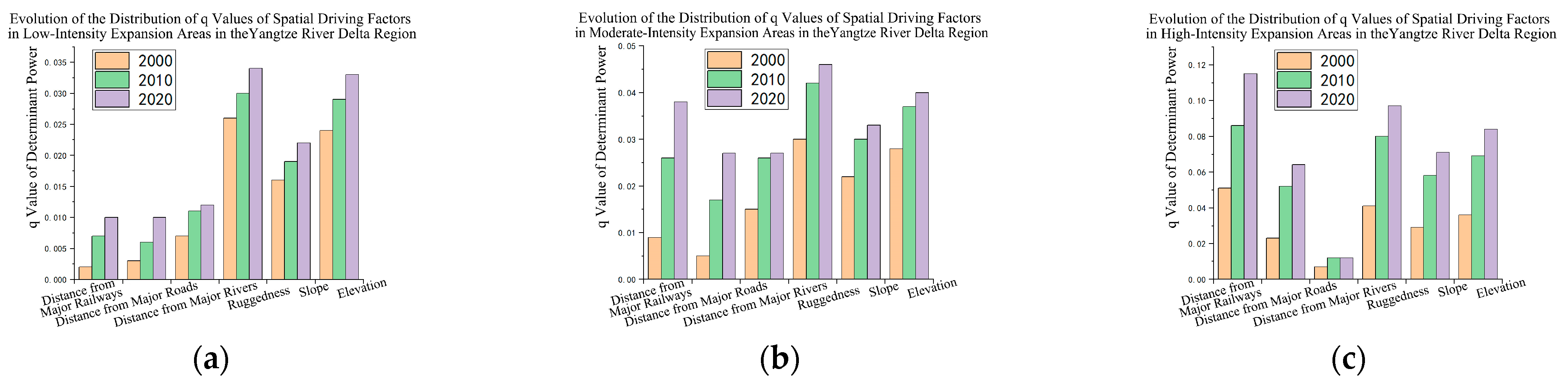
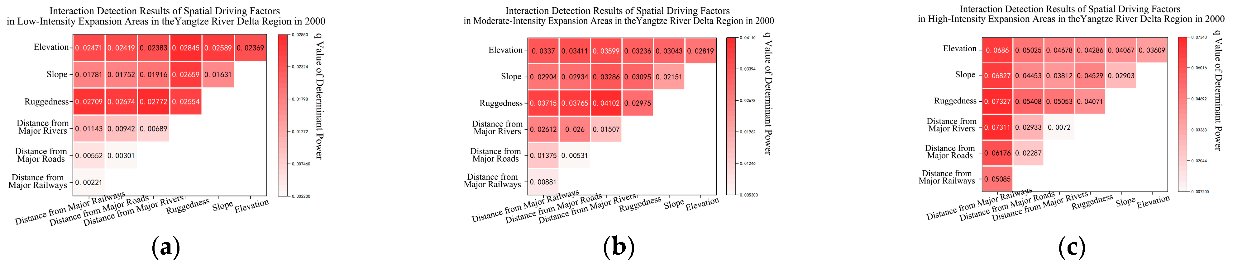
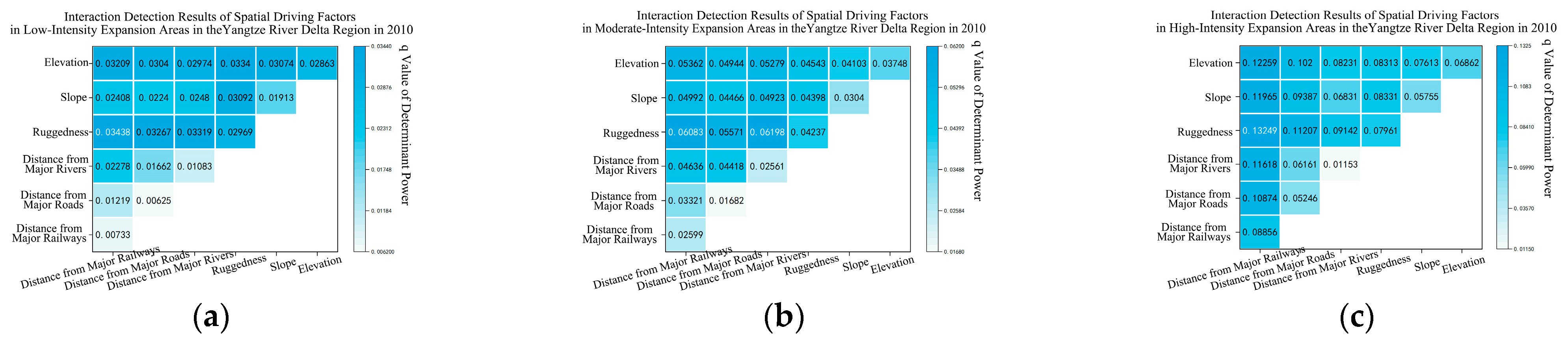
Analysis of Spatial Factor-Driven Results

In this study, urban CTL scales for the years 2000, 2010, and 2020 are employed as the dependent variable, which are spatially discretized for each of the specified time periods. Furthermore, variables including distance from major railways (X18), distance from major highways (X19), distance from major rivers (X20), ruggedness (X21), slope (X22), and elevation (X23) are spatially classified and visualized (Figure 10). These factors are then spatially associated with the discretized urban CTL data. The calculations are executed using GD software in Excel, following the procedures outlined in the relevant literature [54,55], to derive results from both factor detection and interaction detection.

Factor Detection Results: All variables meet the 0.05 significance level requirement. A static analysis of the factor detection outcomes for distinct time slices (

Table 13. Single-factor determinant q-value of spatial driving factors of urban CTL in the YRDUR.

Spatial Element	2000			2010			2020
	Low-Intensity Expansion Area	Medium-Intensity Expansion Area	High-Intensity Expansion Area	Low-Intensity Expansion Area	Medium-Intensity Expansion Area	High-Intensity Expansion Area	Low-Intensity Expansion Area	Medium-Intensity Expansion Area	High-Intensity Expansion Area
Distance from Major Railway (X18)	0.002	0.009	0.051	0.007	0.026	0.086	0.01	0.038	0.115
Distance from Major Highway (X19)	0.003	0.005	0.023	0.006	0.017	0.052	0.01	0.027	0.064
Distance from Major River (X20)	0.007	0.015	0.007	0.011	0.026	0.012	0.012	0.027	0.012
Relief Degree (X21)	0.026	0.030	0.041	0.030	0.042	0.080	0.034	0.046	0.097
Slope (X22)	0.016	0.022	0.029	0.019	0.030	0.058	0.022	0.033	0.071
Elevation (X23)	0.024	0.028	0.036	0.029	0.037	0.069	0.033	0.040	0.084

, Figure 11) indicates that the influence of factors in 2000, 2010, and 2020 is consistently distributed across various types of areas. In low-intensity expansion areas, the primary influencing factors are ruggedness (X21), elevation (X22), and slope (X23), significantly surpassing other factors. This highlights that geographic features such as terrain play a crucial role in urban CTL in these regions. In medium-intensity expansion areas, the main influencing factors are ruggedness (X21), elevation (X23), and slope (X22). The geographic environment’s influence remains substantial with the factors of distance from major railways (X18) and major rivers (X20) showing a considerable increase compared to low-intensity expansion areas. In high-intensity expansion areas, the primary influencing factors are distance from major railways (X18), ruggedness (X21), and elevation (X23).

This study modifies statistical methods to further investigate the dynamic evolution of regions with varying expansion intensities from 2000 to 2020 (Figure 12). In areas of low-intensity expansion, over the past 20 years, the impact of all spatial driving factors grew with the distance from major railways showing the most significant increase (X18). Conversely, the increase in geographic environmental factors such as ruggedness (X21), elevation (X23), and slope (X22) was relatively minor, suggesting a stable state. It is evident that for regions constrained by geographical environments, enhancing external transportation is vital for improving urban construction levels. In medium-intensity expansion areas, the influence of all spatial driving factors grew over the 20 years, with the most substantial increase in the factor of distance from major highways (X19), which was followed by the distance from major railways (X18). In high-intensity expansion areas, all spatial driving factors saw an increase in influence over the 20 years, with significant increases in all factors except for the factor of distance from major rivers (X20).

Interaction Detection Results: The main role of the interaction detector is to analyze how different risk factors interact, determining whether their joint impact increases or decreases the explanatory power, or if they influence it separately [50]. The interaction determinative power of two factors is denoted as q(X1∩X2) with the decision relationship illustrated in Figure 13. This research utilizes GD software to calculate factor interactions across different types of areas for the years 2000, 2010, and 2020.

In 2000, within the YRD’s low-intensity expansion areas, the leading three interaction determinative power (q) values for spatial driving factors influencing urban CTL were elevation (X23) ∩ ruggedness (X21), ruggedness (X21) ∩ distance from major rivers (X20), and ruggedness (X21) ∩ distance from major railways (X18), all exhibiting dual-factor enhancement relationships (Figure 14). For medium-intensity expansion areas, the top three interaction determinative power (q) values were ruggedness (X21) ∩ distance from major rivers (X20), ruggedness (X21) ∩ distance from major highways (X19), and ruggedness (X21) ∩ distance from major railways (X18). In high-intensity expansion areas, the foremost interaction determinative power (q) values were ruggedness (X21) ∩ distance from major railways (X18), distance from major rivers (X20) ∩ distance from major railways (X18), and elevation (X23) ∩ distance from major railways (X18).

In 2010, within low-intensity expansion areas, the top three interaction determinative power (q) values for spatial driving factors of urban CTL were ruggedness (X21) intersecting with distance from major railways (X18), elevation (X23) intersecting with ruggedness (X21), and ruggedness (X21) intersecting with distance from major rivers (X20), all exhibiting dual-factor enhancement (Figure 15). For medium-intensity expansion regions, the top three interaction determinative power (q) values were ruggedness (X21) intersecting with distance from major railways (X18), ruggedness (X21) intersecting again with distance from major railways (X18), and ruggedness (X21) intersecting with distance from major highways (X19), all showing dual-factor enhancement. In high-intensity expansion areas, the top three interaction determinative power (q) values were ruggedness (X21) intersecting with distance from major railways (X18), elevation (X23) intersecting with distance from major railways (X18), and slope (X22) intersecting with distance from major railways (X18) with all interactions demonstrating dual-factor enhancement.

In 2020, within the low-intensity expansion regions of the YRD, the top three interaction determinative power (q) values for spatial driving factors for urban CTL were ruggedness (X21) intersecting with distance from major railways (X18), ruggedness (X21) intersecting with distance from major highways (X19), and elevation (X23) intersecting with distance from major railways (X18), all exhibiting dual-factor enhancement (Figure 16). In medium-intensity expansion regions, the top three interaction determinative power (q) values were ruggedness (X21) intersecting with distance to major railways (X18), ruggedness (X21) intersecting with distance from major rivers (X20), and ruggedness (X21) intersecting with distance from major highways (X19), all demonstrating dual-factor enhancement. In high-intensity expansion regions, the top three interaction determinative power (q) values were ruggedness (X21) intersecting with distance from major railways (X18), elevation (X23) intersecting with distance from major railways (X18), and slope (X22) intersecting with distance from major railways (X18), all showing dual-factor enhancement.

4. Discussion

This study clarifies that the main impetus for the evolution of territorial land space is the urban CTL expansion. Numerous studies on core urban agglomerations in the YRD have concentrated on carbon emissions, land use efficiency, and LSPs [21,22,23,24,25,26,27,28,29]. Despite this, there is a lack of exploring the factors driving the urban CTL evolution. Thus, this study zeroes in on core urban agglomerations in the YRD, innovatively categorizing and analyzing driving elements into temporal and spatial factors for separate quantitative research. Ultimately, the study employs a thorough qualitative analysis to explore the factors driving CTL expansion, improving the precision of the research results.

The research contributes theoretically at both practical and methodological levels as evidenced by the following aspects:

Practically, this study examines the patterns of national spatial evolution in the YRD from the standpoint of urban space CTL expansion, bearing both scientific and practical significance. Globally, urban agglomerations, as complex spatial formations at a certain stage of urbanization, are not only centers of human economic activity but also sensitive zones where the ecological environment is at risk [16,17,18,31,32]. At present, as economic development and international cooperation continue to progress in China’s eastern region, the YRD faces challenges related to ecological environmental pressure and resource limitations [56].

On one hand, the expansion of urban space disrupts the connectivity of existing ecological and agricultural spaces, hindering the flow of energy and information among biological species. This disruption directly affects the ecosystem’s service functions, leading to a strong negative impact on ecological service resources. On the other hand, while the expansion of urban space impedes the contiguous development of agricultural areas, increasing their fragmentation, it also provides certain benefits to agricultural development through technology and funding. Urban agglomeration supports the advancement of efficient technological agriculture. Thus, the expansion of urban space has both negative and positive effects on agricultural production resources and should be considered from a dialectical perspective.

The YRD is crucial in driving agricultural supply-side structural reforms and fostering the revitalization of rural industries. The findings of this study help identify and address key resource constraints in regional development. For example, we have found that in expansion areas of different intensities, driving factors such as road freight volume, the percentage of green inventions in the total number of annual applications in the region, and the total retail sales of consumer goods are more dominant. In future planning strategies, emphasis can be placed on developing multimodal transportation, creating spatial layouts that attract innovative industries and high-quality capital, etc., in order to strengthen the management of urban CTL. Furthermore, the research supports the formulation of rural industry revitalization policies in the YRD. For example, we have identified through quantitative data analysis that the cultivated land in the YRD region suffered significant damage and occupation in the past 20 years, offering a strong scientific basis for the ongoing advancement of regional agriculture and rural development. These results are not only crucial for the sustained development of the YRD but also offer valuable insights and strategies for urban agglomerations worldwide facing similar challenges.

At the methodological level, this research introduces a novel approach to examining the patterns of spatial expansion and the temporal and spatial drivers of urban CTL. Unlike previous studies that categorized cities solely by the intensity of urban expansion, this study adopts a regional integration perspective, categorizing different expansion areas by spatial orientation. It emphasizes the unique characteristics of various areas in the YRD and considers the interactions among cities within the same region. This innovative method not only differentiates the traits of each area but also examines the interplay among cities within the urban agglomeration, providing an in-depth examination of urban CTL expansion dynamics and introducing a novel methodological framework for future studies. Furthermore, when analyzing the spatiotemporal driving factors of CTL expansion in the YRD, this study innovatively divides these factors into temporal and spatial elements and categorizes them for analysis. Temporal driving factors show significant dynamic characteristics, with clear differences across time slices, while spatial driving factors exhibit stable spatial heterogeneity, which is consistent across different time slices. This method enhances traditional analysis by clearly distinguishing between time and space, avoiding the blending of spatiotemporal elements into a single dimension, and accurately capturing spatial heterogeneity. This methodological innovation not only precisely identifies and analyzes the spatiotemporal driving factors of land expansion but also contributes to a scientific understanding of land development dynamics, providing robust theoretical support for urban planning and policy formulation.

In conclusion, this study categorizes urban CTL growth into periods of rapid expansion and slower development, providing a scientific foundation for crafting region-specific development policies.

This study has its limitations. Although this study offers a basis for managing land resources in urban agglomerations by analyzing the evolution patterns and driving factors in the YRD, it depends on a large amount of data and requires further validation. This is a common issue faced by scholars, and future analyses of national spatial evolution will integrate remote sensing imagery with field measurements.

5. Conclusions

This study scrutinizes the evolution characteristics of land use and LSPs in major urban agglomerations within the YRD from 2000 to 2020. By employing methods such as the SDE, MLR, and the GD model, it quantitatively assesses the expansion direction and the varying spatiotemporal driving factors’ impacts across different periods and regions. The findings reveal that over the two decades, the expansion of urban construction areas in the YRD became more concentrated in patches, and the rapid growth of MPS and AI values in CTL showed significant expansion effects. The MPS values of relatively unspoiled CVL and FL were continuously decreasing over the past 20 years, progressively showing a trend of encroachment, resulting in an increased number of patches and heightened land fragmentation. Concurrently, the SDE of CTL in the YRD expanded and slightly shifted, predominantly from northwest to southeast, with the most intense expansion in the EN direction, spanning an area of 1641.24 km². This expansion direction roughly pointed toward the direction of the Shanghai Metropolitan Area, which is similar to mainstream cognition. The expansion of urban CTL was influenced differently by temporal and spatial driving factors across various periods and regions. This underscores the complexity and variability of urban land expansion in terms of direction and intensity. The uneven expansion of urban land is caused by different driving factors and their varying degrees of impact, thus demonstrating its dynamic spatiotemporal nature. These findings lay a vital scientific foundation and offer key information for the planning and development of urban agglomerations in the YRD moving forward, enabling the creation of more accurate and effective strategies for urban management and land use.

References

1. Seto, K.C.; Güneralp, B.; Hutyra, L.R. Global forecasts of urban expansion to 2030 and direct impacts on biodiversity and carbon pools. Proc. Natl. Acad. Sci. USA 2012, 109, 16083–16088. [Google Scholar] [CrossRef] [PubMed]
2. Lambin, E.F.; Meyfroidt, P. Global land use change, economic globalization, and the looming land scarcity. Proc. Natl. Acad. Sci. USA 2011, 108, 3465–3472. [Google Scholar] [CrossRef] [PubMed]
3. Liu, Y.; Fang, F.; Li, Y. Key issues of land use in China and implications for policy making. Land Use Policy 2014, 40, 6–12. [Google Scholar] [CrossRef]
4. Angel, S.; Parent, J.; Civco, D.L.; Blei, A.M.; Potere, D. The dimensions of global urban expansion: Estimates and projections for all countries, 2000–2050. Prog. Plan. 2011, 75, 53–107. [Google Scholar] [CrossRef]
5. Deng, J.S.; Wang, K.; Hong, Y.; Qi, J.G. Spatio-temporal dynamics and evolution of land use change and landscape pattern in response to rapid urbanization. Landsc. Urban Plan. 2009, 92, 187–198. [Google Scholar] [CrossRef]
6. Tang, F.; Fu, M.; Wang, L.; Zhang, P. Land-use change in Changli County, China: Predicting its spatio-temporal evolution in habitat quality. Ecol. Indic. 2020, 117, 106719. [Google Scholar] [CrossRef]
7. McDonald, R.I.; Kareiva, P.; Forman, R.T.T. The implications of current and future urbanization for global protected areas and biodiversity conservation. Biol. Conserv. 2008, 141, 1695–1703. [Google Scholar] [CrossRef]
8. Grimm, N.B.; Faeth, S.H.; Golubiewski, N.E.; Redman, C.L.; Wu, J.; Bai, X.; Briggs, J.M. Global change and the ecology of cities. Science 2008, 319, 756–760. [Google Scholar] [CrossRef]
9. Alberti, M.; Marzluff, J.M.; Shulenberger, E.; Bradley, G.; Ryan, C.; Zumbrunnen, C. Integrating humans into ecology: Opportunities and challenges for studying urban ecosystems. BioScience 2003, 53, 1169–1179. [Google Scholar] [CrossRef]
10. Turner, B.L.; Lambin, E.F.; Reenberg, A. The emergence of land change science for global environmental change and sustainability. Proc. Natl. Acad. Sci. USA 2007, 104, 20666–20671. [Google Scholar] [CrossRef]
11. Verburg, P.H.; Neumann, K.; Nol, L. Challenges in using land use and land cover data for global change studies. Glob. Change Biol. 2011, 17, 974–989. [Google Scholar] [CrossRef]
12. Liu, J.; Zhang, Q.; Hu, Y. Regional Differences of Land Use Impacts on Ecosystem Services: A Comparative Study of Hydrologically Similar Watersheds. Ecol. Econ. 2007, 61, 542–550. [Google Scholar]
13. Zhou, Y.; Li, X.; Asrar, G.R.; Smith, S.J.; Imhoff, M. A Global Record of Annual Urban Dynamics (1992–2013) from Nighttime Lights. Remote Sens. Environ. 2015, 198, 480–490. [Google Scholar] [CrossRef]
14. Chen, K.; Wang, Y.; Li, N.; Xu, Y.; Zheng, Y.; Zhan, X.; Li, Q. The impact of farmland use transition on rural livelihood transformation in China. Habitat Int. 2023, 135, 102784. [Google Scholar] [CrossRef]
15. Zhou, Y.; Li, X.; Liu, Y. Cultivated Land protection and rational use in China. Land Use Policy 2021, 106, 105454. [Google Scholar] [CrossRef]
16. Chen, S.; Li, G.; Zhuo, Y.; Xu, Z.; Ye, Y.; Thorn, J.P.; Marchant, R. Trade-offs and synergies of ecosystem services in the Yangtze River Delta, China: Response to urbanizing variation. Urban Ecosyst. 2022, 25, 313–328. [Google Scholar] [CrossRef]
17. Haas, J.; Ban, Y. Urban growth and environmental impacts in Jing-Jin-Ji, the Yangtze River Delta and the Pearl River Delta. Int. J. Appl. Earth Obs. Geoinf. 2014, 30, 42–55. [Google Scholar] [CrossRef]
18. Ding, T.; Chen, J.; Fang, Z.; Chen, J. Assessment of coordinative relationship between comprehensive ecosystem service and urbanization: A case study of Yangtze River Delta urban agglomerations, China. Ecol. Indic. 2021, 133, 108454. [Google Scholar] [CrossRef]
19. Fan, J.; Jiang, Z.; Chen, D. Scientific basis and practical strategies for coordinated spatial planning. Urban Plan. 2014, 1, 16–25, 40. [Google Scholar]
20. Fan, J. National Territorial Governance and Regional Economic Layout for High-Quality Development During China’s 14th Five-Year Plan Period. Bull. Chin. Acad. Sci. 2020, 35, 796–805. [Google Scholar]
21. Xu, X.; Yang, G.; Tan, Y.; Zhuang, Q.; Tang, X.; Zhao, K.; Wang, S. Factors influencing industrial carbon emissions and strategies for carbon mitigation in the Yangtze River Delta of China. J. Clean. Prod. 2017, 142, 3607–3616. [Google Scholar] [CrossRef]
22. Luo, H.; Wang, C.; Li, C.; Meng, X.; Yang, X.; Tan, Q. Multi-scale carbon emission characterization and prediction based on land use and interpretable machine learning model: A case study of the Yangtze River Delta Region. China. Appl. Energy 2024, 360, 122819. [Google Scholar] [CrossRef]
23. Wu, C.; Wei, Y.D.; Huang, X.; Chen, B. Economic transition, spatial development and urban land use efficiency in the Yangtze River Delta, China. Habitat Int. 2017, 63, 67–78. [Google Scholar] [CrossRef]
24. Zhao, J.; Zhu, D.; Cheng, J.; Jiang, X.; Lun, F.; Zhang, Q. Does regional economic integration promote urban land use efficiency? Evidence from the Yangtze River Delta, China. Habitat Int. 2021, 116, 102404. [Google Scholar] [CrossRef]
25. Yang, C.; Huang, J.; Jiao, M.; Yang, Q. The effects of urbanization on urban land green use efficiency of Yangtze River Delta urban agglomeration: Mechanism from the technological innovation. Sustainability 2024, 16, 2812. [Google Scholar] [CrossRef]
26. Cheng, X.; Wan, L.; Song, L.; Wang, C.; Xu, X.; Xue, L.; Meng, Z.; Xie, X. Spatial-temporal variations and determinants of land use efficiency in the Yangtze River Delta urban agglomeration: A comparative study of prefecture-level cities. Land Use Policy 2018, 79, 718–733. [Google Scholar]
27. Xiao, R.; Cao, W.; Liu, Y.; Lu, B. The impacts of landscape patterns spatio-temporal changes on land surface temperature from a multi-scale perspective: A case study of the Yangtze River Delta. Sci. Total Environ. 2022, 821, 153381. [Google Scholar] [CrossRef]
28. Yi, Y.; Zhang, C.; Zhang, G.; Xing, L.; Zhong, Q.; Liu, J.; Kang, H. Effects of urbanization on landscape patterns in the middle reaches of the Yangtze River Region. Land 2021, 10, 1025. [Google Scholar] [CrossRef]
29. Zhou, Z.C.; Wang, J. Evolution of landscape dynamics in the Yangtze River Delta from 2000 to 2020. J. Water Clim. Change 2022, 13, 1241–1256. [Google Scholar] [CrossRef]
30. Ruan, L.; He, T.; Xiao, W.; Chen, W.; Lu, D.; Liu, S. Measuring the coupling of built-up land intensity and use efficiency: An example of the Yangtze River Delta urban agglomeration. Sustain. Cities Soc. 2022, 87, 104224. [Google Scholar] [CrossRef]
31. Tian, Y.; Mao, Q. The Effect of Regional Integration on Urban Sprawl in Urban Agglomeration Areas: A Case Study of the Yangtze River Delta, China. Habitat Int. 2022, 130, 102695. [Google Scholar] [CrossRef]
32. Yang, Q.; Wang, L.; Li, Y.; Fan, Y.; Liu, C. Urban land development intensity: New evidence behind economic transition in the Yangtze River Delta, China. J. Geogr. Sci. 2022, 32, 2453–2474. [Google Scholar] [CrossRef]
33. Wang, X.; Che, L.; Zhou, L.; Xu, J. Spatio-temporal dynamic simulation of land use and ecological risk in the Yangtze River Delta Urban Agglomeration, China. Chin. Geogr. Sci. 2021, 31, 829–847. [Google Scholar] [CrossRef]
34. Wan, L.; Liu, H.; Gong, H.; Ren, Y. Effects of climate and land use changes on vegetation dynamics in the Yangtze River Delta, China based on abrupt change analysis. Sustainability 2020, 12, 1955. [Google Scholar] [CrossRef]
35. Fan, Y.; Jin, X.; Gan, L.; Jessup, L.H.; Pijanowski, B.C.; Lin, J.; Lyu, L. Dynamics of spatial associations among multiple land use functions and their driving mechanisms: A case study of the Yangtze River Delta region, China. Environ. Impact Assess. Rev. 2022, 97, 106858. [Google Scholar] [CrossRef]
36. Niu, B.; Ge, D.; Yan, R.; Ma, Y.; Sun, D.; Lu, M.; Lu, Y. The evolution of the interactive relationship between urbanization and land-use transition: A case study of the Yangtze River Delta. Land 2021, 10, 804. [Google Scholar] [CrossRef]
37. Niu, X.; Liao, F.; Liu, Z.; Wu, G. Spatial–temporal characteristics and driving mechanisms of land–use transition from the perspective of urban–rural transformation development: A case study of the Yangtze River Delta. Land 2022, 11, 631. [Google Scholar] [CrossRef]
38. Shen, S.; Yue, P.; Fan, C. Quantitative assessment of land use dynamic variation using remote sensing data and landscape pattern in the Yangtze River Delta, China. Sustain. Comput. Inform. Syst. 2019, 23, 111–119. [Google Scholar] [CrossRef]
39. Lu, D.; Mao, W.; Yang, D.; Zhao, J.; Xu, J. Effects of land use and landscape pattern on PM2.5 in Yangtze River Delta, China. Atmos. Pollut. Res. 2018, 9, 705–713. [Google Scholar]
40. Yang, H.; Zhong, X.; Deng, S.; Nie, S. Impact of LUCC on landscape pattern in the Yangtze River Basin during 2001–2019. Ecol. Inform. 2022, 69, 101631. [Google Scholar] [CrossRef]
41. Patnukao, A.; Cheewinsiriwat, P.; Bamrungkhul, S.; Vannametee, E. Tracing Human Settlements: Analyzing the Spatio-Temporal Distribution of Buddhist Temples in Nakhon Si Thammarat, Thailand. GeoJournal 2024, 89, 60. [Google Scholar] [CrossRef]
42. Shi, X.; Zhong, J.; Yin, Y.; Chen, Y.; Zhou, H.; Wang, M.; Dai, K. Integrating SBAS-InSAR and LSTM for Subsidence Monitoring and Prediction at Hong Kong International Airport. Ore Energy Resour. Geol. 2023, 15, 100032. [Google Scholar] [CrossRef]
43. Moore, T.W.; McGuire, M.P. Using the standard deviational ellipse to document changes to the spatial dispersion of seasonal tornado activity in the United States. NPJ Clim. Atmos. Sci. 2019, 2, 21. [Google Scholar] [CrossRef]
44. Gui, D.; He, H.; Liu, C.; Han, S. Spatio-Temporal Dynamic Evolution of Carbon Emissions from Land Use Change in Guangdong Province, China, 2000–2020. Ecol. Indic. 2023, 156, 111131. [Google Scholar] [CrossRef]
45. Zhao, Y.; Wu, Q.; Wei, P.; Zhao, H.; Zhang, X.; Pang, C. Explore the mitigation mechanism of urban thermal environment by integrating geographic detector and standard deviation ellipse (SDE). Remote Sens. 2022, 14, 3411. [Google Scholar] [CrossRef]
46. Guo, K.; Yuan, Y. Research on spatial and temporal evolution trends and driving factors of green residences in China based on weighted standard deviational ellipse and panel Tobit model. Appl. Sci. 2022, 12, 8788. [Google Scholar] [CrossRef]
47. Liu, Y.; Song, W.; Deng, X. Understanding the spatiotemporal variation of urban land expansion in oasis cities by integrating remote sensing and multi-dimensional DPSIR-based indicators. Ecol. Indic. 2019, 96, 23–37. [Google Scholar] [CrossRef]
48. Jiang, L.; Deng, X.; Seto, K.C. The impact of urban expansion on agricultural land use intensity in China. Land Use Policy 2013, 35, 33–39. [Google Scholar] [CrossRef]
49. Weichenthal, S.; Van Ryswyk, K.; Goldstein, A.; Bagg, S.; Shekkarizfard, M.; Hatzopoulou, M. A land use regression model for ambient ultrafine particles in Montreal, Canada: A comparison of linear regression and a machine learning approach. Environ. Res. 2016, 146, 65–72. [Google Scholar] [CrossRef]
50. Zhao, R.; Zhan, L.; Yao, M.; Yang, L. A geographically weighted regression model augmented by Geodetector analysis and principal component analysis for the spatial distribution of PM2.5. Sustain. Cities Soc. 2020, 56, 102106. [Google Scholar] [CrossRef]
51. Zhang, S.; Zhou, Y.; Yu, Y.; Li, F.; Zhang, R.; Li, W. Using the geodetector method to characterize the spatiotemporal dynamics of vegetation and its interaction with environmental factors in the Qinba Mountains, China. Remote Sens. 2022, 14, 5794. [Google Scholar] [CrossRef]
52. Shen, F.; Yuan, J.; Huang, W.; Zha, L.S. Analysis of the spatiotemporal characteristics and driving forces of urban expansion in Hefei based on geo-information maps. Resour. Environ. Yangtze Basin 2015, 24, 202–211. [Google Scholar]
53. Jiang, Y.; Jin, X.; Qin, L.; Xue, Q.; Cheng, Y.; Long, Y.; Yang, X.; Zhou, Y. Analysis of the process and characteristics of urban built-up area expansion over the past six hundred years: A case study of Suzhou and Shanghai. City Plan. Rev. 2019, 43, 55–68. [Google Scholar]
54. Wang, J.; Xu, C. Geographical detector: Principle and prospective. Acta Geograph. Sin. 2017, 72, 116–134. [Google Scholar]
55. Peng, J.; Zhou, G.; Tang, C.; He, Y. Measurement of spatial conflicts in rapidly urbanizing areas based on ecological security: A case study of the Chang-Zhu-Tan urban agglomeration. J. Nat. Resour. 2012, 27, 1507–1519. [Google Scholar]
56. Zhai, D.; Zhuo, J.; Sun, Z. Evaluation of Ecological Protection Importance in Yangtze River Delta Based on Geospatial Big Data. In Proceedings of the 2023 8th International Conference on Cloud Computing and Big Data Analytics (ICCCBDA), Chengdu, China, 26–28 April 2023; pp. 16–20. [Google Scholar]
Figure 1. Location and research scope map of the YRDUR.
Land 13 01514 g001
Figure 2. Dynamic evolution of major landscape types in the YRDUR (2000–2020).
Land 13 01514 g002
Figure 3. Analysis of overlay evolution in SDE for CTL in the YRDUR (2000–2020).
Land 13 01514 g003
Figure 4. Results of subdivision of CTL expansion directions in the YRDUR over four periods from 2000 to 2020. ((a) from 2000 to 2005, (b) from 2005 to 2010, (c) from 2010 to 2015, (d) from 2015 to 2020).
Land 13 01514 g004
Figure 5. Results of subdivision of CTL expansion directions in the YRDUR from 2000 to 2020.
Land 13 01514 g005
Figure 6. Radar chart illustrating distribution of CTL expansion scale in the YRDUR over four periods from 2000 to 2020. ((a) from 2000 to 2005, (b) from 2005 to 2010, (c) from 2010 to 2015, (d) from 2015 to 2020).
Land 13 01514 g006
Figure 7. Radar chart illustrating distribution of CTL expansion intensity in the YRDUR over four periods from 2000 to 2020. ((a) from 2000 to 2005, (b) from 2005 to 2010, (c) from 2010 to 2015, (d) from 2015 to 2020).
Land 13 01514 g007
Figure 8. Radar chart comparing CTL expansion scale (a) and intensity (b) in the YRDUR from 2000 to 2020.
Land 13 01514 g008
Figure 9. Distribution map of CTL expansion types in the YRDUR from 2000 to 2020.
Land 13 01514 g009
Figure 10. Visualization results of spatial driving factors for CTL in the YRD (2000–2020). ((a) Distance from major railways (X18), (b) Distance from major highways (X19), (c) Distance from major rivers (X20), (d) Ruggedness (X21), (e) Slope (X22), (f) Elevation (X23)).
Land 13 01514 g010
Figure 11. Distribution of the determinative power (q) of spatial driving factors in different types of areas in the YRD (2000–2020). ((a) Year 2000, (b) Year 2010, (c) Year 2020).
Land 13 01514 g011
Figure 12. Evolution of the distribution of determinative power (q) of spatial driving factors in different types of areas in the YRD. ((a) Low-intensity expansion type, (b) Medium-intensity expansion type, (c) High-intensity expansion type).
Land 13 01514 g012
Figure 13. Types of interactions between two independent variables and the dependent variable in a GD.
Land 13 01514 g013
Figure 14. Results of the interaction detection of spatial driving factors in different types of areas in the YRD in 2000. ((a) Low-intensity expansion type, (b) Medium-intensity expansion type, (c) High-intensity expansion type).
Land 13 01514 g014
Figure 15. Results of the interaction detection of spatial driving factors in different types of areas in the YRD in 2010. ((a) Low-intensity expansion type, (b) Medium-intensity expansion type, (c) High-intensity expansion type).
Land 13 01514 g015
Figure 16. Results of the interaction detection of spatial driving factors in different types of areas in the YRD in 2020. ((a) Low-intensity expansion type, (b) Medium-intensity expansion type, (c) High-intensity expansion type).
Land 13 01514 g016