Article

Response of Hydrothermal Conditions to the Saturation Values of Forest Aboveground Biomass Estimation by Remote Sensing in Yunnan Province, China

1
Key Laboratory of State Administration of Forestry and Grassland on Biodiversity Conservation in Southwest China, Southwest Forestry University, Kunming 650233, China
2
Key Laboratory for Forest Resources Conservation and Utilization in the Southwest Mountains of China, Ministry of Education, Southwest Forestry University, Kunming 650233, China
3
Yunnan Institute of Forest Inventory and Planning, Kunming 650051, China
4
Institute of Big Data and Artificial Intelligence, Southwest Forestry University, Kunming 650224, China
*
Author to whom correspondence should be addressed.
Land 2024, 13(9), 1534; https://doi.org/10.3390/land13091534
Submission received: 7 August 2024 / Revised: 19 September 2024 / Accepted: 20 September 2024 / Published: 22 September 2024
(This article belongs to the Special Issue Land-Based Greenhouse Gas Mitigation for Carbon Neutrality)

Abstract

:
Identifying the key climate variables affecting optical saturation values (OSVs) in forest aboveground biomass (AGB) estimation using optical remote sensing is crucial for analyzing OSV changes. This can improve AGB estimation accuracy by addressing the uncertainties associated with optical saturation. In this study, Pinus yunnanensis forests and Landsat 8 OLI imagery from Yunnan were used as case studies to explain this issue. The spherical model was applied to determine the OSVs using specific spectral bands (Blue, Green, Red, Near-Infrared (NIR), and Short-Wave Infrared Band 2 (SWIR2)) derived from Landsat 8 OLI imagery. Canonical correlation analysis (CCA) uncovered the intricate relationships between climatic variables and OSV variations. The results reveal the following: (1) All Landsat 8 OLI spectral bands showed a negative correlation with the Pinus yunnanensis forest AGB, with OSVs ranging from 104.42 t/ha to 209.11 t/ha, peaking in the southwestern region and declining to the lowest levels in the southeastern region. (2) CCA effectively explained 93.2% of the OSV variations, identifying annual mean temperature (AMT) as the most influential climatic factor. Additionally, the mean temperature of the wettest quarter (MTQ) and annual precipitation (ANP) were significant secondary determinants, with higher OSV values observed in warmer, more humid areas. These findings offer important insights into climate-driven OSV variations, reducing uncertainty in forest AGB estimation and enhancing the precision of AGB estimations in future research.

1. Introduction

Forests are among the most significant terrestrial ecosystems, playing a fundamental role in climate regulation, managing the carbon cycle, and controlling water resources [1,2]. The carbon cycle is at the forefront of global climate discussions, and the accurate estimation of forest aboveground biomass (AGB) is essential for evaluating carbon storage and emissions [3,4]. Traditional methods for estimating forest AGB are focused on localized studies and specific ecological assessments [5]. By contrast, remote sensing technologies enable broader application across large and topographically challenging areas, offering comprehensive coverage, high spatial and temporal resolution, and the ability to monitor ecosystem changes dynamically [6,7]. These advanced technologies provide crucial insights into forest AGB at a macro scale, deepening our understanding of ecosystem functions and their influence on global carbon cycles.
Despite the numerous benefits of using remote sensing techniques in forest AGB estimation, uncertainty continues to be a critical challenge in improving AGB estimation accuracy, arising from factors such as remote sensing data, estimation models, forest heterogeneity, and the data saturation problem [6,8,9]. The issue of saturation is especially prominent when using optical imagery for forest AGB estimation in regions with high forest heterogeneity [10]. This occurs when spectral reflectance values become less responsive to further increases in AGB after surpassing a certain threshold, a challenge first noted in the literature in 1968 [11]. Research has shown that this saturation is largely caused by the decreased sensitivity of the red band, which is absorbed by chlorophyll as the canopy density increases [12,13]. Furthermore, studies demonstrate that the near-infrared (NIR) band shows a linear reduction in reflectance as stand age and AGB increase [14]. This issue is compounded by mature vegetation, where spectral indices like the NDVI struggle to estimate AGB with precision, particularly at the peak of the growing season [15]. However, utilizing seasonal NDVI time series instead of single NDVI measurements has been shown to enhance AGB estimation accuracy and mitigate saturation issues [16].
Notably, the application of the short-wave infrared band (SWIR2) of Landsat TM in Zhejiang province, using a spherical model, allowed for the precise estimation of AGB across various vegetation types. This approach not only significantly reduced residual errors, but also improved the accuracy of optical saturation value (OSV) estimations, which were found to vary considerably across different forest types [17]. These findings have spurred increased research efforts aimed at reducing the uncertainty associated with the saturation problem and identifying OSVs across diverse ecosystems and geographical regions [6,10]. However, despite these advances, the underlying variation patterns of OSVs and the environmental factors influencing OSVs remain insufficiently explored. Recent studies have demonstrated that climate factors provide greater explanatory power than soil and topography in accounting for the variations in OSVs, as evidenced by research on oak forests in Yunnan Province [18]. Nevertheless, the extent to which climate factors drive OSV variability across broader forest ecosystems has yet to be fully elucidated. This underscores the need for further investigation into the relationship between climate dynamics and OSV variations, which could provide critical insights into the climatic controls of saturation thresholds in forest AGB estimation.
Climate is a fundamental driver of vegetation distribution and biomass allocation, particularly within forest ecosystems [19]. These climatic forces exert profound influence over the growth, survival, and spatial arrangement of plant species, with temperature, precipitation, and solar radiation acting as the primary regulators of photosynthetic processes and biomass accumulation [19,20]. Optimal climatic conditions enhance photosynthetic efficiency, thereby promoting the accumulation of forest AGB, while fluctuations in temperature or moisture availability can lead to significant variations in vegetation structure and biomass distribution [21,22]. For instance, shifts in seasonal precipitation and temperature patterns, driven by climatic variability, can substantially alter forest composition, species distribution, and biomass storage [23]. Thus, a comprehensive understanding of climatic role is essential for boosting the precision of AGB estimations, particularly in regions with high climatic variability. Beyond influencing vegetation dynamics, climate notably impacts the accuracy of AGB estimates obtained through remote sensing. Changes in temperature and precipitation modify the spectral reflectance characteristics of forests, which consequently affect OSVs estimation, a crucial element in minimizing uncertainty in forest AGB assessments [24]. As forest ecosystems adapt to fluctuating climatic conditions, the resulting OSV variability underscores the necessity for models tailored to specific regions, addressing climate-related differences in biomass distribution [18]. Therefore, elucidating the relationship between climate and OSV variability is imperative for refining forest AGB estimation models across diverse forested landscapes.
Yunnan province, located in southwestern China, offers an ideal natural setting for investigating the influence of climate on AGB estimation. It is renowned as the Kingdom of Plants due to its exceptional biodiversity, with a vast range of vegetation spanning from tropical to temperate ecosystems [25]. Pinus yunnanensis trees are widely distributed and the indigenous evergreen coniferous trees in Yunnan [26,27]. The region’s complex topography and diverse climatic conditions make it a crucial focal point for forest AGB research. However, these characteristics, particularly the high variability in terrain and forest heterogeneity, present significant challenges to accurately estimating AGB through remote sensing [28]. The optical saturation problem emerges as a key source of uncertainty in such heterogeneous forests, complicating the relationship between spectral data and biomass estimates [18]. Thus, gaining insights into how Yunnan’s unique climate interacts with OSV variations is crucial for enhancing the precision of remote sensing models in this area. By analyzing the climatic factors driving OSV variability, this study seeks to improve AGB estimation methods in Yunnan, offering findings that may apply to other regions with complex ecological and climatic conditions [29,30,31].
Overall, it is essential to elucidate the relationship between climatic factors, particularly the various temperature and precipitation variables, and OSVs in order to identify the key climatic drivers influencing OSV variations. In this study, the Pinus yunnanensis forests, located in different vegetation sub-regions of Yunnan, were selected as the research focus. Landsat 8 OLI imagery was employed to estimate the OSVs of these forests using a spherical model. Furthermore, the spatial distribution patterns of OSVs were analyzed, and the key climatic variables influencing OSV variations were identified. The aims of this research are as follows:
To explain the OSV variation patterns for Pinus yunnanensis forest AGB estimation.
To determine the key climatic factors driving OSV variations.

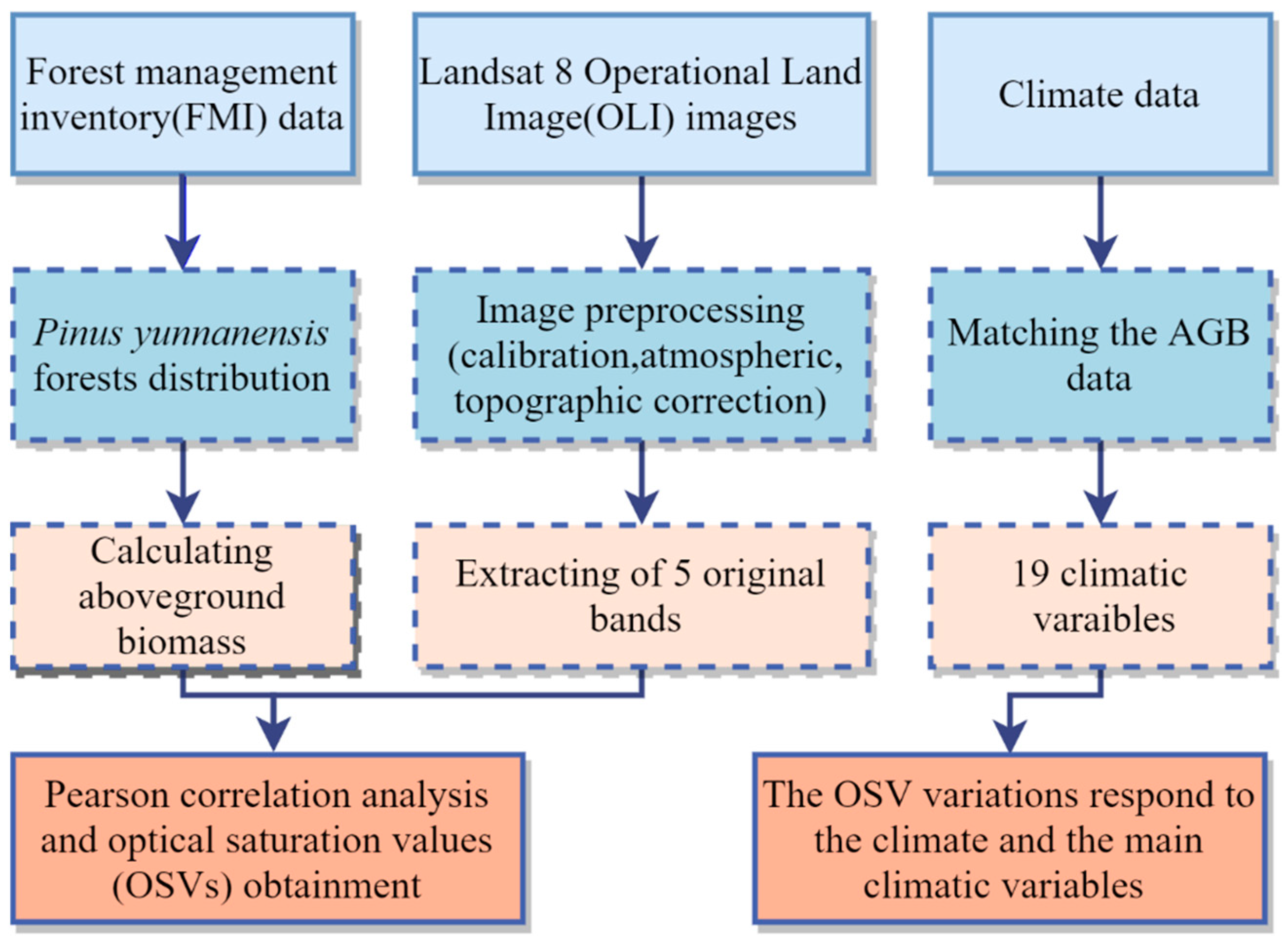
2. Materials and Methods
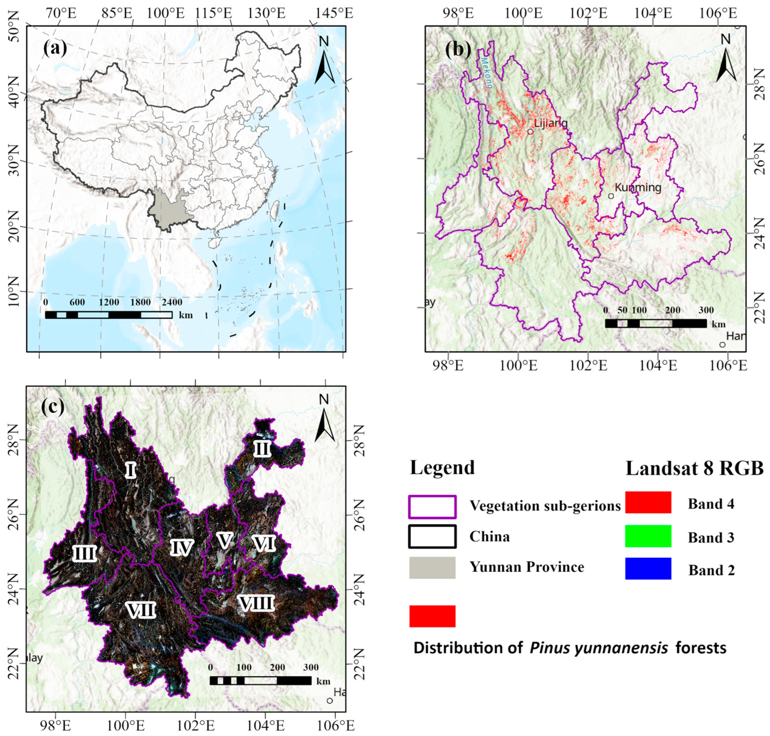
This study adhered to the methodological flowchart shown in Figure 1, with the following steps: (1) obtaining data on the distribution of Pinus yunnanensis forests from the Forest Management Inventory (FMI); (2) calculating the Pinus yunnanensis forests’ AGB across eight sub-regions classified by the Yunnan flora system; (3) collecting and processing Landsat 8 OLI imagery along with relevant climate data; (4) extracting the original spectral bands; (5) analyzing the correlation between forest AGB and the original bands; (6) applying the spherical model to calculate OSVs; (7) examining OSV variations in response to climatic factors; and (8) identifying the key climatic variables that influence OSV variations.

2.1. Study Area

Yunnan Province, located in southwestern China, extends between latitudes 21°8′ N and 29°15′ N and longitudes 97°31′ E to 106°11′ E, encompassing a total area of 394,000 km2 (Figure 2). It is in the region where the plateau and mountainous areas intersect, characterized by a complex and diverse topography including high mountains, canyons, hills, and plains. Its geographical location and complex terrain contribute to the high heterogeneity of climate, vegetation, and so on [26,32]. It exhibits a range of climatic types, including subtropical, temperate, and alpine climates. The altitude ranges from 76.4 m to 6740 m, while the precipitation varies between 500 mm and 2700 mm [18]. Meanwhile, the favorable climate in Yunnan provides optimal growth conditions for Pinus yunnanensis forests, enabling it to flourish in various ecological habitats, including subalpine forests, montane forests, and mixed evergreen–deciduous forests [33].

2.2. Vegetation Sub-Regions

The Yunnan flora system was utilized to divide the Yunnan province into 8 sub-regions using ArcGIS 10.8, which was produced by combining the relationships between the distribution and phylogenetics of seed plant genera in 1983 [34,35]. This segmentation facilitated the alignment of climate and Pinus yunnanensis forest AGB data, enabling the derivation and comparative analysis of OSVs across sub-regions to investigate their variations (Figure 2).

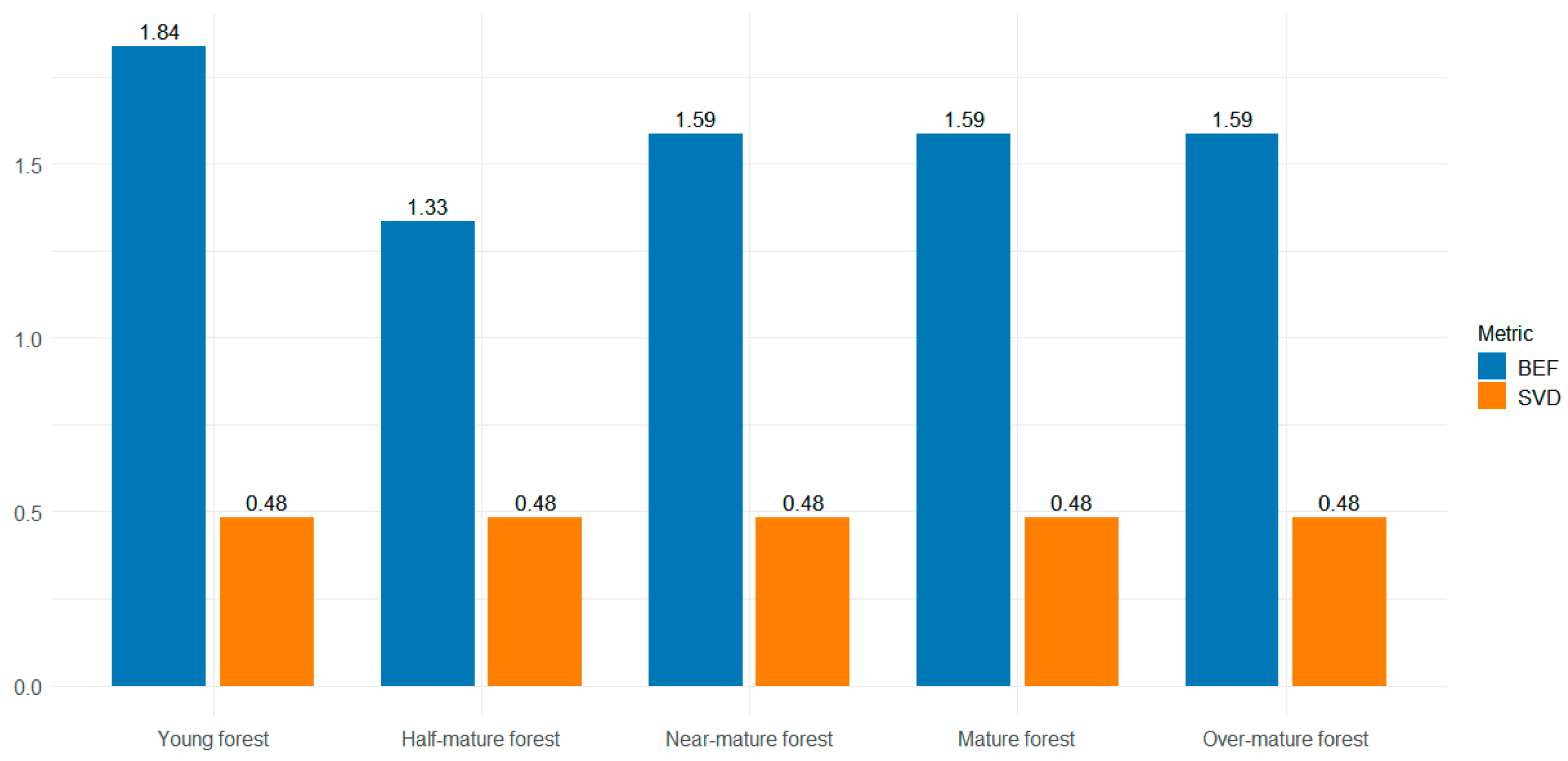
2.3. Forest Aboveground Biomass Data

The distribution of Pinus yunnanensis forests was obtained from the 2016 FMI data for Yunnan province. The AGB per unit area of Pinus yunnanensis forests was calculated using the biomass conversion method based on a total of 175,511 selected sub-compartments [36]. The biomass conversion parameters are shown in Figure 3. The formula used for AGB calculation is as follows:
B = V × S V D × B E F
where B refers to the AGB for the sub-compartment (t/ha), V indicates the volume of storage per unit area in the sub-compartment (m3/hm2), SVD stands for the basic wood density (t/m3), and BEF is the biomass conversion coefficient (dimensionless).
All sub-compartments of Pinus yunnanensis forests were selected to estimate OSVs, providing a thorough estimation of the forest’s spatial arrangement and AGB properties. The statistical metrics for each sub-region, including sample size, AGB range, mean AGB, and standard error, are detailed in Table 1. These values reveal significant variability in AGB across sub-regions. The standard error further underscores this heterogeneity, with sub-region I exhibiting marked variability (SE = 36.74 t/ha), while sub-region VI shows more consistency (SE = 18.33 t/ha). Such findings emphasize the need to account for regional differences in AGB and OSV estimations, given their sensitivity to local environmental dynamics.

2.4. Remote Sensing Data

The original bands of Landsat 8 OLI data were used to derive the OSVs, with a spatial resolution of 30 m. The 29 Landsat 8 OLI images from 2016 in Yunnan were acquired from a website (http://www.gscloud.cn/ (accessed on 1 April 2023)). A substantial portion of the images had a cloud cover of less than 6.00%. Subsequent image preprocessing included radiometric calibration, atmospheric correction using FLAASH, topographic correction, and geographic alignment to ensure reliable and consistent land cover and surface property analysis, utilizing ENVI 5.3 software [37,38]. Finally, simultaneous Landsat 8 OLI images with the forest AGB data from 2016 were mosaicked to produce a seamless image.

2.5. Climate Data

The climate data were obtained from the WorldClim database (http://www.worldclim.org/ (accessed on 1 April 2023)), with a spatial resolution of 1 km × 1 km, containing 19 bio-climatic variables (Table 2). The climate data were georeferenced in ENVI 5.3 to align with the Pinus yunnanensis distribution and sub-regional boundaries and resampled to 30 × 30 m resolution for compatibility with the Landsat 8 imagery.

2.6. Optical Saturation Values Obtainment

The study validated that the spherical model based on the semi-variance function provides highly accurate estimates for calculating OSVs both in Landsat TM [17] and Landsat 8 OLI imagery [18]. In this study, the spherical model was employed to estimate the OSVs using 5 bands, including Blue, Green, Red, NIR, and SWIR2, derived from Landsat 8 OLI imagery. The correlation between these bands and forest AGB was rigorously analyzed, with statistically significant correlations at the 0.01 level being selected. Subsequently, the OSVs were calculated across 8 sub-regions, allowing for a comprehensive analysis of OSV variations. The spherical model can be represented by the following equation:
y ( A G B ) = c 0 + c ( 3 A G B 2 B S A G B 3 2 B S 3 )   0 A G B B S c 0 + c   A G B > B S
where y(AGB) denotes the value of spectral reflectance; c0 denotes the reflectance when biomass is zero; c stands for the rate of change in reflectance; c0 + c signifies the maximum or minimum reflectance value when biomass reaches saturation; BS corresponds to the spectral OSV for the specific bands. By setting b 0 = c 0 ,   b 1 = 3 c / 2 B S ,   b 2 = c / 2 B S 3 ,   x = A G B , the AGB value can be derived through least squares regression. Through the application of least squares fitting to Equation (3), the parameters for Equations (4) and (5) are obtained, enabling the calculation of OSVs by incorporating parameters b 1 and b 2 from Equation (6).
y = b 0 + b 1 x + b 2 x 3
b 1 + b 2 = 3 c 2 O S V C 2 O S V 3
c = 2 3 O S V × b 1
OSV = b 1 3 b 2

2.7. Optical Saturation Values’ Variation Analyses

It was crucial to find the key variables affecting the OSV variations by clarifying the relationship between the OSVs and climatic variables. Canonical correlation analysis (CCA) is a statistical approach used to examine and quantify the linear relationships between two multivariate datasets [39,40]. Its advantages include revealing the correlations between multiple variables, dimensionality reduction, integration and interpretation of multiple datasets, and application in prediction and classification tasks [40,41]. Thus, CCA was applied to investigate the relationship between OSVs and climatic variables. The key factors influencing OSV variations were identified using the vegan package in R4.4.1 software as part of this study. Firstly, 19 climatic variables were standardized to ensure the variables were comparable across scales or units of measure, and we then eliminated the inequitable effects due to differences in the scales of variables [41]. Subsequently, standardized climatic variables and OSVs across 8 sub-regions underwent CCA, elucidating climate-responsive OSV variations and identifying key climatic determinants.

3. Results

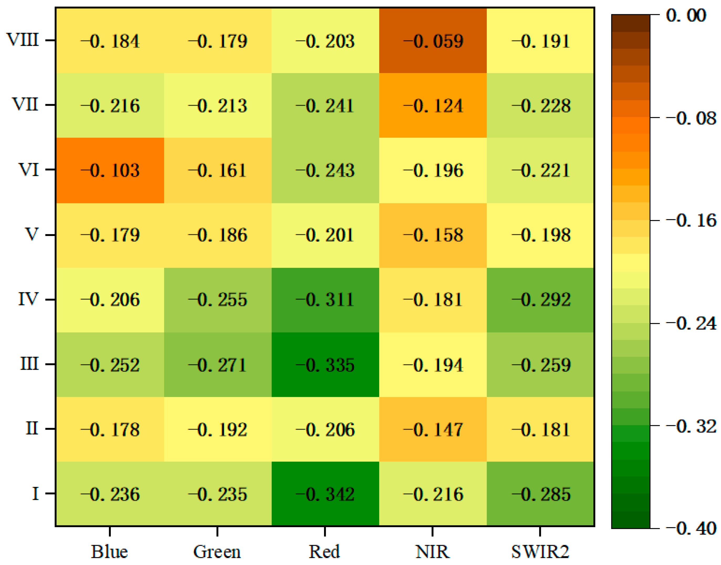
3.1. Relationship between Forest Aboveground Biomass and Original Spectral Bands

Pearson correlation analysis was utilized between the Pinus yunnanensis forest AGB and five original bands, and the results show that all the original bands were significant at the 0.01 level. As shown in Figure 4, all the original bands were negative with the Pinus yunnanensis forest AGB in each sub-region, and the Red band showed the best performance, with all the absolute values of correlation coefficients greater than 0.2.
A significance test was applied to assess the correlation between Pinus yunnanensis forest AGB and the five original spectral bands, aiming to determine if there were notable differences in how each band contributed to the estimation of OSVs for forest AGB estimation. As shown in Figure 5, most bands were not statistically significant, with only a few exceptions (* p < 0.05, ** p < 0.01). This indicates that no single band significantly outperformed the others in estimating OSVs. Consequently, all five bands were incorporated into the final analysis to compute OSVs for each sub-region. In a more detailed sense, it illustrates that the correlations across the bands were quite similar, with minor variations. While the NIR and Red bands displayed slightly stronger negative correlations, these differences were not pronounced enough to prioritize one band over the others. Therefore, utilizing all five bands provided a more comprehensive and robust approach to estimating saturation values across the different regions.

3.2. OSV Variation Analysis

The OSVs in each vegetation sub-region displayed significant differences when using the same band (Figure 6), though similar OSVs were observed across sub-regions with different bands. Additionally, the OSVs for Pinus yunnanensis forests in Yunnan Province ranged from 104.42 t/ha to 209.11 t/ha. The highest OSV (209.11 t/ha) was recorded in sub-region VII using the Red band, while the lowest OSV (104.42 t/ha) was observed in sub-region VIII using the Green band. Then, most sub-regions, such as I, II, III, and V, were approximately 180 t/ha. Overall, the variations of OSV in Pinus yunnanensis forests were extremely noteworthy in Yunnan, showing a trend of lowest in the southeast and highest in the southwest.

3.3. The OSV Variations Response to the Climate

As shown in Figure 7, the OSV variations in response to climate were clarified through CCA. The results reveal that the first axis accounted for 88.3% of the OSV variations, while the second axis explained 4.9%, making a total of 93.2% of the OSV variations attributed to climatic factors. Additionally, annual mean temperature (AMT) contributed the most to the CCA, highlighting temperature as a key factor influencing OSV variations. The mean temperature during the wettest quarter (MTQ) had the largest impact on the first axis, whereas annual average precipitation (ANP) made the highest contribution on the second axis. These findings demonstrate that both temperature and precipitation were the primary factors driving OSV variations. It was observed that the first axis favored temperature changes, while the second axis was more influenced by precipitation. Furthermore, the OSV variations were notable in groups A, B, C, and D, with the order of OSVs being D > C > B > A. In the four groups, the area of group A was warmer but the driest, the areas of group B were warmer and drier, the areas of group C were colder and wetter, and the areas of group D were the warmest and the wettest. Therefore, these indicators show that the OSV variations were mainly affected by the temperature and humidity.

4. Discussion

4.1. Original Bands

In this study, the original spectral bands exhibited a negative correlation with Pinus yunnanensis forests’ AGB, indicating a heightened capacity for light absorption and scattering in the forest vegetation [42]. This phenomenon resulted in greater light absorption within areas of dense forest cover, leading to correspondingly lower reflectance values [10,43]. Conversely, sub-regions characterized by lower biomass, such as bare ground or grasslands, exhibited higher reflectance [44,45]. This resulted in substantial differences in reflectance among various sub-regions within the Pinus yunnanensis forests. This observation is consistent with previous findings [46], yet it provides further validation of the pronounced light reflectance variability inherent in highly heterogeneous landscapes like Yunnan. Areas of higher biomass, especially those dominated by tree species such as Pinus yunnanensis, display significantly enhanced light absorption due to their dense canopy structure, offering valuable contributions to the use of spectral imaging technology in such complex ecosystems [47]. These results underscore the critical need to incorporate spatial variability into modeling efforts, thereby enhancing the precision of AGB estimation in other similarly heterogeneous forest systems [48].
The Red band exhibited the strongest performance among the original spectral bands, which can be attributed to the fact that chlorophyll in the leaves efficiently absorbs red light for photosynthesis. Chlorophyll has a pronounced absorption peak in the red waveband, enabling plants to capture red light with exceptional efficiency for energy conversion [49,50]. This absorption of red light by chlorophyll not only drives photosynthesis, but also stimulates increased plant growth and biomass accumulation [51,52]. The dense canopies and high tree density in Pinus yunnanensis forests, characterized by an extensive leaf area index due to their numerous clustered leaves, further enhance this effect [53]. Consequently, a higher concentration of chlorophyll is required in regions with substantial AGB, absorbing more red light to fuel photosynthesis and promote the synthesis of organic compounds. This contributes to the greater AGB observed in Pinus yunnanensis forests in Yunnan, which, in turn, further reduces overall reflectance [54,55]. These findings offer novel empirical support for understanding how spectral characteristics, particularly red light absorption, directly influence biomass accumulation in high-biomass vegetation types such as Pinus yunnanensis [56]. This relationship holds significant potential for refining remote sensing models that address biomass saturation challenges in highly heterogeneous regions [57]. Moreover, our study suggests that Red band reflectance could serve as a robust indicator for biomass estimation in other dense forest ecosystems, providing valuable insights for enhancing global biomass monitoring efforts [58].

4.2. OSV Variations

In this study, the largest OSV was 208.31 t/ha in sub-region VII, while the smallest OSV was 107.45 t/ha in sub-region VIII, with a mean OSV of 165.11 t/ha when assessing OSVs derived from the SWIR2 band. Comparatively, the OSVs across different vegetation types varied between 100 t/ha and 159 t/ha in Zhejiang Province, with pine forests reaching an OSV of 159 t/ha [17]. Notably, the average OSV for Pinus yunnanensis forests in Yunnan surpassed that of the pine forests in Zhejiang, likely due to the mountainous plateau topography, complex stand structure, and heightened forest heterogeneity in Yunnan [59]. High forest heterogeneity and complex stand structures were identified as the primary contributors to the saturation issue [6]. In comparison, an associated study examining OSVs for oak forests in Yunnan reported a range from 104 t/hm2 to 182 t/hm2 [18]. The disparity in OSV ranges between these studies can largely be attributed to the intrinsic structural and physiological differences between coniferous forests, like Pinus yunnanensis, and broadleaf forests, such as oak. Coniferous species typically have denser canopies with narrower leaves, affecting light absorption and scattering, whereas broadleaf species, with their larger and more complex leaves, generally exhibit higher photosynthetic activity and greater biomass accumulation, which may contribute to distinct OSV patterns across these forest types [60,61]. This study is among the first to offer a quantitative analysis of how complex topography and forest heterogeneity influence OSV variations in Pinus yunnanensis forests. It reveals that OSVs are notably higher in highly heterogeneous and mountainous regions, providing important theoretical support for understanding the role of topography in biomass saturation. These findings suggest that similar effects of heterogeneity may be observed in other diverse forest ecosystems, emphasizing the need for region-specific OSV models that account for topographical complexity [62].
Moreover, it was observed that OSVs varied across different sub-regions, regardless of which original bands were used, indicating that OSV variation patterns exist inherently to some extent. A discernible trend emerged for Pinus yunnanensis forests in Yunnan, with the highest OSV recorded in sub-region VII, higher OSVs in sub-regions I, II, III, IV, and V, and lower OSVs in sub-region VI, with the lowest value in sub-region VIII. This pattern suggests that OSVs for Pinus yunnanensis forests in Yunnan are the highest in the southwestern regions and lowest in the southeastern areas. The systematic analysis of OSV differences across these sub-regions not only highlights the spatial variability of OSVs, but also provides novel insights into how OSVs respond to geographical and climatic influences. This finding underscores the necessity of developing predictive models that accurately capture the spatial variability of OSVs, particularly in heterogeneous environments like Yunnan [63]. Additionally, these results highlight the potential for designing targeted biomass management strategies that consider specific OSV variation patterns across diverse forest ecosystems.

4.3. The Key Climatic Variables Affecting OSV Variations

The OSV variations were highly responsive to climatic conditions, with 93.2% of the variation explained by climatic variables through CCA. Among these, the AMT made the greatest contribution on the first axis, indicating that temperature is one of the primary factors influencing OSV variations. Temperature affects the absorption of red and other visible light by influencing plant photosynthesis, which in turn impacts plant growth and contributes to a more complex stand structure [64,65]. Additionally, the MTQ and ANP made the highest contributions on the first and second axes, respectively. MTQ is crucial as it reflects the temperature conditions during the peak growing season, when precipitation is at its highest, significantly impacting physiological processes such as photosynthesis and respiration. Favorable temperatures enhance plant growth, nutrient uptake, and photosynthetic activity, ultimately increasing species heterogeneity [66,67]. ANP plays a vital role in determining water availability within an ecosystem [68]. Sufficient precipitation is essential for plant growth, as it provides the necessary water for photosynthesis and other metabolic processes. Conversely, inadequate rainfall leads to water stress, limiting plant productivity [69], and resulting in a lower leaf area index (LAI) and higher band reflectance, which, in turn, lowers biomass saturation values. On the other hand, higher ANP creates optimal conditions for plant growth, allowing for increased LAI and reduced band reflectance [70], which leads to higher saturation values. This comprehensive examination of the climatic influence on OSV variability provides profound insights into the climatic determinants of forest AGB and addresses the issue of saturation. By systematically examining the influence of key variables such as temperature and precipitation, this study advances our understanding of how climatic factors shape the distribution and OSVs of forest AGB, providing a robust framework for future climate-based biomass models [71]. Moreover, our findings suggest that the interplay between temperature and precipitation could serve as a key predictor for monitoring forest AGB in similarly forested regions worldwide, contributing to more accurate AGB estimations under varying climatic conditions.
The results indicate that OSV variations were primarily influenced by temperature and humidity, as demonstrated through CCA. This can be explained by the pivotal role temperature plays in regulating various biochemical and physiological processes in plants [72]. Temperature affects the efficiency of photosynthesis, the rate of metabolic reactions, and the overall growth and development of vegetation [73]. Similarly, humidity is closely tied to water availability, which is crucial for plant growth and survival [74]. Adequate humidity levels provide sufficient moisture for root absorption, facilitating the transport of nutrients and energy, promoting leaf development, and reducing band reflectance [75]. In contrast, insufficient humidity can lead to water stress and diminished plant productivity [76]. The climate in Yunnan, characterized by significant variability in temperature and humidity due to geographical location, elevation, and seasonality [77], has shaped the region’s complex stand structure, diverse tree species composition, and heightened forest heterogeneity [9,78,79,80]. These findings enhance our understanding of the roles temperature and humidity play in shaping forest structural complexity and species diversity. This study’s comprehensive examination of the relationship between climate and OSV variability advances the discourse on climate-driven processes in forest ecosystems, offering valuable theoretical and practical insights for improving AGB estimation models in heterogeneous environments [81]. Furthermore, by highlighting the intricate interrelationships between temperature, humidity, and the saturation problem, this research underscores the importance of developing integrative models that incorporate multiple climatic variables across diverse ecological contexts [82]. Numerous studies have demonstrated that the saturation problem and its variations are primarily driven by complex forest stand structures, diverse species composition, and high forest heterogeneity [6,10,83]. Accordingly, the OSV variations in Pinus yunnanensis forests were interpreted in response to climate and key climatic variables, with temperature and humidity identified as the primary factors influencing OSV variability. This study not only corroborates prior research on the significance of forest structure and heterogeneity in OSV variation, but also offers a comprehensive analysis of the climatic factors that govern these variations. By identifying the critical role of temperature and humidity, this work deepens our understanding of the intricate interplay between climatic conditions and saturation problems in forest AGB estimation using optical imagery.

4.4. Limitations and Future Research

This study leveraged Landsat 8 OLI imagery to quantify OSVs in Pinus yunnanensis forests across Yunnan. While this sensor offers valuable spectral data and an extensive historical archive, it has inherent limitations that may introduce uncertainties in estimating OSVs. The 30 m spatial resolution, although effective for large-scale forest monitoring, may fall short in capturing the fine-scale heterogeneity of forests, particularly in regions like Yunnan, where diverse forest structures and complex terrain are prevalent. This limitation can result in mixed pixels, where signals represent multiple land cover types, thereby diminishing the accuracy of OSV estimates [84]. Meanwhile, its lower spectral resolution compared to high-resolution sensors like WorldView-3 or hyperspectral platforms may result in the inadequate detection of subtle vegetation variations, potentially causing biomass overestimation or underestimation, especially in high-biomass areas susceptible to saturation effects [85]. Then, this study highlighted the limitations of using year-round data, which, while comprehensive, do not differentiate between the growing and non-growing seasons. Since vegetation productivity and spectral reflectance tend to peak during the growing season, this may impact OSV estimates [86]. We should explore seasonal data separation to better account for variations in vegetation dynamics across different times of the year in future research. Furthermore, other research found that the OSV was 192 t/ha using the Landsat 8 OLI, 247 t/ha using the Worldview-3, and 204 t/ha using Sentinel-2 MSI images [87], indicating that various remote sensing data had different saturation values [10]. Therefore, it is essential to investigate alternative remote sensing sources, including Sentinel-2, SPOT, MODIS, and QuickBird, for use in estimating forest AGB and OSV variations, particularly in areas of high forest heterogeneity.
Despite these sensor limitations, this study identified key climatic variables influencing OSV variations, with AMT emerging as the most significant factor using CCA. However, whether the inclusion of these climatic variables can enhance AGB estimation accuracy using Landsat 8 OLI remains an open question for future research. The observed OSV variations were also responsive to temperature and humidity, underscoring the need for further exploration into how OSV dynamics interact with climatic and environmental factors across diverse tree species and regions. It is crucial to explore the responses of the OSV variations using optical images of other tree species to climate and other environmental factors correspondingly.

5. Conclusions

This study analyzes how climatic factors influence OSV variations and identifies the key variables affecting these variations in Pinus yunnanensis forests using Landsat 8 OLI imagery. OSVs were analyzed across eight sub-regions of Yunnan Province, China, and CCA was used to determine the main climatic drivers. The results show that the Red band of Landsat 8 OLI had the strongest performance, with OSVs ranging from 104.42 t/ha to 209.11 t/ha, peaking in the southwest and being the lowest in the southeast. The CCA revealed that 93.2% of the OSV variation could be explained by climate, with temperature and humidity emerging as the most significant factors. The AMT was the highest-contributing variable of 19 climate variables, and the MTQ and ANP made the highest contributions in the first and second axes, respectively. Ultimately, it was found that the hydrothermal conditions were the main factors affecting the OSV variations at the general level, and the OSVs were larger in the warmer and wetter sub-regions.

Author Contributions

Y.W. participated in the collection of the data, conducted the data analysis, and wrote the draft of the paper; B.G., X.Z., H.L. (Hongbin Luo), Z.Y., H.L. (Huipeng Li) and K.S. helped with the data analysis, and constructed part of the graphs; L.W. and W.X. gave some suggestions and guidance; G.O. supervised and coordinated the research project, designed the experiment and revised the paper. All authors have read and agreed to the published version of the manuscript.

Funding

This research was jointly supported by the Ten Thousand Talent Plans for Young Top-notch Talents of Yunnan Province (YNWR-QNBJ-2018-184), the Scientific Research Fund Project of Yunnan Provincial Education Department (2023Y0732), and the Education Talent of Xingdian Talent Support Program of Yunnan Province, China.

Data Availability Statement

The original contributions presented in this study are included in the article, and further inquiries can be directed to the corresponding authors.

Acknowledgments

We would like to acknowledge all the people who have contributed to this paper.

Conflicts of Interest

The authors declare no conflicts of interest.

References

  1. Schimel, D.S. Terrestrial ecosystems and the carbon cycle. Glob. Chang. Biol. 1995, 1, 77–91. [Google Scholar] [CrossRef]
  2. Pearce, D.W. The economic value of forest ecosystems. Ecosyst. Health 2001, 7, 284–296. [Google Scholar] [CrossRef]
  3. Mitchard, E.T. The tropical forest carbon cycle and climate change. Nature 2018, 559, 527–534. [Google Scholar] [CrossRef] [PubMed]
  4. Keith, H.; Mackey, B.G.; Lindenmayer, D.B. Re-evaluation of forest biomass carbon stocks and lessons from the world’s most carbon-dense forests. Proc. Natl. Acad. Sci. USA 2009, 106, 11635–11640. [Google Scholar] [CrossRef] [PubMed]
  5. Sileshi, G.W. A critical review of forest biomass estimation models, common mistakes and corrective measures. For. Ecol. Manag. 2014, 329, 237–254. [Google Scholar] [CrossRef]
  6. Lu, D.; Chen, Q.; Wang, G.; Liu, L.; Li, G.; Moran, E. A survey of remote sensing-based aboveground biomass estimation methods in forest ecosystems. Int. J. Digital Earth 2016, 9, 63–105. [Google Scholar] [CrossRef]
  7. Tian, X.; Su, Z.; Chen, E.; Li, Z.; van der Tol, C.; Guo, J.; He, Q. Reprint of: Estimation of forest above-ground biomass using multi-parameter remote sensing data over a cold and arid area. Int. J. Appl. Earth Obs. Geoinf. 2012, 17, 102–110. [Google Scholar] [CrossRef]
  8. Silveira, E.M.; Silva, S.H.G.; Acerbi-Junior, F.W.; Carvalho, M.C.; Carvalho, L.M.T.; Scolforo, J.R.S.; Wulder, M.A. Object-based random forest modelling of aboveground forest biomass outperforms a pixel-based approach in a heterogeneous and mountain tropical environment. Int. J. Appl. Earth Obs. Geoinf. 2019, 78, 175–188. [Google Scholar] [CrossRef]
  9. Ou, G.; Li, C.; Lv, Y.; Wei, A.; Xiong, H.; Xu, H.; Wang, G. Improving aboveground biomass estimation of Pinus densata forests in Yunnan using Landsat 8 imagery by incorporating age dummy variable and method comparison. Remote Sens. 2019, 11, 738. [Google Scholar] [CrossRef]
  10. Mutanga, O.; Masenyama, A.; Sibanda, M. Spectral saturation in the remote sensing of high-density vegetation traits: A systematic review of progress, challenges, and prospects. ISPRS J. Photogramm. Remote Sens. 2023, 198, 297–309. [Google Scholar] [CrossRef]
  11. Allen, W.A.; Richardson, A.J. Interaction of light with a plant canopy. JOSA 1968, 58, 1023–1028. [Google Scholar] [CrossRef]
  12. Di Bella, C.; Paruelo, J.; Becerra, J.; Bacour, C.; Baret, F. Effect of senescent leaves on NDVI-based estimates of APAR: Experimental and modelling evidences. Int. J. Remote Sens. 2004, 25, 5415–5427. [Google Scholar] [CrossRef]
  13. Tucker, C.J. Red and photographic infrared linear combinations for monitoring vegetation. Remote Sens. Environ. 1979, 8, 127–150. [Google Scholar] [CrossRef]
  14. Steininger, M. Satellite estimation of tropical secondary forest above-ground biomass: Data from Brazil and Bolivia. Int. J. Remote Sens. 2000, 21, 1139–1157. [Google Scholar] [CrossRef]
  15. Mutanga, O.; Skidmore, A.K. Hyperspectral band depth analysis for a better estimation of grass biomass (Cenchrus ciliaris) measured under controlled laboratory conditions. Int. J. Appl. Earth Obs. Geoinf. 2004, 5, 87–96. [Google Scholar] [CrossRef]
  16. Zhu, X.; Liu, D. Improving forest aboveground biomass estimation using seasonal Landsat NDVI time-series. ISPRS J. Photogramm. Remote Sens. 2015, 102, 222–231. [Google Scholar] [CrossRef]
  17. Zhao, P.; Lu, D.; Wang, G.; Wu, C.; Huang, Y.; Yu, S. Examining spectral reflectance saturation in Landsat imagery and corresponding solutions to improve forest aboveground biomass estimation. Remote Sens. 2016, 8, 469. [Google Scholar] [CrossRef]
  18. Wu, Y.; Ou, G.; Huang, T.; Zhang, X.; Liu, C.; Liu, Z.; Yu, Z.; Luo, H.; Lu, C.; Shi, K. Climate Interprets Saturation Value Variations Better Than Soil and Topography in Estimating Oak Forest Aboveground Biomass Using Landsat 8 OLI Imagery. Remote Sens. 2024, 16, 1338. [Google Scholar] [CrossRef]
  19. Sturrock, R.; Frankel, S.; Brown, A.; Hennon, P.; Kliejunas, J.; Lewis, K.; Worrall, J.; Woods, A. Climate change and forest diseases. Plant Pathol. 2011, 60, 133–149. [Google Scholar] [CrossRef]
  20. Xia, Y.; Hao, H.; Zanardo, G.; Deeks, A. Long term vibration monitoring of an RC slab: Temperature and humidity effect. Eng. Struct. 2006, 28, 441–452. [Google Scholar] [CrossRef]
  21. Ainsworth, E.A.; Yendrek, C.R.; Sitch, S.; Collins, W.J.; Emberson, L.D. The effects of tropospheric ozone on net primary productivity and implications for climate change. Annu. Rev. Plant Biol. 2012, 63, 637–661. [Google Scholar] [CrossRef] [PubMed]
  22. Gray, S.B.; Brady, S.M. Plant developmental responses to climate change. Dev. Biol. 2016, 419, 64–77. [Google Scholar] [CrossRef] [PubMed]
  23. Ahanger, M.A.; Tomar, N.S.; Tittal, M.; Argal, S.; Agarwal, R. Plant growth under water/salt stress: ROS production; antioxidants and significance of added potassium under such conditions. Physiol. Mol. Biol. Plants 2017, 23, 731–744. [Google Scholar] [CrossRef] [PubMed]
  24. Chelli, S.; Bricca, A.; Tsakalos, J.L.; Andreetta, A.; Bonari, G.; Campetella, G.; Carnicelli, S.; Cervellini, M.; Puletti, N.; Wellstein, C. Multiple drivers of functional diversity in temperate forest understories: Climate, soil, and forest structure effects. Sci. Total Environ. 2024, 916, 170258. [Google Scholar] [CrossRef] [PubMed]
  25. Yang, Y.; Tian, K.; Hao, J.; Pei, S.; Yang, Y. Biodiversity and biodiversity conservation in Yunnan, China. Biodivers. Conserv. 2004, 13, 813–826. [Google Scholar] [CrossRef]
  26. Li, X.; Walker, D. The plant geography of Yunnan Province, southwest China. J. Biogeogr. 1986, 14, 367–397. [Google Scholar]
  27. Shen, J.; Li, Z.; Gao, C.; Li, S.; Huang, X.; Lang, X.; Su, J. Radial growth response of Pinus yunnanensis to rising temperature and drought stress on the Yunnan Plateau, southwestern China. For. Ecol. Manage. 2020, 474, 118357. [Google Scholar] [CrossRef]
  28. Wu, Y.; Ou, G.; Lu, T.; Huang, T.; Zhang, X.; Liu, Z.; Yu, Z.; Guo, B.; Wang, E.; Feng, Z. Improving Aboveground Biomass Estimation in Lowland Tropical Forests across Aspect and Age Stratification: A Case Study in Xishuangbanna. Remote Sens. 2024, 16, 1276. [Google Scholar] [CrossRef]
  29. Felipe-Lucia, M.R.; Soliveres, S.; Penone, C.; Manning, P.; van der Plas, F.; Boch, S.; Prati, D.; Ammer, C.; Schall, P.; Gossner, M.M. Multiple forest attributes underpin the supply of multiple ecosystem services. Nature Commun. 2018, 9, 4839. [Google Scholar] [CrossRef]
  30. Swanson, M.E.; Franklin, J.F.; Beschta, R.L.; Crisafulli, C.M.; DellaSala, D.A.; Hutto, R.L.; Lindenmayer, D.B.; Swanson, F.J. The forgotten stage of forest succession: Early-successional ecosystems on forest sites. Front. Ecol. Environ. 2011, 9, 117–125. [Google Scholar] [CrossRef]
  31. Duivenvoorden, J.E. Tree species composition and rain forest-environment relationships in the middle Caquetá area, Colombia, NW Amazonia. Vegetation 1995, 120, 91–113. [Google Scholar] [CrossRef]
  32. Peng, J.; Yang, Y.; Liu, Y.; Du, Y.; Meersmans, J.; Qiu, S. Linking ecosystem services and circuit theory to identify ecological security patterns. Sci. Total Environ. 2018, 644, 781–790. [Google Scholar] [CrossRef]
  33. Zhang, Y. Water and Carbon Balances of Deciduous and Evergreen Broadleaf Trees from a Subtropical Cloud Forest in Southwest China. Ph.D. Thesis, University of Miami, Coral Gables, FL, USA, 2012. [Google Scholar]
  34. Li, R.; Kraft, N.J.; Yang, J.; Wang, Y. A phylogenetically informed delineation of floristic regions within a biodiversity hotspot in Yunnan, China. Sci. Rep. 2015, 5, 9396. [Google Scholar] [CrossRef] [PubMed]
  35. Fang, P.; Ou, G.; Li, R.; Wang, L.; Xu, W.; Dai, Q.; Huang, X. Regionalized classification of stand tree species in mountainous forests by fusing advanced classifiers and ecological niche model. GISci. Remote Sens. 2023, 60, 2211881. [Google Scholar] [CrossRef]
  36. Xu, H.; Zhang, Z.; Ou, G.; Shi, H. A Study on Estimation and Distribution for Forest Biomass and Carbon Storage in Yunnan Province; Yunnan Science and Technology Press: Kunming, China, 2019. [Google Scholar]
  37. Kaufman, Y.J.; Tanre, D. Strategy for direct and indirect methods for correcting the aerosol effect on remote sensing: From AVHRR to EOS-MODIS. Remote Sens. Environ. 1996, 55, 65–79. [Google Scholar] [CrossRef]
  38. Young, N.E.; Anderson, R.S.; Chignell, S.M.; Vorster, A.G.; Lawrence, R.; Evangelista, P.H. A survival guide to Landsat preprocessing. Ecology 2017, 98, 920–932. [Google Scholar] [CrossRef]
  39. Thompson, B. Canonical correlation analysis. In Handbook of Applied Multivariate Statistics and Mathematical Modeling; Elsevier: Amsterdam, The Netherlands, 2000. [Google Scholar]
  40. Andrew, G.; Arora, R.; Bilmes, J.; Livescu, K. Deep canonical correlation analysis. In Proceedings of the International Conference on Machine Learning, Atlanta, GA, USA, 16–21 June 2013; pp. 1247–1255. [Google Scholar]
  41. Hardoon, D.R.; Szedmak, S.; Shawe-Taylor, J. Canonical correlation analysis: An overview with application to learning methods. Neural Comput. 2004, 16, 2639–2664. [Google Scholar] [CrossRef]
  42. Ollinger, S.V. Sources of variability in canopy reflectance and the convergent properties of plants. New Phytol. 2011, 189, 375–394. [Google Scholar] [CrossRef]
  43. Gao, X.; Huete, A.R.; Ni, W.; Miura, T. Optical–biophysical relationships of vegetation spectra without background contamination. Remote Sens. Environ. 2000, 74, 609–620. [Google Scholar] [CrossRef]
  44. Jin, Y.; Yang, X.; Qiu, J.; Li, J.; Gao, T.; Wu, Q.; Zhao, F.; Ma, H.; Yu, H.; Xu, B. Remote sensing-based biomass estimation and its spatio-temporal variations in temperate grassland, Northern China. Remote Sens. 2014, 6, 1496–1513. [Google Scholar] [CrossRef]
  45. Hütt, C.; Bolten, A.; Hüging, H.; Bareth, G. Uav lidar metrics for monitoring crop height, biomass and nitrogen uptake: A case study on a winter wheat field trial. PFG–J. Photogramm. Remote Sens. Geoinf. Sci. 2023, 91, 65–76. [Google Scholar] [CrossRef]
  46. Chave, J.; Réjou-Méchain, M.; Búrquez, A.; Chidumayo, E.; Colgan, M.S.; Delitti, W.B.; Duque, A.; Eid, T.; Fearnside, P.M.; Goodman, R.C. Improved allometric models to estimate the aboveground biomass of tropical trees. Global Chang. Biol. 2014, 20, 3177–3190. [Google Scholar] [CrossRef] [PubMed]
  47. Schimel, D.; Pavlick, R.; Fisher, J.B.; Asner, G.P.; Saatchi, S.; Townsend, P.; Miller, C.; Frankenberg, C.; Hibbard, K.; Cox, P. Observing terrestrial ecosystems and the carbon cycle from space. Glob. Chang. Biol. 2015, 21, 1762–1776. [Google Scholar] [CrossRef] [PubMed]
  48. Gitelson, A.A.; Peng, Y.; Arkebauer, T.J.; Schepers, J. Relationships between gross primary production, green LAI, and canopy chlorophyll content in maize: Implications for remote sensing of primary production. Remote Sens. Environ. 2014, 144, 65–72. [Google Scholar] [CrossRef]
  49. Huete, A.; Liu, H.; Batchily, K.; Van Leeuwen, W. A comparison of vegetation indices over a global set of TM images for EOS-MODIS. Remote Sens. Environ. 1997, 59, 440–451. [Google Scholar] [CrossRef]
  50. Terashima, I.; Fujita, T.; Inoue, T.; Chow, W.S.; Oguchi, R. Green light drives leaf photosynthesis more efficiently than red light in strong white light: Revisiting the enigmatic question of why leaves are green. Plant Cell Physiol. 2009, 50, 684–697. [Google Scholar] [CrossRef]
  51. Zhu, L.; Bloomfield, K.J.; Hocart, C.H.; Egerton, J.J.; O’Sullivan, O.S.; Penillard, A.; Weerasinghe, L.K.; Atkin, O.K. Plasticity of photosynthetic heat tolerance in plants adapted to thermally contrasting biomes. Plant Cell Environ. 2018, 41, 1251–1262. [Google Scholar] [CrossRef]
  52. Moriwaki, T.; Falcioni, R.; Tanaka, F.A.O.; Cardoso, K.A.K.; Souza, L.; Benedito, E.; Nanni, M.R.; Bonato, C.M.; Antunes, W.C. Nitrogen-improved photosynthesis quantum yield is driven by increased thylakoid density, enhancing green light absorption. Plant Sci. 2019, 278, 1–11. [Google Scholar] [CrossRef]
  53. Lin, Q.; Huang, H.; Chen, L.; Wang, J.; Huang, K.; Liu, Y. Using the 3D model RAPID to invert the shoot dieback ratio of vertically heterogeneous Yunnan pine forests to detect beetle damage. Remote Sens. Environ. 2021, 260, 112475. [Google Scholar] [CrossRef]
  54. Chen, L.; Wang, Y.; Ren, C.; Zhang, B.; Wang, Z. Optimal combination of predictors and algorithms for forest above-ground biomass mapping from Sentinel and SRTM data. Remote Sens. 2019, 11, 414. [Google Scholar] [CrossRef]
  55. Tu, J.; Li, Z.; Xu, Y.; Sun, J.; Zhao, X.; Huang, Z. Sapling root ecological stoichiometric characteristics of dominant species in three forests in Yunnan, China, and their relationship with soil physicochemical factors. Appl. Veg. Sci. 2022, 33, e13166. [Google Scholar] [CrossRef]
  56. Ali, I.; Greifeneder, F.; Stamenkovic, J.; Neumann, M.; Notarnicola, C. Review of machine learning approaches for biomass and soil moisture retrievals from remote sensing data. Remote Sens. 2015, 7, 16398–16421. [Google Scholar] [CrossRef]
  57. Houghton, R.; Lawrence, K.; Hackler, J.; Brown, S. The spatial distribution of forest biomass in the Brazilian Amazon: A comparison of estimates. Glob. Chang. Biol. 2001, 7, 731–746. [Google Scholar] [CrossRef]
  58. Kobayashi, H.; Dye, D.G. Atmospheric conditions for monitoring the long-term vegetation dynamics in the Amazon using normalized difference vegetation index. Remote Sens. Environ. 2005, 97, 519–525. [Google Scholar] [CrossRef]
  59. Liu, S.; An, N.; Yang, J.; Dong, S.; Wang, C.; Yin, Y. Prediction of soil organic matter variability associated with different land use types in mountainous landscape in southwestern Yunnan province, China. Catena 2015, 133, 137–144. [Google Scholar] [CrossRef]
  60. Asner, G.P.; Scurlock, J.M.; Hicke, J.A. Global synthesis of leaf area index observations: Implications for ecological and remote sensing studies. Global Ecol. Biogeogr. 2003, 12, 191–205. [Google Scholar] [CrossRef]
  61. Niinemets, Ü. Responses of forest trees to single and multiple environmental stresses from seedlings to mature plants: Past stress history, stress interactions, tolerance and acclimation. For. Ecol. Manag. 2010, 260, 1623–1639. [Google Scholar] [CrossRef]
  62. Saatchi, S.S.; Harris, N.L.; Brown, S.; Lefsky, M.; Mitchard, E.T.; Salas, W.; Zutta, B.R.; Buermann, W.; Lewis, S.L.; Hagen, S. Benchmark map of forest carbon stocks in tropical regions across three continents. Proc. Natl. Acad. Sci. USA 2011, 108, 9899–9904. [Google Scholar] [CrossRef]
  63. Harris, N.L.; Brown, S.; Hagen, S.C.; Saatchi, S.S.; Petrova, S.; Salas, W.; Hansen, M.C.; Potapov, P.V.; Lotsch, A. Baseline map of carbon emissions from deforestation in tropical regions. Science 2012, 336, 1573–1576. [Google Scholar] [CrossRef]
  64. Ahmed, H.A.; Tong, Y.-X.; Yang, Q.-C. Optimal control of environmental conditions affecting lettuce plant growth in a controlled environment with artificial lighting: A review. S. Afr. J. Bot. 2020, 130, 75–89. [Google Scholar] [CrossRef]
  65. Lichtenthaler, H.K.; Rinderle, U. The role of chlorophyll fluorescence in the detection of stress conditions in plants. Crit Rev. Anal. Chem. 1988, 19, S29–S85. [Google Scholar] [CrossRef]
  66. Usoltsev, V.A.; Zukow, W.; Osmirko, A.A.; Tsepordey, I.S.; Chasovskikh, V.P. Additive biomass models for Quercus spp. single-trees sensitive to temperature and precipitation in Eurasia. Ecol. Questi. 2019, 30, 29–40. [Google Scholar] [CrossRef]
  67. Hatfield, J.L.; Prueger, J.H. Temperature extremes: Effect on plant growth and development. Weather Clim. Extrem. 2015, 10, 4–10. [Google Scholar] [CrossRef]
  68. Margalef, O.; Sardans, J.; Fernández-Martínez, M.; Molowny-Horas, R.; Janssens, I.; Ciais, P.; Goll, D.; Richter, A.; Obersteiner, M.; Asensio, D. Global patterns of phosphatase activity in natural soils. Sci. Rep. 2017, 7, 1337. [Google Scholar] [CrossRef] [PubMed]
  69. Ali, M.; Talukder, M. Increasing water productivity in crop production—A synthesis. Agric. Water Manag. 2008, 95, 1201–1213. [Google Scholar] [CrossRef]
  70. Han, T.; Ren, H.; Wang, J.; Lu, H.; Song, G.; Chazdon, R.L. Variations of leaf eco-physiological traits in relation to environmental factors during forest succession. Ecol. Indic. 2020, 117, 106511. [Google Scholar] [CrossRef]
  71. Baccini, A.; Goetz, S.; Walker, W.; Laporte, N.; Sun, M.; Sulla-Menashe, D.; Hackler, J.; Beck, P.; Dubayah, R.; Friedl, M. Estimated carbon dioxide emissions from tropical deforestation improved by carbon-density maps. Nat. Clim. Chang. 2012, 2, 182–185. [Google Scholar] [CrossRef]
  72. Cohen, I.; Zandalinas, S.I.; Huck, C.; Fritschi, F.B.; Mittler, R. Meta-analysis of drought and heat stress combination impact on crop yield and yield components. Physiol. Plant. 2021, 171, 66–76. [Google Scholar] [CrossRef]
  73. Tripathy, B.C.; Brown, C.S.; Levine, H.G.; Krikorian, A.D. Growth and photosynthetic responses of wheat plants grown in space. Plant Physiol. 1996, 110, 801–806. [Google Scholar] [CrossRef]
  74. Passioura, J.B. Drought and drought tolerance. Plant Growth Regul. 1996, 20, 79–83. [Google Scholar] [CrossRef]
  75. Grossiord, C.; Buckley, T.N.; Cernusak, L.A.; Novick, K.A.; Poulter, B.; Siegwolf, R.T.; Sperry, J.S.; McDowell, N.G. Plant responses to rising vapor pressure deficit. New Phytol. 2020, 226, 1550–1566. [Google Scholar] [CrossRef] [PubMed]
  76. Blum, A. Effective use of water (EUW) and not water-use efficiency (WUE) is the target of crop yield improvement under drought stress. Field Crops Res. 2009, 112, 119–123. [Google Scholar] [CrossRef]
  77. Rangwala, I.; Miller, J.R. Climate change in mountains: A review of elevation-dependent warming and its possible causes. Clim. Chang. 2012, 114, 527–547. [Google Scholar] [CrossRef]
  78. Jin, Y.; Liu, C.; Qian, S.S.; Luo, Y.; Zhou, R.; Tang, J.; Bao, W. Large-scale patterns of understory biomass and its allocation across China’s forests. Sci. Total Environ. 2022, 804, 150169. [Google Scholar] [CrossRef] [PubMed]
  79. Zheng, Z.; Feng, Z.; Cao, M.; Li, Z.; Zhang, J. Forest Structure and Biomass of a Tropical Seasonal Rain Forest in Xishuangbanna, Southwest China. Biotropica J. Biol. Conserv. 2006, 38, 318–327. [Google Scholar]
  80. Meng, L.-Z.; Martin, K.; Weigel, A.; Liu, J.-X. Impact of rubber plantation on carabid beetle communities and species distribution in a changing tropical landscape (southern Yunnan, China). J. Insect Conserv. 2012, 16, 423–432. [Google Scholar] [CrossRef]
  81. Lawrence, D.; Vandecar, K. Effects of tropical deforestation on climate and agriculture. Nat. Clim. Chang. 2015, 5, 27–36. [Google Scholar] [CrossRef]
  82. Nemani, R.R.; Keeling, C.D.; Hashimoto, H.; Jolly, W.M.; Piper, S.C.; Tucker, C.J.; Myneni, R.B.; Running, S.W. Climate-driven increases in global terrestrial net primary production from 1982 to 1999. Science 2003, 300, 1560–1563. [Google Scholar] [CrossRef]
  83. Gleason, C.J.; Im, J. A review of remote sensing of forest biomass and biofuel: Options for small-area applications. GISci. Remote Sens. 2011, 48, 141–170. [Google Scholar] [CrossRef]
  84. Huang, T.; Ou, G.; Wu, Y.; Zhang, X.; Liu, Z.; Xu, H.; Xu, X.; Wang, Z.; Xu, C. Estimating the Aboveground Biomass of Various Forest Types with High Heterogeneity at the Provincial Scale Based on Multi-Source Data. Remote Sens. 2023, 15, 3550. [Google Scholar] [CrossRef]
  85. Choudhury, M.A.M.; Marcheggiani, E.; Galli, A.; Modica, G.; Somers, B. Mapping the urban atmospheric carbon stock by lidar and worldview-3 data. Forests 2021, 12, 692. [Google Scholar] [CrossRef]
  86. Hardisky, M.A.; Daiber, F.C.; Roman, C.T.; Klemas, V. Remote sensing of biomass and annual net aerial primary productivity of a salt marsh. Remote Sens. Environ. 1984, 16, 91–106. [Google Scholar] [CrossRef]
  87. Jha, N.; Tripathi, N.K.; Barbier, N.; Virdis, S.G.; Chanthorn, W.; Viennois, G.; Brockelman, W.Y.; Nathalang, A.; Tongsima, S.; Sasaki, N. The real potential of current passive satellite data to map aboveground biomass in tropical forests. Remote Sens. Ecol. Conserv. 2021, 7, 504–520. [Google Scholar] [CrossRef]
Figure 1. Methodological flowchart for estimating and analyzing OSV distribution patterns and variations.
Land 13 01534 g001
Figure 2. Overview of vegetation sub-regions and Pinus yunnanensis forests distribution: (a) illustrates the geographic location of Yunnan Province within China; (b) presents the spatial distribution of Pinus yunnanensis forests within Yunnan; and (c) shows Landsat 8 OLI imagery and eight sub-regions (I to VIII) within Yunnan.
Land 13 01534 g002
Figure 3. The parameters using the biomass conversion factor method.
Land 13 01534 g003
Figure 4. Relationship between Pinus yunnanensis forest AGB and the 5 original bands, with all original bands showing significance at the 0.01 level across the 8 sub-regions.
Land 13 01534 g004
Figure 5. The significance test of the correlations between five original bands and Pinus yunnanensis forest AGB. Double asterisks (**) indicate significance at the 0.01 level (p < 0.01), while a single asterisk (*) denotes significance at the 0.05 level (p < 0.05).
Land 13 01534 g005
Figure 6. The OSVs derived from the 5 original bands in each vegetation sub-region; (ae) correspond to the values obtained from the Blue, Green, Red, NIR, and SWIR2 bands.
Land 13 01534 g006
Figure 7. Analysis of the impact of climate variables on OSV variations using CCA: (a) relationship between OSVs and climate variables; (b) rates of contribution of climate variables to OSV variations.
Land 13 01534 g007
Table 1. The statistical parameters of each sub-region for Pinus yunnanensis forest AGB.
Sub-RegionsnAGB Range (t/ha)Mean (t/ha)SE (t/ha)
I45,4092.35–332.7056.7736.74
II24781.64–373.0939.6818.49
III11,0853.05–433.9364.3535.45
IV39,5692.58–485.4142.4723.59
V11,8261.01–485.4143.0326.52
VI16,5473.56–264.2037.1318.33
VII23,7662.84–339.9865.9128.35
VIII21,9391.89–220.4840.5622.10
Table 2. The overview of climate variables.
VariablesDescriptionsVariablesDescriptions
AMTAnnual mean temperature (°C)PRDPrecipitation in the driest quarter (mm)
MDRTemperature diurnal range (°C)PRSPrecipitation seasonality (mm)
ISOIsothermality (%)PWQPrecipitation in the warmest quarter (mm)
MCQMean temperature in the coldest quarter (°C)PCQPrecipitation in the coldest quarter (mm)
MTWTemperature in the warmest month (°C)PWMPrecipitation in the wettest month (mm)
MTCTemperature in the coldest month (°C)PDMPrecipitation in the driest month (mm)
TARTemperature annual range (°C)TESTemperature seasonality (°C)
MWQMean temperature in the warmest quarter (°C)PRWPrecipitation in the wettest quarter (mm)
MTDMean temperature in the driest quarter (°C)ANPMean of annual precipitation (mm)
MTQMean temperature in the wettest quarter (°C)
Disclaimer/Publisher’s Note: The statements, opinions and data contained in all publications are solely those of the individual author(s) and contributor(s) and not of MDPI and/or the editor(s). MDPI and/or the editor(s) disclaim responsibility for any injury to people or property resulting from any ideas, methods, instructions or products referred to in the content.

