Development of a Differential Spatial Economic Modeling Method for Improved Land Use and Multimodal Transportation Planning

Abstract

Regional planning agencies increasingly rely on Spatial Economic Models (SEMs) to evaluate the impact of various policies. However, traditional SEMs often employ homogeneous technical coefficients (TCs) to represent technology patterns used by activities located in very different areas of a region, leading to misrepresentations of production and consumption behaviors, and consequently, inaccurate modeling results. To this end, we propose a Differential Spatial Economic Modeling (DSEM) framework that incorporates region-specific TCs for activities within Independent Planning Units (IPUs), such as provinces or cities, each characterized by unique economic, demographic, and technological features. The DSEM framework comprises three core components: (1) a regional economy model that forecasts activity totals for each IPU using economic and demographic forecasting model, supplemented by statistical analyses like the Gini index and K-means clustering to group activities from different IPUs into homogeneous ‘technology’ clusters based on their TCs; (2) a land use model that allocates IPU activity totals to corresponding traffic analysis zones (e.g., counties or districts) using the Differential Spatial Activity Allocation (DSAA) method. This determines the spatial distribution of commodities (such as goods, services, floor space, and labor) across exchange zones, balancing supply and demand to achieve spatial equilibrium in both quantity and price; and (3) a transport model that performs modal split and network assignment, distributing commodity trip origin–destination matrices across a multimodal transportation supernetwork (highways, railways, and waterways) using a probit-based stochastic user equilibrium assignment model. The proposed method is applied to a case study of the Yangtze River Economic Belt, China. The results demonstrate that the proposed DSEM yields better goodness-of-fit (R²) values between observed and estimated flows compared to the traditional aggregate SEM. This indicates a more precise and objective representation of spatial economic activities and technological patterns, thus resulting in improved estimates of freight flows for individual transportation modes and specific links.

1. Introduction

Integrated regional planning has become prominent due to the UN’s Sustainable Development Goals, aiming for balanced development across a region’s social, economic, and environmental sectors by 2030 [1,2]. As cities expand and regional economies grow, the relationships among economic activities, land use, and transportation systems become more intricate [3,4,5,6]. This complex nexus is central to understanding how regions evolve and influence decisions regarding infrastructure development, economic policy, and urban planning. Despite the growing complexity of regional development, much of the existing research still relies on traditional and short-sighted methodologies that operate in silos and fails to capture the intricate interrelationships between multimodal transportation, land use, and socioeconomic systems. One of the most widely used traditional approaches, the four-step transportation (FSM) model, has proven inadequate in addressing the complexities of the 21st-century global economy [7,8]. Such models often misestimate the impacts of new transportation infrastructure projects, mostly underestimating their wider economic impacts and misjudging subsequent land use patterns [9,10]. For instance, a case study conducted in Istanbul, Turkey, highlighted several limitations of the FSM. The study revealed that the model fails to account for land use effects and relies on sequential processes without feedback mechanisms, leading to inaccurate predictions [11]. Therefore, the urgency for developing advanced planning tools has increased amid rapid economic growth, urbanization, and widening regional disparities worldwide [12,13]. Spatial Economic Models (SEMs) or integrated land use and transportation models (ILUTMs) are holistic, high-fidelity models that simulate the spatial evolution influenced by various socioeconomic, demographic, physical, and political processes [1,9,10,14].

The call for SEMs is not new. Since the 1960s, SEMs have attracted significant academic attention, with scholars striving to develop models that capture the complex economic relationships within urban and regional systems, which can be used to predict changes and policy impacts for short- and long-term planning, support policy instruments to control urban sprawl, alleviate traffic congestion, promote equity, and foster sustainability goals [15,16,17,18]. An extensive body of literature has assessed the depth and breadth of SEMs throughout this period. Southworth [19] analyzed 17 models developed between 1985 and 1995 to elucidate the theoretical evolution of these systems. Waddell [16] highlighted the benefits of UrbanSim compared with the four other modeling frameworks. Wegener [20] contrasted 20 models based on criteria such as perception, general structure, and theory. Hunt et al. [8] evaluated both the state of practice and ideal modeling scenarios. Iacono et al. [21] reviewed 18 SEMs to trace their theoretical evolution and evaluate their capacity to represent the complex interactions between land use, economic activity, and transportation systems. According to their review, SEMs have evolved through three main generations: (i) spatial interaction models/gravity models; (ii) econometric models; and (iii) microsimulation models. Batty [22] noted that early spatial interaction models lacked robust mathematical and theoretical foundations, limiting their explanatory power. To overcome this, bid-rent and random utility theories have been introduced to improve economic realism in urban and regional modeling [23,24]. Notably, the Martin Centre at the University of Cambridge developed three prominent econometric SEMs—MEPLAN, TRANUS, and PECAS—based on spatial input–output (IO) tables, extending the Leontief [25] framework to incorporate spatial intersectoral flows. Although microsimulation models offer detailed behavioral insights, they often underrepresent spatial economic dynamics, making them more indicative than predictive. Acheampong and Silva [15] focused on the challenges and solutions of modeling approaches. Thomas et al. [13] identified geographical limitations in their review of the SEMs’ applications. Recently, Zhong et al. [9] provided a comprehensive review of SEMs, detailing the advancements, applications, theoretical foundations, and challenges of the eight operational models.

Over the past sixty years, nearly 200 implementations of SEMs have been documented worldwide. These implementations are largely concentrated in North America and Europe, each accounting for 36% of the total applications. Latin America accounts for 17%, whereas Asia accounts for 9%. Africa and Oceania have even fewer applications, each representing only 1% of the total. In terms of theoretical frameworks, 39 distinct methodologies were applied across these SEM implementations. However, several models have been used more frequently due to their widespread adoption. Among the most commonly employed SEM frameworks are ITLUP (15 implementations), MEPLAN (20), DELTA (27), PECAS (13), TRANUS (45), UrbanSim (25), MUSSA (1), and Cube Land (8). Notably, PECAS, in particular, draws from the experiences of models such as MEPLAN, TRANUS, UrbanSim, and DELTA, and has been implemented in cities across the USA, Canada, Caracas, and some urban areas in China [6,26]. Two decades ago, regional SEMs were relatively rare in the United States; however, their adoption has since become widespread. By 2005, 20 out of 50 U.S. states had operational statewide SEM models, and by 2016, this number had risen to 34 states, representing a 70% increase in just over a decade [6,8]. This growth underscores the transition of these modeling methods from academic research to engineering practice, illustrating their increasing importance in transportation and regional planning. Recent reviews by Moeckel [8] and Zhong et al. [9] highlighted the most widely used microsimulation discrete choice models, such as UrbanSim, alongside regional models such as CUBE Land, MEPLAN, PECAS, and TRANUS. Many of the reviewed SEMs have been applied to at least one urban area [5,9], whereas few have been applied at the regional level. SEMs such as MEPLAN, TRANUS, PECAS, and UrbanSim have been successfully implemented in numerous large cities and regions, and several of these modeling packages are frequently updated with new features and improvements [9,10,14,15,21].

Despite their widespread application, most of these traditional spatial economic models (TSEMs), including TRANUS, MEPLAN, and PECAS, rely on averaged or aggregate homogeneous technical coefficients (TCs) to represent technology patterns used by the same activities located in different areas over a large region, which leads to a mis-specified representation of their production/consumption behaviors and inaccurate modeling results. As demonstrated by Deng et al. [27] and Wang et al. [28], the PECAS model has been applied to a large region by incorporating aggregate activity totals and homogeneous technological patterns. Similarly, SEM frameworks such as Statewide Integrated Models for Oregon (SWIM) often fail to account for localized technological disparities and region-specific characteristics, undermining the accuracy of the model results, particularly in regions or cities with high technological advancement or lower levels of economic diversification, which are crucial for accurately capturing the production and consumption behaviors specific to each area [29]. These misestimations arise because economic spaces are not homogeneous; they are shaped by the dynamic interplay among geography, history, culture, institutional frameworks, and government policies. These factors create significant regional disparities in economic activities and industrial structures even within the same country. The effects of land use and transportation systems were more pronounced in these areas. Consequently, improvements are required to accommodate regional and sectoral heterogeneity and to incorporate differentiated technology patterns into these models. However, to date, few studies have examined regional “technology” disparities by utilizing area-specific TCs, indicating a clear research gap in the precision of traditional aggregated SEMs. This gap suggests the need for a differential modeling approach that considers area-specific characteristics and sectoral heterogeneity. To the best of our knowledge, this study represents the first empirical integration of differentiated technological patterns into an SEM, offering a holistic, multidimensional assessment of long-term economic, demographic, and transportation impacts in large and complex regional systems. The Differential Spatial Economic Modeling (DSEM) method not only enhances forecasting accuracy but also establishes a more realistic, scientifically grounded foundation for long-term policy formulation, economic planning, and infrastructure development.

This study introduces the DSEM method, which is an extension of the existing spatial economic modeling framework, PECAS. The proposed method first develops Aggregate Economic Flow (AEF) tables and forecasts the totals of socioeconomic and demographic activities for each independent planning unit (IPU; e.g., province or city), where each unit is responsible for creating its plans and has unique economic, demographic, natural, geographic, and technological features. The next step involves conducting statistical tests to identify variations in technological patterns across various sectors and areas within the study region. This is followed by K-means clustering to group activities from IPUs into homogeneous “technology” groups based on their technology patterns, which are represented by TCs. This process allows for the development of activity totals by sector for each IPU and an AEF table for the defined groups. The activity totals of each IPU are spatially allocated to corresponding “nested” traffic analysis zones (TAZs) (e.g., counties or districts) using the Differential Spatial Activity Allocation (DSAA) method within the proposed DSEM framework. The spatial origin–destination (OD) flows obtained from the DSAA are distributed across the corresponding transportation supernetwork (consisting of highways, railways, and waterways) using a probit-based stochastic user equilibrium assignment model. The proposed method was tested through a case study conducted for the Yangtze River Economic Belt (YREB), China, which includes nine provinces and two central government-controlled municipalities (CGCMs). The modeling results were compared to those obtained from a previous aggregated SEM model. This method provides a better decision-support system (DSS) tool for sustainable regional planning and inclusive development, making it applicable for global use by practitioners.

The remainder of this paper is organized as follows. Section 2 presents the methodological framework of the study. Section 3 describes the study area and data preparation, including the development of the AEF table and calculation of TCs. In Section 4, the case study analysis and discussion of the proposed method are presented. Section 5 summarizes the major findings and conclusions.

2. Methodological Framework

This study introduces a DSEM framework, which is an extension of existing spatial economic models (PECAS), by incorporating area-specific technology patterns and socioeconomic totals, where each unit develops its own plans based on unique economic, demographic, natural, geographic, and technological features. The structure of the proposed DSEM is shown in Figure 1. This method comprises the following three key components:

(1) The regional economic model forecasts the total socioeconomic and demographic activities for each IPU using the EDF method, which is responsible for developing its plans and exhibits unique economic, demographic, natural, geographic, and technological characteristics. Initially, the AEF tables were developed. Statistical tests were conducted to identify variations in technology patterns across sectors and areas within the region. K-means clustering was applied to group activities from IPUs into homogeneous “technology” clusters based on their technological characteristics (TCs). This step enables the development of activity totals by sector for each IPU and the construction of an AEF table for the defined technology groups.

(2) The land use model allocates the activity totals of each IPU to the corresponding restricted traffic analysis zones (e.g., counties or districts) using the DSAA method. It determines the spatial distribution of activities (such as goods, services, floor space, and labor) across exchange zones, balancing supply and demand to clear markets and achieving spatial equilibrium in both quantity and price. This allocation process involves the distribution of production activities and the flow of goods between zones based on production and consumption needs. The monetary values of commodity flows were then converted into tons using conversion factors.

(3) The transport model, which executes modal split and network assignment, distributes commodity trip OD matrices across a multimodal transportation super-network (including highways, railways, and waterways) using a probit-based stochastic user equilibrium assignment model. The resulting outputs provide insights into freight movements, which are modeled as outcomes of the economic and spatial interactions between activities, the transportation system, and the real estate market. Like other numerical models, DSEM is inherently uncertain because it relies on theoretical assumptions and data availability. DSEM follows an integrated calibration methodology as an extension of the PECAS model. This approach ensures that the economic, land use, and transportation systems are calibrated simultaneously [30]. The DSEM operates through a recursive (quasi-dynamic) approach, where the end state of one time period serves as the initial state for the subsequent period. This approach aligns with the temporal representation in dynamic urban and regional models, enabling detailed simulations of spatial changes over time, considering market responses, developer actions, and long-term freight demand trends.

Unlike MEPLAN and TRANUS, DSEM explicitly considers the real estate, production, labor, and transportation markets, as well as the extended systems of commodity production, exchange, and consumption. This integration allows the DSEM to consider the movement and accessibility of various products, providing a more holistic view of spatial economic systems [31].

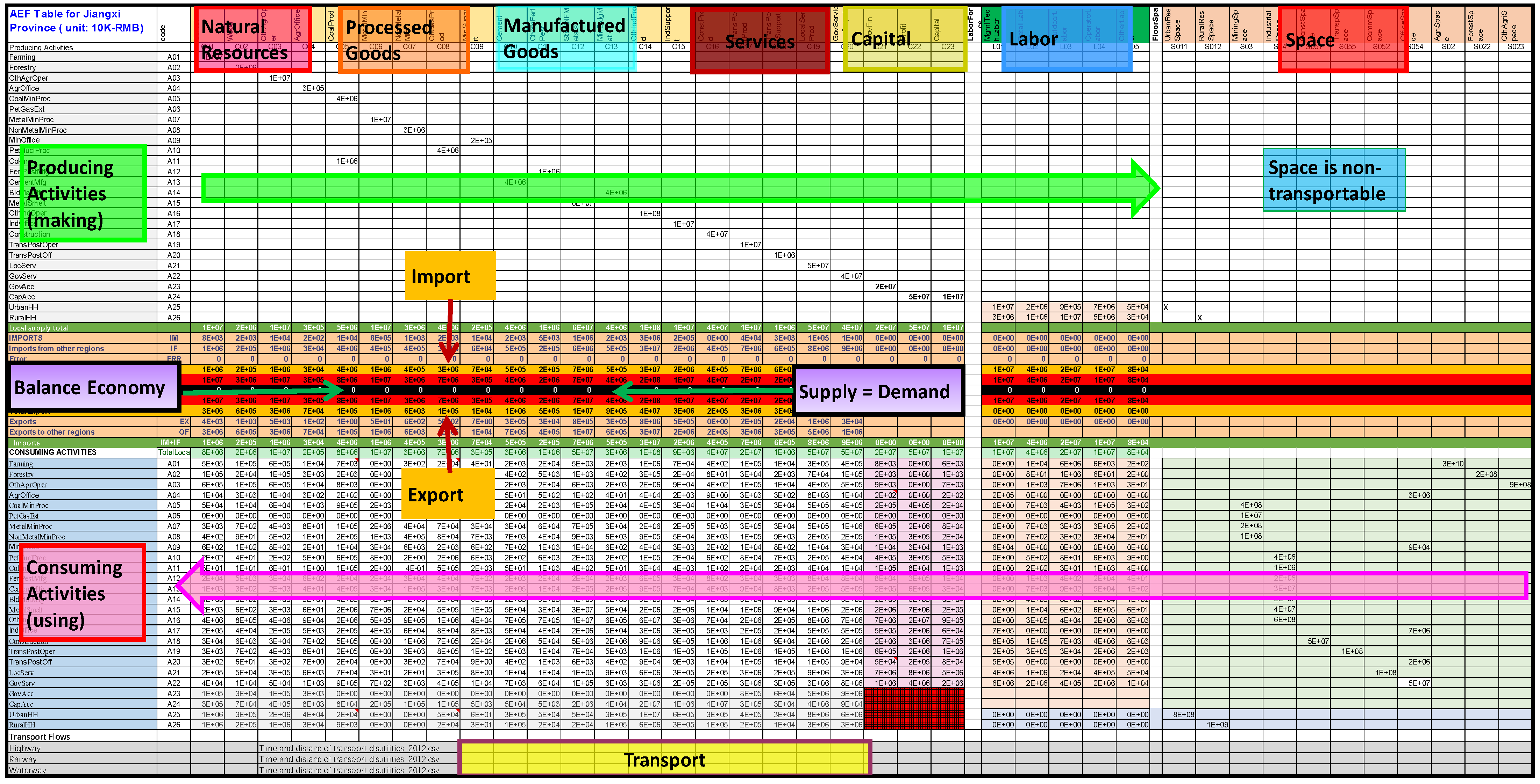
2.1. Development of Aggregate Economic Flow Table

The AEF table, also referred to as the social accounting matrix, is a vital tool for evaluating and analyzing interactions among economic activities, such as industries, non-profit institutions, governments, and households [32,33,34]. This table provides a comprehensive overview of total production, consumption, imports, exports, and intersectoral flows [33]. These flows are determined through TCs or demand functions extracted from the AEF tables, which serve as a basis for projecting passenger and goods flow. The data from the AEF table were used to facilitate economic and demographic forecasting and the development of DSAA methods. Various data sources are used to construct an AEF table, such as IO tables, surveys of households, census data, and space inventories.

2.2. Analytical Framework for Identifying Regional Technology Pattern Disparity

To explore disparities in technology patterns across regions, this study employs a systematic analytical framework comprising three primary steps. First, TCs were calculated for the different regions within a study area. Second, statistical tests were conducted to assess whether there were variations in technology patterns among the various activities and regions. This step is critical for identifying the heterogeneity in technological structures and establishing a foundation for further analysis. Third, the K-means clustering algorithm was used to group sectors and regions based on their TCs. By grouping regions and sectors with similar technological patterns, this approach highlights disparities in technology utilization and provides a detailed understanding of interregional dynamics, as illustrated in Figure 2, which was developed using Microsoft Visio version, 2108.

2.2.1. Technical Coefficients for Different Regions

The calculation of TCs is an important step in the proposed DSEM framework as it elucidates the technological patterns among various regions. In this study, the main IO tables were redesigned according to the required sectors or activities, as mentioned in Appendix A.1 Figure A1, and their TCs (representing the technology used) were calculated for each specific planning unit or area. TCs are typically derived by dividing the value of each input (in monetary terms) by the total output or production of each sector, thereby quantifying the input requirements per unit of output [32,35]. Mathematically, the technical coefficient $a_{ij}$ indicates the quantity of output of sector i absorbed by sector j per unit of total output j, as defined in Equation (1).

$$a_{ij}={\displaystyle \frac{z_{ij}}{x_j}},0<a_{ij}<1$$

(1)

where

—

$z_{ij}$ is the input from industry i to industry j.

—

$x_j$ is the total output of industry j.

2.2.2. Gini Index

The Gini index is used to measure the differences or sectoral changes in TCs between two different periods in the IO table [36]. This approach enables to quantify the degree of stability or volatility in the production structures of different sectors over time. By comparing the Gini indices for these periods, significant changes in sectoral production processes can be identified, indicating stability or transformation within sectors. To this end, the two distributions of TCs (corresponding to the two years) for each column j are ranked according to the value of ${\phi }_{ij}$, as specified in Equation (2).

$${\phi }_{ij}={\displaystyle \frac{a_{ij}^t}{a_{ij}^{t+n}}}$$

(2)

A value of $a_{ij}^t/a_{ij}^{t+n}$ of less than 1 indicates an increase in TCs over time, whereas a value greater than 1 suggests a decrease. Following this ranking, the cumulative sums of the normalized coefficients for each year were computed. These cumulative coefficients,${\mathrm{F}}_{\mathrm{k}}$ and ${\mathrm{G}}_{\mathrm{k}}$ were used to calculate the Gini index for sector j, as presented in Equations (3)–(5).

$${\mathrm{F}}_{\mathrm{k}}={\sum }_{\mathrm{i}=1}^{\mathrm{k}}\left({\mathrm{a}}_{\mathrm{i}\mathrm{j}}^{\mathrm{t}+\mathrm{n}}/{\sum }_{\mathrm{i}=1}^{\mathrm{N}}{\mathrm{a}}_{\mathrm{i}\mathrm{j}}^{\mathrm{t}+\mathrm{n}}\right)$$

(3)

$${\mathrm{G}}_{\mathrm{k}}={\sum }_{\mathrm{i}=1}^{\mathrm{k}}\left({\mathrm{a}}_{\mathrm{i}\mathrm{j}}^{\mathrm{t}}/{\sum }_{\mathrm{i}=1}^{\mathrm{N}}{\mathrm{a}}_{\mathrm{i}\mathrm{j}}^{\mathrm{t}}\right)$$

(4)

$${\mathrm{G}\mathrm{i}\mathrm{n}\mathrm{i}}_{\mathrm{j}}^{\mathrm{t},\mathrm{t}+\mathrm{n}}=\sum _{\mathrm{i}=1}^{\mathrm{N}-1}{\mathrm{F}}_{\mathrm{i}}\cdot {\mathrm{G}}_{\mathrm{i}+1}-\sum _{\mathrm{i}=1}^{\mathrm{N}-1}{\mathrm{F}}_{\mathrm{i}+1}\cdot {\mathrm{G}}_{\mathrm{i}}$$

(5)

where

—

${\mathrm{a}}_{\mathrm{i}\mathrm{j}}^{\mathrm{t}}$ = TCs for one period.

—

$a_{ij}^{t+n}$ = TCs in second period.

—

N = number of sectors.

A higher value of the Gini index indicates greater dispersion and change in TCs for sector j between the two periods, whereas lower Gini values suggest more stability in the sector’s production processes.

2.2.3. K-Means Clustering

This study further employed the K-means clustering algorithm to group activities with similar TCs and patterns across regions, thereby reducing the computational burden, enhancing accuracy, and decreasing time [37,38]. Recognized for its simplicity and effectiveness, K-means clustering excels at uncovering meaningful structures within datasets, thereby facilitating the extraction of insightful groupings of observations [39]. One of the main advantages of K-means clustering over hierarchical clustering is its ability to handle large datasets more effectively. Hierarchical methods, while useful for a small-scale analysis, tend to be computationally intensive and less scalable as the volume of data increases. In contrast, K-means clustering is significantly faster, making it well-suited for regional analysis where large amounts of data, such as regional economic patterns, need to be processed. Density-based spatial clustering of applications with noise (DBSCAN’s) reliance on density-based criteria can make it difficult to obtain consistent results in regions where spatial data points are not uniformly distributed. In contrast, K-means clustering provides a more predictable and clearer framework for clustering, particularly when dealing with large, structured datasets [37,40].

Numerous studies have employed K-means clustering to analyze regional disparities and development patterns across various data attributes [41,42,43,44]. For instance, Kallingal and Firoz [45] utilized K-means clustering to assess interregional disparities in Kerala, India. In practice, the K-means algorithm operates by assigning a predefined number of clusters, denoted as K, which is particularly beneficial when structuring complex datasets, such as regional TCs. This predetermined number of clusters simplifies the analysis and interpretation of data compared to methods such as DBSCAN, which do not require the number of clusters to be specified but can struggle when data density varies. Following several recent studies [46,47], this study adopted the elbow method to determine the optimal K-value for clustering provinces and sectors. The elbow method identifies the point at which the within-cluster sum of squares (WCSS) or inertia decreases sharply, indicating the most appropriate number of clusters [48,49,50]. Beyond this point, increasing k yields no substantial improvement in inertia, ensuring that the clusters maintain their maximum internal homogeneity. This method was implemented in Python 3.8. using standard clustering packages [46]. Compared to other K-value selection techniques, such as the Gap Statistic and Silhouette Coefficient, the elbow method offers a computationally efficient and intuitively interpretable solution, especially when the inflection point on the WCSS curve is distinct [46,47,49].

Once ‘k’ is determined, it proceeds through two main phases.

• Initialization: Randomly select ‘k’ cluster centers.
• Assignment and Update: Assign each data point to the nearest cluster center based on the Euclidean distance and recalculate the cluster centers as the mean of the assigned points. This iterative process is repeated until the change in the cluster centers becomes negligible, thereby minimizing the WCSS.
• The WCSS, a key metric in K-means, measures the squared error between each data point and its corresponding cluster center by summing these across all clusters (Equation (6)).

$$\mathrm{W}\mathrm{C}\mathrm{S}\mathrm{S}=\sum _{i=1}^k\sum _{x\in C_i}{\left|x-x_i\right|}^2$$

(6)

• Euclidean distance plays a critical role in determining the proximity of data points to cluster centers. This measure determines the shortest path between a given data point and the cluster center. For the two vectors the Euclidean distance, denoted as, $\mathrm{d}\left({\mathrm{x}}_{\mathrm{i}},{\mathrm{y}}_{\mathrm{i}}\right)$ was calculated using Equation (7).

$$\mathrm{d}\left({\mathrm{x}}_{\mathrm{i}},{\mathrm{y}}_{\mathrm{i}}\right)={\left[\sum _{i=1}^n{\left(x_i-y_i\right)}^2\right]}^{{\displaystyle \frac{1}{2}}}$$

(7)

2.3. Economic and Demographic Forecast Model

The EDF model constitutes the first component within the DSEM framework. This model forecasts socioeconomic and demographic activities in each planning unit by using the logistic growth (S-curve) method [12,51]. The S-curve method is particularly effective for modeling the evolution of economic activities over time, as it captures typical patterns of regional development. These patterns generally exhibit an initial phase of slow growth, followed by a period of rapid expansion, a subsequent decline in growth rate, and ultimately stagnation [51].

In instances where the S-curve method is unsuitable, owing to the nature of the activity data, the Exponential Smoothing method is employed. Exponential Smoothing is a widely recognized forecasting technique for a time-series analysis [12], which calculates smoothed values based on an exponential function and combines these with a well-defined time-series forecasting model to predict future trends based on present data [51]. The S-curve and Exponential Smoothing methods were calibrated using panel IO data from 2007 to 2017. These methods were subsequently utilized to forecast the activity totals for each province from 2018 to 2050. This study also addressed data anomalies, including missing values, outliers, and extreme observations, using data synthesis, exogenous factors, and imputation techniques. Gross domestic product (GDP) growth rates and total output values from the IO table were used to align the data with regional activity trends [52]. The mathematical formulations for the S-curve and Exponential Smoothing methods are provided in Equation (8) and Equation (9), respectively. Both methods were executed using Python 3.8. [12,52].

$${\widehat{y}}_{\varnothing ,\tau }^t={\displaystyle \frac{K}{1+e^{\mathsf{\alpha }+\mathsf{\beta }\mathrm{t}}}}$$

(8)

where

—

${\widehat{y}}_{\varnothing ,\tau }^t$ = forecasted total for economic activity type $\varnothing$ (where $\varnothing$ = 1, 2…n, e.g., farming, forestry) in province $\tau$ at time $t$.

—

K is the asymptote of the logistic function representing the maximum carrying capacity of the corresponding activity (where K > 0).

—

$\mathsf{\alpha }$ is the growth rate parameter.

—

β is the inflection point, which is the time at which the growth rate is highest (midpoint of the S-curve).

—

$t$ is the time variable (e.g., years from the start of the forecast period).

$${\widehat{y}}_{\varnothing ,\tau }^t=\theta \times y_t+\left(1-\theta \right)y_{\varnothing ,\tau }^{t-1}$$

(9)

where

—

${\widehat{y}}_{\mathrm{\varnothing },\tau }^t$ = forecasted total for economic activity type $\mathrm{\varnothing }$ in province $\tau$ at time $t$,

—

$y_t$ = observed value at current time point $t$,

—

${\stackrel{`}{y}}_{\mathrm{\varnothing },\tau }^{t-1}$ = forecasted value for activity type $\mathrm{\varnothing }$ in province $\tau$ from the previous time point $t-1$,

—

$\theta$ = smoothing constant, with values between 0 and 1, determining the weight assigned to the observed data versus the previous forecast.

2.4. Differential Spatial Activity Allocation Method

The DSAA method aims to evaluate the optimal location for production and consumption activities and their interactions based on a more reasonable assumption of differentiated technology patterns over different areas of a region. This approach, as opposed to the traditional ways in which they are allocated to entire regions using the same technology index, ignores regional disparity in technology distribution. The DSAA considers the number of activities, movement of commodities, and markets, which include total demand and supply, along with exchange prices. This method uses a three-level nested logit framework to reflect the hierarchical and interrelated nature of the decision-making processes in economic activities. Specifically, the nested structure enables the model to jointly capture conditional dependencies among three key decisions (i) where to locate activities, (ii) what type of technology to use, and (iii) where to procure inputs and sell outputs. By allowing for correlated unobserved factors within each decision nest, the nested logit model effectively addresses the interdependence of these choices, enhancing behavioral realism compared with simple multinomial logit models.

2.4.1. Production Activity Allocation

The highest level of the nested logit model allocates the overall activity quantities across specific regional zones (Equations (10) and (11)). The activity forecasts using the EDF method are then passed as inputs to the DSAA method, which further allocates the activity totals to specific regional zones based on the defined parameters and constraints.

$$W_{a,z}={\mathit{T}}_{\mathit{a}\mathsf{\zeta }}\cdot \left({\displaystyle \frac{\mathrm{e}\mathrm{x}\mathrm{p}\left({\lambda }_{1,a}\cdot L{U}_{a,z}\right)}{\sum _{z\in Z}\mathrm{e}\mathrm{x}\mathrm{p}\left({\lambda }_{1,a}\cdot L{U}_{a,z}\right)}}\right)$$

(10)

where

$$\begin{array}{rr}& L{U}_{a,z}={\alpha }_{\mathrm{sizc},a}\cdot {\displaystyle \frac{1}{{\lambda }_{1,a}}}\cdot \mathrm{l}\mathrm{n}\left({\mathrm{Size}}_{a,z}\right)+{\alpha }_{\mathrm{inert},a}\cdot \mathrm{l}\mathrm{n}\left({\mathrm{PrevW}}_{a,z}+{\mathrm{InertCons}}_a\right)\hfill \\ & +{\mathrm{Const}}_{a,z}+{\displaystyle \sum _{v\subset V}}\left({\alpha }_{a,v}\cdot X_{v,z}\right)+{\alpha }_{\mathsf{\Delta }\mathrm{tech},a}\cdot {\mathrm{CUTech}}_{a,z}\hfill \end{array}$$

(11)

where $W_{a,z}$ represents the quantity of activity $a$ allocated to a specific zone z, and $T_{a\mathsf{\zeta }}$ is the total quantity of activity $a$. The location utility for a unit of activity $a$ in zone $z, \left(L{U}_{a,z}\right)$ is calculated as a combination of various factors. The first term—the size term (${\alpha }_{\mathrm{size},a}\cdot {\displaystyle \frac{1}{{\lambda }_{1,a}}}\cdot \mathrm{l}\mathrm{n}\left({\mathrm{S}\mathrm{i}\mathrm{z}\mathrm{e}}_{a,z}\right)$)—captures the size effect, where ${\mathrm{Size}}_{a,z}$ represents the relative attractiveness of zone z for activity a, based on floor space or land use capacity, and ${\lambda }_{1,a}$ indicates the dispersion parameter in the utility function governing the allocation of activity a across zones. In the second term, ${\alpha }_{\mathrm{inert},a}\cdot \ln \left({\mathrm{PrevW}}_{a,z}+{\mathrm{InertCons}}_a\right)$, ${\mathrm{PrevW}}_{\mathrm{a},\mathrm{z}}$ represents the proportion of the total quantity of activity a in a specific zone $\mathrm{z}$ from the previous time period and ${\mathrm{InertCons}}_a$ represents the coefficient that modifies the sensitivity to the prior distribution of activity a across zones, particularly when the previous quantities are small. This controls the degree of “inertia” in the system. ${\mathrm{Const}}_{a,z}$ capture alternative-specific fixed effects. The summation term $\sum _{v\subset V}\left({\alpha }_{a,v}\cdot X_{v,z}\right)$ accounts for other zone-level attributes $X_{v,z, }$ such as infrastructure or accessibility, with ${\alpha }_{a,v}$ indicates their relative importance. Finally, the term ${\alpha }_{\mathsf{\Delta }\mathrm{tech},a}\cdot {\mathrm{CUTech}}_{a,z}$ represents the influence of composite utility from the differential production technology options available in zone z, with ${\alpha }_{\mathsf{\Delta }\mathrm{tech},a}$ measuring sensitivity to technology suitability.

2.4.2. Differential Technology Allocation

The middle level distributes activity quantities within each regional zone among various cluster-based technology options, which determine the production and consumption rates of commodities. Each technology option represents a distinct production and consumption rate for different commodities (goods, services, labor, capital, and floor space), which is derived from the AEF table (Equations (12)–(15)).

$${\mathrm{T}\mathrm{e}\mathrm{c}\mathrm{h}}_{p^{\prime },a,z}=W_{a,z}\times \left({\displaystyle \frac{\exp \left({\lambda }_{p^{\prime },a}\cdot \mathsf{\Delta }{\mathrm{UTech}}_{p^{\prime },a,z}\right)}{\sum _{p^{\prime }\in P_a}\exp \left({\lambda }_{p^{\prime },a}\cdot \mathsf{\Delta }{\mathrm{U}\mathrm{T}\mathrm{e}\mathrm{c}\mathrm{h}}_{p^{\prime },a,z}\right)}}\right)$$

(12)

$$\begin{array}{c}\mathrm{with}:\\ \mathsf{\Delta }{\mathrm{UTech}}_{p^{\prime },\mathit{a},\mathit{z}}={\displaystyle \frac{1}{{\lambda }_{p,a}}}\cdot \ln \left(\left.{\mathrm{O}\mathrm{p}\mathrm{S}\mathrm{i}\mathrm{z}\mathrm{e}}_{p^{\prime },a}\right)\right.+{\mathrm{UProd}}_{p^{\prime },a,z}+{\mathrm{UCons}}_{p^{\prime },a,z}\end{array}$$

(13)

$${\mathrm{Uprod}}_{p^{\prime },a,z}=\sum _{p^{\prime }}{\mathrm{Rate}}_{p^{\prime },a}\times {\mathrm{Scale}}_{p^{\prime },a}\times {\mathrm{CUSell}}_{c,p^{\prime },z}$$

(14)

$$\begin{array}{c}\\ {\mathrm{Ucons}}_{p^{\prime },a,z}={\displaystyle \sum _{p^{\prime }}}-{\mathrm{Rate}}_{p^{\prime },a}\times {\mathrm{Scale}}_{p^{\prime },a}\times {\mathrm{CUBuy}}_{c,p^{\prime },z}\end{array}$$

(15)

where ${\mathrm{T}\mathrm{e}\mathrm{c}\mathrm{h}}_{p^{\prime },a,z}$ is the quantity of activity $a$ in zone z applying differential cluster-based technology option $p^{\prime }$, $W_{a,z}$ is the total activity $a$ in zone $z; {\lambda }_{p^{\prime },a}$ is the utility function dispersion parameter, $\mathsf{\Delta }{\mathrm{U}\mathrm{T}\mathrm{e}\mathrm{c}\mathrm{h}}_{p^{\prime },a,z}$ is the differential cluster-based technology utility, ${\mathrm{O}\mathrm{p}\mathrm{S}\mathrm{i}\mathrm{z}\mathrm{e}}_{p,a}$ is the relative size of the technology option for activity a, and ${\mathrm{UProd}}_{p^{\prime },a,z}$ represents the utility derived from the production and consumption of commodities, respectively, by activity a in zone z, using technology. ${\mathrm{Rate}}_{p^{\prime },a,n}$ is the rate at which commodity c is produced (positive) or consumed (negative) by an activity using technology option $p^{\prime }$. ${\mathrm{Scale}}_{p^{\prime },a}$ is the scaling factor that adjusts the magnitude of the production or consumption rates. Similarly, ${\mathrm{CUSell}}_{c,p^{\prime },z}$ and ${\mathrm{CUBuy}}_{c,p^{\prime },z}$ represent the utility associated with selling and buying a unit of commodity c in zone z.

The production and consumption of commodities in a specific zone are modeled by aggregating contributions from activities and their associated technology options.

This composite utility for applying a range of technology options for activity a in zone z, denoted as ${\mathrm{CUTech}}_{a,z}$ (Equation (16)), is derived based on Equations (12) and (13) and is expressed as follows:

$${\mathrm{CUTech}}_{a,z}=\left(1/{\lambda }_{p^{\prime },a}\right)\cdot \mathrm{l}\mathrm{n}\left[\sum _{p^{\prime }\in P_a}\mathrm{e}\mathrm{x}\mathrm{p}\left({\lambda }_{p^{\prime },a}\cdot {\mathsf{\Delta }UTech}_{p^{\prime },a,z}\right)\right]$$

(16)

This composite utility incorporates the utilities of both buying, $CUBu{y}_{c,z}$, and selling, ${\mathrm{CUSell}}_{c,z}$, the commodities that are used and produced by the technologies applied in the activity. Equation (16) combines these individual utilities to establish the overall composite utility for the technology options ${\mathrm{CUTech}}_{a,z}$. The location utility of an activity is significantly influenced by the composite utility of buying commodities it consumes or selling the commodities it produces. Thus, the final term in Equation (11), ${\mathrm{CUTech}}_{a,z}$, provides a comprehensive measure of the zone’s accessibility to the activity given the technology options applied in that zone.

2.4.3. Production and Consumption Quantities (Exchange Locations)

The quantity of commodity c produced in zone z by activity a is the sum of the quantities produced by each technology option over the set of technology options employed by activity $a$. This is expressed as follows:

$$TP{A}_{c,a,z}=\sum _{p^{\prime }\in P_a}\sum _{p^{\prime }\in P_a\mid {\mathrm{Rate}}_{p^{\prime },a,}>0,c_{p^{\prime }}=c}{\mathrm{Rate}}_{p^{\prime },a}\times {\mathrm{Tech}}_{p^{\prime },a,z}$$

(17)

where

$TP{A}_{c,a,z}$ is the quantity of commodity c produced in zone z by activity a aggregated over all technology options.

The total quantity of commodity c produced in zone z by all activities is the sum of the quantities of commodity c produced over the set of activities, as follows:

$$T{P}_{c,z}=\sum _{a\subset A}TP{A}_{c,a,z}$$

(18)

where $T{P}_{c,z}$ is the quantity of commodity c produced by all activities in zone z, using all technology options. Similarly, the quantity of commodity c produced in zone z by activity a is the sum of the quantities consumed by each technology option over the set of technology options applied by activity a as follows:

$$TC{A}_{c,a,z}=\sum _{p^{\prime }\in P_a}\sum _{p^{\prime }\in P_a\mid {\mathrm{Rate}}_{p^{\prime },a}>0,c_{p^{\prime }}=c}{-\mathrm{Rate}}_{p^{\prime },a}\times {\mathrm{Tech}}_{p^{\prime },a,z}$$

(19)

where

—

$TC{A}_{c,a,z}$ is the quantity of commodity $c$ consumed in zone $z$ by activity $a$, aggregated over all technology options.

The quantity of commodity c consumed in zone z by all activities is the sum of commodities c consumed over the set of activities, as follows:

$$T{C}_{c,z}=\sum _{a\subset A}TC{A}_{c,a,z}$$

(20)

where $T{C}_{c,z}$ is the quantity of commodity c consumed by all activities in zone z, using all the technology options.

Buying and Selling Allocation

The lowest level allocates commodities among the exchange locations (location-specific markets for commodities) where they are bought and sold. This involves two logit allocations per commodity in each zone: one for buying and one for selling. The ${\mathrm{B}}_{\mathrm{c},\mathrm{z},\mathrm{k}}$ refers to the volume of commodity $c$ purchased from an exchange location (a location-specific market for commodities) k to zone $z$, while ${\mathrm{S}}_{\mathrm{c},\mathrm{z},\mathrm{k}}$ refer to the volume of commodity $c$ sold to exchange location $k$ from zone $z$. The allocation of production and consumption quantities is steered by the buying and selling of the utilities of the exchange location $k$, which reflects the ease of obtaining and selling commodities. These utilities are denoted by $\mathrm{B}{U}_{c,z,k}$ and $S{U}_{c,z,\mathrm{k}}$ for buying and selling commodity $c$ from zone $z$ to exchange place $K$ respectively. The allocation process was formalized and computed using Equations (21) and (22), incorporating dispersion coefficients ($\lambda b_c$ and $\lambda s_c)$ that regulate the sensitivity of the buying and selling utility.

$${\mathrm{S}}_{\mathrm{c},\mathrm{z},\mathrm{k}}={\mathrm{T}\mathrm{P}}_{\mathrm{c},\mathrm{z}}\cdot {\displaystyle \frac{\exp \left(\lambda {\mathrm{s}}_{\mathrm{c}}\cdot S{U}_{c,z,\mathrm{k}}\right)}{{\mathsf{\Sigma }}_{\mathrm{k}\mathrm{e}\mathrm{k}}\exp \left(\lambda {\mathrm{s}}_{\mathrm{c}}\cdot {\mathrm{S}\mathrm{U}}_{\mathrm{c},\mathrm{z},\mathrm{k}}\right)}}$$

(21)

$${\mathrm{B}}_{\mathrm{c},\mathrm{z},\mathrm{k}}={\mathrm{T}\mathrm{C}}_{\mathrm{c},\mathrm{z}}\cdot {\displaystyle \frac{\exp \left(\lambda {\mathrm{b}}_{\mathrm{c}}\cdot B{U}_{c,z,k}\right)}{{\mathsf{\Sigma }}_{\mathrm{k}\mathrm{e}\mathrm{K}}\exp \left(\lambda b_c\cdot B{U}_{c,z,k}\right)}}$$

(22)

The utilities associated with buying and selling commodities are influenced by key factors, such as the exchange price $\left({\pi }_{c,k}\right),$ transportation cost $\left({TC}_{c,z,k}\right),$ and production ${(q}_{c,k})$ or consumption scales $\left({\overline{q}}_{c,k}\right)$. These factors are reflected in the buying utility $B{U}_{c,z,k}$ or selling utility $S{U}_{c,z,\mathrm{k}}$, as defined in Equation (23) and Equation (24), respectively. The sensitivity of the buying utility to these factors is characterized by the coefficients ${\delta }_{\mathrm{price},\mathrm{c}}^{\mathrm{b}}, {\delta }_{\mathrm{tran},\mathrm{c}}^{\mathrm{b}}, {\mathrm{a}\mathrm{n}\mathrm{d} \delta }_{\mathrm{size},c}^{\mathrm{b}},$ which correspond to the influence of exchange price, transportation cost, and market scale, respectively. Similarly, the coefficients ${\delta }_{\mathrm{price},c}^{\mathrm{s}}, {\delta }_{\mathrm{tran},\mathrm{c}}^{\mathrm{s}}, {\mathrm{a}\mathrm{n}\mathrm{d} \delta }_{\mathrm{size},c}^{\mathrm{s}}$ represent the effects of these factors on the selling utility.

$$B{U}_{c,z,k}={\delta }_{\mathrm{p}\mathrm{r}\mathrm{i}\mathrm{c}\mathrm{e},c}^{\mathrm{b}}\times {\pi }_{c,k}+{\delta }_{\mathrm{t}\mathrm{r}\mathrm{a}\mathrm{n},c}^{\mathrm{b}}\times {TC}_{c,z,k}+{\delta }_{\mathrm{s}\mathrm{i}\mathrm{z}\mathrm{e},c}^{\mathrm{b}}\times {\displaystyle \frac{1}{\lambda b_c}}\times \ln {(q}_{c,k})$$

(23)

$$S{U}_{c,z,\mathrm{k}}={\delta }_{\mathrm{price},c}^s\times {\pi }_{c,k}+{\delta }_{\mathrm{tran},c}^s\times {TC}_{c,z,k}+{\delta }_{\mathrm{size},c}^s\times {\displaystyle \frac{1}{\lambda s_c}}\times \ln \left({\overline{q}}_{c,k}\right)$$

(24)

The solution algorithm of the DSAA method incorporates a set of nonlinear constraints to achieve equilibrium between supply and demand across the exchange zones. The DSAA method uses several key input parameters to adjust and improve the model’s performance. These parameters include dispersion parameters for buying (${\lambda }_b^c$) and selling $({\lambda }_s^c$) from the nested logit model, constants of the logit model, and option weights that adjust the sizes of technology options (${\mathrm{O}\mathrm{p}\mathrm{S}\mathrm{i}\mathrm{z}\mathrm{e}}_{p,a}$) within the DSAA method. These parameters were adjusted iteratively to ensure that the model is closely aligned with the base-year production data, as accurately as possible. The aggregate demand for each commodity c in each exchange zone k is the total quantity of the commodity bought in the exchange zone, including the internal bought quantity and export quantity in the zone. The quantity of commodity c exported from exchange zone k to external regions, denoted as $Q{i}_{c,k}$. The aggregate demand $\left({\mathrm{T}\mathrm{D}\mathrm{e}\mathrm{m}}_{\mathrm{c},\mathrm{k}}\right)$ for each commodity c in the exchange zone k is calculated using Equation (25).

$${\mathrm{T}\mathrm{D}\mathrm{e}\mathrm{m}}_{\mathrm{c},\mathrm{k}}=Q{e}_{c,k}+{\sum }_{z\in Z}{\mathrm{B}}_{\mathrm{c},\mathrm{z},\mathrm{k}}$$

(25)

Similarly, the quantity of commodity c, imported from external regions to exchange location k, is denoted as $Q{i}_{c,k}$. The aggregate supply $\left({\mathrm{T}\mathrm{S}\mathrm{u}\mathrm{p}}_{\mathrm{c},\mathrm{k}}\right)$ for commodity c in exchange zone k is the total quantity sold, including internal sales and imports. This is defined in Equation (26).

$${\mathrm{T}\mathrm{S}\mathrm{u}\mathrm{p}}_{\mathrm{c},\mathrm{k}}=Q{i}_{c,k}+{\sum }_{z\in Z}{\mathrm{S}}_{\mathrm{c},\mathrm{z},\mathrm{k}}$$

(26)

The algorithm strives for equilibrium by progressively modifying the exchange prices in each zone until a market balance is achieved. The equilibrium condition is satisfied when aggregate supply equals aggregate demand for all commodities and exchange zones, as shown in Equation (27).

$${\mathrm{T}\mathrm{E}}_{\mathrm{c},\mathrm{k}}={\mathrm{T}\mathrm{D}\mathrm{e}\mathrm{m}}_{\mathrm{c},\mathrm{k}}={\mathrm{T}\mathrm{S}\mathrm{u}\mathrm{p}}_{\mathrm{c},\mathrm{k}}$$

(27)

where ${\mathrm{T}\mathrm{E}}_{\mathrm{c},\mathrm{k}}$ = is the exchange quantity for commodity c in exchange zone k.

${\mathrm{Residual}}_{\mathrm{c},\mathrm{k}}$ between the supply and demand are calculated as:

$${\mathrm{Residual}}_{\mathrm{c},\mathrm{k}}={\mathrm{TSup}}_{\mathrm{c},\mathrm{k}}-{\mathrm{TDem}}_{\mathrm{c},\mathrm{k}}$$

(28)

In theoretical equilibrium, these residuals should be zero. However, to maintain the computational efficiency, the iterative process was terminated when the residual values fell within a predefined convergence threshold. The DSEM algorithm iteratively adjusts exchange prices to minimize residual imbalances and achieve a market equilibrium. Price changes in each zone are computed based on the partial derivatives of the total excess demand (the surplus of demand over supply) with respect to the prices in the respective zone. Cross-zone and cross-commodity price interactions are assumed to have negligible effects and are excluded from derivatives. A step adjustment factor enhances convergence by dynamically adapting the magnitude of price changes. If the price adjustment reduces excess demand, the factor is slightly increased in the subsequent iterations. Conversely, if the excess demand increases, the adjustment is reversed, the factor is significantly reduced, and a smaller adjustment is applied. This ensures a more efficient refinement of the equilibrium and improves the predictive accuracy of the model. The iterative process typically requires 3000 iterations to converge, during which allocations are updated based on current prices, and prices are revised in response to the resulting supply and demand levels.

Upon convergence, the DSAA method outputs include exchange prices, commodity flows, floor space predictions, and activity allocation forecasts. The commodity flows are stored as an Open Matrix (OMX) and integrated with Cube Voyager software for further analysis. The monetary flows in the OD matrices are converted into tonnage, which is then loaded onto a multimodal transport supernetwork for mode and route choice analyses [53].

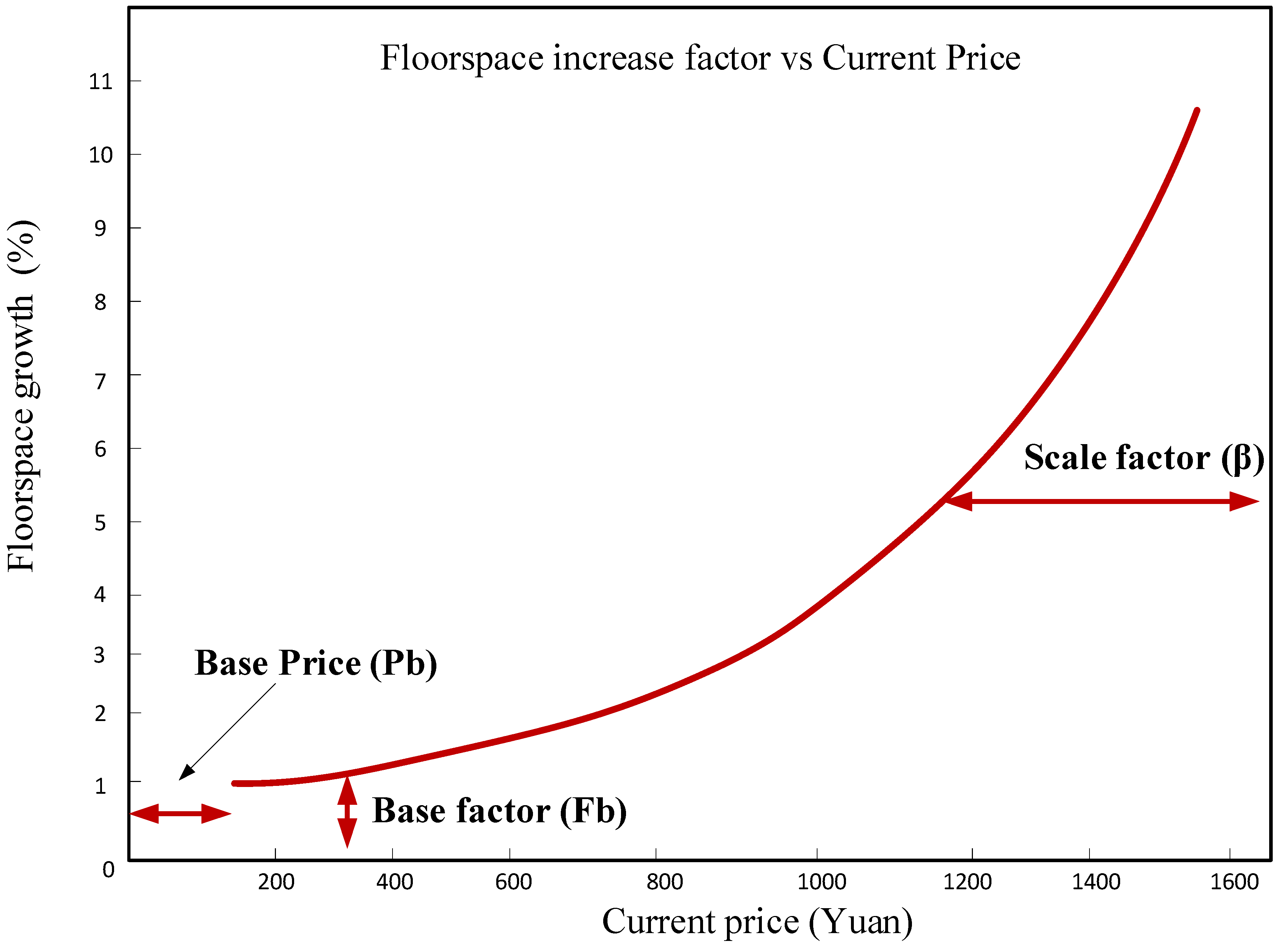
2.5. Space Development Model

Given the long-term and large-scale nature of spatial planning, this study adopts the Aggregate Space Development (ASD) model, which offers greater feasibility from both data availability and engineering perspectives. The ASD model determines the types of space within each TAZ, which were aligned with the administrative boundaries of the districts and counties. These developments were assessed based on key factors, including current (T-year) space quantities, maximum available capacity, and market prices. Based on these inputs, the model projects the quantity of each space type developed in the subsequent year (T + 1) within a given region [12,54,55]. Furthermore, the ASD model leverages remote sensing data to estimate land availability at the county or district level, providing a spatially explicit foundation for modeling. The model forecasts space development by type for future years, factoring in the interplay between the available land (floor space) and market prices (Equation (29)).

$$F=F_b+\exp \left({\displaystyle \frac{P\ast \beta -P_b}{P_b}}\right)$$

(29)

where F represents the factor applied to the current floor space and Fb denotes the base factor. P refers to the current price, $P_b$ represents base price, and β is the scale factor used for adjustment. The Fb is the foundational level of the adjustment to floor space, while the scale factor (β) determines the smoothness of percentage growth. Both parameters are calibrated to values between 0 and 1 (

Table 1. Parameter calibration results of aggregate space development function.

Space Code	Space Name	Current Price	Base Factor	Scale Factor
S011	UrbanResSpace	220	0.2	0.7
S012	RuralResSpace	220	0.2	0.7
S03	MiningSpace	300	0.2	0.5
S04	IndustrialSpace	300	0.2	0.5
S051	ConstSpace	300	0.2	0.5
S055	TranspSpace	300	0.2	0.5
S052	CommSpace	600	0.3	0.7
S054	OfficeSpace	400	0.3	0.6
S021	AgriSpace	23	0.1	0.4
S022	ForestSpace	23	0.1	0.4
S023	OthAgriSpace	23	0.1	0.4

). The interaction of these parameters produces a growth curve (Figure 3) that aligns with observed trends, ensuring realistic projections.

The ASD model is calibrated by adjusting the parameters (Fb, β, P, Pb) based on observed data until the estimated growth curve mirrors the trend of the observed curve. This process ensures that the model’s projections are reliable and aligned with historical and current market dynamics [27].

Based on the observed data of built-up areas, including industrial, commercial, and residential spaces, within the YREB, the values of the parameters in Equation (29) were determined (Table 1).

2.6. Integrated Multimodal Freight Assignment Based on a Supernetwork

This study develops a transport model for a large-scale region, incorporating a multimodal transport supernetwork consisting of highways, railways, and waterways. A supernetwork is a comprehensive representation of multimodal transportation systems that encompasses both physical components, such as highways, railways, and waterways, and virtual components, including transfer links, TAZ centroids/hub connector links, and hubs/TAZ centroids [56]. Spatial OD allocation is performed using a probit-based stochastic user equilibrium assignment model [12,57], which allows the distribution of commodity OD trip matrices generated by the DSAA method onto the multimodal network. This approach contrasts with traditional FSM model because it eliminates the assumption of independent transport modes, avoids the artificial segmentation of transportation processes, and allocates commodities by type with a focus on primary goods within the study area. This methodology ensures that the model delivers highly detailed and accurate data, thereby providing essential insights into the transportation planning and infrastructure development.

This study used an integrated transport network impedance function based on generalized costs to evaluate the total link costs for different transport modes. The generalized cost function calculates the total cost of transporting goods between nodes i and j using a specific transport mode m. It incorporates various cost components, including base transportation costs, transshipment costs, loading costs, transfer costs, travel time, transfer time, and opportunity costs due to increased travel time (e.g., caused by congestion) from the perspective of freight carriers. Additionally, it accounts for unobservable factors represented by an alternative-specific constant (ASC). The generalized cost function is given by Equation (30).

$$\begin{array}{ll}& C_{ij}^{(c,r)}={\sum }_{(a,b)}^d\left(t_{ij}^{(c,r)}\times {\mathrm{L}\mathrm{F}}_{(a,b)}^c\right)+{\sum }_{(k,l)}^N\left(t_{ij}^{(c,r)}\times L_{(k,l)}^{\mu }\times {\mathrm{B}\mathrm{T}\mathrm{F}}^{(c,\mathsf{\mu })}\right)+{\sum }_{(a,b)}^d\left(t_{ij}^{(c,r)}\times {\mathrm{T}\mathrm{F}\mathrm{R}}_{(a,b)}^c\right)\\ & +t_{ij}^{(c,r)}\times {\mathrm{V}\mathrm{P}\mathrm{T}}^c\times {\displaystyle \frac{{\mathrm{R}\mathrm{O}\mathrm{R}}_t}{365\times 24}}\times \left[{\sum }_{(a,b)}^d\left({\mathrm{L}\mathrm{T}}_{(a,b)}^c\right)+{\sum }_{k,l}^N{TT}_{(k,l)}^{(c,\mu )}+{\sum }_{(a,b)}^d\left({\mathrm{T}\mathrm{T}\mathrm{R}}_{(a,b)}^c\right)\right]+\mathrm{A}\mathrm{S}\mathrm{C}\end{array}$$

(30)

where

—

$C_{ij}^{c,r}$: Total cost (RMB) of transporting commodity $c$ from TAZ $i$ to $TAZ j$ via route $r$.

—

${\mathrm{LF}}_{a,b}^c$: Loading fee $\left({\displaystyle \frac{\mathrm{R}\mathrm{M}\mathrm{B}}{\mathrm{t}\mathrm{o}\mathrm{n}}}\right)$ for commodity $c$ at transfer link $(a,b)\in d$. Note: d is the set of all transfer links, either highway-to-waterway or highway-to-railway.

—

$t_{ij}^{c,r}$: Weight of transporting commodity c from TAZ $i$ to $TAZ j$ in tons via route r.

—

$L_{k,l}^m$: Length (km) of road or rail link $(k,l)$ for mode $\mu , \mathrm{w}\mathrm{h}\mathrm{e}\mathrm{r}\mathrm{e} \mathrm{l}\mathrm{i}\mathrm{n}\mathrm{k} (k,l)\in N$.

—

${\mathrm{B}\mathrm{T}\mathrm{F}}^{c,\mu }:$ Base travel cost per kilometer in $\left({\displaystyle \frac{\mathrm{R}\mathrm{M}\mathrm{B}}{\mathrm{K}\mathrm{m}·\mathrm{t}\mathrm{o}\mathrm{n}}}\right)$ for transporting commodity $c$ via mode $\mu$. Note: $\mu$ = 1,2,3 for highway, railway, and waterway, respectively.

—

${\mathrm{T}\mathrm{F}\mathrm{R}}_{a,b}^c:$ Transfer cost $in \left({\displaystyle \frac{\mathrm{R}\mathrm{M}\mathrm{B}}{\mathrm{t}\mathrm{o}\mathrm{n}·\mathrm{K}\mathrm{m}}}\right)$ of commodity $c$ at link $\left(a,b\right).$

—

${\mathrm{V}\mathrm{P}\mathrm{T}}^c$: Value of commodity $c$ per ton.

—

${\mathrm{R}\mathrm{O}\mathrm{R}}_t$: Annualized rate of return.

—

${LT}_{a,b}^c$: Loading time (h) for commodity $c$ at links $(a,b)$.

—

${TT}_{k,l}^{c,\mu }:$ Travel time (hour) on $(k,l)$ for mode $\mu$.

—

${TTR}_{a,b}^c:$ Transfer time (hour) at link $\left(a,b\right).$

—

ASC: Alternative-specific constant representing unobservable factors.

—

N denotes the total number of links (k,l) and d represents the sum of the transfer links (a,b), where n,d ∈ r.

Using the probit-based stochastic assignment method, the probability that path $r$ is chosen for a trip from origin $i$ to destination $j$ is given by:

$$P_{ij}^r=P\left(C_{ij}^{c,r}<C_{ij}^{c,q},\forall r\ne q\right)$$

(31)

where $C_{ij}^{c,r}$ is the generalized cost for path $r$ and $C_{ij}^{c,q}$ is the perceived travel cost for any other path $q$.

Once the route choice probabilities are determined, the flow demand $Q^{ij}$ assigned $f_k^{ij}$ to each route k between origin i and destination j is computed as:

$$f_k^{ij}=P_r^{ij}\cdot Q^{ij}$$

(32)

—

$f_k^{ij}$ is the flow assigned to route between origin i and destination j,

—

Qij is the total freight demand (or total flow) from origin i to destination j.

The total flow $x_a$, is computed by summing the flows of all the routes. The link flow is given by:

$$x_a=\sum _{\left(r,s\right)}\sum _{k\in K}{\delta }_{ak}\cdot f_k^{ij}$$

(33)

where

—

$x_a$: Flow on link $a$,

—

${\delta }_{ak}$: binary indicator, 1 if link $a$ is part of route $k,0$ otherwise.

Coefficient of determination: The coefficient of determination (R²) quantifies how well the predicted values align with the observed data, reflecting the proportion of variance in the observed data explained by the model (Equation (34)).

$$R^2=1-{\displaystyle \frac{{\sum }_{i=1}^n{\left(y_i-{\stackrel{`}{y}}_i\right)}^2}{{\sum }_{i=1}^n{\left(y_i-\stackrel{⃐}{y}\right)}^2}}$$

(34)

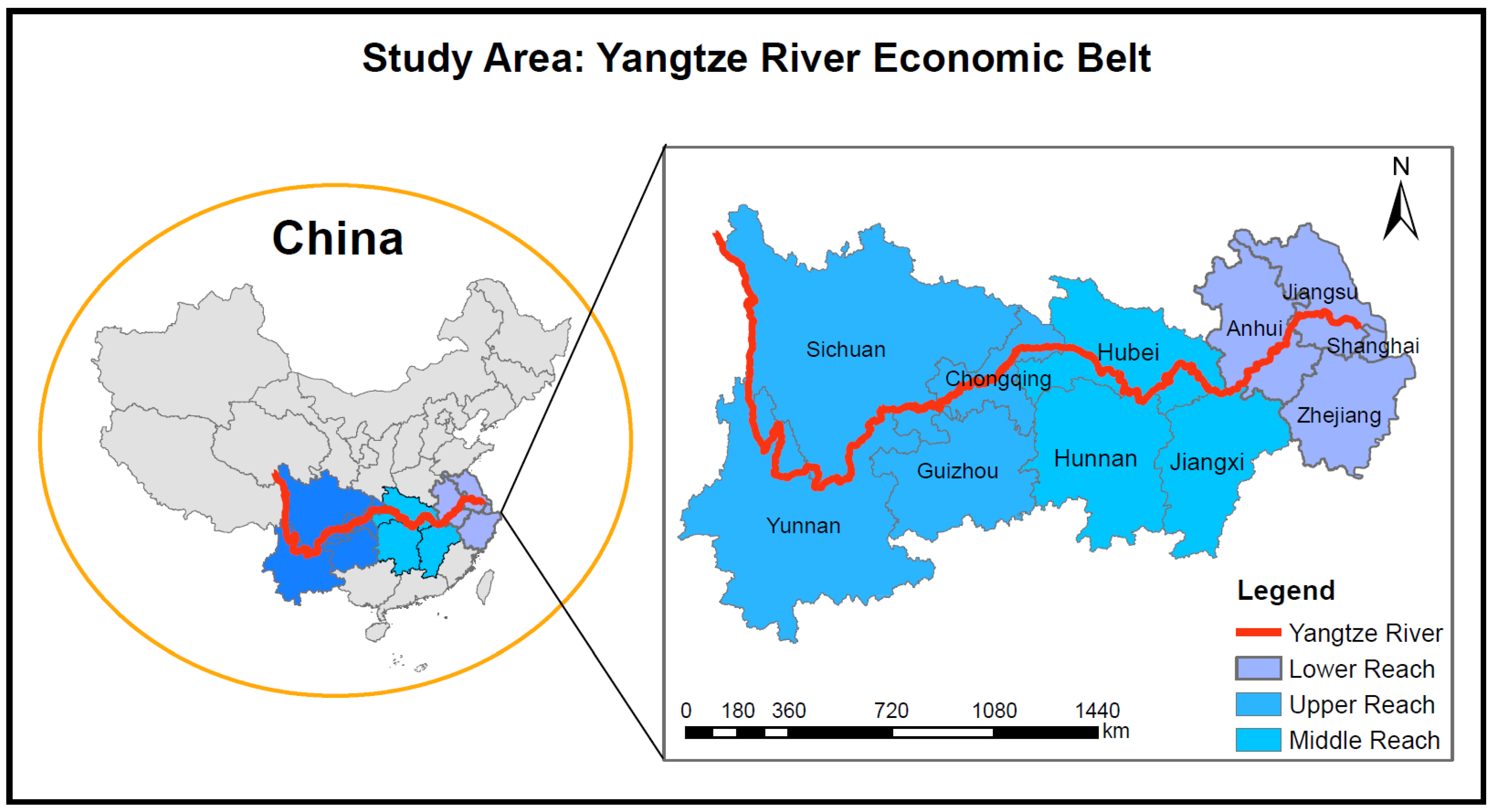
3. Study Area and Data Preparation

This study uses the YREB as a case study. The YREB, which spans nine provinces and two municipalities across 6300 km and 2,552,300 km², is a vital economic region with abundant resources, a strategic location, high population density, and thriving industries. The Yangtze River connects several urban clusters, including the YREB provinces, which are classified into upper, middle, and lower reaches. According to the 2021 China Statistical Yearbook, the YREB comprises 21.5% of China’s territory, 43% of its population, and 46.4% of its gross domestic product (GDP). However, uneven regional development has led to spatial concentrations, inequality, varied regional challenges, emission patterns, and increasing disparities. These issues have intensified the calls for integrated land use and transportation planning. In the recent years, several transportation infrastructure development problems have been identified in China, including overbuilt infrastructure, duplicated construction, and unreasonable competition. These problems primarily stem from neglecting the local conditions, regional development, integrated planning, and overcapacity tendencies during planning. China’s government has initiated plans to address transportation-land development issues by creating a competitive, integrated, equitable, innovative, and eco-friendly transport system by 2035 and 2050 [28,58]. The study area and GDP per capita of the YREB are shown in Figure 4 and Figure 5, respectively [59]. The YREB TAZs and multimodal transportation networks are shown in Figure 6a and Figure 6b, respectively [59,60,61].

3.1. Data Preparation and Sources

Table 2. Description and sources of data for the development of the DSEM method.

Data Description	Data Source and Level	Timeframe
Economic Data
Provincial Statistical Yearbook (Population statistics, socio-economic data, product proportions).	All YREB regions (including 9 provinces and 2 municipalities). Source: Provincial Statistical Bureaus	2010–2020
Input–Output (IO) tables (139 and 42 activities formats)	All YREB regions (including 9 provinces and 2 municipalities) Source: Department of National Accounts, National Bureau of Statistics, China [59,62,63,64].	1997–2017
Technical coefficients	Calculated using a specific method, as detailed in Section 3.3. All YREB regions (including 9 provinces and 2 municipalities)	2007–2017
Population census data	Urban and rural household and employment data. Source: National Data Website (https://data.stats.gov.cn/, accessed on 4 September 2024).	2010, 2012, 2020
China Labor Statistical Yearbook	Data by labor type (5 types). Source: National Data Website (https://data.stats.gov.cn/, accessed on 4 September 2024).	2012
Interregional IO tables	National Data Website (https://data.stats.gov.cn/, accessed on 4 September 2024).	2012
Socioeconomic and Demographic Activity totals	All YREB regions (including 9 provinces and 2 municipalities)	2012–2050
Wages by Labor Type	Source: industry recruitment information and public reports	2012
Observed Household Labor Force Ratio	Selected from partial counties due to data limitations.	2012
Land Use Data
Land Use TAZ .shp Layer	Source: Chinese Academy of Sciences, Resource and Environmental Science Data Center by county and districts (http://www.resdc.cn, accessed on 4 September 2024)	2012
Land Planning Standards	Divided by land type, obtained from national land resources departments by county and districts	2012–2050
Land Use/Cover Data .shp Layer	Divided by land type, land area data, remote sensing data, and by county and districts. Source: Chinese Academy of Sciences, Resource and Environmental Science Data Center (http://www.resdc.cn, accessed on 4 September 2024)	2012–2050
Total Developable Land Area	Total developable land area by land use type, by county and districts. Source: local government	2012
Floor Area Ratio	Divided by space type (10 types of construction land). Source: reference data from Wuhan by county and districts	2012
Space/land Consumption Coefficients	Divided by space type (urban and rural residential space, employment divided into 11 categories) by county and districts (see Appendix A.1).	2012
Employment Data	Obtained by applying to Provincial Statistical Bureau, used to estimate available land area by county and districts. Source: Provincial Statistical Bureau.	2012
Building Area	Sourced from a recent study [12].	2012
Space Price	Divided by space type, referencing Wuhan’s data by county and district level	2012
Land Use Standards	Includes per capita land usage range, floor area ratio, etc. Source: local government	2012
Remote sensing data by space type	Chinese Academy of Sciences, http://english.igsnrr.cas.cn/, accessed on 4 September 2024).	2012, 2015, 2020
Multimodal Transportation Data
Multimodal Network .shp Layer	Three types: highways, railways, waterways. Source: Chinese Academy of Sciences, Resource and Environmental Science Data Center (http://www.resdc.cn, accessed on 10 April 2025); Openstreet maps (https://planet.openstreetmap.org, accessed on 4 September 2024), ArcGIS online	2012
Hub .shp Layer	Includes train stations, ports, logistics centers, etc. Source: Chinese Academy of Sciences, Resource and Environmental Science Data Center (http://www.resdc.cn, accessed on 4 September 2024)	2012
Freight Shipping Rates	Divided by goods and mode. Road, railway, and waterway industry websites. Sourced from a recent study, calculated by [12].	2012
Freight Value	Divided by the ex-factory price of goods. Source: commodity trading websites, China	2012
Typical Transport Vehicle Load Weight	Divided by truck type, train type, and ship type (different tonnages). Source: domestic survey data, China	2012
Driver Wages	Divided by freight mode. Source: Industry recruitment information, China	2012
Time and Distance Impedance Coefficients	by road link	2012
Observed Average Travel Distance	Selected from partial counties by road link due to data limitations.	2012
Short-Distance Freight Transport Time	Calculated by dividing the shortest distance by free-flow speed, used as input data for AA module	2012
Short-Distance Freight Transport Distance	Based on GIS road network data, used as input for AA module.	2012
Loading/Unloading Rates	Unit cost for loading/unloading by goods and mode. Source: “Road Freight Classification Table” and “Loading/Unloading Fee Table”	2012
Transshipment Rates	Unit cost for transshipment by goods and mode. Source: literature “Research on Multi-modal Transport Path Optimization Based on Transportation Scenario” and “Coal Multi-modal Transport Optimization Considering Externality Costs”.	2012
Hub Waiting Time	Hub waiting time by mode. Source: survey [12]	2012
Transport Mode Capacity	Capacity of road segments by mode and grade. (1) Road: “Road Network Planning, Construction, and Management Methods” (2) Rail: “Discussion on Maximum Load of Single and Double Track Railways”	2012
Annual Average Daily Freight Volume by Mode	Used for model calibration, freight volume by mode. Sourced from a recent study [12]. (1) Road: “China Transportation Statistics Yearbook 2013” (2) Rail: Obtained from railway stations via project support. (3) Water: Ship signature data	2012
Annual Freight Volume by Mode	Source: National Data Network (https://data.stats.gov.cn/, accessed on 15 September 2024)	2012–2018
Annual Freight Turnover by Mode	Source: National Data Network (https://data.stats.gov.cn/, accessed on 15 September 2024)	2012–2021
Mode Share	Used for model calibration and validation. Source: calculated from annual freight volume statistics.	2011–2021
Transport cost (RMB/Km-ton)	Sourced from a recent study [12,65].	2012

shows the key data required for the development of the DSEM framework, including data on the economy, land use/space (including building area and land), and transportation. In terms of the economy, it includes IO tables, provincial statistical yearbooks, population censuses (urban and rural population/employment positions), and so on. Space includes land use, transportation, development, space consumption, land control planning, and floor area ratios. Transportation includes regional GIS data (transportation zones, basic road networks, ports, railway stations, and hubs), historical freight data (port throughput data, traffic statistics yearbooks, and railway station freight connection data), freight rates, cargo values, transport speeds, historical freight volumes, and historical cargo turnover volumes. To ensure the robustness and accuracy of the multimodal transportation supernetwork, a series of validation checks were conducted, focusing on reasonableness, topological integrity, and network connectivity. These checks were essential for developing a reliable network capable of supporting large-scale simulations and modeling.

The validation process included assessments of geo-referencing precision, topological accuracy, and network connectivity to ensure compatibility with real-world transport infrastructure. Missing network links, such as unclassified roads, port access roads, and intermodal connectors, were incorporated to enhance network completeness. Additionally, road sections and nodes were classified to facilitate the integration of freight impedance-related parameters in the subsequent modeling stages.

Topological integrity checks addressed issues such as misconnected/dangling links, undershoots, and overshoots that could affect network stability. Each network link was systematically assigned attributes—including capacity, free-flow speed, and cost structure. Subnetwork connectivity was verified, with anomalies identified and resolved to maintain consistency across transport modes.

Finally, the intermodal connections were carefully structured to reflect realistic freight transport operations. This structured approach ensured an accurate representation of multimodal freight flows within the transportation supernetwork.

3.2. Development of Aggregate Economic Flow Table for YREB

The DSEM method extends the PECAS model to handle specific regions instead of allocating study-wide activities to the entire region, which is considered a strong assumption of homogeneous technology pattern. Therefore, this study develops an independent AEF table for each province or municipality in the YREB. Two types of IO tables are available in China: 139 and 42 activities for the base year 2012. To reconcile and design the AEF table for the DSEM, sectors corresponding to the original 42 activities were used directly, whereas multi-activity sectors were further divided based on the 139 activities outlined in the IO table. This process resulted in 22 activities, 2 financial accounts, and urban and rural households. Additionally, it contained 23 commodities, 5 types of labor, and 11 types of spaces (see Appendix A.1

Table A1. Activities, commodities/services, labor, and space categories in the proposed DSEM Method.

Activities	Short Name and Code	Commodity/Services	Labor	Land/Space
Farming	A01Farming	Cereal	Management, technical labor	Urban residential space
Forestry	A02Forestry	Wood	Retail service labor	Rural residential space
Other Agriculture Operation	A03OthAgrOper	Other farming	Outdoor labor	Mining space
Agriculture-Office	A04AgrOffice	Agriculture support	Operator labor	Industrial space
Coal Mining and Processing	A05CoalMinProc	Coal	Other labor	Construction space
Petroleum and Natural Gas Extraction	A06PetGasExt	Oil, Gas and its product		Transportation space
Metals Mining and Processing	A07MetalMinProc	Metallic mineral		Commercial space/land
Nonmetal Minerals Mining and Processing	A08NonMetalMinProc	Nonmetal mineral		Office space
Mining Office	A09MinOffice	Mining support		Agricultural space
Petroleum and nuclear fuel processing	A10PetNuclProc	Oil, gas, and its product		Forest space
Coking	A11Coking	Coal		Other agricultural space
Fertilizer and pesticide manufacturing	A12FertPestMfg	Chemical fertilizers and pesticides
Cement, lime and gypsum manufacturing	A13CementMfg	Cement
Brick, stone and other building materials manufacturing	A14BldMatMfg	Mineral building materials
Smelting and Processing of Metals (Metal Products)	A15MetalSmelt	Steel and nonferrous metals
Other Industry Operation	A16OthIndOper	Other industrial products
Industry-Office	A17IndOffice	Manufacturing support
Construction	A18Construction	Construction
Transport and Post Operations	A19TransPostOper	Transportation product
Transport and Post Office	A20TransPostOff	Transportation support
Local Services	A21LocServ	Local services product
Government Services	A22GovServ	Government services
Government Accounts	A23GovAcc	Government accounts
Capital Accounts	A24CapAcc	Capital
Household-Urban	A25UrbanHH
Household-Rural	A26RuralHH

and Figure A1). These AEF tables were carefully designed and calibrated because their totals were used to develop EDF and DSAA models.

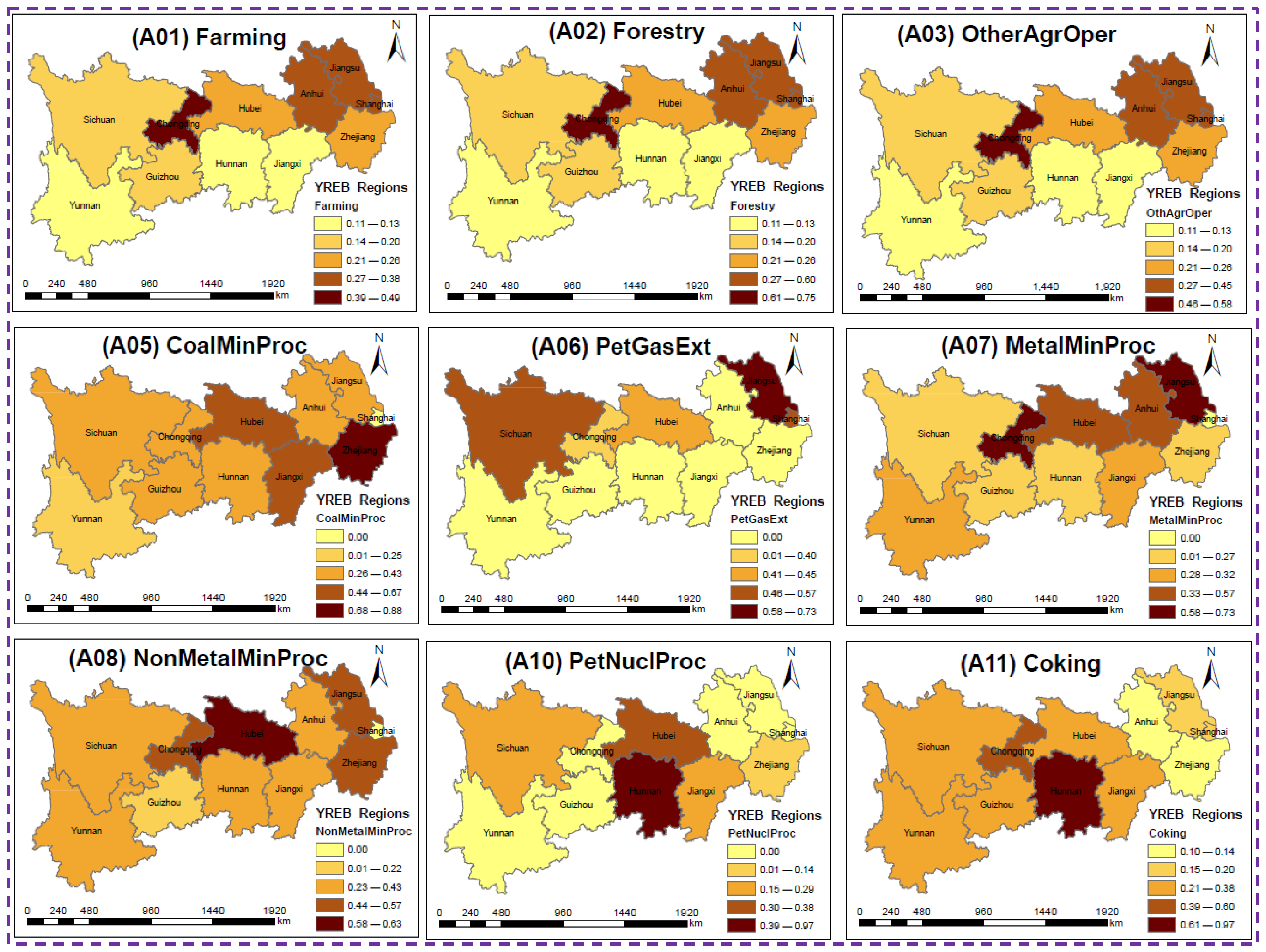
3.3. Calculation of Technical Coefficients

The TCs for various economic activities within each region of the YREB were estimated using provincial IO tables presented in the form of a 22 × 22 activity matrix, as illustrated in Figure 7. These TCs were subsequently utilized for further statistical analyses, including the Gini index, K-means clustering, and DSAA method.

As shown in Figure 7, industrial activities A10 and A11 exhibit high TCs in Shanghai, Zhejiang, Jiangxi, and Hubei, indicating that the production and consumption rates for these activities in these provinces are significantly higher than those in other regions. Conversely, when examining TCs in the aggregated YREB, the overall TCs values were considerably lower. This discrepancy arises because the aggregated values represent an average across all provinces, thereby diluting the impact of provinces where these activities are highly concentrated while also disregarding provinces where these activities may be absent. Consequently, regional disparities in industrial activity intensity were less pronounced in the aggregate TSEM analysis.

4. Case Study Analysis

4.1. Results of Gini Index

The Gini coefficient between 2007 and 2012 (Figure 8) revealed significant variability in TCs across sectors and regions in the YREB, indicating dynamic changes in some areas, while the others remained stable. Figure 8 shows the Gini Index for various sectors across regions, which provides a measure of TC inequality. High Gini values indicate substantial changes in input structures, whereas low values indicate stability [36]. The Gini coefficient analysis for the periods 2007–2012 reveals significant variability in TCs across sectors and regions in the YREB. The Gini index, which ranges from 0 (perfect equality) to 1 (perfect inequality), quantifies the extent of variation in input structures, where high values indicate significant changes and low values suggest stability.

During the 2007–2012 period (Figure 8), substantial disparities were observed in energy-intensive industries, whereas traditional sectors such as agriculture and local services remained relatively stable. The Petroleum and Nuclear Fuel Processing sectors exhibited high Gini values, particularly in Hunan (0.97), Jiangxi (0.29), and Hubei (0.38), suggesting significant changes in the input structures. Notably, this sector was not available in Guizhou, Chongqing, Yunnan, Jiangsu, Anhui, or Shanghai, reinforcing its regional concentration. Similarly, the coal mining and processing sector displayed high Gini values in Hubei (0.67) and Zhejiang (0.88), reflecting shifts in the energy sector structures. The metal mining and processing sector also demonstrated considerable inequality, particularly in Hubei (0.48), whereas the coking sector in Hunan (0.97) exhibited significant changes in the TCs.

The non-metal mineral mining and processing sector reflected notable variability, with Gini values of 0.63 in Hubei and 0.51 in Chongqing, indicating structural shifts in extraction and processing activities. In contrast, sectors such as farming, forestry, and other agricultural Operations maintained low Gini values, suggesting stability in the TCs. For example, Jiangxi (0.11), Hubei (0.26), and Hunan (0.17) exhibited limited changes. Similarly, the local services sector showed minimal variation, with low Gini values in Jiangxi (0.13) and Hubei (0.12), indicating consistency in economic activity. The industrial office sector also displayed stability, with low Gini values in Jiangxi (0.21), Hunan (0.16), and Zhejiang (0.06), reflecting trends in the other industrial operations sectors, where low Gini values in Jiangxi (0.13), Hunan (0.16), and Chongqing (0.10) further support the evidence of sectoral stability.

Importantly, significant changes have been observed in several industries, providing empirical evidence against the hypothesis that TCs remain fixed and homogenous over time. This suggests that the assumption of heterogeneous TCs is empirically supported, and there is a need to embed it in the DSEM model.

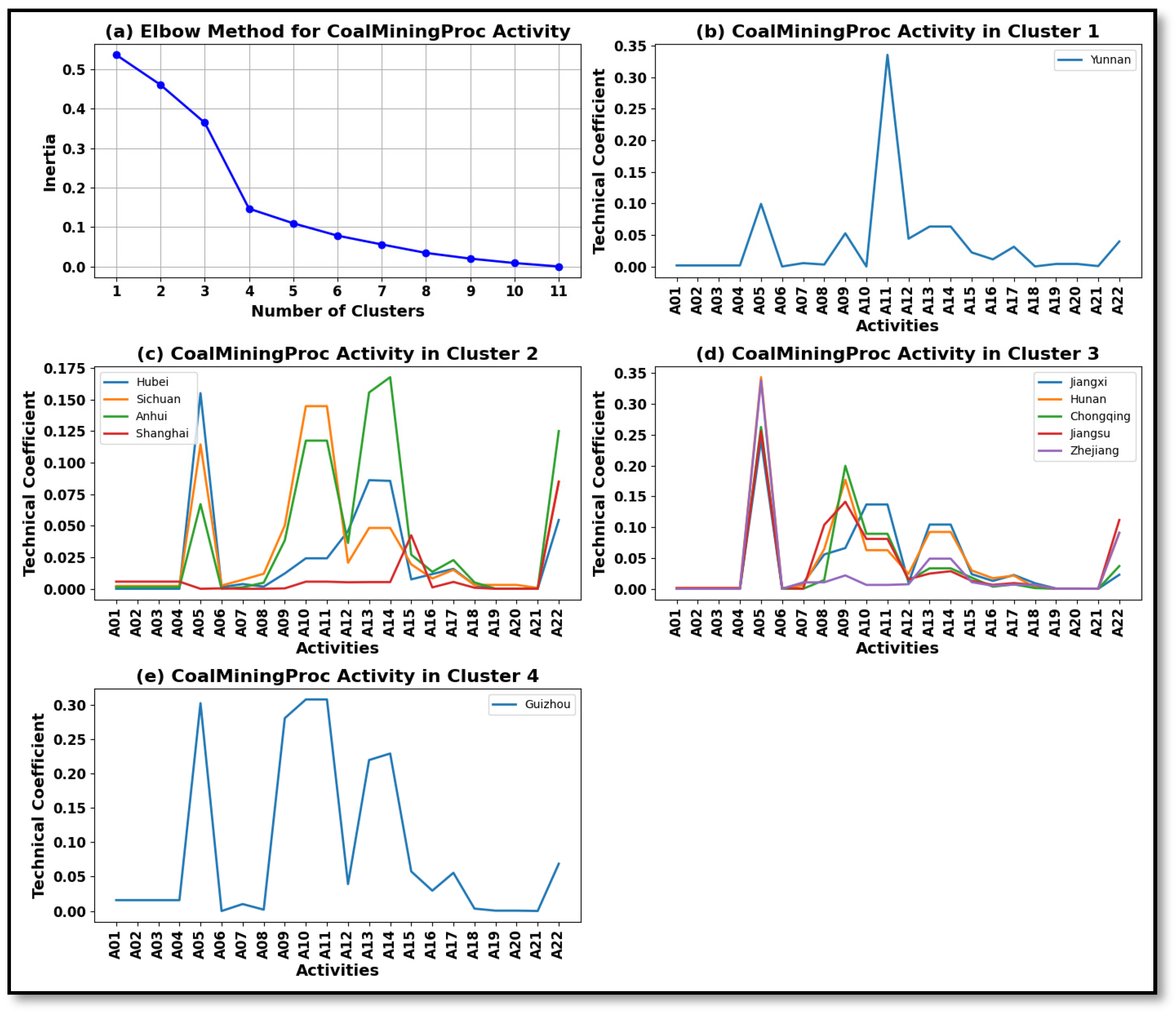
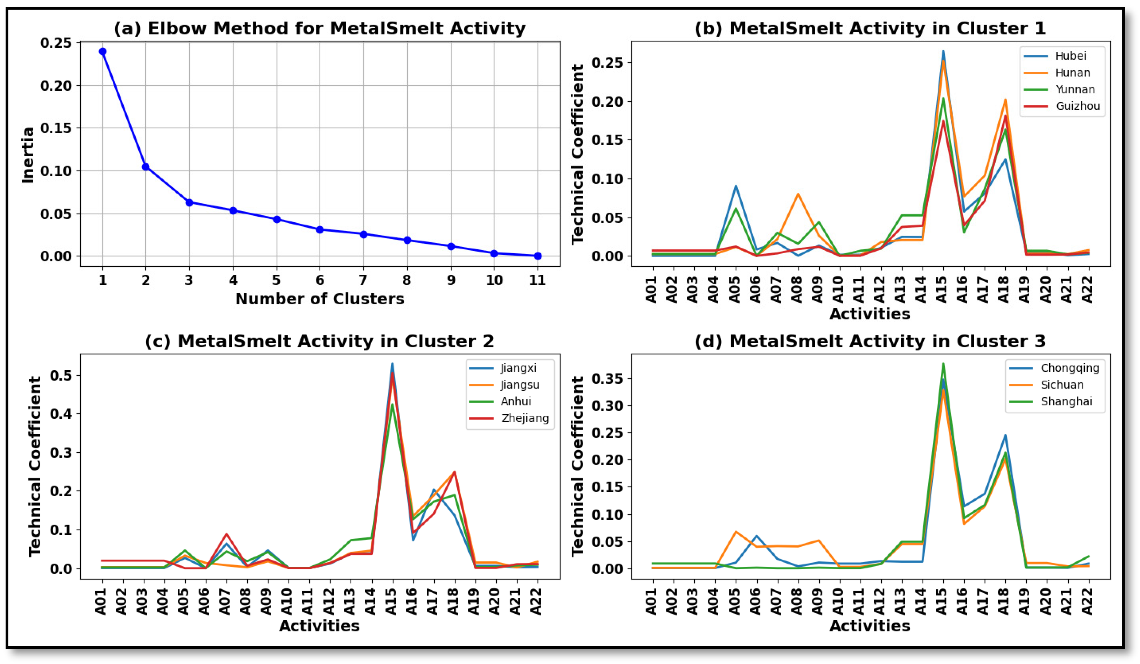
4.2. Results of K-Means Clustering

The K-means clustering analysis revealed different “technology pattern” groups for various activities. Farming and forestry had two clusters, coal mining and processing had four clusters, construction had three clusters, other industrial operations had five clusters, and government services had six clusters (

Table A2. Results of K-means Clustering.

Activities	Cluster 1	Cluster 2	Cluster 3	Cluster 4	Cluster 5	Cluster 6
Farming	Hubei, Hunan, Chongqing, Sichuan, Yunnan, Guizhou, Anhui, Shanghai	Jiangxi, Jiangsu, Zhejiang
Forestry	Hubei, Hunan, Chongqing, Sichuan, Yunnan, Guizhou, Anhui, Shanghai	Jiangxi, Jiangsu, Zhejiang
OthAgrOper	Hubei, Hunan, Chongqing, Sichuan, Yunnan, Guizhou, Anhui, Shanghai	Jiangxi, Jiangsu, Zhejiang
AgrOffice	Hubei, Hunan, Chongqing, Sichuan, Yunnan, Guizhou, Anhui, Shanghai	Jiangxi, Jiangsu, Zhejiang
CoalMinProc	Yunnan	Hubei, Sichuan, Shanghai, Anhui	Jiangxi, Zhejiang, Hunan, Chongqing, Jiangsu	Guizhou
PetGasExt	Jiangxi, Hubei, Jiangsu, Sichuan, Anhui, Zhejiang, Shanghai	Hunan, Chongqing, Yunnan, Guizhou
MetalMinProc	Jiangxi, Hubei, Hunan, Chongqing, Zhejiang	Sichuan, Yunnan, Guizhou, Anhui, Shanghai	Jiangsu
NonMetalMinProc	Jiangxi, Hubei, Hunan, Yunnan, Guizhou, Shanghai	Chongqing, Jiangsu, Anhui, Zhejiang	Sichuan
MinOffice	Jiangxi, Hubei, Hunan, Chongqing, Yunnan, Guizhou	Jiangsu, Sichuan, Anhui, Zhejiang, Shanghai
PetNuclProc	Jiangxi, Hubei, Chongqing, Jiangsu, Sichuan, Yunnan, Guizhou, Anhui, Zhejiang, Shanghai	Hunan
Coking	Jiangxi, Hubei, Chongqing, Jiangsu, Sichuan, Yunnan, Guizhou, Anhui, Zhejiang, Shanghai	Hunan
FertPestMfg	Jiangxi, Guizhou, Anhui, Zhejiang, Shanghai	Hunan, Chongqing, Jiangsu, Sichuan	Hubei, Yunnan
CementMfg	Jiangxi, Hubei, Hunan, Guizhou, Anhui, Shanghai	Chongqing, Jiangsu, Sichuan, Yunnan	Zhejiang
BldMatMfg	Jiangxi, Hubei, Hunan, Jiangsu, Guizhou, Anhui, Zhejiang	Chongqing, Sichuan, Yunnan, Shanghai
MetalSmelt	Hubei, Hunan, Yunnan, Guizhou	Jiangxi, Jiangsu, Anhui, Zhejiang	Chongqing, Sichuan, Shanghai
OthIndOper	Yunnan	Hubei, Hunan, Guizhou, Anhui	Jiangsu, Zhejiang, Shanghai	Chongqing	Jiangxi, Sichuan
IndOffice	Chongqing, Jiangsu, Jiangxi, Anhui, Zhejiang, Shanghai	Hubei, Sichuan, Yunnan, Guizhou	Hunan
Construction	Jiangxi, Hunan, Chongqing, Jiangsu, Sichuan, Guizhou, Anhui, Zhejiang	Yunnan, Shanghai	Hubei
TransPostOper	Jiangxi, Hubei, Hunan, Chongqing, Sichuan, Yunnan, Guizhou, Anhui	Jiangsu, Zhejiang, Shanghai
TransPostOff	Jiangxi, Hubei, Hunan, Chongqing, Sichuan, Yunnan, Guizhou, Anhui	Jiangsu, Zhejiang, Shanghai
LocServ	Jiangxi, Hubei, Hunan, Chongqing, Jiangsu, Sichuan, Yunnan, Guizhou, Anhui, Zhejiang	Shanghai
GovServ	Hunan, Jiangsu, Sichuan, Anhui	Hubei, Guizhou	Chongqing	Zhejiang	Jiangxi, Yunnan	Shanghai

, Appendix A.2). For brevity, only coal mining and processing, smelting and metal processing, and other industrial activities are presented here. The K-means clustering analysis of coal mining and processing activities revealed four distinct clusters based on TCs, as illustrated in Figure 9, which was developed using Python 3.8. The elbow method, illustrated in Figure 9a, indicates that the optimal number of clusters is two, as observed at the inflection point, where the inertia significantly decreases. This suggests that dividing the data into two clusters provides a balance between minimizing within-cluster variance and avoiding unnecessary complexity. Cluster 1 (Yunnan) was uniquely characterized by distinct technical patterns (Figure 9b). Cluster 2 (Hubei, Sichuan, Anhui, and Shanghai) shared similar and moderately high TCs, indicating aligned technological practices (Figure 9c). Cluster 3 (Jiangxi, Hunan, Chongqing, Jiangsu, and Zhejiang) exhibited high TCs, suggesting intensive coal-mining activities (Figure 9d). Finally, Cluster 4 (Guizhou) showed notably high TCs, reflecting a specialized and intensive approach to coal mining (Figure 9e). These clusters reflect the varied technical strategies and resource utilization in coal mining and processing across different provinces.

K-means clustering analysis of metal smelting and processing revealed three distinct clusters based on the TCs (Figure 10a). Cluster 1 (Hubei, Hunan, Yunnan, and Guizhou) exhibited consistent and moderate TCs, indicating similar and moderately intensive metal processing activities (Figure 10b). Cluster 2 (Jiangxi, Jiangsu, Anhui, and Zhejiang) was characterized by higher TCs, reflecting a more intensive and technologically advanced engagement in metal processing (Figure 10c). Cluster 3 (Chongqing, Sichuan, and Shanghai) showed moderate TCs with unique variations, indicating a balanced yet slightly differentiated approach to smelting and processing (Figure 10d). These clusters highlight the diverse technological practices and intensities of metal processing across the regions.

K-means clustering for other industry-operation activities (including universal device, dedicated equipment, transportation equipment, electrical machinery and equipment, communication equipment, computers and other electronic devices, instrumentation, other manufactured products, and waste scrap) revealed five distinct clusters based on the TCs (Figure 11a). Cluster 1 (Yunnan) showed moderate and variable TCs, indicating unique practices (Figure 11b). Cluster 2 (Hubei, Hunan, Guizhou, and Anhui) exhibits consistent and moderately high coefficients, reflecting aligned technological practices (Figure 11c). Cluster 3 (Jiangsu, Zhejiang, and Shanghai) had high TCs, suggesting intensive and advanced industrial operations (Figure 11d). Cluster 4 (Chongqing) had distinct peaks, indicating unique or specialized practices (Figure 11e). Cluster 5 (Jiangxi and Sichuan) showed high variability, reflecting a diverse range of technological practices in other industrial operations (Figure 11f). These clusters highlight the varied technological strategies and intensities of other industrial operations across the regions.

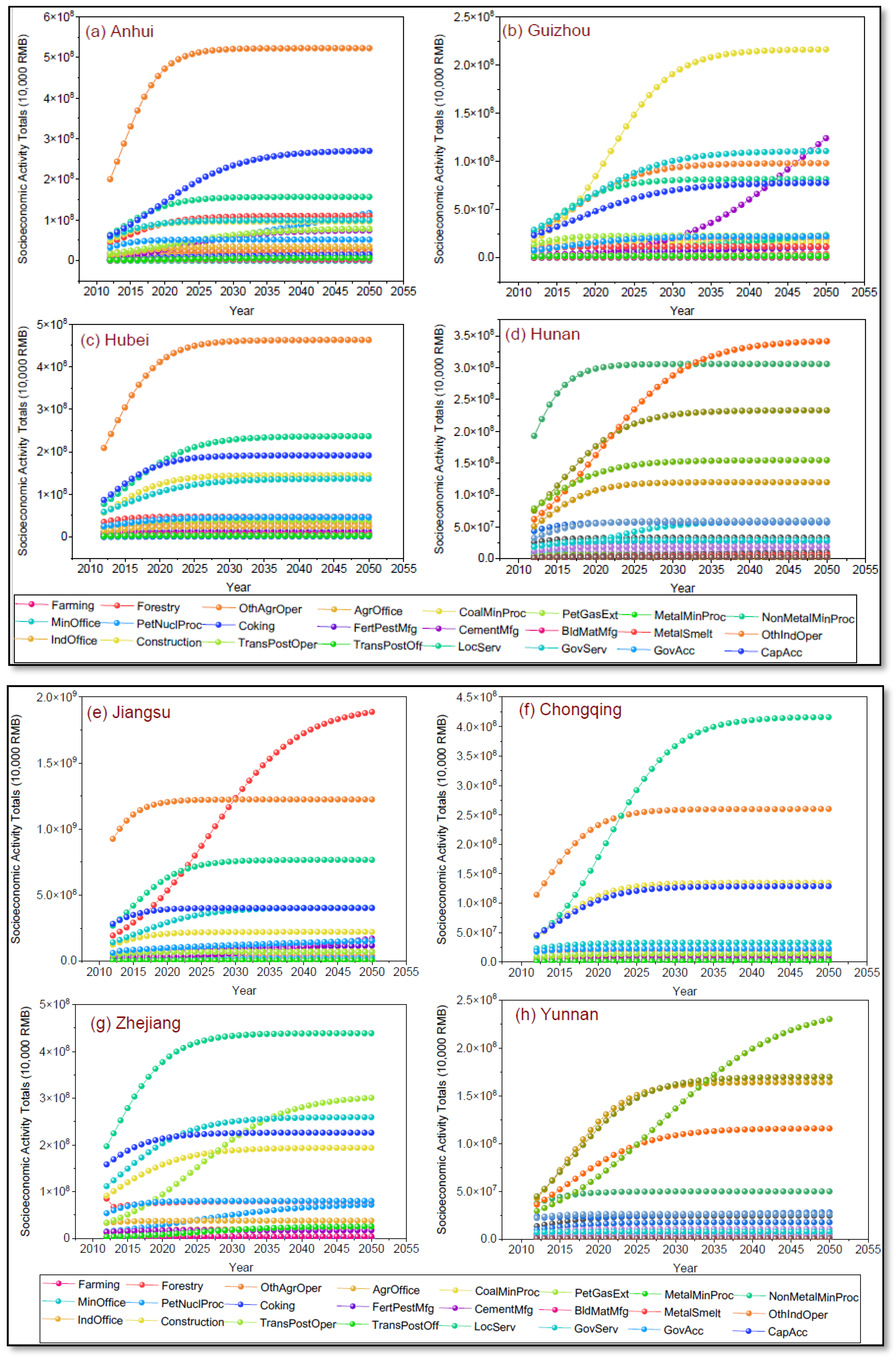
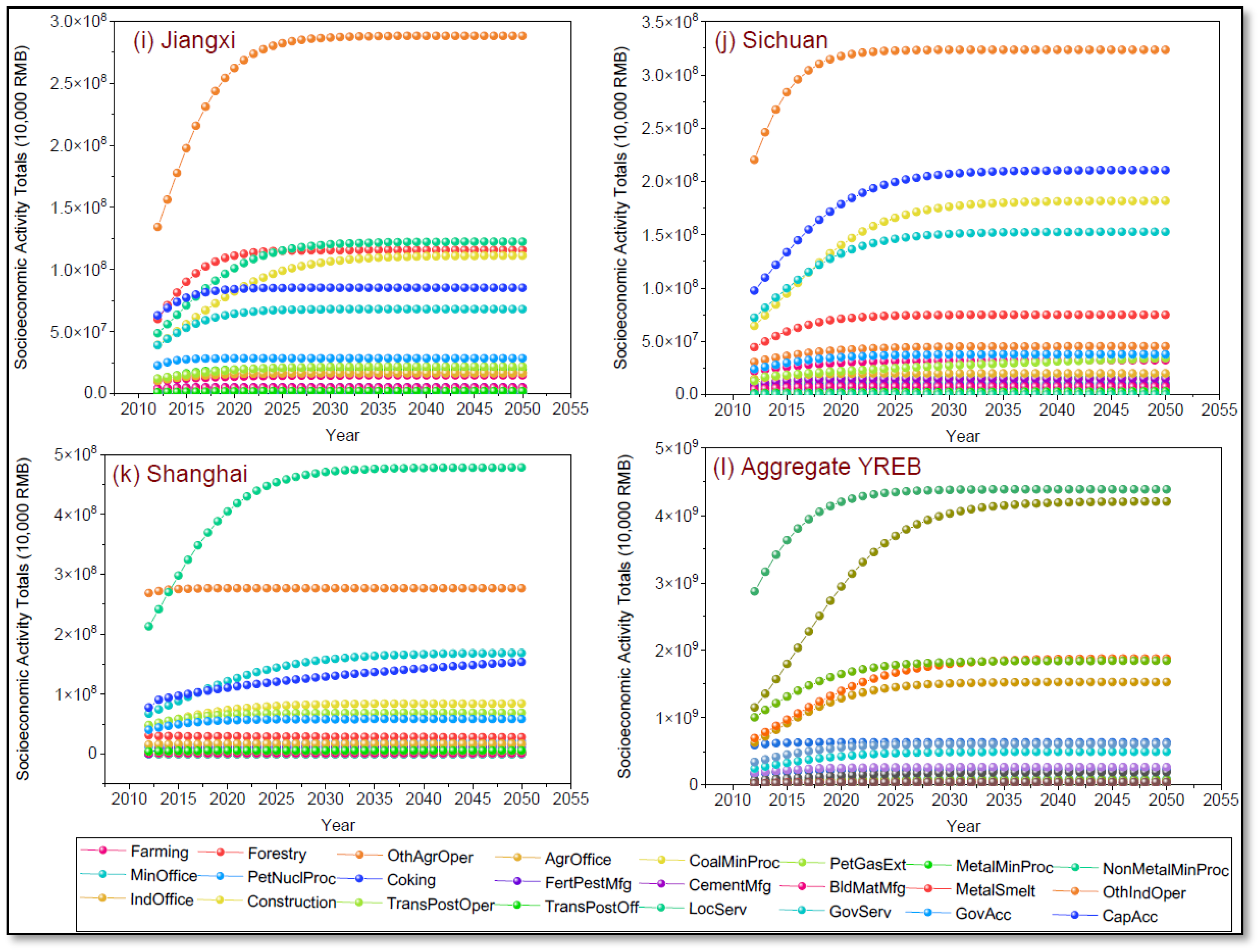
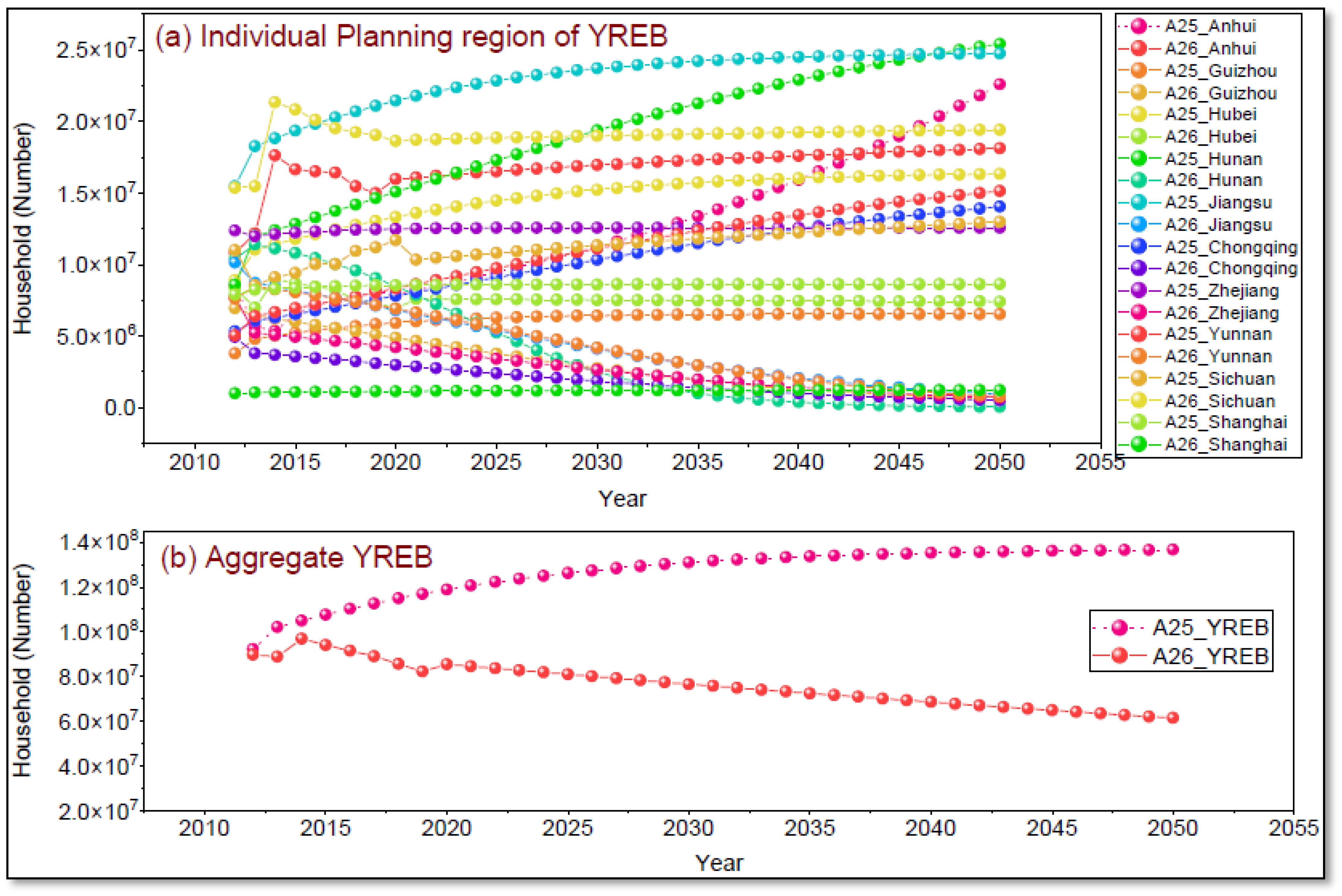
4.3. Results of Economic and Demographic Models

Based on the EDF model outlined in Section 2.3, this study forecasts the socioeconomic and demographic activities in each planning unit using the logistic growth (S-curve) method and Exponential Smoothing method (Figure 12a–l). The results indicate that most activities of IPUs and the YREB follow a logistic S-curve, which aligns with the regional economic development pattern: an initial phase of slow growth, followed by rapid expansion, a deceleration phase, and finally stabilization. This pattern reflects economic progression as sectors mature and structural constraints emerge [12,51].

The upper reaches of the YREB show a higher agricultural growth (an average of 2.44% per year) compared to the middle (1.06% per year) and lower reaches (0.83% per year). Notably, upper-reach provinces have a greater capacity for primary industries. The secondary industry sectors exhibited varied growth across provinces, with rapid construction activity growth rates observed in provinces such as Hunan (3.54%), Anhui (2.40%), Shanghai (2.20%), and Jiangsu (1.99%). These results are consistent with the expected growth rates of the construction industry in China [66,67]. The metal mining and processing industry grows significantly in certain provinces, such as Hubei (1.93% per year) and Sichuan (2.3% per year), while growth is moderate or slow in others, and declines in the lower reaches, particularly in Zhejiang. It is important to note that metal mining and processing activities do not exist in Shanghai [62,63,64]. In addition, the growth rates of non-metal mineral mining and processing activities exhibit moderate trends across the region. Chongqing leads with a growth rate of 4.07%, followed by Jiangsu (2.38%), Anhui (2.10%), and Jiangxi (1.97%). On the other hand, provinces such as Hunan (1.04%), Sichuan (0.91%), and Yunnan (0.87%) show relatively lower growth rates per year. Coal mining and processing have been declining in various provinces. For instance, Hunan (0.29%), Sichuan (0.20%), and Anhui (0.06%) have demonstrated lower growth rates in coal mining and processing. This decline can be attributed to the YREB’s strategic focus on “ecological priority and green development” in the coming years, which promotes secondary and tertiary industries while gradually reducing the polluting industries [27]. In contrast, most tertiary industries, except for mining office services exhibit increasing trends (Figure 12a–l). Demographically, the urban household (A25) population across the YREB is experiencing rapid growth, especially in the upper provinces, reflecting intensified urbanization trends. This result aligns with the previous studies showing that urban density in the upper reaches remains higher than that in the middle and lower reaches [27,68]. Meanwhile, the rural household (A26) population showed a steady decline in all regions, notably in Guizhou, Jiangsu, Zhejiang, Chongqing, and Hunan. This trend aligns with the YREB’s long-term planning objectives, emphasizing the development of urban agglomeration. In addition, the model prediction results are generally in line with the declining trend in China’s total population and rural population [12] (Figure 13a,b).

An analysis of the individual provinces within the YREB revealed that certain economic activities were absent in specific regions. For example, coal mining and processing activities are absent in Shanghai. Similarly, petroleum and natural gas extraction were absent in Jiangxi, Hunan, Guizhou, Yunnan, Anhui, Shanghai, and Zhejiang. Furthermore, petroleum and nuclear fuel processing has not been observed in Guizhou, Chongqing, Yunnan, Jiangsu, Anhui, and Shanghai [62,63,64,69]. Conversely, the aggregated YREB forecast shows cumulative growth rates for these activities, leading to the potential overestimation or underestimation of long-term forecasts for such a large region. This discrepancy arises because the aggregate forecast does not account for the absence of these activities in certain regions, thus skewing the results. In contrast, analyzing individual planning units provides a more objective and accurate representation of regional growth patterns. These findings provide empirical support for the assumption proposed in this study that the growth and development of economic activities are subject to the unique characteristics of each province, including regional, demographic, cultural, natural, geographic, and technological factors [70,71,72]. This finding highlights the need to adopt region-specific policy approaches for industrial development.

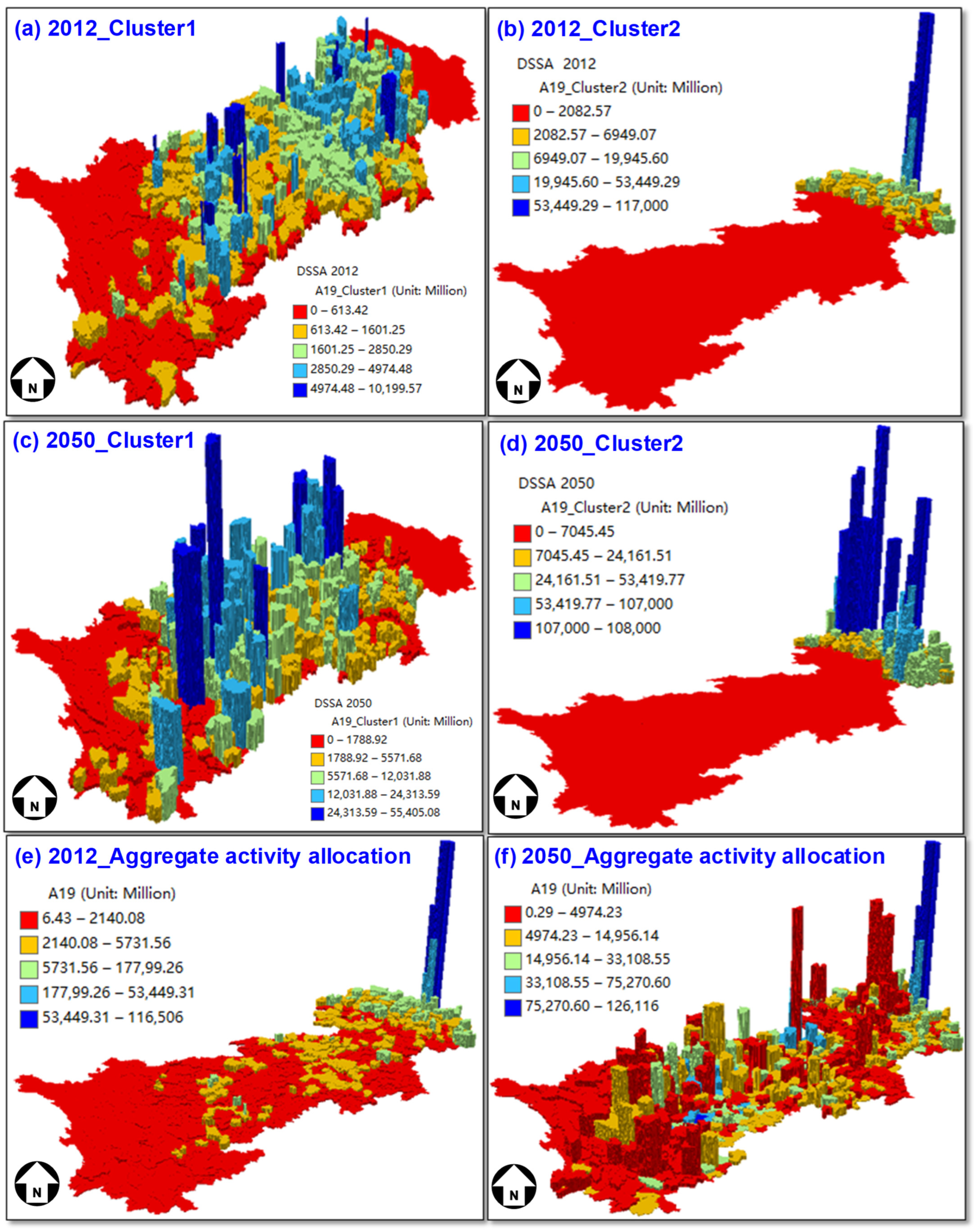
4.4. Results of Differential Spatial Activity Allocation

The DSAA analysis forecasted the spatial distribution of 26 economic activities. For the sake of brevity, we present the results for selected activities, specifically A15—smelting and processing metal products, and A19—transportation operation activity. Figure 14a–f illustrates the results of smelting and metal processing using the proposed DSAA method, revealing interesting regional trends. These figures were developed using ESRI’s ArcScene 10.8. In Cluster 1 (Hubei, Hunan, Yunnan, and Guizhou), faster growth was observed, which may be due to industrial policies and infrastructure development. In Cluster 2 (Jiangxi, Jiangsu, Anhui, Zhejiang), these activities grow more rapidly in Anhui and Jiangsu than in Jiangxi and Zhejiang, indicating a strategic shift to areas with more land and lower labor and material costs. In Cluster 3 (Chongqing, Sichuan, and Shanghai), there was a decline in these activities in Shanghai, which is attributed to limited land and stringent CO₂ reduction goals, prompting relocation to less urbanized areas.

Figure 14g,h compare the DSAA results with aggregate activity allocation, showing the aggregate study-wide smelting and metal product distribution across all zones without considering each planning unit. Most of the activities were allocated to the upper and lower reach areas of the YREB, ignoring the middle reach areas. However, relying on a single technology option for all economic activities can skew the results by focusing on activities in technologically advanced regions and neglecting other zones [12,14]. These results suggest that relocating labor-intensive and high-emission industries to inland areas is a crucial strategy for achieving spatially balanced industrial development. The middle and upper reaches of the YREB, which possess abundant natural resources and a large labor force [12], are well-positioned to accommodate these industries. Furthermore, China’s policy directives emphasize transportation infrastructure development and industrial decentralization as key strategies for promoting regional economic balances [28].

Figure 15a–d depict the results of the allocation of A-19, transportation and postal operations activity, over the TAZs of the modeling region, the YREB, using the proposed method. The findings revealed that in Cluster 1 (Jiangxi, Hubei, Hunan, Chongqing, Yunnan, Sichuan, Guizhou, and Anhui), the trend demonstrated an increasing tendency in the middle-reach areas, and that upper regions of the YREB are expanding more rapidly than the lower regions. In Cluster 2 (Jiangsu, Zhejiang, and Shanghai), transport and logistics activities show strong growth, outpacing other YREB regions, reinforcing the economic advantage and established logistics networks of these provinces. Furthermore, the results were compared to the aggregate activity allocation of construction, which exhibited a nonuniform distribution of A-19 transportation and postal operations activity (Figure 15e,f). The 2012–2050 period exhibits a gradual shift in transportation hubs toward the middle YREB, suggesting an emerging logistics rebalancing strategy that could alleviate transportation bottlenecks and enhance regional connectivity. These results demonstrate that the proposed method can capture area-specific activity growth, providing a rational outcome for policymakers and governments implementing policies for regional balance development.

4.5. Forecast Results of Space Development Distribution

Based on the space development methodology outlined in Section 2.5, this study forecasts the future distribution of space and land development volumes across various socioeconomic sectors. The predicted industrial activity space is shown in Figure 16. Figure 16a–c presents the results of the DSEM model, which restricts space allocation to each planning unit by considering specific regional land availability, growth potential, and unique economic and zoning characteristics. These findings indicate that the model effectively allocates space to IPU within TAZs, aligned with the administrative boundaries of the districts and counties of the YREB. This allocation reflects a realistic and regionally appropriate distribution of industrial land, ensuring that the model captures the local development patterns and constraints. A comparative analysis further underscored these disparities. In 2025, industrial space development using the DSEM model is projected at 165.57 million square meters, whereas the TSEM estimates 206 million square meters. Similarly, for 2035, the DSEM model forecasts 255.77 million square meter, whereas the TSEM projects 354.52 million square meter. By 2050, the DSEM model predicts 407.2 million square meters, whereas the TSEM estimates 577.18 million square meters. The results reveal that the TSEM consistently overestimates space development, failing to account for specific planning unit constraints, leading to less precise spatial allocation (Figure 16d–f). These findings emphasize the superior accuracy of the DSEM model in capturing realistic industrial space development trends. The DSEM aligns with the observed patterns of industrial land expansion and constraints, reinforcing the necessity of incorporating region-specific land use considerations in forecasting methodologies. In contrast, the TSEM’s reliance on aggregate coefficients results in spatial overestimation, underscoring the limitations of models that do not integrate planning-unit constraints in land allocation. Based on the results of the DSEM and TSEM framework (Figure 16) for the period 2025 to 2050, industrial land development in the lower reaches of the YREB—including Shanghai, Zhejiang, Jiangsu, and Anhui—is projected to gradually decline. This is primarily due to the fact that industrial development in these areas has already reached a mature scale, and the diminishing marginal economic benefits have curtailed further expansion [27]. Consequently, the demand for additional industrial land has stagnated. Moreover, limited land availability further restricts the potential for continuous growth. As a result, industrial development is expected to shift progressively toward the upper reaches of the YREB (Yunnan, Guizhou, Sichuan, and Chongqing), where land resources are more abundant and development potential remains higher. This spatial shift aligns with the actual patterns of economic and spatial restructuring observed in the YREB [12,27].

4.6. Forecast Results of Freight Distribution

This study presents a freight distribution forecasting using DSEM frameworks, which replace the traditional trip generation and distribution models. The DSEM method provides a more accurate and realistic representation of freight flows by integrating spatial and economic interdependencies of commodity movements. The OD flows generated by the DSEM are initially represented in monetary units. Commodity-specific conversion factors were used to convert these flows into tonnage-based freight movements [65]. The analysis focused on several key freight commodities, including cereals, wood, agricultural products, coal and its derivatives, metallic and non-metallic minerals (such as salt), oil and gas products, cement, chemical fertilizers and pesticides, steel and non-ferrous metals, mineral-based building materials, and other industrial products. This section emphasizes the results of cereal and coal flows, as these commodities represent the primary focus of the analysis.

The cereal OD matrix, with 1,170,724 records (1082 × 1082), presents a highly detailed and dense dataset. Attempting to visually represent all records would result in overwhelming complexity, with each line corresponding to a single freight movement, making it impossible to infer meaningful patterns. As a result, Wuhan City was selected as a case study for cereal distribution given its significant role in cereal trade in the region.

Figure 17a illustrates the cereal flow forecast based on the DSEM, generated using the Kepler.gl software (https://kepler.gl/, accessed on 28 June 2024). The DSEM results revealed a clear radial distribution pattern, with cereal flows predominantly originating from the agricultural zones in the upper and middle reaches of the YREB. Provinces such as Jiangsu and Hubei are central to this flow, with an estimated 31,000 tons per day (approximately 11.32 million tons annually) transported along the Yangtze River. The river itself serves as a vital transportation corridor, facilitating bulk grain movement from interior provinces to coastal areas or ports for domestic consumption and export. The DSEM model effectively captures agricultural production hubs in the YREB aligned with the region’s spatial economic structure. These hubs serve as dominant sources of cereal freight flow, demonstrating the accuracy of the model in reflecting the economic geography of the region.

In contrast, the cereal flow forecasted using the aggregate TSEM (Figure 17b) shows a much denser and more uniform distribution across the lower and middle zones, which significantly deviates from the realistic agricultural patterns. Unlike DSEM, the aggregate TSEM uses aggregate activity totals for all regions, neglecting regional dynamics, including local growth rates and economic activities. This results in a flow distribution that appears to overestimate freight movements, with the overall flow appearing to be approximately half of that predicted by the DSEM model. This discrepancy underscores the limitations of the aggregate TSEM, which fails to accurately capture the true agricultural and economic dynamics of freight distributions in the YREB. DSEM’s region-specific approach is more aligned with the actual spatial and economic conditions of the region, making it superior for regional freight analysis. Similarly, the forecasted coal freight distribution revealed significant differences between the DSEM and the aggregate TSEM.

A similar pattern emerged for coal freight distribution forecasts. Chengdu was selected as a case study to analyze regional coal freight patterns. The DSEM model predicted a maximum coal flow of 152,200 tons per day (Figure 17c), whereas the TSEM estimated a significantly higher maximum flow of 236,400 tons per day (Figure 17d). This discrepancy underscores the DSEM model’s advantage in accounting for region-specific economic activities and their growth, whereas the TSEM lacks the ability to capture localized trends and sector-specific shifts [27]. Notably, DSEM aligns with ongoing structural transitions of each IPU, including the gradual decline in coal consumption and shift toward renewable energy sources, factors that the aggregate TSEM fails to incorporate.

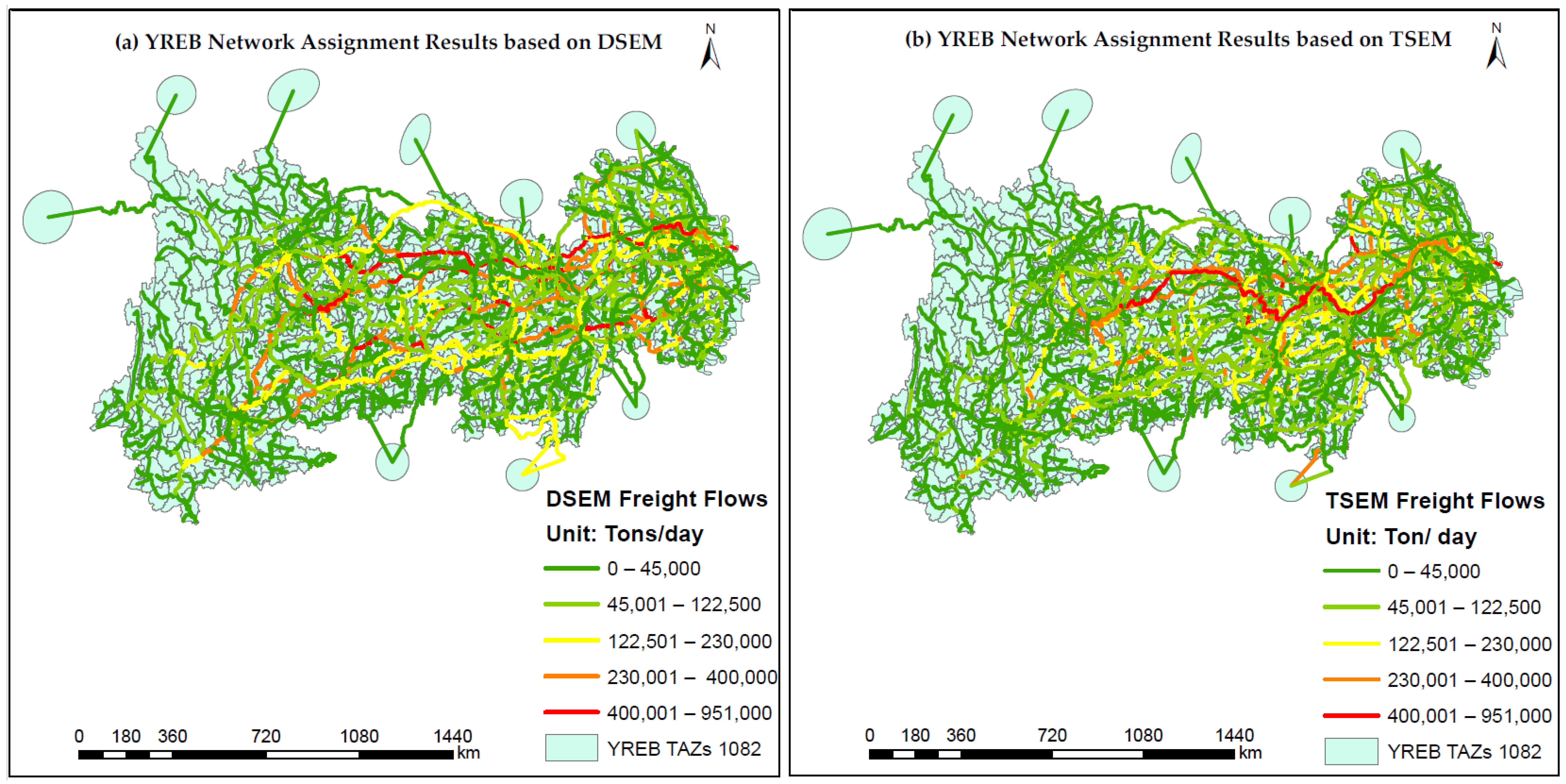
4.7. Results of Multimodal Freight Assignment Model

As outlined in Section 2.6, the multimodal freight assignment model aims to assign the forecasted OD flows of commodities obtained from the DSAA method to the multimodal supernetwork of the YREB (highway, railway, and waterway), as shown in Figure 18a, which was developed using ESRI ArcGIS 10.8 and Cube Voyage software (Version 6.5.1) (https://www.bentley.com/software/openpaths, accessed on 28 June 2024). The generalized cost function for each transportation link was specified and calibrated by incorporating four key attributes: loading costs, transfer costs, mode-specific constants, and value-per-ton considerations [12,57]. These elements were integrated into the model to reflect the actual economic and operational costs associated with freight transportation. After developing the supernetwork, the forecasted freight flows for different commodities were assigned across highway, railway, and waterway networks by using a probit-based stochastic user equilibrium method. The probit model assumes that the perceived composite cost on each link follows a multivariate normal distribution, capturing the correlations between the perceived composite travel costs on different links and provides a more behaviorally realistic framework by relaxing the restrictive IIA assumption [57]. This approach allows for a more accurate representation of freight operators’ decision-making by incorporating the uncertainty and variability associated with travel times, congestion levels, and other stochastic factors inherent in large-scale freight networks. The model was validated by comparing the estimated freight volumes on specific links with the observed annual average daily traffic (AADT) of highway links, railway station data, and port throughput data of the observed data. The results showed R² values of 0.951 for highways, 0.855 for railways, and 0.985 for waterways, demonstrating the model’s highly predictive performance for freight volumes on specific links (Figure 19 and

Table 3. Model performance comparison across transportation modes (R² Values).

Methods	Highway	Railway	Waterway
DSEM	0.951	0.855	0.985
TSEM	0.879	0.819	0.91

).

Further comparison was performed between the results of TSEM, which also assigns freight volumes between each OD pair within a multimodal transportation supernetwork (Figure 18b). The freight volumes estimated by mode in TSEM were calibrated against the observed data, including the annual average daily traffic (AADT) of highway links, railway station data, and port throughput data. The results showed that the R² values for ASEM were 0.879, 0.819, and 0.91 for highways, railways, and waterways, respectively (Figure 20) and Table 3. These results clearly demonstrate that the analytics of the proposed DSEM framework outperform its counterparts. Moreover, the proposed DSEM framework largely outperformed the TSEM previously applied to the YREB region [27]. The model developed using the proposed method provides a more objective and accurate representation of freight flows by mode and specific links, making it a valuable tool for multimodal freight transportation network analysis.

5. Conclusions and Discussion

This study proposes a DSEM method, which is an extension of the existing spatial economic modeling framework, PECAS. The proposed method first develops AEF tables and forecasts the totals of socioeconomic and demographic activities for each independent planning unit (IPU; e.g., province or city). Each IPU is responsible for creating its own plans, and has unique economic, demographic, natural, geographic, and technological features. The next step involves conducting statistical tests to identify variations in technology patterns across various sectors within the planning units considered within a region. This was followed by K-means clustering to group sectors and IPU based on similar TCs. This process allows for the development of activity totals by sector and an AEF table for defined groups. The activity totals of these groups are spatially allocated to the “nested” traffic analysis zones of each group independently using the DSAA method within the proposed DSEM framework. The spatial OD demand obtained from the DSAA was distributed across the transportation supernetwork (consisting of highways, railways, and waterways) using a probit-based stochastic user equilibrium assignment model. The proposed method was tested and validated using a case study conducted in YREB, China.

This study makes a significant methodological contribution to the advancement of SEMs by explicitly addressing regional and sectoral heterogeneity—a critical limitation of traditional large-scale SEMs. Unlike TSEM approaches that rely on the assumption of homogeneous technology patterns across large regions (e.g., YREB) without considering spatial constraints, the DSEM captures the heterogeneity in production technologies and explicitly distributes ‎economic activities to specific IPUs in the YREB. The proposed DSEM approach provides a more realistic basis for ‎region-specific planning and industrial upgrading strategies‎. The following important conclusions and policy recommendations can be drawn from the findings of this study:‎

• The calibration results for the proposed DSEM showed that the R² values between the observed and estimated link flows were 0.951, 0.855, and 0.985 for the highways, railways, and waterways, respectively. Further comparisons were performed using the traditional aggregate SEM for freight assignment results. The R² values between the observed and estimated link flows from TSEM were 0.879, 0.819, and 0.91 for the above modes. These results clearly demonstrate that the analytics of the proposed DSEM framework outperform its counterparts, indirectly confirming the model’s efficacy in predicting freight OD demand by mode and specific links.
• The Gini coefficient analysis highlights significant changes and sectoral variability in petroleum ‎processing, coal mining, and non-metal mineral extraction, where high Gini values indicate ongoing ‎transformations in TCs. Conversely, the agriculture, local services, and industrial operations sectors exhibit ‎stable TCs, suggesting sectoral resilience despite broader economic shifts. These findings ‎underscore the evolving technology patterns of the YREB, where certain industries undergo major ‎restructuring, while others maintain structural continuity over time. This analysis underscores the inadequacy of TSEM’s averaged/aggregated TCs and validates DSEM’s capability to track both structural resilience and transformation.
• The EDF forecast analysis reveals substantial inter-regional differences in the distribution of economic activities within the YREB. While aggregated forecasts suggest cumulative growth in these activities, they mask the complete absence of some activities in individual provinces—such as coal mining in Shanghai or petroleum extraction in Jiangxi, Hunan, and others. These discrepancies highlight a critical limitation of relying on regional aggregates, which can result in misleading over- or underestimations of future growth. In contrast, a disaggregated, IPU analysis offers a more objective and accurate depiction of economic development growths. This corroborates the study’s main assumption: economic activity growth is shaped by localized regional characteristics—including demographic, cultural, geographical, and technological factors. Therefore, the findings strongly advocate for differentiated, region-specific planning and policy strategies to ensure realistic and effective industrial development across diverse economic zones.
• The DSAA analysis focuses on the redistribution of economic activities across regions due to differences in technological patterns. This analysis is crucial for understanding how regional specialization evolves over time and the impact of technological advancement on spatial distribution. TSEM, which assumes that all regions operate under homogeneous economic conditions, fails to capture the complexities of regional technological development and its spatial impacts. In contrast, the DSAA method allows for the simulation of spatial shifts in economic activities, offering policymakers a more realistic understanding of how technology can reshape regional economies. The results demonstrate that DSAA provides more accurate predictions, particularly in regions with marked technological and industrial differences. The use of region-specific technology coefficients in DSEM allows for a more precise representation of technological disparities, addressing the limitations of TSEM, such as PECAS and MEPLAN, which have been criticized for their reliance on averaged/aggregated TCs [27].
• Moreover, the DSEM results on land and space utilization indicate that accounting for regional disparities is critical for managing internal migration and preventing the over-concentration of population and economic activities in major urban centers such as Shanghai, Jiangsu, and Zhejiang. The findings suggest that spatially disaggregated economic planning can play a significant role in mitigating resource scarcity and infrastructure stress in rapidly urbanizing regions, while simultaneously supporting the development of underperforming or less-industrialized areas.
• From a transportation and infrastructure perspective, policymakers should prioritize the development of multimodal transport networks that align with projected shifts in industrial activity, taking into account the spatial configuration of production, consumption, and interregional trade. Such coordination between economic forecasts and infrastructure development can significantly enhance the efficiency and equity of transport investments. The model further demonstrates that dynamic land use and economic forecasting tools like DSEM can support adaptive planning under conditions of technological change and economic transition. As regions adopt new technologies and shift their industrial base, land and resource demands evolve accordingly. Ultimately, the results demonstrate that DSEM-based forecasts provide policymakers with a more rational foundation for implementing spatially targeted economic policies, infrastructure investments, and sustainable regional development strategies.
• The findings of this study offer several practical implications for regional economic planning, industrial policies, and sustainable development. Policymakers are encouraged to account for the unique technological structure and industrial composition of each province when designing policy interventions, thereby avoiding one-size-fits-all approaches that may exacerbate regional inequalities. These findings support the assumption that economic activities in the YREB are region-specific, driven by factors like geography, infrastructure, and industrial policies. A balanced regional development strategy, focusing on investment in underdeveloped provinces such as Yunnan and Guizhou, could enhance the overall economic stability and connectivity within the YREB. Furthermore, the findings highlight that relocating labor-intensive and high-emission industries from Shanghai and Zhejiang to Yunnan, Guizhou, and Sichuan could help achieve a spatially balanced industrial development.

Limitations and Future Directions

The DSEM framework provides a scientifically robust, behaviorally consistent, and computationally adaptable decision-support system for policymakers, regional planners, and economists, making it applicable for global use by practitioners. By enabling a comprehensive examination of the dynamic interactions between real estate, production, labor, and transport markets, this study offers a foundational tool for sustainable regional planning and infrastructure investment evaluation.

Although the presents study is grounded in the spatial and sectoral context of the YREB, the DSEM framework is designed to be both generalizable and adaptable. Its core modeling principles—particularly the integration of regional technological heterogeneity and sectoral composition—can be extended to other geographic regions exhibiting similar economic characteristics. By calibrating model parameters to reflect region-specific conditions, the DSEM framework can be customized for application across both developed and developing economies. Its scalability enhances its potential utility in addressing critical policy challenges, including industrial relocation, infrastructure prioritization, and regional economic integration.

However, the empirical application of DSEM is contingent upon the availability of high-quality, region-specific datasets. The availability of regional-level economic, land use, and transportation data varies significantly across countries, further complicating the generalization of models such as DSEM. In developed economies, such as the United States and European nations, comprehensive datasets are readily available for spatial economic modeling, including national input–output tables, detailed transportation flow data, and high-resolution land use records. However, such standardized datasets are often scarce or incomplete in developing countries, making direct data acquisition challenging. To address these limitations, alternative data sources, such as government IO tables for economic activities, big data analytics on vehicle load patterns for transportation flows, and remote sensing data for spatial development, must be leveraged.

Overall, this study focuses on methodological modeling. Owing to the lack of detailed economic, land, and transport statistical data at the regional level, case studies applying the model primarily rely on available data for transportation modes, such as highway AADT, railway station data, and port throughput, to calibrate the DSEM model. In China, the national accounting economic IO table has been released every five years since 1987. However, for confidentiality reasons, the 2022 IO table has not been released yet. Consequently, this study uses the latest available IO tables from 2017. Future research should focus on collecting more comprehensive data to address the functionalities that could not be implemented in the model due to data limitations. This further enhances the effectiveness and completeness of the modeling methods proposed in this study.

References

1. Cao, X.; Ding, C.; Yang, J. Urban Transport and Land Use Planning: A Synthesis of Global Knowledge; Elsevier B.V.: Amsterdam, The Netherlands, 2022. [Google Scholar]
2. Bardal, K.G.; Reinar, M.B.; Lundberg, A.K.; Bjørkan, M. Factors facilitating the implementation of the sustainable development goals in regional and local planning—Experiences from Norway. Sustainability 2021, 13, 4282. [Google Scholar] [CrossRef]
3. Zhang, H.; Zhu, C.; Jiao, T.; Luo, K.; Ma, X.; Wang, M. Analysis of the Trends and Driving Factors of Cultivated Land Utilization Efficiency in Henan Province from 2000 to 2020. Land 2024, 13, 2109. [Google Scholar] [CrossRef]
4. Luo, Q.; Zhao, C.; Luo, G.; Li, C.; Ran, C.; Zhang, S.; Xiong, L.; Liao, J.; Du, C.; Li, Z.; et al. Rural depopulation has reshaped the plant diversity distribution pattern in China. Resour. Conserv. Recycl. 2025, 215, 108054. [Google Scholar] [CrossRef]
5. Zondag, B.; De Jong, G. The development of the TIGRIS XL model: A bottom-up approach to transport, land-use, and the economy. Res. Transp. Econ. 2011, 31, 55–62. [Google Scholar] [CrossRef]
6. Donnelly, R.; Moeckel, R. Statewide and Megaregional Travel Forecasting Models: Freight and Passenger; National Academies of Sciences, Engineering, and Medicine, Transportation Research Board; NCHRP Synthesis Report; The National Academies Press: Washington, DC, USA, 2017; Available online: https://nap.nationalacademies.org/catalog/24927/statewide-and-megaregional-travel-forecasting-models-freight-and-passenger (accessed on 10 July 2024).
7. Hensher, D.; Figliozzi, M.A. Behavioural insights into the modelling of freight transportation and distribution systems. Transp. Res.–Part B Methodol. 2007, 41, 921–923. [Google Scholar] [CrossRef]
8. Moeckel, R. Integrated Transportation and Land Use Models. National Academies of Sciences, Engineering, and Medicine. 2018. Available online: https://nap.nationalacademies.org/catalog/25194/integrated-transportation-and-land-use-models (accessed on 11 July 2024).
9. Zhong, M.; Hunt, J.D.; Abraham, J.E.; Wang, W.; Zhang, Y.; Wang, R. Advances in integrated land use transport modeling. Adv. Transp. Policy Plan. 2022, 9, 201–230. [Google Scholar]
10. Wegener, M. Land-use transport interaction models. Handb. Reg. Sci. 2021, 229, 229–246. [Google Scholar]
11. Gachanja, J.N. Towards Integrated Land Use and Transport Modelling: Evaluating Accuracy of the Four Step Transport Model—The Case of Istanbul, Turkey. Master’s Thesis, International Institute for Geo-Information Science and Earth Observation, Enschede, The Netherlands, 2010. Available online: https://essay.utwente.nl/90760/ (accessed on 31 March 2025).
12. Deng, G.; Zhong, M.; Raza, A.; Hunt, J.D.; Wang, Z. Design and development of a regional, multi-commodity, multimodal freight transport model based on an integrated modeling framework: Case study of the Yangtze River Economic Belt. In Proceedings of the Transportation Research Board 101st Annual Meeting, Washington, DC, USA, 9–13 January 2022; Available online: https://trid.trb.org/View/1900892 (accessed on 3 March 2024).
13. Thomas, I.; Jones, J.; Caruso, G.; Gerber, P. City delineation in European applications of LUTI models: Review and tests. Transp. Rev. 2018, 38, 6–32. [Google Scholar] [CrossRef]
14. Hunt, J.D.; Kriger, D.S.; Miller, E.J. Current operational urban land-use–transport modelling frameworks: A review. Transp. Rev. 2005, 25, 329–376. [Google Scholar] [CrossRef]
15. Acheampong, R.A.; Silva, E.A. Land use–transport interaction modeling: A review of the literature and future research directions. J. Transp. Land Use 2015, 8, 11–38. [Google Scholar] [CrossRef]
16. Waddell, P. Urbansim: Modeling urban development for land use, transportation, and environmental planning. J. Am. Plan. Assoc. 2002, 68, 297–314. [Google Scholar] [CrossRef]
17. Lee, J. Reflecting on an Integrated Approach for Transport and Spatial Planning as a Pathway to Sustainable Urbanization. Sustainability 2020, 12, 10218. [Google Scholar] [CrossRef]
18. Moeckel, R.; Garcia, C.L.; Chou, A.T.M.; Okrah, M.B. Trends in integrated land-use/transport modeling. J. Transp. Land Use 2018, 11, 463–476. [Google Scholar] [CrossRef]
19. Southworth, F. A Technical Review of Urban Land Use—Transportation Models as Tools for Evaluating Vehicle Travel Reduction Strategies; Oak Ridge National Laboratory, The United States Department Energy: Washington, DC, USA, 1995. [Google Scholar] [CrossRef]
20. Wegener, M. Overview of Land Use Transport Models; Emerald Group Publishing Limited: Bingley, UK, 2004; Volume 5, pp. 127–146. [Google Scholar]
21. Iacono, M.; Levinson, D.; El-Geneidy, A. Models of transportation and land use change: A guide to the territory. J. Plan. Lit. 2008, 22, 323–340. [Google Scholar] [CrossRef]
22. Batty, M. Progress, success, and failure in urban modelling. Environ. Plan. 1979, 11, 863–878. [Google Scholar] [CrossRef]
23. McFadden, D. Modelling the choice of residential location. In Cowles Foundation Discussion Papers No. 477; Yale University: New Haven, CT, USA, 1997; Available online: https://elischolar.library.yale.edu/cowles-discussion-paper-series/710/ (accessed on 13 March 2025).
24. Alonso, W. Location and Land Use: Toward a General Theory of Land Rent; Harvard University Press: Cambridge, MA, USA, 1964. [Google Scholar]
25. Leontief, W.W. Quantitative input and output relations in the economic systems of the United States. Rev. Econ. Stat. 1936, 18, 105–125. [Google Scholar] [CrossRef]
26. Fuenmayor Molero, G.J. Building a Spatial Economic Model for Caracas Using PECAS. Ph.D. Dissertation, Department of Civil Engineering, University of Calgary, Calgary, AB, Canada, 2016. [Google Scholar]
27. Deng, G.; Zhong, M.; Raza, A.; Hunt, J.D. A methodological study of multimodal freight transportation models for large regions based on an integrated modelling framework. J. Transp. Syst. Eng. Inf. Technol. 2022, 22, 30–42. [Google Scholar]
28. Wang, Z.; Zhong, M.; Pan, X. Optimizing multi-period freight networks through industrial relocation: A land-use transport interaction modeling approach. Transp. Policy 2024, 158, 112–124. [Google Scholar] [CrossRef]
29. Donnelly, R.; Upton, W.J.; Knudson, B. Oregon’s transportation and land use model integration program. J. Transp. Land Use 2018, 11, 19–30. [Google Scholar] [CrossRef]
30. Safdar, M.; Zhong, M.; Ren, Z.; Hunt, J.D. An Integrated Framework for Estimating Origins and Destinations of Multimodal Multi-Commodity Import and Export Flows Using Multisource Data. Systems 2024, 12, 406. [Google Scholar] [CrossRef]
31. Golias, M.; Mishra, S.; Psarros, I. A Guidebook for Best Practices on Integrated Land Use and Travel Demand Modeling; University of Memphis: Memphis, TN, USA, 2014. [Google Scholar]
32. Miller, R.E.; Blair, P.D. Input-Output Analysis: Foundations and Extensions; Cambridge University Press: Cambridge, UK, 2009. [Google Scholar]
33. Hunt, J.D.; Abraham, J.E. PECAS—For Spatial Economic Modelling Theoretical Formulation System Documentation. Available online: https://www.hbaspecto.com/resources/PECAS-Software-User-Guide.pdf (accessed on 30 March 2024).
34. Liu, X.; Zhou, X. Determinants of carbon emissions from road transportation in China: An extended input-output framework with production-theoretical approach. Energy 2025, 316, 134493. [Google Scholar] [CrossRef]
35. Mascaretti, A.; Dell’Agostino, L.; Arena, M.; Flori, A.; Menafoglio, A.; Vantini, S. Heterogeneity of technological structures between EU countries: An application of complex systems methods to input–output tables. Expert Syst. Appl. 2022, 206, 117875. [Google Scholar] [CrossRef]
36. Antille, G.; Fontela, E.; Guillet, S. Changes in technical coefficients: The experience with Swiss I/O tables. In Proceedings of the 13th International Conference on Input-Output Techniques, Macerat, Italy, 21–25 August 2000. [Google Scholar]
37. Ikotun, A.M.; Ezugwu, A.E.; Abualigah, L.; Abuhaija, B.; Heming, J. K-means clustering algorithms: A comprehensive review, variants analysis, and advances in the era of big data. Inf. Sci. 2023, 622, 178–210. [Google Scholar] [CrossRef]
38. Yang, X.; Zhao, W.; Xu, Y.; Wang, C.-D.; Li, B.; Nie, F. Sparse K-means clustering algorithm with anchor graph regularization. Inf. Sci. 2024, 667, 120504. [Google Scholar] [CrossRef]
39. Hennig, C.; Liao, T.F. How to find an appropriate clustering for mixed-type variables with application to socio-economic stratification. J. R. Stat. Soc. Ser. C Appl. Stat. 2013, 62, 309–369. [Google Scholar] [CrossRef]
40. Na, S.; Xumin, L.; Yong, G. Research on k-means clustering algorithm: An improved k-means clustering algorithm. In Proceedings of the 2010 Third International Symposium on Intelligent Information Technology and Security Informatics, Jinggangshan, China, 2–4 April 2010; IEEE: New York, NY, USA, 2010; pp. 63–67. [Google Scholar]
41. Doni, A.F.; Negera, Y.D.P.; Maria, O.A.H. K-means clustering algorithm for determination of clustering of Bangkalan regional development potential. In Proceedings of the IOP Conference Series, Earth and Environmental Science, Malang, Indonesia, 21–22 October 2020; IOP Publishing: Bristol, UK, 2020; Volume 485, p. 022078. [Google Scholar]
42. Çağlar, M.; Gürler, C. Sustainable Development Goals: A cluster analysis of worldwide countries. Environ. Dev. Sustain. 2022, 24, 8593–8624. [Google Scholar] [CrossRef]
43. Kumari, R.; Raman, R. Regional disparities in healthcare services in Uttar Pradesh, India: A principal component analysis. GeoJournal 2022, 87, 5027–5050. [Google Scholar] [CrossRef]
44. Azarafza, M.; Azarafza, M.; Akgün, H. Clustering method for spread pattern analysis of coronavirus (COVID-19) infection in Iran. medRxiv 2020. [Google Scholar] [CrossRef]
45. Kallingal, F.R.; Firoz, M.C. Regional disparities in social development: A case of selected districts in Kerala India. GeoJournal 2023, 88, 161–188. [Google Scholar] [CrossRef]
46. Liu, D.; Liang, J.; Xu, S.; Ye, M. Analysis of Carbon Emissions Embodied in the Provincial Trade of China Based on an Input–Output Model and k-Means Algorithm. Sustainability 2023, 15, 9196. [Google Scholar] [CrossRef]
47. Yuan, C.; Yang, H. Research on K-Value Selection Method of K-Means Clustering Algorithm. J 2019, 2, 226–235. [Google Scholar] [CrossRef]
48. Thorndike, R.L. Who belongs in the family? Psychometrika 1953, 18, 267–276. [Google Scholar] [CrossRef]
49. Wang, J.; Biljecki, F. Unsupervised machine learning in urban studies: A systematic review of applications. Cities 2022, 129, 103925. [Google Scholar] [CrossRef]
50. Den Teuling, N.G.P.; Pauws, S.C.; van den Heuvel, E.R. A comparison of methods for clustering longitudinal data with slowly changing trends. Commun. Stat.-Simul. Comput. 2023, 52, 621–648. [Google Scholar] [CrossRef]
51. Liu, Y. Modelling Urban Development with Geographical Information Systems and Cellular Automata; CRC Press: Boca Raton, FL, USA, 2008. [Google Scholar]
52. Petropoulos, F.; Apiletti, D.; Assimakopoulos, V.; Babai, M.Z.; Barrow, D.K.; Taieb, S.B.; Bergmeir, C.; Bessa, R.J.; Bijak, J.; Boylan, J.E. Forecasting: Theory and practice. Int. J. Forecast. 2022, 38, 705–871. [Google Scholar]
53. HBA Specto Incorporated Production, Exchange, and Consumption Allocation System (PECAS). Available online: https://www.hbaspecto.com/ (accessed on 23 March 2024).
54. Mir, M.S.; Rao, K.V.K.; Hunt, J.D. Space development modeling of urban regions in developing countries. J. Urban Plan. Dev. 2010, 136, 75–85. [Google Scholar] [CrossRef]
55. Wang, W.; Zhong, M.; Zhang, Y.; Li, Y.; Ma, X.; Hunt, J.D.; Abraham, J.E. Testing microsimulation uncertainty of the parcel-based space development module of the Baltimore PECAS Demo Model. J. Transp. Land Use 2020, 13, 93–112. [Google Scholar] [CrossRef]
56. Yamada, T.; Imai, K.; Nakamura, T.; Taniguchi, E. A supply chain-transport supernetwork equilibrium model with the behaviour of freight carriers. Transp. Res. Part E Logist. Transp. Rev. 2011, 47, 887–907. [Google Scholar] [CrossRef]
57. Dios Ortúzar, J.d.; Willumsen, L.G. Modelling Transport; Wiley: Hoboken, NJ, USA, 2011. [Google Scholar]
58. Sebastian, I.; Li, J. Outline for Building China’s Strength in Transport; Deutsche Gesellschaft für Internationale Zusammenarbeit (GIZ) GmbH: Bonn and Eschborn, Germany, 2019; Available online: https://changing-transport.org/wp-content/uploads/2019_Outline_for_Building_Chinas_Strength_in_Transport.pdf (accessed on 12 March 2025).
59. National Bureau of Statistics of China. In Obtenido de National Bureau of Statistics of China. 2016. Available online: https://www.stats.gov.cn/english/ (accessed on 13 March 2024).
60. OpenStreetMap. OpenStreetMap Foundation. 2024. Available online: https://www.openstreetmap.org (accessed on 30 March 2024).
61. Esri. ArcGIS Online. Esri 2024. Available online: https://www.arcgis.com (accessed on 30 March 2024).
62. Department of National Economic Accounting, State Statistical Bureau of P.R. China. China Regional Input-Output Table 2007; China Statistical Publishing House: Beijing, China, 2007. [Google Scholar]
63. Department of National Economic Accounting, State Statistical Bureau of P.R. China. China Regional Input-Output Table 2012; China Statistical Publishing House: Beijing, China, 2016. [Google Scholar]
64. Department of National Economic Accounting, State Statistical Bureau of P.R. China. China Regional Input-Output Table 2017; China Statistical Publishing House: Beijing, China, 2020. [Google Scholar]
65. Ren, Z.; Zhong, M.; Cui, G.; Li, L.; Zhao, H. An Iterative Method for Calibrating Freight Value-per-Ton Conversion Factors of Integrated Land Use Transport Models Based on Multi-Source Data. In Proceedings of the Transportation Research Board 103rd Annual Meeting, Washington, DC, USA, 7–11 January 2024; Available online: https://trid.trb.org/View/2317332 (accessed on 13 March 2025).
66. Research and Markets, China Construction Market, Trends and Forecast Analysis to 2028-Construction Industry Set to Record an Average Annual Growth Rate of 3.9% Between 2025 and 2028. 2024. Available online: https://www.businesswire.com/news/home/20241111813514/en/China-Construction-Market-Trends-and-Forecast-Analysis-to-2028---Construction-Industry-Set-to-Record-an-Average-Annual-Growth-Rate-of-3.9-between-2025-and-2028---ResearchAndMarkets.com (accessed on 29 March 2025).
67. GlobalData. China Construction Market Size, Trend Analysis by Sector, Competitive Landscape and Forecast to 2028-Q4 Update. 2025. Available online: https://www.globaldata.com/store/report/china-construction-market-analysis/ (accessed on 31 March 2025).
68. Xu, H.; Hu, S.; Li, X. Urban Distribution and Evolution of the Yangtze River Economic Belt from the Perspectives of Urban Area and Night-Time Light. Land 2023, 12, 321. [Google Scholar] [CrossRef]
69. Zheng, H.; Bai, Y.; Wei, W.; Meng, J.; Zhang, Z.; Song, M.; Guan, D. Chinese provincial multi-regional input-output database for 2012, 2015, and 2017. Sci. Data 2021, 8, 244. [Google Scholar] [CrossRef]
70. Brakman, S.; Garretsen, H.; Van Marrewijk, C. An Introduction to Geographical Economics: Trade, Location and Growth; Cambridge University Press: Cambridge, UK, 2001. [Google Scholar]
71. Fujita, M.; Krugman, P.R.; Venables, A. The Spatial Economy: Cities, Regions, and International Trade; MIT Press: Cambridge, MA, USA, 2001. [Google Scholar]
72. Zondag, B. Joint Modeling of Land-Use, Transport and Economy. Ph.D. Thesis, Delft University of Technology, Delft, The Netherlands, 2007. [Google Scholar]
Figure 1. A schematic diagram of the proposed differential spatial economic modeling method.
Land 14 00886 g001
Figure 2. Analytical framework for identifying regional technology pattern disparity.
Land 14 00886 g002
Figure 3. Aggregate space development growth curve.
Land 14 00886 g003
Figure 4. Study area: Yangtze River Economic Belt, China.
Land 14 00886 g004
Figure 5. Trend of GDP per capita (RMB/person) in the regions of the YREB.
Land 14 00886 g005
Figure 6. (a) YREB traffic analysis zones; (b) multimodal transportation network of the YREB.
Land 14 00886 g006
Figure 7. Technical coefficients of each province of YREB and aggregate YREB.
Land 14 00886 g007aLand 14 00886 g007b
Figure 8. Results of Gini index for technical coefficients between 2007 and 2012.
Land 14 00886 g008aLand 14 00886 g008b
Figure 9. Results of K-means clustering for coal mining and processing activity: (a) elbow method for optimal clusters; (b) Cluster 1; (c) Cluster 2; (d) Cluster 3; (e) Cluster 4.
Land 14 00886 g009
Figure 10. Results of K-means clustering for metal smelting activity: (a) elbow method for optimal clusters; (b) Cluster 1; (c) Cluster 2; (d) Cluster 3.
Land 14 00886 g010
Figure 11. Results of K-means clustering for other industrial operation activity: (a) elbow method for optimal clusters; (b) Cluster 1; (c) Cluster 2; (d) Cluster 3; (e) Cluster 4; (f) Cluster 5.
Land 14 00886 g011
Figure 12. Forecast economic and demographic activities in YREB regions from 2012 to 2050: (a) Anhui; (b) Guizhou; (c) Hubei; (d) Hunan; (e) Jiangsu; (f) Chongqing; (g) Zhejiang; (h) Yunnan; (i) Jiangxi; (j) Sichuan; (k) Shanghai; (l) YREB.
Land 14 00886 g012aLand 14 00886 g012b
Figure 13. Forecasting of household activities: (a) individual planning unit of YREB (b), aggregate YREB.
Land 14 00886 g013
Figure 14. Comparative results of smelting and processing metals products; (ac) differential spatial activity allocation in 2012; (df) differential spatial activity allocation in 2050; (g) aggregate activity allocation in 2012 and (h) in 2050.
Land 14 00886 g014
Figure 15. Comparative results of transportation and postal operations activity; (a,b) differential spatial activity allocation in 2012; (c,d) differential spatial activity allocation in 2050; (e) aggregate activity allocation in 2012 and (f) in 2050.
Land 14 00886 g015
Figure 16. Comparative results of the estimated amount of industrial space (million m2): (ac) DSEM forecast; (df) TSEM forecast.
Land 14 00886 g016
Figure 17. Comparative results of DSEM and TSEM OD flows. (a,b) Cereal; (c,d) coal.
Land 14 00886 g017
Figure 18. Comparative results of a multimodal freight assignment: (a) differential spatial economic modeling results; (b) traditional aggregate spatial economic modeling results.
Land 14 00886 g018
Figure 19. Results of freight assignment by link for three modes, using the differential spatial economic method.
Land 14 00886 g019
Figure 20. Results of freight assignment by link for three modes, using the traditional aggregate spatial economic method.
Land 14 00886 g020