Abstract
CO2 is the primary contributor to global warming, and also the most significant anthropogenic emission gas in cities. This study investigates near-surface CO2 spatiotemporal variability patterns at the community scale to address the critical gap in urban CO2 high-resolution measurement and promote urban carbon neutrality. Combining fixed and mobile monitoring across five representative communities (1-km2 coverage) with two-hour temporal precision and 20 m spatial resolution, results revealed average CO2 concentrations of 440–480 ppm, exhibiting bimodal diurnal cycles and highlighting spatiotemporal divergent emission behaviors. Three communities peaked during 17:00–19:00 LT, while two peaked during 08:00–10:00 LT. Spatial correlation analysis identified two dominant patterns: road-adjacent “externally dominated” hotspots and “internally dominated” zones with elevated intra-community levels. Spearman correlation analysis, Random Forest, and Geographically and Temporally Weighted Regression models quantified spatial morphology and element contributions, demonstrating that building morphology exerted time-varying impacts across communities. Meanwhile, external traffic contributed 18–39% to concentration variability, while internal traffic and energy consumption drove localized peaks. The findings indicated that apart from the emission sources, the micro-scale urban spatial design elements also regulate the near-surface CO2 distribution. This high-resolution approach provides actionable insights for optimizing community layouts and infrastructure to mitigate localized emissions, advancing carbon neutrality targeted urban planning.
1. Introduction
CO2 is a non-self-generating greenhouse gas that comes mainly from fossil energy consumption in human production and living processes. Additionally, the gaseous molecular properties of CO2 enable it to absorb infrared radiation, causing and exacerbating the greenhouse effect. In high-density urban environments, urban communities serve as spatial carriers of residential activities and direct CO2 emissions [1]. Prior studies have indicated that urban communities, as important sites of human activity, account for approximately 30–40% of the total anthropogenic greenhouse gases globally [2]. And this proportion exceeds 40% in China, indicating a significant potential for emission reduction [3]. Furthermore, as atmospheric CO2 concentrations rise, they lead to increased heat absorption and re-radiation, intensifying the greenhouse effect in urban areas and serving as a catalyst for extreme climatic hazards.
Understanding the spatial and temporal characteristics of near-surface CO2 concentrations in urban communities is crucial for effective in situ sequestration mitigation strategies, which are essential for achieving carbon neutrality in built environments [4,5]. Therefore, obtaining high-precision measurements of near-surface CO2 and analyzing its distribution has become a priority for identifying relevant influencing factors. In recent years, multiple measurements of urban CO2 levels worldwide have shown that urban areas exhibit a pronounced CO2 dome effect, with concentrations in high-density urban regions generally exceeding those in suburban or rural areas by 20–50 ppm [6,7]. In high-density urban environments, CO2 concentrations display relatively regular patterns. CO2 concentrations on weekdays follow a specific fluctuation pattern, peaking in the early morning and declining their lowest levels in the afternoon [8,9]. However, observations indicate notable spatial and temporal distribution differences in CO2 levels across different space types of cities and communities that do not precisely follow the “peak–valley” pattern [10,11,12]. This variability suggests that the near-surface CO2 in urban residential communities is influenced by a range of spatial factors, including anthropogenic and geogenic emissions. Therefore, investigating the spatial and temporal distribution characteristics and factors influencing near-surface CO2 emissions is vital for identifying high-concentration zones and analyzing the underlying causes of their formation.
Table 1 summarizes the measurement methods researchers have adopted to analysis the spatial and temporal characteristics of urban CO2 levels, including continuous measurement methods of both near-surface and roof of building height, and mobile measurement methods.

Table 1.
Summary of existing studies on measuring urban carbon concentrations.
- The continuous measurement method relies on CO2 concentration data collection at common or multiple points [22], which is unable to assess the distribution of CO2 at a high spatial resolution because of the sparsity of fixed measurement points [23].
- The mobile measurement allows for the study of highly fine-grained CO2 spatial distribution characteristics, yielding reliable, reproducible, and representative results [21]. A comparison of urban canopy cross sections and near-surface CO2 monitoring results indicated that urban CO2 emissions mainly stem from near-surface human activities [24], and the moving measurement is more adaptable for identifying the sources of CO2 at a height of 1–3 m above the ground [25].
However, the limitations of the measurement methods in the existing studies result in CO2 measurement outcomes that cannot simultaneously achieve high temporal and spatial resolutions. Therefore, current research lacks attention to near-surface CO2 distribution at the neighborhood scale, making it difficult to resolve the influence of spatial elements on near-surface CO2 levels.
This study aims to explore the spatial and temporal variability of near-surface CO2 in typical urban communities and the impact of urban spatial factors on near-surface CO2. The three main focused research questions are as follows:
RQ1: how can high-temporal and spatial-resolution near-surface CO2 measurements be conducted in urban communities?
RQ2: what are the spatiotemporal characteristics of near-surface CO2 concentrations in representative urban communities?
RQ3: which spatial factors impact on the variability of near-surface CO2 in urban communities?
2. Materials and Methods
2.1. The Framework of the Study
The measurement and analysis of near-surface CO2 spatial and temporal variability for different types of communities will follow a five-part logic that includes the selection of representative community samples, the near-surface CO2 concentration measurements, the spatial and temporal characterization evaluations, and spatial influencing factor analyses (Figure 1). Step 1 establishes representative sampling through morphological clustering analysis of urban form parameters, including building geometry, morphology, density, and layout. Five distinct community types were systematically selected using machine learning-assisted categorization.
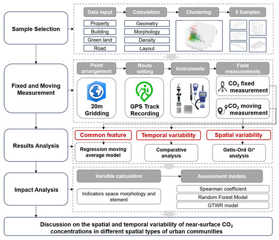
Figure 1.
Technical framework of the study.
Step 2 implements a dual-mode measurement protocol combining fixed-point and mobile monitoring. High-precision CO2 sensors were deployed in a 20 × 20 m grid configuration, synchronized with GPS-tracked mobile measurements along predefined routes. Continuous data collection spanned 24 h periods to capture diurnal variations.
Step 3 incorporates multi-scale analytical techniques: (1) temporal trends were decomposed using Regression Moving Average (RMA) modeling; and (2) spatial heterogeneity was quantified through Getis-Ord Gi* hotspot analysis.
Step 4 evaluates driving mechanisms through Spearman’s rank correlation, Random Forest feature importance ranking (500 trees, R2 = 0.82, RMSE = 0.18), and Geographically and Temporally Weighted Regression (GTWR) with adaptive bandwidths.
Step 5 synthesizes findings through comparative analysis across neighborhood typologies, establishing mechanistic links between urban morphology and CO2 dispersion patterns. This hierarchical framework enables systematic integration of urban form data, microenvironmental monitoring, and spatiotemporal modeling, addressing critical challenges in urban carbon emission characterization.
2.2. Sample Selection
Based on the research content, Nanjing, which is characterized by a typical high-density urban environment, was chosen as the sample for the study. Nanjing is located in an economically developed region of the Yangtze River Delta in China, and is a typical Chinese megacity. This study focuses on the central area of Nanjing city (latitude 32°3′41.6″ N, longitude 118°47′29.6″ E), which is the core region of this important eastern Chinese city. This area is characterized by a high population density, high spatial density, and frequent economic activities, exhibiting typical features of a high-density urban environment and encompassing various typical urban residential types found globally.
To select the spatial scope of the research samples, we first employed the k-means unsupervised clustering method to classify the indicators of urban communities. Five typical spatial types of urban communities were identified (see Table 2 for space morphology indicators and their calculation formulas, and Appendix A shows details about data acquisition, clustering methods, and results).
Table 2.
Space morphology indicators for the classification of high-density urban communities.
Subsequently, to ensure the validity of the CO2 measured results, five adjacent urban communities in the central area of Nanjing city were selected as the research samples (Figure 2). These samples represented typical community types, with inter-sample distances not exceeding 1 km. Previous studies have indicated that selecting samples within this range allows for the investigation of the spatial and temporal variability of near-surface CO2 distribution and its influencing factors, while controlling for external factors such as urban traffic flow, population density, and urban microclimate [26].
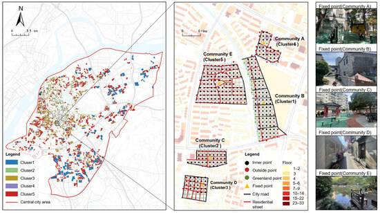
Figure 2.
Urban community clustering results, location of measurement points in samples, and photographs of fixed measuring points.
Five selected urban communities exhibited typical spatial characteristics (Table 3). Community A (Cluster1, 6.52%) was characterized as a high-rise apartment with a high plot ratio. Community B (Cluster2, 6.42%) represented villa communities, which are characterized by large areas, consisting of low-rise (2–4 stories) detached houses. Community C (Cluster 3, 46.16%) was identified as row houses built during 1980s–2000s, which are the most common type in Chinese cities [27], and characterized by medium heights (7–13 stories). Community D (Cluster 4, 19.54%) is mainly distributed within the old city, and represents typical urban village communities, which are characterized by small plot sizes, low plot ratios, and extremely high building coverages, predominantly consisting of single-story bungalow [28]. Community E belongs to Cluster 5 (21.35%) and is a newly built residential district, which is characterized by a large plot size, relatively high average height (16–30 stories), and high open space ratio.
Table 3.
Spatial information of community samples.
2.3. CO2 Measurement Scheme
The measurement scheme consisted of three phases (Figure 3). From 14 to 16 May 2024, measurements were conducted on five samples, including two days of common weather (average wind speed: 1.9 m/s; maximum wind speed: 3.3 m/s), and one day of windy weather (average wind speed: 2.9 m/s; maximum wind speed: 7.5 m/s). The selection of these measurement days was based on their ability to represent common carbon emission conditions observed on working days throughout the year. Furthermore, during the spring season (April to June), near-surface atmospheric turbulence remains relatively stable, and near-surface CO2 concentrations are less influenced by non-spatial climatic factors. This makes it more suitable to reflect the impact of community spatial configurations on CO2 concentrations [29,30].
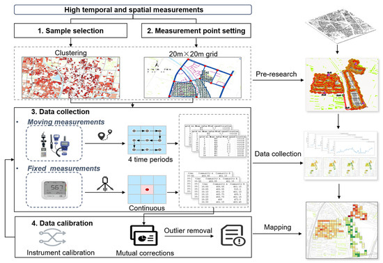
Figure 3.
Measurement flowchart.
A combination of fixed and mobile measurement methods was employed, collect two sets of measured data that complement and verify each other, which allowed high temporal and spatial precision. This approach provides better adaptability for measuring CO2 at heights of approximately 1–3 m above the ground, which effectively represents atmospheric conditions at this scale, and helps avoid potential turbulence and obstacles near the ground [21].
To ensure the reliability and validity of the CO2 measurement scheme, we implemented a systematic approach to the selection of both mobile measurement routes and fixed measurement points. The selection process was guided by several key criteria: Firstly, the measurement points were chosen to capture the diversity of spatial features within each urban community. We ensured that the selected points represented various land use types, such as residential, commercial, and green spaces, to provide a comprehensive assessment of CO2 distribution. Secondly, the routes for mobile measurements were planned to maximize accessibility. By dividing the communities into grids, we ensured adequate spatial coverage, allowing for detailed mapping of CO2 concentrations. Thirdly, to account for temporal variations in CO2 emissions, mobile measurements were conducted at four distinct time periods throughout the day, allowing to capture diurnal variations in CO2 levels. Lastly, the fixed measurement points were strategically located in open spaces at the center of each urban community.
This positioning minimized interference from surrounding structures and ensured that the measurements were representative of the broader community environment. The 24 h continuous data collection at these points provided a stable reference for validating mobile measurements.
2.4. Measuring Methods
2.4.1. Measuring Instruments
The primary measurements in this study were CO2 concentration. We used dual-wavelength non-infrared diffusion (NDIR) measuring instruments, specifically the TSI-7515 and TSI-7525 models (Table 4). These devices are characterized by high precision and stability, which ensure the validity of the measurement results [30,31,32].
Table 4.
Parameters of measurement instruments.
For fixed measurements, a non-infrared diffusion CO2 detector equipped with Wi-Fi functionality was employed, allowing continuous outdoor monitoring. The instrument was positioned at a height of 1.2 m in an open area.
To address potential discrepancies between the fixed sensor (Qingping, the equipment was sourced by Qingping Technology (Beijing) Co., Ltd., Shenzhen Branch, Shenzhen, China) and the mobile sensor (TSI-7515/7525, the equipment was sourced from TSI Inc., located in Shoreview, MN, USA), a series of calibration and consistency control measures were implemented. The main procedures included preheating and zero calibration, followed by cross-validation of the two datasets. First, the measurement instruments were zero-calibrated using high-purity nitrogen (CO2 ≈ 0 ppm), and all instruments were preheated for 10–15 min prior to each measurement session. After the measurements, the fixed-point data were spatiotemporally matched with the mobile data, and the relative deviation between the two datasets was calculated, with the mean deviation controlled within <5 ppm. Outliers exceeding 3σ were excluded from further analysis. These calibration steps effectively minimized potential discrepancies between instruments, enhancing the overall accuracy and consistency of data collected in both fixed and mobile measurement scenarios. Additionally, GPS logging software (2bulu APP V7.9.7) and spatiotemporal data-matching techniques were employed to ensure data traceability.
2.4.2. Fixed and Mobile Measurements
To investigate CO2 concentration variations in urban communities, data collection was divided into two parts: fixed measurements and mobile measurements (Figure 3 illustrates the specific workflow). The core steps are as follows:
- (1)
- Sample selection: five typical community types were selected through morphological cluster analysis.
- (2)
- Design of measurement points: Communities were divided into 20 m × 20 m grids. Points completely obstructed by buildings were excluded, resulting in the identification of 285 measurement points (29.8% of which were near roads). The grid centers were used as mobile measurement points, while fixed measurement points were located in the central open area of each community, suitable for 24 h instrument placement.
- (3)
- Data collection:
- Fixed measurements: instruments were placed at a height of 1.2 m, continuously recording CO2 concentrations for 24 h, with data collected at 10 min intervals.
- Mobile measurements: Conducted in four time periods each day (LT8–10, LT11–13, LT14–16, LT17–19) along preset routes. Each point was sampled for 30 s with the instrument, and all points were measured within approximately two hours [33].
- (4)
- Data calibration: All instruments were calibrated with standard gases prior to measurements. Cross-validation was conducted between mobile and fixed data, achieving an average measurement accuracy of 96.8%.
2.5. Data Analysis Methods
2.5.1. Space Influencing Indicators
The spatial impact indicator system comprises both spatial morphology indicators and spatial distribution indicators. Spatial morphology indicators quantify the geometric characteristics of urban communities. Based on the morphological clustering results obtained during the sample selection phase described in Section 2.2, this study selected seven representative parameters: Plot Area (PA), Plot Perimeter (PP), Building Density (BD), Far Area Ratio (FAR), Average Height (AH), and Enclosure Degree (ED), with their calculation formulas detailed in Table 2.
Spatial distribution indicators characterize the topological relationships of internal spatial elements, reflecting the interaction between human activities and natural processes. Existing research demonstrates that road networks, building layouts, and green space systems influence near-surface CO2 distribution through differentiated carbon source/sink mechanisms [34,35,36]. This study established multi-level road impact indicators:
- Distance to External Transportation (DO): shortest path from monitoring points to boundary roads of communities;
- Distance to Internal Streets (DS): Euclidean distance from monitoring points to community-level roads;
- Distance to Intersections (DI): topological distance from monitoring points to nearest road intersections.
Building impact is characterized by the Distance to Building Energy Consumption (DB), defined as the weighted distance from monitoring point centers to the nearest residential buildings (weight = building volume × occupancy rate). The green space effect was quantified through the Normalized Difference Vegetation Index (NDVI)-adjusted Green Space Ratio (GR),
where Ai represents the area of raster cells meeting vegetation coverage criteria (NDVI > 0.3), and PA denotes the total area of the community. This metric simultaneously captures both the spatial extent and ecological efficacy of green spaces, demonstrating greater biophysical significance compared to conventional area-based ratios.
2.5.2. Spearman Correlation Analysis
This study employed Spearman’s correlation coefficient as a bivariate correlation method for univariate analysis to assess the monotonic relationship between near-surface CO2 in urban communities and spatial factor variables. Compared with the Pearson correlation analysis, the Spearman correlation analysis is more suitable for evaluating nonlinear relationships between variables, and does not impose requirements on the overall distribution pattern of the sample, making it a more appropriate method for the data conditions of this study [37].
2.5.3. Random Forest Model
A Random Forest (RF) model was used to capture the complex nonlinear relationships between spatial elemental variables and CO2 concentrations in different types of urban communities to assess the contribution of each spatial elemental variable. The random forest model has demonstrated high accuracy in multiparameter predictions, and has been widely used in urban studies [38,39]. Compared with other machine learning models, the Random Forest model offers better interpretability, and can provide an intuitive understanding of the contribution of each underlying spatial element variable to the distribution of CO2 concentrations [40].
2.5.4. Geographically and Temporally Weighted Regression Model
Due to the significant spatial heterogeneity and temporal dynamics of CO2 driving factors in urban communities, traditional regression models struggle to capture these variations. The Geographically and Temporally Weighted Regression (GTWR) model addresses this limitation by integrating a temporal weighting function into the classical Geographically Weighted Regression (GWR) model [41]. The GTWR model is expressed as follows:
where denotes the spatiotemporal coordinates of observation i, represents the local regression coefficient for variable k, and is the error term. The dual bandwidth optimization process accounts for urban mobility patterns (spatial) and diurnal emission cycles (temporal), capturing the metastable nature of near-surface CO2 dispersion.
The GTWR model’s strength lies in its ability to simultaneously consider spatial and temporal effects on CO2 concentrations. For example, traffic impacts may intensify during rush hours [42], while building distributions may affect CO2 emission variations according to daytime or nighttime meteorological conditions [43]. By adaptively optimizing spatial and temporal bandwidths, the GTWR model accurately captures these dynamic relationships.
In this study, we tested Ordinary Least Squares (OLS), GWR, and GTWR models. After testing for multicollinearity, results revealed that GTWR significantly outperformed both OLS and GWR (Table 5). Using the golden section search method, GTWR’s spatial bandwidth was set to and its temporal bandwidth to . The superior performance of GTWR (R2 = 0.512, AICc = 9562) demonstrates its reliability in analyzing spatiotemporal CO2 variability in urban communities. Therefore, we used GTWR to compute and visualize the regression coefficients of five spatial variables, with 0 as the critical value to distinguish between positive and negative effects.
Table 5.
Evaluation results of the OLS, GWR, and GTWR models.
3. Results
3.1. General Characteristics
According to the measured results, near-surface CO2 concentrations in urban communities exhibited distinct common characteristics in both temporal and spatial distributions. Under typical weather conditions, the average near-surface CO2 concentration in these communities ranged from 440 to 480 ppm, which is consistent with observations in the urban communities of Shanghai [30]. In comparison, the global monthly mean CO2 concentration was 425.19 ppm in December 2024 [44], indicating that urban areas typically exhibit higher CO2 levels due to local anthropogenic emissions.
In terms of temporal distribution, as illustrated in Figure 4a, CO2 levels across the five urban communities displayed a similar bimodal pattern over a 24 h period on weekdays. This pattern was further refined using linear regression to produce a combined curve in Figure 4b. The results revealed a significant increase in the concentration during the early morning and evening hours, with an average growth rate of 0.04%, peaking at 479.55 ppm. Conversely, the concentrations declined during the noon and afternoon periods.
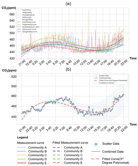
Figure 4.
Temporal distribution of CO2 in urban communities: (a) near-surface CO2 measurement curve (weekday, no wind); (b) fitted CO2 curves for five communities.
On a typical week day, near-surface CO2 concentrations in the urban communities reached their lowest point, but showed the greatest fluctuations during the LT10–15 time period, with an hourly difference of up to 8.98 ppm. This fluctuation reflects variations in the direct CO2 emission intensity in urban communities across different times. These variations align with urban mobility patterns during the daytime, as supported by statistical findings indicating that afternoon dynamic and traffic density fluctuates significantly across various urban areas [45].
Additionally, Figure 5 indicates that CO2 concentrations at measurement points within urban neighborhoods that are not adjacent to roads are generally lower than the overall average, with minor differences ranging from −0.94 ppm to 5.90 ppm. This suggests that external emission sources significantly influence CO2 levels. To facilitate a more comprehensive analysis of the temporal and spatial differentiation characteristics of near-surface CO2, this study further explored both temporal and spatial variability.
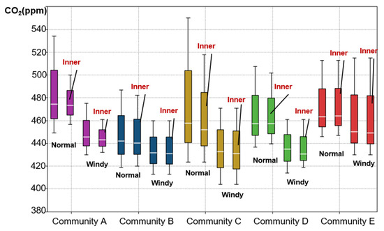
Figure 5.
Box plots of CO2 level for different communities during normal and windy weather, plotting all grids and internal grids (not adjacent to roads) separately.
3.2. Temporal Variability
The results from mobile and fixed measurements in the five sampled communities revealed significant temporal variations in CO2 levels, including distinct daily fluctuation patterns and peak characteristics across different urban communities. The mobile measurement data indicated differentiated average CO2 values and daily variation trends (Figure 6a). Community A consistently exhibited the highest near-surface CO2 levels across all four time periods, with a peak value of 485.59 ppm recorded during the LT17–19 period. In contrast, Community B maintained relatively low CO2 throughout the LT11–19 period, reaching a minimum of 426.64 ppm during the LT11–13 period. The lowest value in the LT8–10 period was found in Community D, at 447.22 ppm.

Figure 6.
Temporal differentiation characteristics of CO2 in urban communities: (a) near-surface CO2 of 4 time periods (mobile measurement). These violin plots reflect the distribution of CO2 concentrations inside (left, within the communities) and outside (right, near the roads) at different times in the five communities. The red color represents the CO2 distribution during 8:00–10:00 local time, yellow represents 11:00–13:00, green represents 14:00–16:00, and blue represents 17:00–19:00. The lines in the figure represent the daily variations of the five communities; (b) near-surface CO2 moving average curve of 24 h in five communities (fixed measurement). It can be observed that the main changes and some steep variations occur during periods of human activities, which are also the time periods covered by the mobile measurements.
Regarding daily variation patterns, Communities A, C, and D showed consistency, with the highest average CO2 levels recorded during the LT17–19 period at 485.59 ppm, 480.63 ppm and 475.78 ppm, respectively. Subsequently, CO2 levels were lower during the LT14–16 and LT8–10 periods, with the minimum levels occurring during the LT11–13 period. In contrast, Communities B and E exhibited a different pattern, with peak near-surface CO2 levels occurring during the LT8–10 period, measuring 461.86 ppm and 469.27 ppm, respectively.
The fixed measurement results illustrated the continuous distribution and variations in near-surface CO2 levels across central open spaces in the five communities, highlighting the differences in peak fluctuations (Figure 6b). Specifically, Community A exhibited higher near-surface CO2 levels, greater fluctuations, and elevated peaks during LT8–13 period, with the peak value reaching 493.3 ppm. Community C displayed abnormally high near-surface CO2 levels and significant fluctuations during the LT7–8 and LT16–22 periods, notably recording two anomalous peaks at LT11 and LT13, measuring 477.3 ppm and 502.3 ppm, respectively. Meanwhile, during the LT13–17 period, Community E experienced greater fluctuations in the near-surface CO2 levels, peaking at 470 ppm. Additionally, Community D demonstrated relatively low near-surface CO2 levels with minor fluctuations during the LT10–15 period.
Compared with the mobile measurement results, the findings from fixed measurements further indicate that the temporal differentiation of near-surface CO2 levels among different communities primarily occurs during periods of human activity (LT 7–22). Moreover, the five-minute temporal resolution of fixed measurements effectively captured short-term CO2 fluctuations induced by human activities.
3.3. Spatial Variability
Because of the limitations of fixed measurements in capturing CO2 distribution differences at various locations within communities [46], this study primarily employed mobile measurement results to analyze the spatial differentiation characteristics of near-surface CO2 in communities, while utilizing fixed measurement methods for multi-point calibration of the mobile measurement results. The results indicated that, regarding the average concentration differences in near-surface CO2 across communities (Figure 7a), Communities A and E had noticeably higher average CO2 levels compared to others, at 474.39 ppm and 463.28 ppm, respectively, whereas Community B had the lowest average concentration of 442.18 ppm. In terms of spatial differences in near-surface CO2 (Figure 7b,c), Community C showed the greatest overall concentration difference compared with its internal concentrations (5.80 ppm, 1.28%), and the difference between maximum and minimum CO2 values for Communities C was relatively large, indicating an uneven CO2 spatiotemporal distribution.
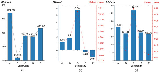
Figure 7.
Spatial differentiation characteristics of CO2 in urban communities: (a) average near-surface CO2 concentrations (ppm); (b) differences between overall grids and grids not adjacent to roads (ppm); (c) differences between maximum and minimum CO2 levels in the five communities (ppm).
Based on these results, the study further visualized the gridded CO2 concentrations spatially (Figure 8a). It was found that near-surface CO2 levels across the five communities generally exhibited two types of spatial distribution patterns (Figure 8b). The external high-concentration dominant type is characterized by higher CO2 levels along the outer edges of the communities, with lower internal CO2 levels. CO2 hotspots tend to be adjacent to external roads and intersections, such as in Communities A and C. The second spatial distribution pattern was the internal high-concentration dominant type, where high CO2 concentration areas were found internally rather than along the outer edges, as seen in Communities B, D, and E. Furthermore, fixed measurement data revealed the presence of localized anomalous hotspots in internally high-concentration dominant communities, whereas the riverside area of Community B showed significantly low concentrations, supporting the notion that water bodies serve as important factors in carbon sinks within high-density built environments [43].
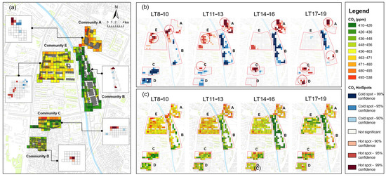
Figure 8.
Characteristics of CO2 spatial differentiation in urban communities: (a) Average CO2 concentration and hotspots in each community. It can be observed that the hotspots of Community A and C are located on the outside, while the hotspots of Community B, D, and E are located on the inside.; (b) Getis–Ord Gi* hotspot result at different time periods; (c) distribution of near-surface CO2 at different time periods.
Combined with the temporal variation analysis (Figure 8c), it was observed that during the LT 8–10 and LT 14–16 periods, CO2 concentrations along the roadsides were generally higher, with near-surface CO2 concentration peaks aligned with morning and evening traffic peaks [47,48]. Conversely, during the LT 11–13 and LT 17–19 periods, CO2 hotspots emerged within the communities, potentially indicating the impact of household energy use on near-surface CO2 levels. To further investigate the influencing factors of temporal and spatial differentiation characteristics of near-surface CO2 in communities, this study discussed the causes of these spatiotemporal differentiation characteristics from the perspectives of spatial factors influences.
4. Analysis of Spatial Influencing Factors
As specified in Section 2.5.2, this study employed six spatial morphology metrics (PP, PA, BA, FAR, AH, and ED) and five spatial distribution indicators (DO, DS, DI, DB, and GR). Three analytical approaches were integrated to investigate spatial impacts on near-surface CO2 concentrations at the community scale: Spearman’s rank correlation coefficient for nonparametric relationship detection, Random Forest (RF) machine learning for nonlinear pattern identification, and Geographically and Temporally Weighted Regression (GTWR) for spatiotemporal heterogeneity modeling.
4.1. Correlation Between Spatial Influencing Factors and Near-Surface CO2 Levels
The Spearman correlation analysis between spatial morphology metrics and CO2 values revealed significant diurnal patterns in spatial–CO2 interactions (Table 6). Building height (AH) demonstrated a strong positive correlation with daytime-average CO2 levels (ρ = 0.900 *, p < 0.05), while community enclosure showed contrasting temporal effects with morning positive correlation (ρ = 0.900 *, p < 0.05) and afternoon negative trend (ρ = −0.100).
Table 6.
Spearman correlation between spatial morphology indicators and CO2 concentration values (n = 5).
The Spearman correlation coefficients between the spatial elements and near-surface CO2 levels across communities are shown in Figure 9. In Community A, CO2 concentrations showed significant negative correlations with DO (ρ = −0.54, p < 0.05) and GR (ρ = −0.51, p < 0.1), indicating closer proximity to arterial roads and reduced vegetation coverage correspond to elevated CO2 levels. Community B exhibited contrasting diurnal effects—positive correlation with road distance during LT8–10 (morning peak hours, ρ = 0.49), but negative correlation at LT14–16 (afternoon period, ρ = −0.38).

Figure 9.
Spatial distribution characteristics of CO2 in urban communities: (a) Spearman Matrix Heat map, * p < 0.05; (b) Spearman correlation analysis of each community.
Notably, Community C demonstrated a tri-modal relationship: negative correlation with DO (ρ = −0.43), positive associations with DB (ρ = 0.51) and GR (ρ = 0.33), suggesting complex urban canyon effects. In contrast, Community D revealed counterintuitive positive correlations between CO2 levels and DS (ρ = 0.54) and DI (ρ = 0.44)—potentially indicating traffic flow hysteresis effects in these community types. The results revealed a negative correlation between CO2 levels and distance to both internal and external roads (n = 1115), with distance to external roads having a particularly pronounced effect on communities A and C. Although the impact of road traffic on near-surface CO2 levels in urban communities is well-documented [30], further analysis is required to dynamically quantify the role of other spatial elements in shaping CO2 distribution.
4.2. Contribution of Spatial Elements to Community Near-Surface CO2 Levels
To accurately assess the impact of various spatial factors on CO2 concentrations, this study employed the Random Forest (RF) machine learning model. Using a cross-validation approach, grid data covering all communities were constructed, and the datasets of each community were divided into training and testing sets as model input. The results showed that the RF model demonstrated excellent predictive performance (R2 = 0.82, RMSE = 0.18). A higher R2 value (closer to 1) indicates a stronger ability of the model to explain data variation, while a lower RMSE value reflects smaller discrepancies between predicted and actual values, indicating higher model performance.
Analysis of the RF results revealed the contributions of different spatial factors to near-surface CO2 concentrations (see Appendix B). External and internal traffic factors were identified as the primary drivers, exerting the most significant influence on CO2 levels. Road intersections and household energy consumption were secondary contributors, with moderate impacts on CO2 variability. In contrast, blue and green space elements, such as vegetation coverage and waterbody distribution, had weaker overall effects on CO2 concentrations; however, localized variations were observed in certain communities.
Moreover, notable spatial heterogeneity was evident in the influence of these factors across different communities. For instance, external traffic factors exhibited a pronounced impact in Community A and Community C, whereas internal traffic factors played a dominant role in shaping CO2 levels in Community D and Community E. These findings highlight the complex interplay between urban spatial factors and CO2 variability, as well as the importance of considering localized dynamics when addressing urban carbon emissions.
4.3. Influence of Spatial Elements on the Spatial and Temporal Variability to Community Near-Surface CO2 Levels
To explore the impact of spatial element variables on the temporal and spatial differentiation of near-surface CO2 in residential communities, this study further introduced a GTWR model to analyze the degree of influence of various factors on near-surface CO2 at different locations within communities over different time periods. Through map visualization, the local regression coefficients at different locations are displayed, with darker colors indicating a more significant influence of the spatial variables (Figure 10). The results suggested that the influence levels calculated by the GTWR model were generally consistent with those predicted from the RF machine learning model, illustrating the good results of the model.
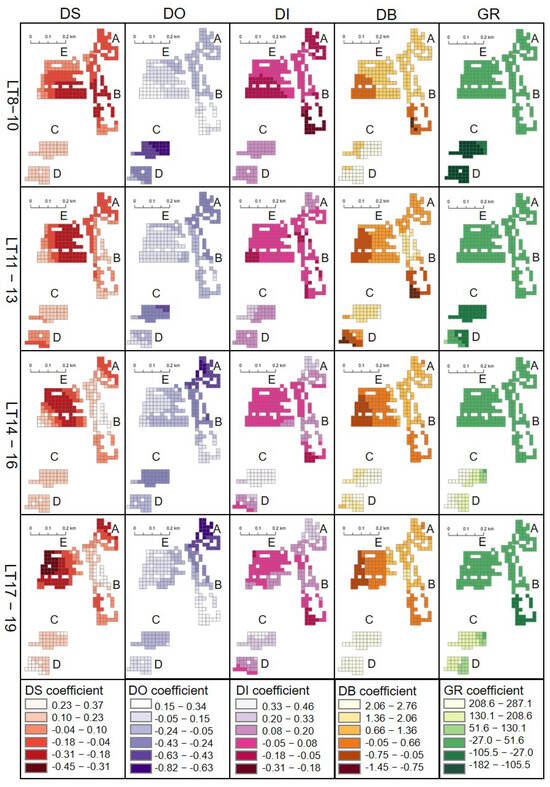
Figure 10.
Local regression results of spatial influencing factors on near-surface CO2 in urban communities during different time periods.
The quantitative analysis revealed significant traffic-related impacts on community-scale CO2 dynamics. Distance to Intersections (DI) demonstrated marked regression coefficients during LT8–10 (morning peak) in Communities A, B, and E (β = −0.31–0.1, p < 0.01), indicating substantial impacts of internal road proximity on CO2 concentrations, highlighting residents’ commuting behaviors. Distance to External Roads (DO) emerged as a critical predictor for Community C during LT8–10 (β = −0.62) and Community A at LT14–19 (evening peak, β = −0.82), suggesting elevated sensitivity to through-traffic emissions during rush hours.
Notably, DB exhibited dual-phase influences: positive correlations during LT11–13 in Community B (β = −1.45) and Community D (β = −0.75). Spatial analysis identified persistent dark hotspots (Figure 9) where DB-associated CO2 emissions peaked during lunch (12:00–14:00) and dinner (18:00–20:00) periods. This phenomenon correlates with the prevalent use of centralized exhaust ducts in these communities’ residential kitchens (85.7% adoption rate).
The Green Space Ratio (GR) exhibited dual-phase regulation of near-surface CO2 concentrations, demonstrating suppression effects during daytime and enhancement effects during evening-night period. This diurnal phasic alternation aligns with vegetation’s photosynthetic assimilation and respiratory release processes [49,50,51,52]. Meanwhile, this result also indicates that the green spaces within cities should not be considered merely as carbon sink elements. In fact, the green spaces undergo a transformation process from carbon source to carbon sink over time. Vegetation coverage displayed elevated regression coefficients (β = 130.1–208.6, p < 0.05) in Communities C and D, suggesting that while the carbon sequestration capacity of green-blue infrastructure remains limited compared to traffic-related sources (β = −0.18 ± 0.64) and household energy emissions (β = 0.65 ± 2.11), strategic greening interventions can amplify CO2 mitigation efficiency.
5. Discussion
5.1. Spatiotemporal Pattern Typology
The above findings revealed significant spatiotemporal heterogeneity in near-surface CO2 distributions across the five community types. Community A (high-rise apartments) exhibited the highest mean CO2 concentration, peaking in the evening with pronounced diurnal fluctuations (LT8–13), classified as an externally dominated high-concentration community. Its elevated CO2 levels were primarily influenced by external traffic and green space ratio. Community E (newly built residential complexes) showed the second-highest mean concentration but displayed a bimodal temporal pattern with morning peaks (LT7–10 and LT13–17), representing an internally dominated high-concentration type. Its CO2 dynamics were strongly associated with road intersections. Communities C (row houses) and D (urban villages) demonstrated similar mean concentrations with evening maxima and afternoon minima. Community C exhibited significant spatial heterogeneity with elevated concentrations near roads, suggesting limited vertical/horizontal diffusion due to external traffic impacts. Notably, green spaces in Community C paradoxically enhanced CO2 levels rather than mitigating them, potentially due to restricted airflow from shrub vegetation. Conversely, Community D displayed concentrated hotspots in interior zones, primarily influenced by internal traffic and domestic energy consumption patterns. Community B (villa district) maintained the lowest mean concentrations, particularly during LT11–13, with morning peaks and evening secondary elevations. Its riverside green spaces showed the minimum CO2 concentrations spatially.
5.2. Differential Driver Mechanisms
The analysis identified AH as a significant factor positively correlated with near-surface CO2 concentrations, explaining why high-rise apartments (Type A) and commercial complexes (Type E) exhibited the highest CO2 levels. This finding corresponds with Tian et al.’s observation that building height strongly influences residential and traffic-related CO2 emissions [53]. Additionally, the ED index demonstrated robust correlations with afternoon and evening CO2 levels, highlighting that enclosed urban forms obstruct effective carbon dispersion.
While prior studies primarily focused on the impact of road traffic on residential CO2 emissions [54], our findings shed light on how spatial drivers vary across different community types. In Type A and Type C communities, external traffic acted as the primary contributor to CO2 levels, whereas in Types B, D, and E, internal traffic and household energy use were the dominant sources. These findings align with earlier research identifying home heating and vehicular traffic as major anthropogenic sources of urban CO2 emissions [55], providing a more nuanced perspective on how spatial factors drive CO2 variation in diverse urban communities.
Contrary to the widely held perception of green spaces as universal carbon sinks, their carbon sequestration efficiency varies significantly between community types. While effective in reducing CO2 levels in Type A and Type B communities, green spaces in Type C communities paradoxically contributed to elevated CO2 concentrations. This unexpected result can be attributed to the limited carbon sequestration capacity of urban vegetation, intensified by nocturnal plant respiration and restricted CO2 diffusion caused by dense vegetation structures.
Urban green spaces generally exhibit limited carbon sequestration capability, offsetting less than 2% of total CO2 emissions at the community level [3]. In high-density areas, green spaces are often small, overly compact, and sparsely distributed [56], resulting in inherently low sequestration rates. The issue is further compounded by high anthropogenic emissions from building energy use and human respiration, which can overpower the carbon absorption function of urban vegetation. Nocturnal plant respiration also significantly impacts localized CO2 levels. In communities with dense or poorly planned vegetation arrangements, such as Type C, nocturnal respiration contributes substantially to CO2 emissions. For instance, data from Zurich’s CO2 monitoring network revealed that the highest CO2 concentrations coincided with areas experiencing intense nocturnal plant respiration [57].
Furthermore, studies have shown that the spatial configuration and structural characteristics of vegetation critically influence its carbon absorption capacity [58]. In Type C communities, dense shrub vegetation often creates physical barriers to both horizontal and vertical air circulation. Computational Fluid Dynamics (CFD) simulations [59] indicate that dense vegetation, including evergreen shrubs, vines, and lawns, can hinder airflow under calm or low-wind conditions, exacerbating the localized accumulation of CO2.
5.3. Practical Mitigation Pathways
The findings strongly suggest the necessity for developing tailored carbon management strategies for different community types to mitigate near-surface CO2 concentrations and advance sustainable urban development. The recommendations focus on three aspects: spatial organization, green landscape design, and policy guidelines.
- (1)
- Optimization of spatial organization
Urban planning and community design are expected to prioritize the optimization of spatial configurations to facilitate airflow and reduce CO2 concentrations. This involves controlling critical spatial parameters that influence air movement and carbon emission dynamics.
Firstly, improving spatial morphology is essential for enhancing air circulation. In the context of urban renewal or the design of new communities, attention should be given to building layouts to control levels of enclosure and openness. For example, reducing the enclosure degree can promote optimal airflow near the ground surface. In high-concentration areas such as Type A and Type E communities, lowering building heights can minimize obstructions to air circulation and encourage better natural air convection, enabling the effective dispersion of CO2.
Additionally, the internal organization of community functions plays a crucial role in reducing emissions from transportation. Communities can adopt the “15 min walkable community” principle to enhance the functional diversity and accessibility of daily services, reducing resident dependency on motorized commuting [60]. Shorter commutes not only decrease travel distances and time but also mitigate carbon emissions directly at their source. Specific measures, such as traffic flow regulation during peak hours (e.g., at LT7–9 and LT17–19 in Type A communities), can further alleviate the carbon footprint of urban transportation.
- (2)
- Green landscape design and carbon sequestration enhancement
Green landscape design serves as a critical component of community carbon management, contributing to both carbon sequestration and localized CO2 dispersion. Various strategies can be employed to maximize its effectiveness.
The first recommendation is to allocate dedicated carbon sink spaces. For high-density urban renewal initiatives and new community developments, reserving 10–15% of the total community area for carbon sink landscapes is advised. In Type A and Type B communities, implementing strategic green coverage of at least 25% can not only offset emissions from traffic and daily activities, but also enhance localized CO2 dispersion conditions [48].
Strategic vegetation planning is another critical measure. Urban green spaces should prioritize plant species with high carbon absorption efficiency [61], customized to the local climatic conditions. In Type C communities, planners should avoid overly dense shrub vegetation, which can impede airflow. Instead, adjustments to the ratio of grassland to trees can improve CO2 dispersion at the ground level while enhancing carbon storage capacity [62].
Integrating vertical and rooftop greening into architectural design represents a further step toward more effective community-wide carbon sequestration. Vertical greening of building facades, combined with rooftop greening systems, can not only increase vegetation’s ability to absorb CO2, but also enhance airflow along building surfaces [63,64]. This synergy improves near-surface CO2 diffusion, leading to substantial enhancements in localized air quality and overall carbon management efficiency.
- (3)
- Policy guidelines and regulatory frameworks
To ensure implementation of these carbon management strategies, it is vital to establish clear policy guidelines and regulatory standards. Near-surface CO2 concentration thresholds (e.g., less than 450 ppm) should be integrated into community planning and design standards as mandatory requirements for new construction and redevelopment projects. These thresholds would ensure stricter adherence to carbon reduction goals across communities.
5.4. Limitations
This study has three primary limitations. One limitation of this research lies in its restricted analysis of seasonal variation in near-surface CO2 concentrations. The CO2 measurement data were primarily collected during the spring, a season characterized by relatively stable atmospheric conditions near the surface. This ensured the reliability and representativeness of the data, providing a sound basis for analyzing the relationship between spatial forms and CO2 concentrations. However, the lack of data from other seasons prevents the full characterization of seasonal dynamics in CO2 concentrations. For instance, during the winter, heating activities generate additional emissions that may lead to significantly elevated CO2 concentrations. Consequently, the study might underestimate the specific concentration patterns of winter, limiting the generalizability of its conclusions.
This study also has some methodological constraints. For instance, the study employed both mobile measurement devices (TSI-7525) and fixed sensors (Qingping), which have a measurement error margin of ±15 ppm. Despite implementing several calibration and data control strategies, this measurement variability introduces potential uncertainties in data precision. Meanwhile, the study’s spatial scope was confined to a 1 km2 survey area, with typological analyses covering only five representative community types (A through E). The diversity of community structures in other urban settings may not be fully captured within this study’s scope. Thus, the applicability of the conclusions might be limited in cities with a broader range of community typologies and climatic conditions.
Finally, there were some certain extraneous variables that were beyond the scope of quantification might have influenced the measured near-surface CO2 concentrations. For example, temporary human activities, such as nighttime street markets in Type A communities, can significantly elevate local emission levels. However, due to their transient and dynamic nature, these factors were not systematically accounted for in the analysis.
To address the above limitations and enhance the robustness of the findings, future studies will focus on incorporating seasonal and temporal variations, as well as integrating remote sensing and big data analysis. We will include CO2 measurements conducted during different seasons, combining routine weekdays and weekends. This approach aims to capture the spatiotemporal variations in near-surface CO2 concentrations in high-density urban environments, thereby improving the generalizability and representativeness of the study conclusions. Furthermore, remote sensing technologies will be integrated with urban big data analytics to enhance the spatial and temporal resolution of CO2 monitoring.
6. Conclusions
This study uncovers three fundamental characteristics of near-surface CO2 distributions in heterogeneous urban communities and provides important insights into localized carbon management. By employing high spatiotemporal resolution measurements, we analyzed CO2 concentrations across five distinct urban residential typologies, advancing the understanding of how spatial factors influence urban carbon dynamics. Specifically, our investigation achieved a temporal resolution of hourly intervals and a spatial resolution of 20 m grid cells for CO2 monitoring. Compared to traditional urban CO2 monitoring techniques utilizing eddy covariance (EC) systems—typically with spatial footprints ranging from 100 m to 1 km—our study significantly enhances both the temporal and spatial precision of near-surface CO2 data.
In terms of carbon emission drivers, prior research has predominantly examined the macro-level phenomenon in which residential proximity to external roads correlates with elevated CO2 concentrations. However, our findings reveal pronounced differences in the impact of spatial elements across various community typologies. For high-rise apartment complexes and row-house residential areas, external traffic emissions predominantly drive CO2 concentrations. In contrast, internal circulation of vehicles and household energy consumption are stronger determinants of carbon emissions in villa districts, urban villages, and residential complexes. Additionally, the effects of green space ratio vary across different configurations. While green spaces significantly reduce CO2 concentrations in well-ventilated community, they paradoxically contribute to concentration increases in other community types, underscoring the importance of context-specific green infrastructure planning.
These findings provide an empirical foundation for spatially explicit carbon management, highlighting the urgent need for typology-specific carbon mitigation strategies. Optimizing spatial configurations—such as adjusting building heights, managing enclosure degrees, and strategically placing green infrastructures—can effectively reduce CO2 concentrations across diverse community types. Complementary measures, such as integrated traffic flow management during peak hours (07:00–09:00 and 17:00–19:00 LT) and energy-efficient retrofitting of residential infrastructure, present significant potential for driving progress toward urban carbon neutrality.
The holistic integration of spatial optimization, green landscape design, and policy innovation offers a comprehensive pathway for effective carbon management across urban communities. By addressing both natural and anthropogenic sources of CO2, these measures not only reduce CO2 levels but also facilitate long-term sustainable urban development. Tailored strategies designed for the unique spatial characteristics of different communities provide cities with the tools to construct adaptive and robust decarbonization frameworks, thereby laying the foundation for future low-carbon urban growth.
Author Contributions
Conceptualization, Y.W. and Y.Z.; methodology, Y.W., Y.Z. and B.S.; software, Y.W. and Q.Y.; validation, Y.Z., B.S. and C.G.; formal analysis, Y.W. and J.L.; investigation, Y.W., J.L., Y.Z. and Q.Y.; resources, Y.Z.; data curation, Y.W.; writing—original draft preparation, Y.W. and Y.Z.; writing—review and editing, Y.W., Y.Z., W.D. and B.S.; visualization, Y.W. and Y.Z.; supervision, Y.Z. and C.G.; project administration, Y.Z.; funding acquisition, Y.Z. and C.G. All authors have read and agreed to the published version of the manuscript.
Funding
This research was funded by the National Natural Science Foundation of China, grant number 52394224; The Young Elite Scientists Sponsorship Program by China Association for Science and Technology, grant number 2022QNRC001-YESS20220569; Shanghai Key Laboratory of Urban Design and Urban Science, NYU Shanghai Open Topic Grants, grant number 2023YZheng_LOUD and Key Laboratory of Ecology and Energy Saving Study of Dense Habitat Open Topic Grants, grant number 20240110.
Data Availability Statement
The data that support the findings of this study are available from the first author upon reasonable request. Researcher that would like to obtain the data mentioned in this article for research purposes should contact wyy_2023@seu.edu.cn for data acquisition according to the data usage requirements.
Conflicts of Interest
The authors declare no conflicts of interest.
Abbreviations
The following abbreviations are used in this manuscript:
| AH | Average Height |
| BA | Building Area |
| BD | Building Density |
| DB | Distance to Buildings |
| DI | Distance to the Intersection |
| DO | Distance to the Outer Road |
| DS | Distance to the community Street |
| ED | Enclosure Degree |
| FAR | Floor Area Ratio |
| GPS | Global Positioning System |
| GTWR | Geographically and Temporally Weighted Regression |
| GWR | Geographically Weighted Regression |
| LT | Local Time |
| MH | Max Height |
| NDIR | Non-Dispersive Infra-Red |
| OLS | Ordinary Least Square |
| OSR | Open Space Ratio |
| PA | Plot Area |
| PP | Plot Perimeter |
| RMA | Regression Moving Average |
| RF | Random Forest |
| TBA | Total Building Area |
Appendix A
Appendix A.1. Indicator Calculation
The aim of this study is to investigate the distribution patterns of CO2 and the spatiotemporal differentiation characteristics in different types of residential communities within high-density urban environments. The classification criteria for the communities in this study reference the Local Climate Zones (LCZ) classification system developed by Stewart and Oke, which is widely used to describe and categorize various climatic regions in urban areas. Additionally, relevant conclusions from existing research on the influencing factors of CO2 concentration were considered, leading to the establishment of a comprehensive indicator system consisting of four aspects: plot indicators, morphological indicators, density indicators, and layout indicators.
Specifically, the plot indicators are used to quantify the overall planar morphology of residential communities, influencing the inflow and outflow of climate resources and CO2 emissions, including the area and perimeter of the communities. Secondly, the morphological indicators quantify the three-dimensional morphological characteristics of high-density residential plots. The distribution of building footprints and their vertical arrangement affect the airflow around the environment and the diffusion and distribution of CO2. We selected the total footprint area (the sum of all building footprints within the plot), total building area (the sum of the total building areas within the plot), average height (the average height of all buildings within the plot), and maximum height (the height of the tallest building within the plot).
The density indicators quantify the spatial aggregation degree, influencing the accumulation and concentration of CO2. We selected building density (the ratio of building area to plot area), floor area ratio (the ratio of total building area to plot area), and the proportion of open space (the ratio of green space area to plot area). The layout indicators include block enclosure degree (the total building footprint area within a ten-meter circular buffer zone inward from the plot boundary relative to the plot area) and building layout forms (linear, enclosed, clustered, and mixed). These indicators comprehensively consider the relationship between the neighborhood and the near-surface atmospheric circulation, where a reasonable layout facilitates ventilation, CO2 diffusion, and concentration reduction.
Appendix A.2. Data Acquisition
In the process of defining residential area types, the data utilized can be categorized into four main types: community information data, building data, green space data, and road data (see detailed data information in Table A1). The data used in this study is open-source data, and all data can be obtained from the respective platform providers. Detailed acquisition methods can be found in the respective data website links.
Table A1.
Data list.
Table A1.
Data list.
| Data Name | Data Content | Year | Data Sources | Application |
|---|---|---|---|---|
| Community Information Data | Housing Name, Year of Construction, Number of Households, Boundary | 2022 | China’s largest second-hand housing transaction website | Obtain boundaries and calculate plot indicators |
| Building Data | Building Area, Number of Floors | 2021 | Tianditu Platform | Morphological, density, and layout indicators |
| Green Space Data | Green Space Area Vector Outline | 2021 | Tianditu Platform | Calculate density indicators |
| Road Data | Road Centerline Vector | 2021 | Amap (Gaode Map) Platform | Correct community boundaries |
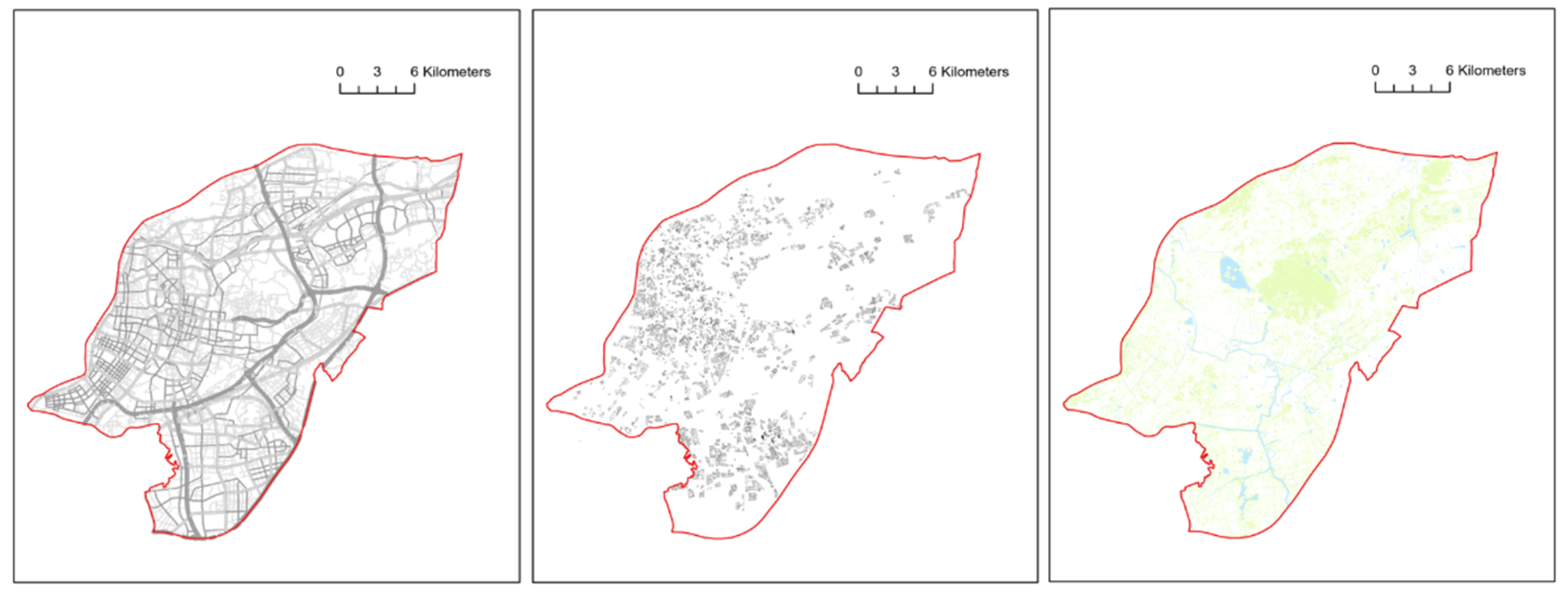
Community information data are sourced from Beike, China’s largest second-hand housing transaction website (https://nj.ke.com/). Building data and green space data are sourced from the Tianditu platform (https://www.tianditu.gov.cn/). This study assumes a height of 3 m per floor, meaning the building height is calculated as the number of floors multiplied by 3 m. Road data are sourced from the Amap (Gaode Map) platform in this study, and are combined with the latest satellite imagery and street view pictures to correct the community boundaries. Finally, building data are spatially linked with the corrected boundaries in the ArcGIS Pro platform to identify residential buildings in the central urban area of Nanjing (see research scope in Figure A1 and community boundaries in Figure A2) and calculate the morphological indicators of the residential areas.
The results of the indicator calculations are standardized, and linear transformations are applied to the series of spatial morphology data to convert both positive and negative indicators into positive indicators, ensuring that their directional effects are consistent and facilitating comparison.
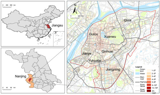
Figure A1.
Research scope.
Figure A1.
Research scope.
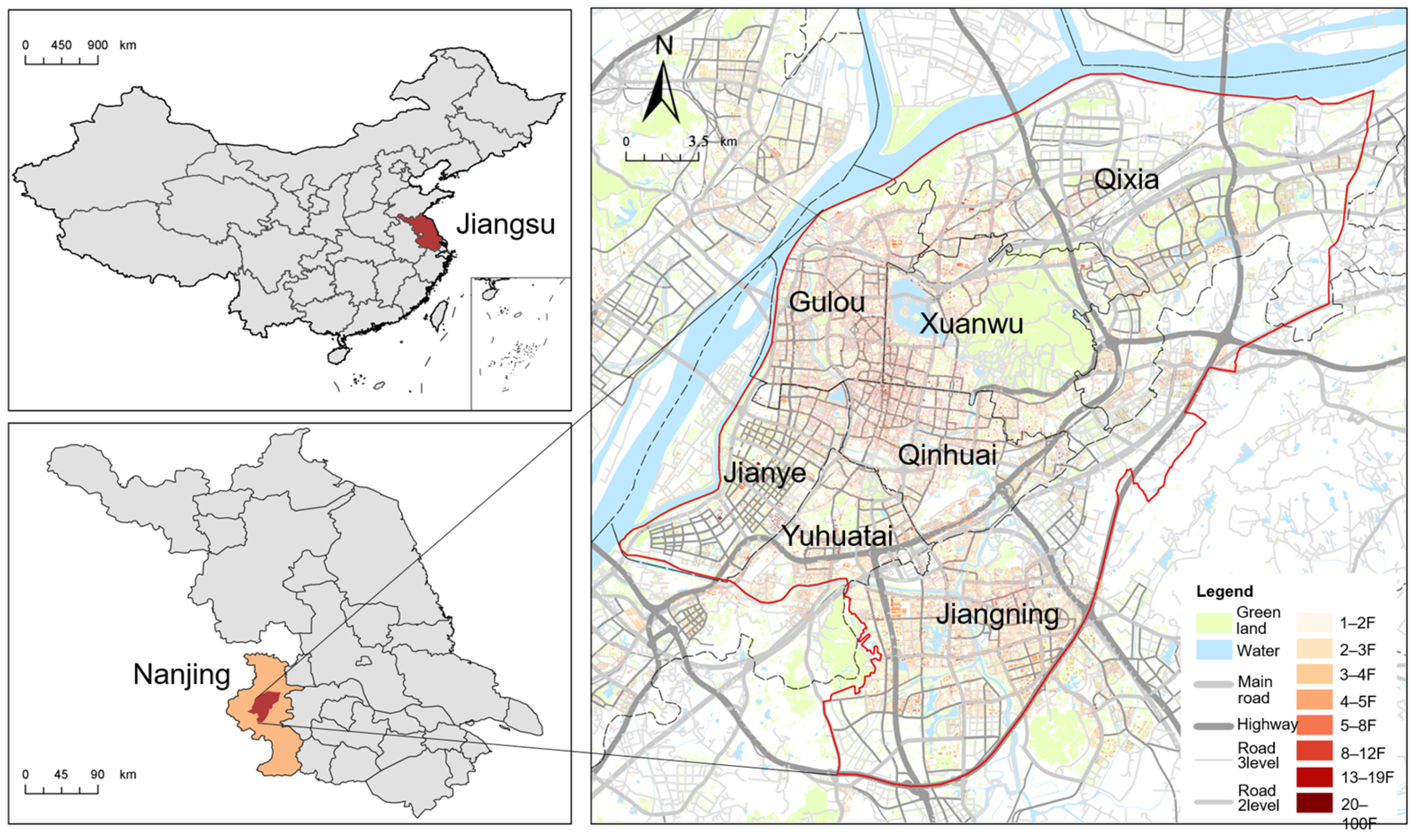
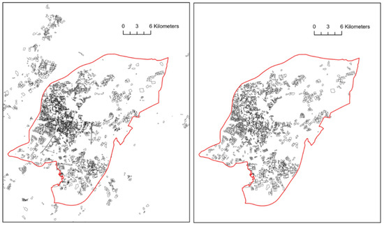
Figure A2.
Residential community boundaries before and after correction.
Figure A2.
Residential community boundaries before and after correction.
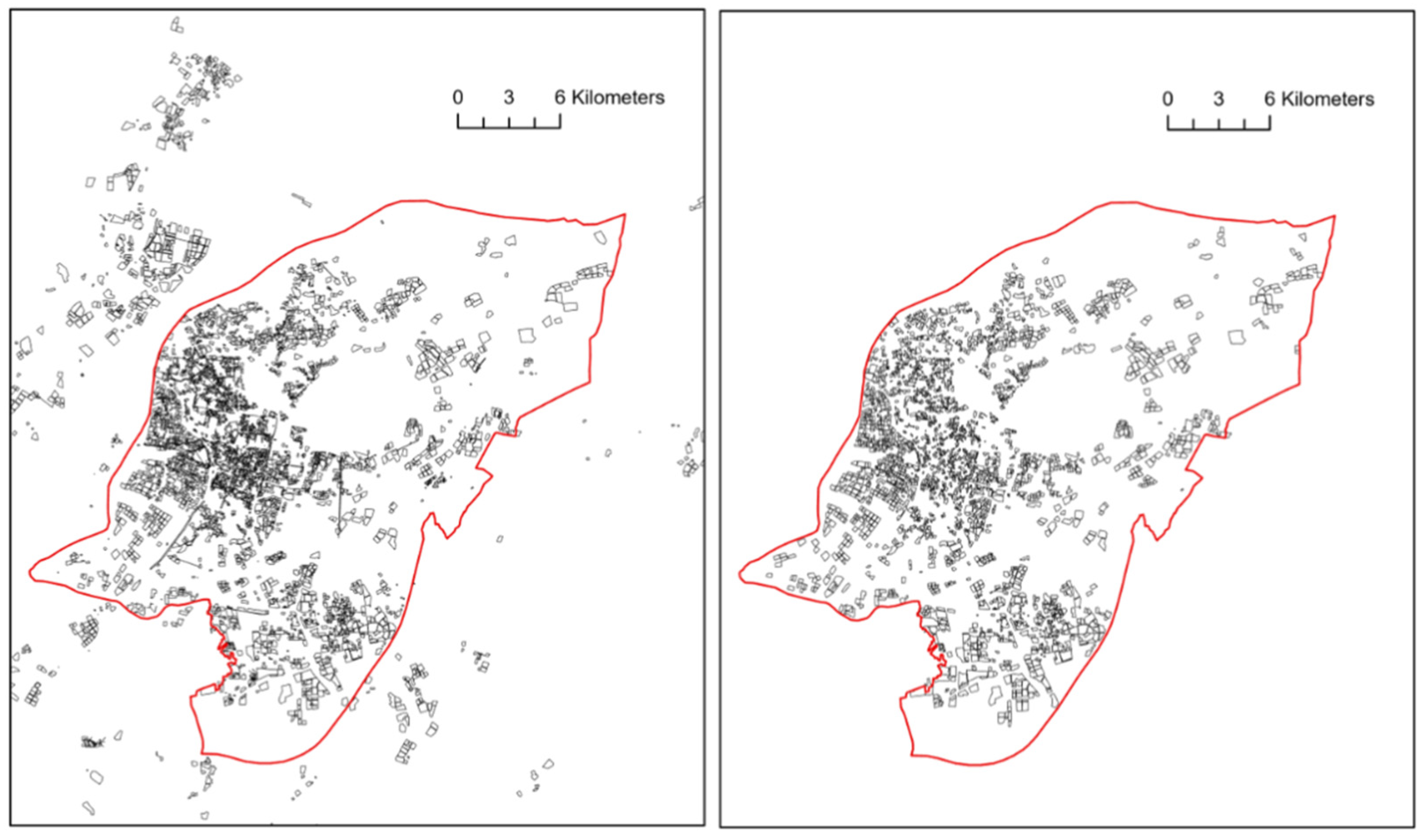
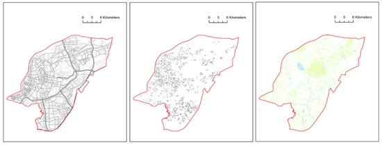
Figure A3.
Distribution of residential buildings, roads, and green spaces.
Figure A3.
Distribution of residential buildings, roads, and green spaces.
Appendix A.3. Clustering Methods and Results
The study used K-means unsupervised clustering to cluster spatial morphology indicators. This clustering method is chosen because of its high reliability, computational efficiency, and ease of implementation. Existing studies have demonstrated that K-means has high accuracy in fitting spatial morphology, effectively identifying the characteristics of different spatial forms. Therefore, the credibility and validity of the research results can be ensured, providing a solid foundation for subsequent analysis.
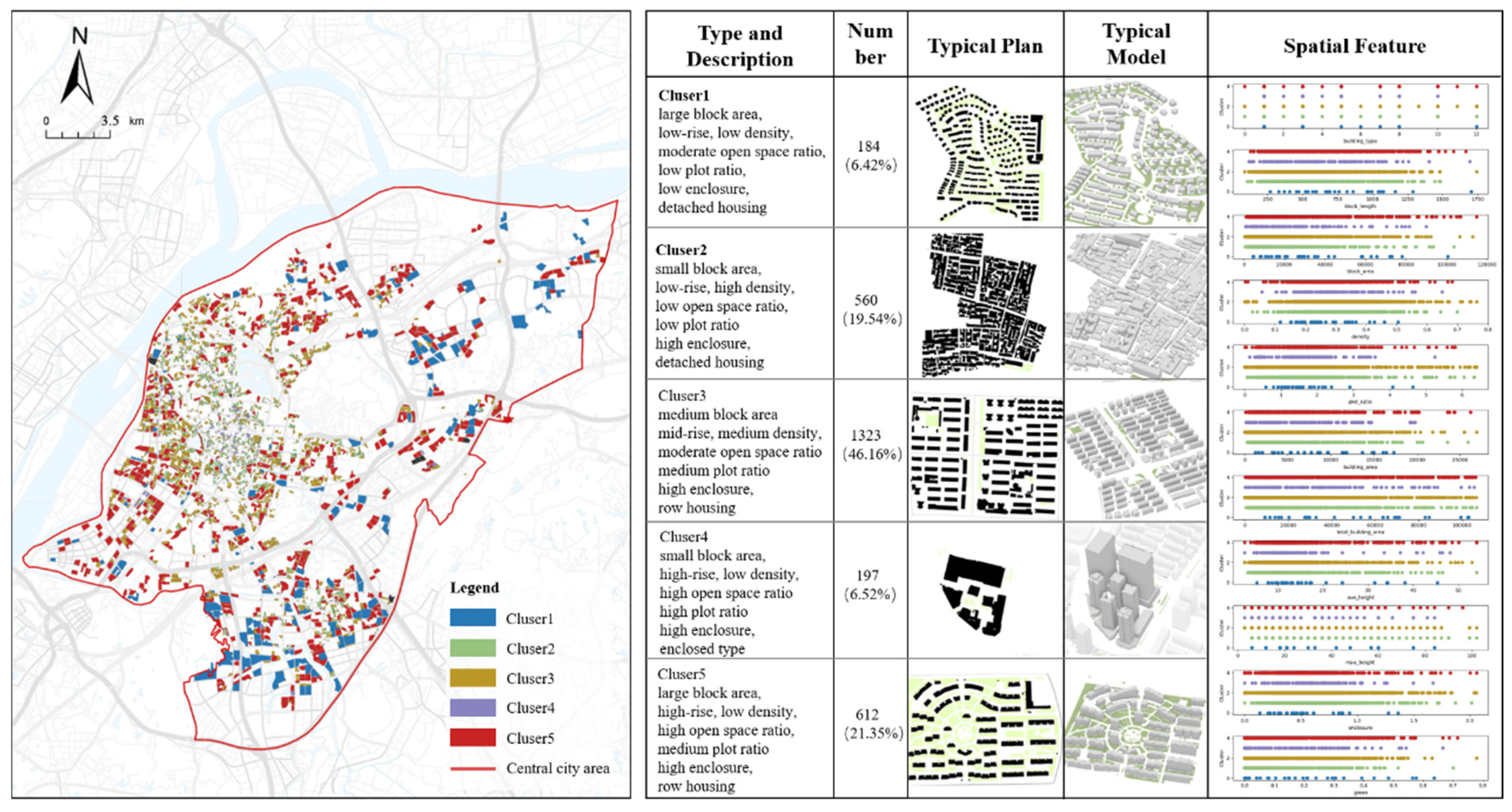
The results show that there are five different types of residential plots in the central urban area of Nanjing, which can be characterized as: villa communities; urban village communities; row houses; high-rise apartments; and typical newly built commercial apartment complexes. There are 184 villa communities, consisting of low-rise detached housing. The villa community has a large block area, moderate open space ratio, and features low plot ratio, low density, and low enclosure. There are 560 urban village communities, consisting of low-rise detached housing. The urban village community has a small block area and low open space ratio, and is characterized by low plot ratio, high density, and high enclosure. There are 1323 row houses, consisting of mid-rise row housings. The row house has a medium block area, the open space ratio is moderate, and it has the characteristics of medium plot ratio, medium density, and high enclosure; There are 197 high-rise apartments, consisting of enclosed high-rise residential buildings. The high-rise apartment has small block area and has high open space radio, with characteristics of high plot ratio, low density, and high enclosure. There are 612 typical newly built commercial apartment complexes, consisting of high-rise row housings with large block area and a high open space ratio. It has the characteristics of medium plot ratio, low density, and high enclosure. The specific morphological characteristics of various types of residential plots are shown in Figure A4.
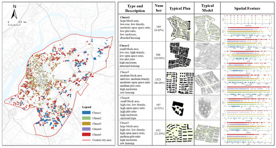
Figure A4.
Distribution of clustering results and characteristics of five types of residential communities.
Figure A4.
Distribution of clustering results and characteristics of five types of residential communities.
Appendix B
Table A2.
Feature importance of spatial distribution influencing factors.
Table A2.
Feature importance of spatial distribution influencing factors.
| Factors | ALL | Community A | Community B | Community C | Community D | Community E |
|---|---|---|---|---|---|---|
| DO | 0.256 | 0.390 | 0.220 | 0.479 | 0.182 | 0.201 |
| DS | 0.249 | 0.135 | 0.201 | 0.186 | 0.336 | 0.185 |
| DI | 0.209 | 0.249 | 0.247 | 0.154 | 0.345 | 0.366 |
| DB | 0.156 | 0.128 | 0.221 | 0.141 | 0.138 | 0.127 |
| GR | 0.130 | 0.099 | 0.111 | 0.040 | 0.000 | 0.121 |
| RMSE | 0.183 | 0.252 | 0.245 | 0.097 | 0.653 | 0.252 |
| R2 | 0.817 | 0.748 | 0.756 | 0.903 | 0.347 | 0.748 |
Appendix C
The Climatic Conditions on the Measurement Day
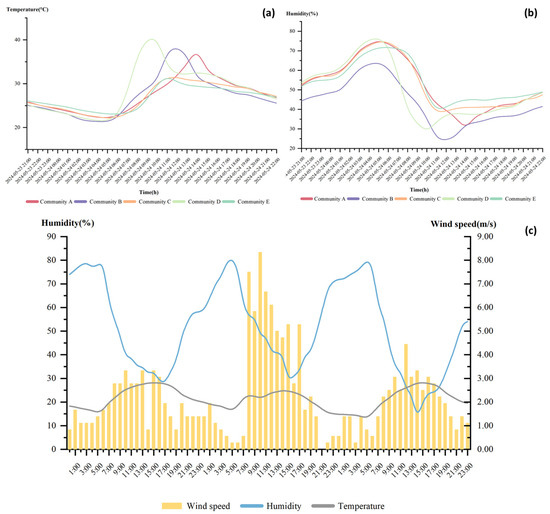
Figure A5.
Climatic information during the measurement period: (a) humidity (%) of different communities; (b) temperature (°C) of different communities; (c) temperature, humidity, and wind speed recorded at local weather stations during the study period.
Figure A5.
Climatic information during the measurement period: (a) humidity (%) of different communities; (b) temperature (°C) of different communities; (c) temperature, humidity, and wind speed recorded at local weather stations during the study period.
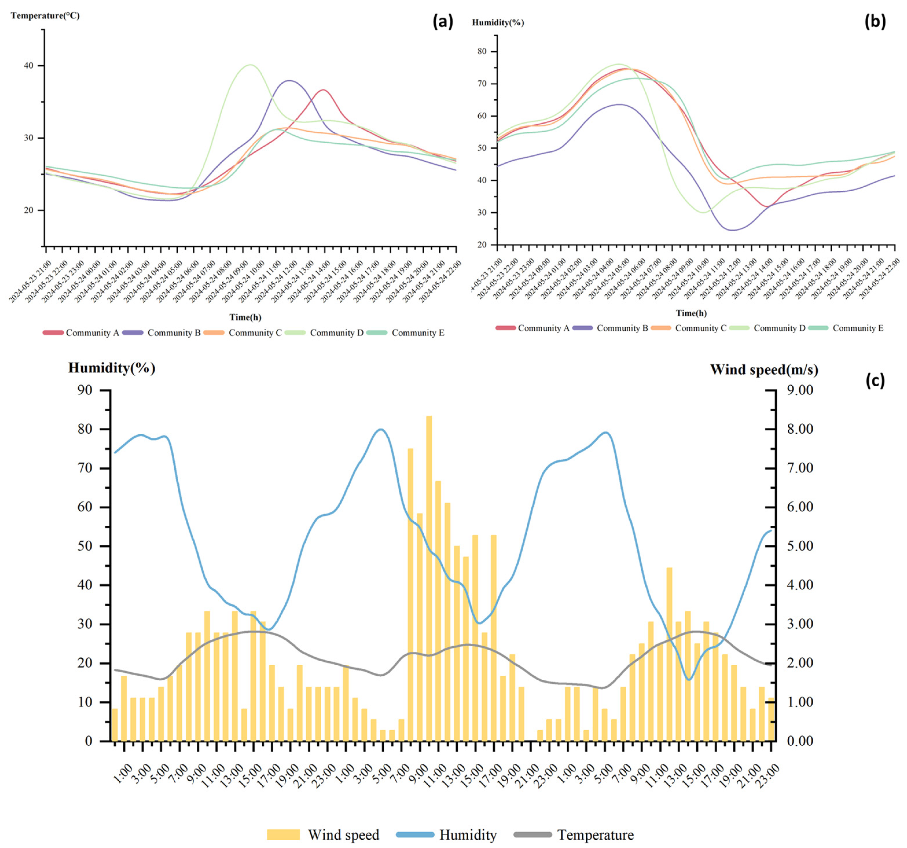
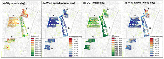
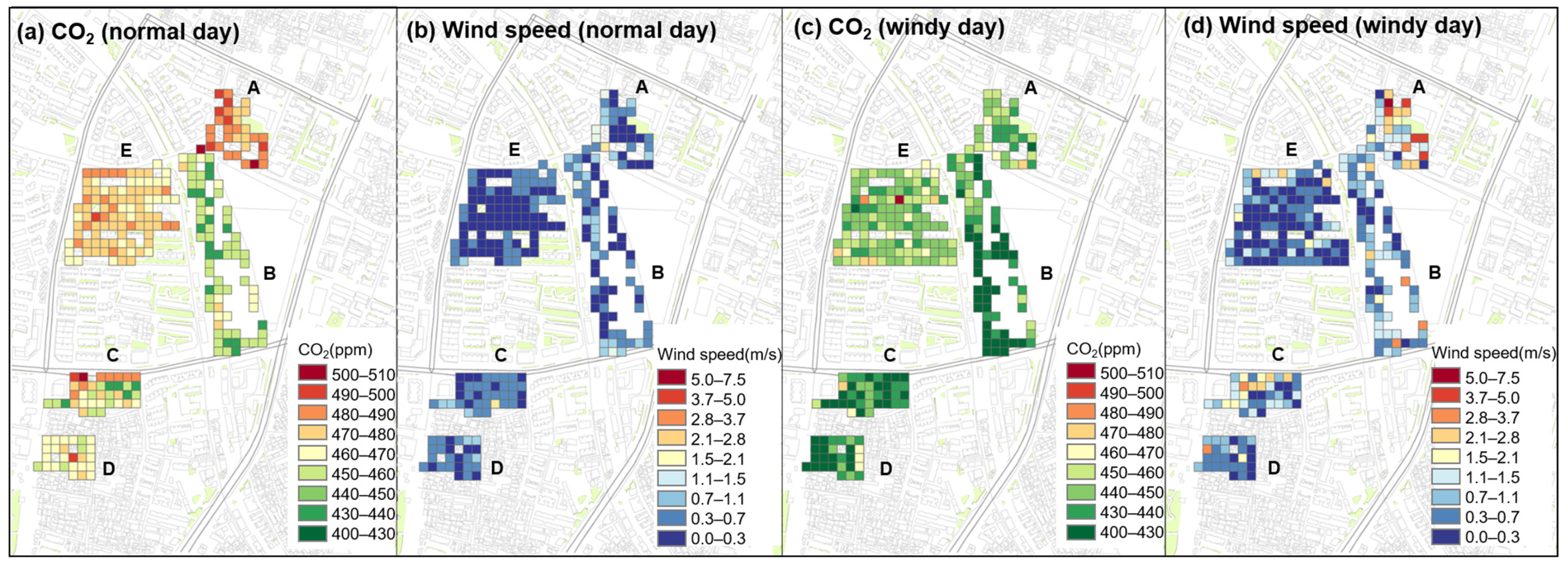
Figure A6.
Wind speed and CO2 distribution during windy weather: (a) average CO2 level distribution on common weather; (b) wind speed distribution on common weather; (c) average CO2 level distribution on windy weather; (d) wind speed distribution on windy weather.
Figure A6.
Wind speed and CO2 distribution during windy weather: (a) average CO2 level distribution on common weather; (b) wind speed distribution on common weather; (c) average CO2 level distribution on windy weather; (d) wind speed distribution on windy weather.
References
- Liu, J.; Zheng, X.; Chen, Y. Healthy and Low-Carbon Communities: Design, Optimization, and New Technologies. Build. Simul. 2023, 16, 1583–1585. [Google Scholar] [CrossRef]
- Goret, M.; Masson, V.; Schoetter, R.; Moine, M.-P. Inclusion of CO2 Flux Modelling in an Urban Canopy Layer Model and an Evaluation over an Old European City Centre. Atmos. Environ. X 2019, 3, 100042. [Google Scholar] [CrossRef]
- Cheng, J.; Mao, C.; Huang, Z.; Hong, J.; Liu, G. Implementation Strategies for Sustainable Renewal at the Neighborhood Level with the Goal of Reducing Carbon Emission. Sustain. Cities Soc. 2022, 85, 104047. [Google Scholar] [CrossRef]
- Kinnunen, A.; Talvitie, I.; Ottelin, J.; Heinonen, J.; Junnila, S. Carbon Sequestration and Storage Potential of Urban Residential Environment—A Review. Sustain. Cities Soc. 2022, 84, 104027. [Google Scholar] [CrossRef]
- Xiao, Z.; Ge, H.; Lacasse, M.A.; Wang, L.; Zmeureanu, R. Nature-based solutions for carbon neutral climate resilient buildings and communities: A review of technical evidence, design guidelines, and policies. Buildings 2023, 13, 1389. [Google Scholar] [CrossRef]
- Estruch, C.; Curcoll, R.; Morguí, J.-A.; Segura-Barrero, R.; Vidal, V.; Badia, A.; Ventura, S.; Gilabert, J.; Villalba, G. Exploring how the heterogeneous urban landscape influences CO2 concentrations: The case study of the Metropolitan Area of Barcelona. Urban For. Urban Green. 2024, 99, 128438. [Google Scholar] [CrossRef]
- Hou, H.; Zhang, S.; Ding, Z.; Wang, Y. Temporal variation of near-surface CO2 concentrations over different land uses in Suzhou City. Environ. Earth Sci. 2016, 75, 1197. [Google Scholar] [CrossRef]
- Song, T.; Wang, Y.; Sun, Y. Estimation of carbon dioxide flux and source partitioning over Beijing, China. J. Environ. Sci. 2013, 25, 2429–2434. [Google Scholar] [CrossRef]
- Wu, K.; Davis, K.J.; Miles, N.L.; Richardson, S.J.; Lauvaux, T.; Sarmiento, D.P.; Balashov, N.V.; Keller, K.; Turnbull, J.; Gurney, K.R.; et al. The role of emissions and meteorology in driving CO2 concentrations in urban areas. Environ. Res. Lett. 2022, 17, 074035. [Google Scholar] [CrossRef]
- Park, M.S.; Joo, S.J.; Lee, C.S. Effects of an urban park and residential area on the atmospheric CO2 concentration and flux in Seoul, Korea. Adv. Atmos. Sci. 2013, 30, 503–514. [Google Scholar] [CrossRef]
- Ueyama, M.; Ando, T. Diurnal, weekly, seasonal, and spatial variabilities in carbon dioxide flux in different urban landscapes in Sakai, Japan. Atmos. Chem. Phys. 2016, 16, 14727–14740. [Google Scholar] [CrossRef]
- Wang, Q.; Imasu, R.; Arai, Y.; Ito, S.; Mizoguchi, Y.; Kondo, H.; Xiao, J. Sub-daily natural CO2 flux simulation based on satellite data: Diurnal and seasonal pattern comparisons to anthropogenic CO2 emissions in the Greater Tokyo Area. Remote Sens. 2021, 13, 2037. [Google Scholar] [CrossRef]
- Di Martino, R.M.R.; Gurrieri, S. Theoretical principles and application to measure the flux of carbon dioxide in the air of urban zones. Atmos. Environ. 2022, 288, 119302. [Google Scholar] [CrossRef]
- Christen, A.; Coops, N.C.; Crawford, B.R.; Kellett, R.; Liss, K.N.; Olchovski, I.; Tooke, T.R.; van der Laan, M.; Voogt, J.A. Validation of modeled carbon-dioxide emissions from an urban neighborhood with direct eddy-covariance measurements. Atmos. Environ. 2011, 45, 6057–6069. [Google Scholar] [CrossRef]
- Liu, M.; Zhu, X.; Pan, C.; Chen, L.; Zhang, H.; Jia, W.; Xiang, W. Spatial variation of near-surface CO2 concentration during spring in Shanghai. Atmos. Pollut. Res. 2016, 7, 31–39. [Google Scholar] [CrossRef]
- Buckley, S.M.; Mitchell, M.J.; McHale, P.J.; Millard, G.D. Variations in carbon dioxide fluxes within a city landscape: Identifying a vehicular influence. Urban Ecosyst. 2016, 19, 1479–1498. [Google Scholar] [CrossRef]
- Gao, Y.; Lee, X.; Liu, S.; Hu, N.; Wei, X.; Hu, C.; Liu, C.; Zhang, Z.; Yang, Y. Spatiotemporal variability of the near-surface CO2 concentration across an industrial-urban-rural transect, Nanjing, China. Sci. Total Environ. 2018, 631–632, 1192–1200. [Google Scholar] [CrossRef]
- Björkegren, A.; Grimmond, C.S.B. Net carbon dioxide emissions from central London. Urban Clim. 2018, 23, 131–158. [Google Scholar] [CrossRef]
- Kim, M.K.; Choi, J.-H. Can increased outdoor CO2 concentrations impact ventilation and energy in buildings? A case study in Shanghai, China. Atmos. Environ. 2019, 210, 220–230. [Google Scholar] [CrossRef]
- Sensuła, B.; Chmura, L.; Necki, J.; Zimnoch, M. Insights from the last year’s atmospheric CO2 measurements in the urban atmosphere and the natural ecosystem in Southern Poland. Geochronometria 2024, 50, 206–222. [Google Scholar] [CrossRef]
- Velasco, E.; Segovia, E.; Roth, M. High-resolution maps of carbon dioxide and moisture fluxes over an urban neighborhood. Environ. Sci. Atmos. 2023, 3, 1110–1123. [Google Scholar] [CrossRef]
- Stagakis, S.; Chrysoulakis, N.; Spyridakis, N.; Feigenwinter, C.; Vogt, R. Eddy covariance measurements and source partitioning of CO2 emissions in an urban environment: Application for Heraklion, Greece. Atmos. Environ. 2019, 201, 278–292. [Google Scholar] [CrossRef]
- Ye, H.; Li, Y.; Shi, D.; Meng, D.; Zhang, N.; Zhao, H. Evaluating the potential of achieving carbon neutrality at the neighborhood scale in urban areas. Sustain. Cities Soc. 2023, 97, 104764. [Google Scholar] [CrossRef]
- Crawford, B.; Christen, A. Spatial variability of carbon dioxide in the urban canopy layer and implications for flux measurements. Atmos. Environ. 2014, 98, 308–322. [Google Scholar] [CrossRef]
- Liu, X.; Zhang, X.; Schnelle-Kreis, J.; Jakobi, G.; Cao, X.; Cyrys, J.; Yang, L.; Schloter-Hai, B.; Abbaszade, G.; Orasche, J.; et al. Spatiotemporal characteristics and driving factors of black carbon in Augsburg, Germany: Combination of mobile monitoring and street view images. Environ. Sci. Technol. 2021, 55, 160–168. [Google Scholar] [CrossRef]
- Baur, A.H.; Thess, M.; Kleinschmit, B.; Creutzig, F. Urban climate change mitigation in Europe: Looking at and beyond the role of population density. J. Urban Plan. Dev. 2014, 140, 94–95. [Google Scholar] [CrossRef]
- Cheshmehzangi, A.; Dawodu, A. Towards a sustainable energy planning strategy: The utilisation of floor area ratio for residential community planning and design in China. Front. Sustain. Cities 2021, 3, 687895. [Google Scholar] [CrossRef]
- Wang, M.; Zhang, F.; Wu, F. Governing urban redevelopment: A case study of Yongqingfang in Guangzhou, China. Cities 2022, 120, 103420. [Google Scholar] [CrossRef]
- Ohyama, H.; Frey, M.M.; Morino, I.; Shiomi, K.; Nishihashi, M.; Miyauchi, T.; Yamada, H.; Saito, M.; Wakasa, M.; Blumenstock, T.; et al. Anthropogenic CO2 emission estimates in the Tokyo metropolitan area from ground-based CO2 column observations. Atmos. Chem. Phys. 2023, 23, 15097–15119. [Google Scholar] [CrossRef]
- Zhu, X.-H.; Lu, K.-F.; Peng, Z.-R.; He, H.-D.; Xu, S.-Q. Spatiotemporal variations of carbon dioxide (CO2) at urban neighborhood scale: Characterization of distribution patterns and contributions of emission sources. Sustain. Cities Soc. 2022, 78, 103646. [Google Scholar] [CrossRef]
- Li, B.; Cao, R.; Wang, Z.; Song, R.-F.; Peng, Z.-R.; Xiu, G.; Fu, Q. Use of multi-rotor unmanned aerial vehicles for fine-grained roadside air pollution monitoring. Transp. Res. Rec. 2019, 2673, 169–180. [Google Scholar] [CrossRef]
- Park, C.; Jeong, S.; Park, H.; Kim, Y. Challenges in monitoring atmospheric CO2 concentrations in Seoul using low-cost sensors. Asia-Pac. J. Atmos. Sci. 2021, 57, 547–553. [Google Scholar] [CrossRef]
- Lu, K.F.; He, H.D.; Wang, H.W.; Li, X.B.; Peng, Z.R. Characterizing temporal and vertical distribution patterns of traffic-emitted pollutants near an elevated expressway in urban residential areas. Build. Environ. 2020, 172, 106678. [Google Scholar] [CrossRef]
- Bansal, P.; Quan, S.J. Relationships between building characteristics, urban form and building energy use in different local climate zone contexts: An empirical study in Seoul. Energy Build. 2022, 272, 112335. [Google Scholar] [CrossRef]
- Zhang, Y.; Zhou, W.; Ding, J. Effects of the Built Environment on Travel-Related CO2 Emissions Considering Travel Purpose: A Case Study of Resettlement Neighborhoods in Nanjing. Buildings 2022, 12, 1718. [Google Scholar] [CrossRef]
- Javadpoor, M.; Sharifi, A.; Gurney, K.R. Mapping the relationship between urban form and CO2 emissions in three US cities using the Local Climate Zones (LCZ) framework. J. Environ. Manag. 2024, 370, 122723. [Google Scholar] [CrossRef]
- Cader, J.; Koneczna, R.; Olczak, P. The impact of economic, energy, and environmental factors on the development of the hydrogen economy. Energies 2021, 14, 4811. [Google Scholar] [CrossRef]
- Yin, H.; Xiao, R.; Fei, X.; Zhang, Z.; Gao, Z.; Wan, Y.; Tan, W.; Jiang, X.; Cao, W.; Guo, Y. Analyzing “economy-society-environment” sustainability from the perspective of urban spatial structure: A case study of the Yangtze River delta urban agglomeration. Sustain. Cities Soc. 2023, 96, 104691. [Google Scholar] [CrossRef]
- Zhou, L.; Dang, X.; Sun, Q.; Wang, S. Multi-scenario simulation of urban land change in Shanghai by random forest and CA-Markov model. Sustain. Cities Soc. 2020, 55, 102045. [Google Scholar] [CrossRef]
- Khajavi, H.; Rastgoo, A. Predicting the carbon dioxide emission caused by road transport using a Random Forest (RF) model combined with meta-heuristic algorithms. Sustain. Cities Soc. 2023, 93, 104503. [Google Scholar] [CrossRef]
- Fotheringham, A.S.; Crespo, R.; Yao, J. Geographical and temporal weighted regression (GTWR). Geogr. Anal. 2015, 47, 431–452. [Google Scholar] [CrossRef]
- Park, C.; Jeong, S.; Kim, C.; Shin, J.; Joo, J. Machine learning based estimation of urban on-road CO2 concentration in Seoul. Environ. Res. 2023, 231 Pt 3, 116256. [Google Scholar] [CrossRef] [PubMed]
- Jiang, Y.; Sun, Y.; Liu, Y.; Li, X. Exploring the Correlation between Waterbodies, Green Space Morphology, and Carbon Dioxide Concentration Distributions in an Urban Waterfront Green Space: A Simulation Study Based on the Carbon Cycle. Sustain. Cities Soc. 2023, 98, 104831. [Google Scholar] [CrossRef]
- National Oceanic and Atmospheric Administration (NOAA). Global Monthly Mean CO2. Available online: https://gml.noaa.gov/ccgg/trends/global.html (accessed on 30 March 2025).
- Jardim, B.; de Castro Neto, M.; Calçada, P. Urban Dynamic in High Spatiotemporal Resolution: The Case Study of Porto. Sustain. Cities Soc. 2023, 98, 104867. [Google Scholar] [CrossRef]
- Gurney, K.; Romero-Lankao, P.; Seto, K.; Hutyra, L.R.; Duren, R.; Kennedy, C.; Grimm, N.B.; Ehleringer, J.R.; Marcotullio, P.; Hughes, S.; et al. Climate change: Track urban emissions on a human scale. Nature 2015, 525, 179–181. [Google Scholar] [CrossRef]
- Sun, D.J.; Zhang, Y.; Xue, R.; Zhang, Y. Modeling carbon emissions from urban traffic system using mobile monitoring. Sci. Total Environ. 2017, 599–600, 944–951. [Google Scholar] [CrossRef]
- Teng, W.; Shi, C.; Yu, Y.; Li, Q.; Yang, J. Uncovering the spatiotemporal patterns of traffic-related CO2 emission and carbon neutrality based on car-hailing trajectory data. J. Clean. Prod. 2024, 467, 142925. [Google Scholar] [CrossRef]
- Barichivich, J.; Briffa, K.R.; Myneni, R.B.; Osborn, T.J.; Melvin, T.M.; Ciais, P.; Piao, S.; Tucker, C. Large-scale variations in the vegetation growing season and annual cycle of atmospheric CO2 at high northern latitudes from 1950 to 2011. Glob. Change Biol. 2013, 19, 3167–3183. [Google Scholar] [CrossRef]
- Park, R.; Epstein, S. Carbon isotope fractionation during photosynthesis. Geochim. Cosmochim. Acta 1960, 44, 5–15. [Google Scholar] [CrossRef]
- Francey, R.J.; Tans, P.P. Latitudinal variation in oxygen-18 of atmospheric CO2. Nature 1987, 327, 495–497. [Google Scholar] [CrossRef]
- Fujita, D.; Ishizawa, M.; Maksyutov, S.; Thornton, P.E.; Saeki, T.; Nakazawa, T. Inter-annual variability of the atmospheric carbon dioxide concentrations as simulated with global terrestrial biosphere models and an atmospheric transport model. Tellus B Chem. Phys. Meteorol. 2003, 55, 530–546. [Google Scholar] [CrossRef]
- Tian, Y.; Zuo, S.; Ju, J.; Dai, S.; Ren, Y.; Dou, P. Local Carbon Emission Zone Construction in the Highly Urbanized Regions: Application of Residential and Transport CO2 Emissions in Shanghai, China. Build. Environ. 2024, 247, 111007. [Google Scholar] [CrossRef]
- Roth, M.; Jansson, C.; Velasco, E. Multi-year energy balance and carbon dioxide fluxes over a residential neighbourhood in a tropical city. Int. J. Climatol. 2017, 37, 2679–2698. [Google Scholar] [CrossRef]
- Bezyk, Y.; Sówka, I.; Górka, M. Assessment of Urban CO2 Budget: Anthropogenic and Biogenic Inputs. Urban Clim. 2021, 39, 100949. [Google Scholar] [CrossRef]
- Li, Z.; Chen, X.; Shen, Z.; Fan, Z. Evaluating Neighborhood Green-Space Quality Using a Building Blue–Green Index (BBGI) in Nanjing, China. Land 2022, 11, 445. [Google Scholar] [CrossRef]
- Grange, S.K.; Rubli, P.; Fischer, A.; Brunner, D.; Hueglin, C.; Emmenegger, L. The ZiCOS-M CO2 sensor network: Measurement performance and CO2 variability across Zurich. Atmos. Chem. Phys. 2025, 25, 2781–2806. [Google Scholar] [CrossRef]
- Zhang, X.; Huang, H.; Tu, K.; Li, R.; Zhang, X.; Wang, P.; Li, Y.; Yang, Q.; Acerman, A.C.; Guo, N.; et al. Effects of plant community structural characteristics on carbon sequestration in urban green spaces. Sci. Rep. 2024, 14, 7382. [Google Scholar] [CrossRef]
- Li, J.; Zhang, L.; Yu, H.; Zhu, Y. Research on Carbon Dioxide Computational Fluid Dynamics Simulation of Urban Green Spaces under Different Vegetation Spatial Layout Morphologies. Processes 2024, 12, 1931. [Google Scholar] [CrossRef]
- Chen, W.; Tan, Z.; Wu, Y.; Biljecki, F.; Liao, S.; Zhou, Q.; Li, H.; Zheng, Y.; Gao, F. Decarbonizing Megacities: A Spatiotemporal Analysis Considering Inter-City Travel and the 15-Minute City Concept. Cities 2024, 152, 105252. [Google Scholar] [CrossRef]
- Zhao, D.; Cai, J.; Xu, Y.; Liu, Y.; Yao, M. Carbon Sinks in Urban Public Green Spaces under Carbon Neutrality: A Biblio-metric Analysis and Systematic Literature Review. Urban For. Urban Green. 2023, 86, 128037. [Google Scholar] [CrossRef]
- Khanpoor-Siahdarka, M.; Masnavi, M.R. Assessment of Community Gardens’ Role in Mitigating Air Pollution and Expanding Social Opportunities: Lessons from a Neighborhood with Limited Green Infrastructure in Tehran City. Energy Nexus 2025, 17, 100363. [Google Scholar] [CrossRef]
- Motlagh, S.H.B.; Pons-Valladares, O.; Hosseini, S.M.A. City-Scale Model to Assess Rooftops Performance on Air Pollution Mitigation; Validation for Tehran. Build. Environ. 2023, 244, 110746. [Google Scholar] [CrossRef]
- Buckley, S.; Connolly, C.L.; Levy, J.I.; Templer, P.H.; Ashmore, J.; Carvalho, L.; Phillips, N.; Fabian, M.P. Carbon, Indoor Air, Energy and Financial Benefits of Coupled Ventilation Upgrade and Enhanced Rooftop Garden Installation: An Interdisciplinary Climate Mitigation Approach. Sustain. Cities Soc. 2023, 97, 104792. [Google Scholar] [CrossRef]
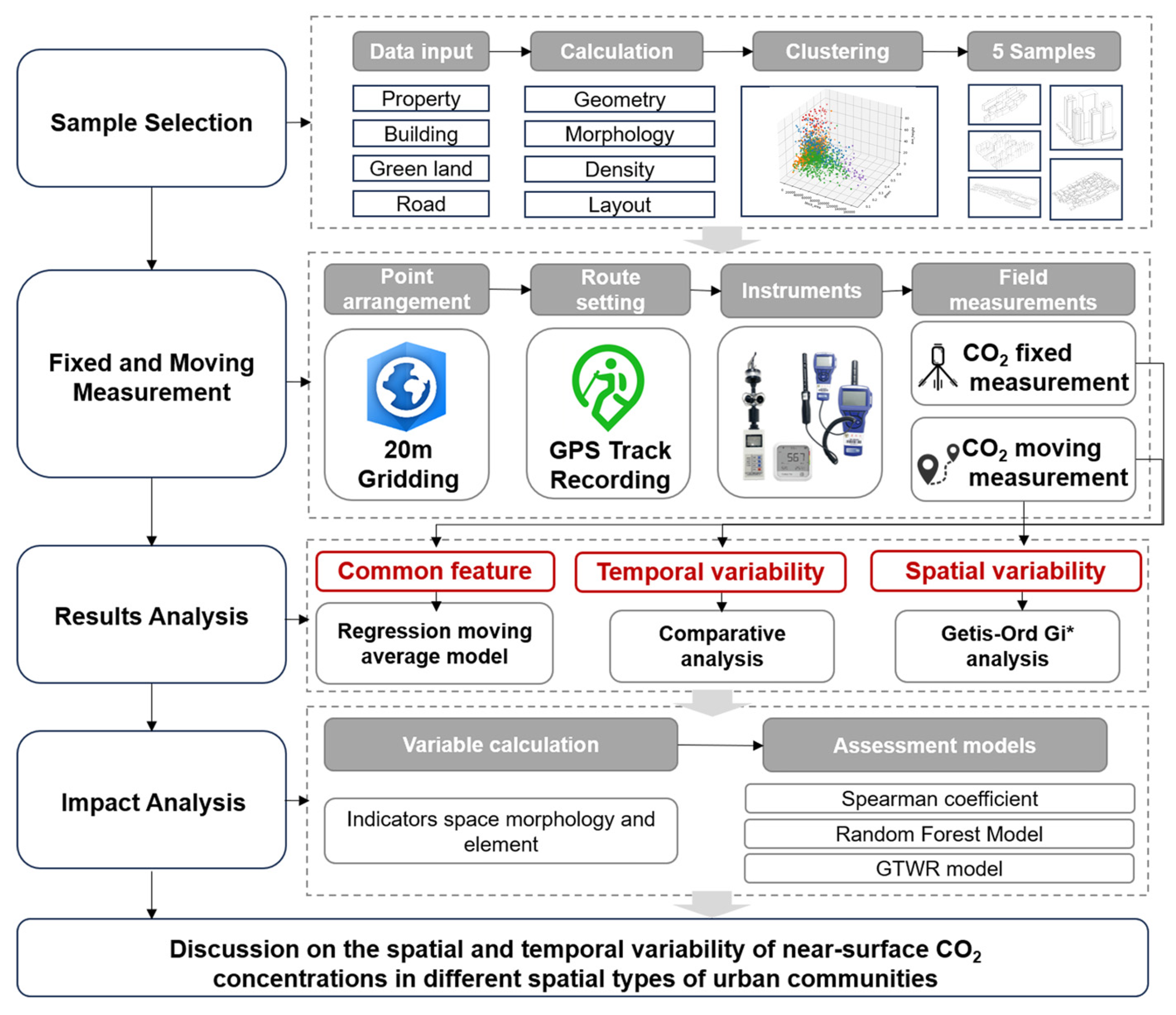
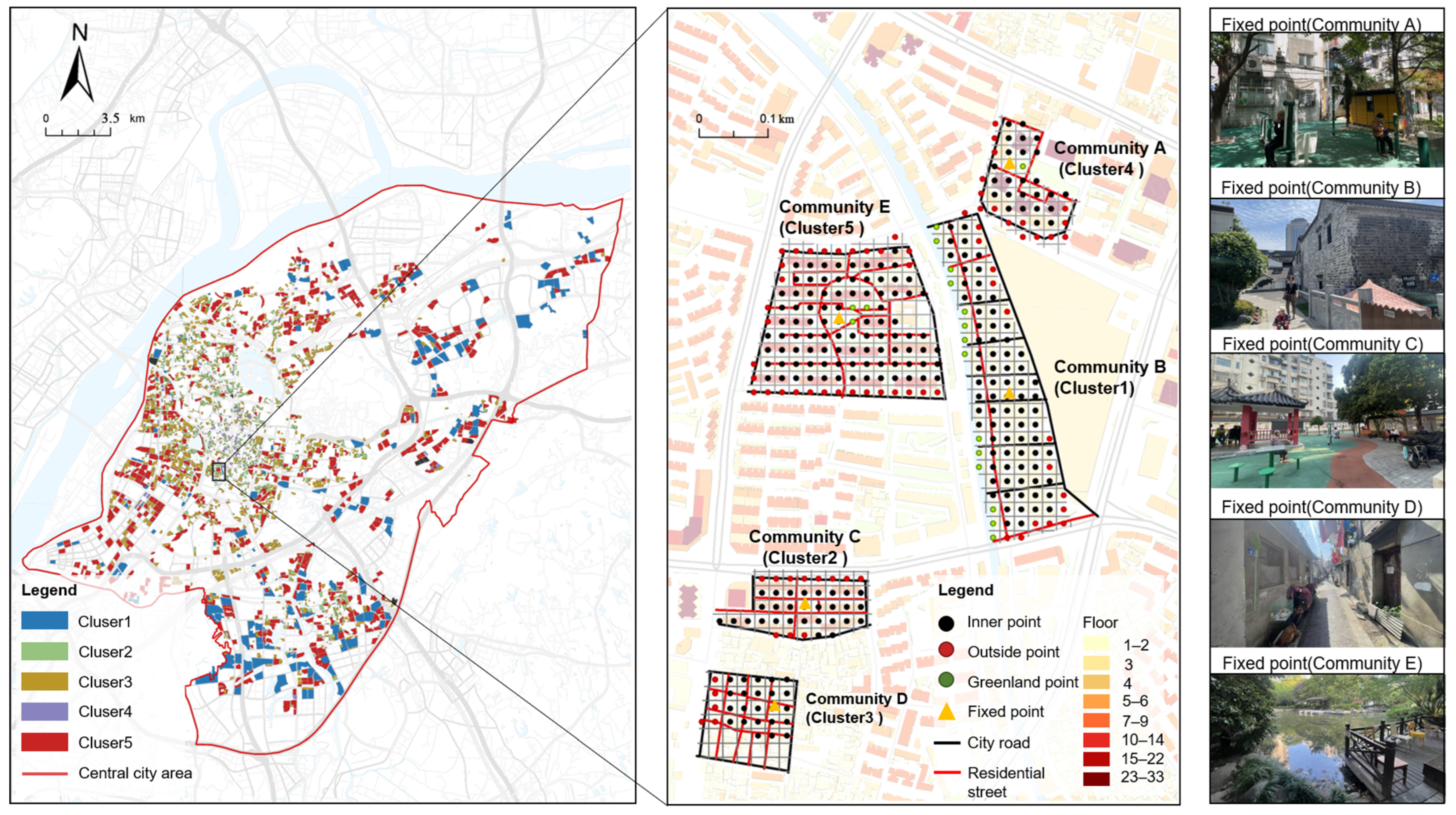
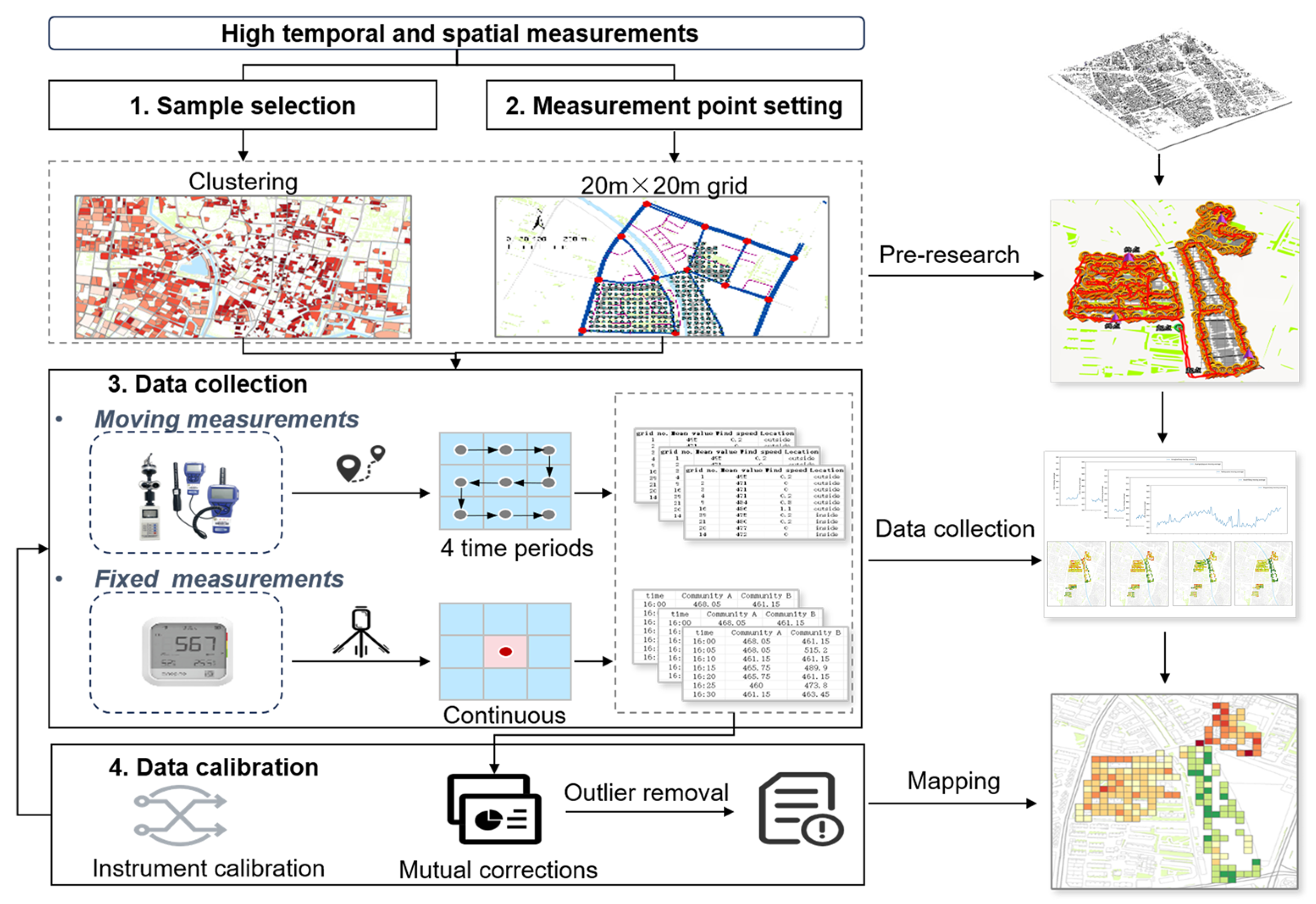
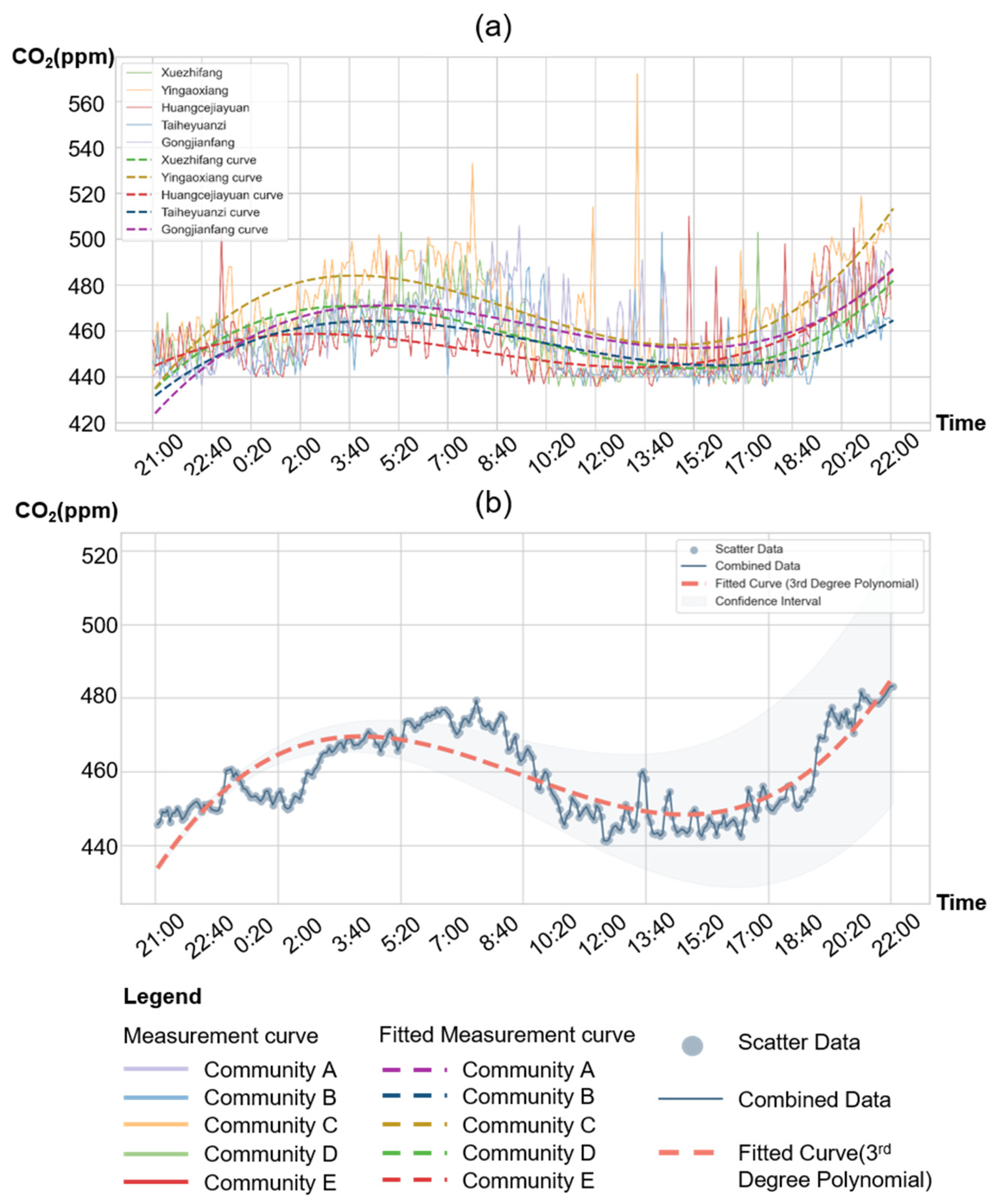
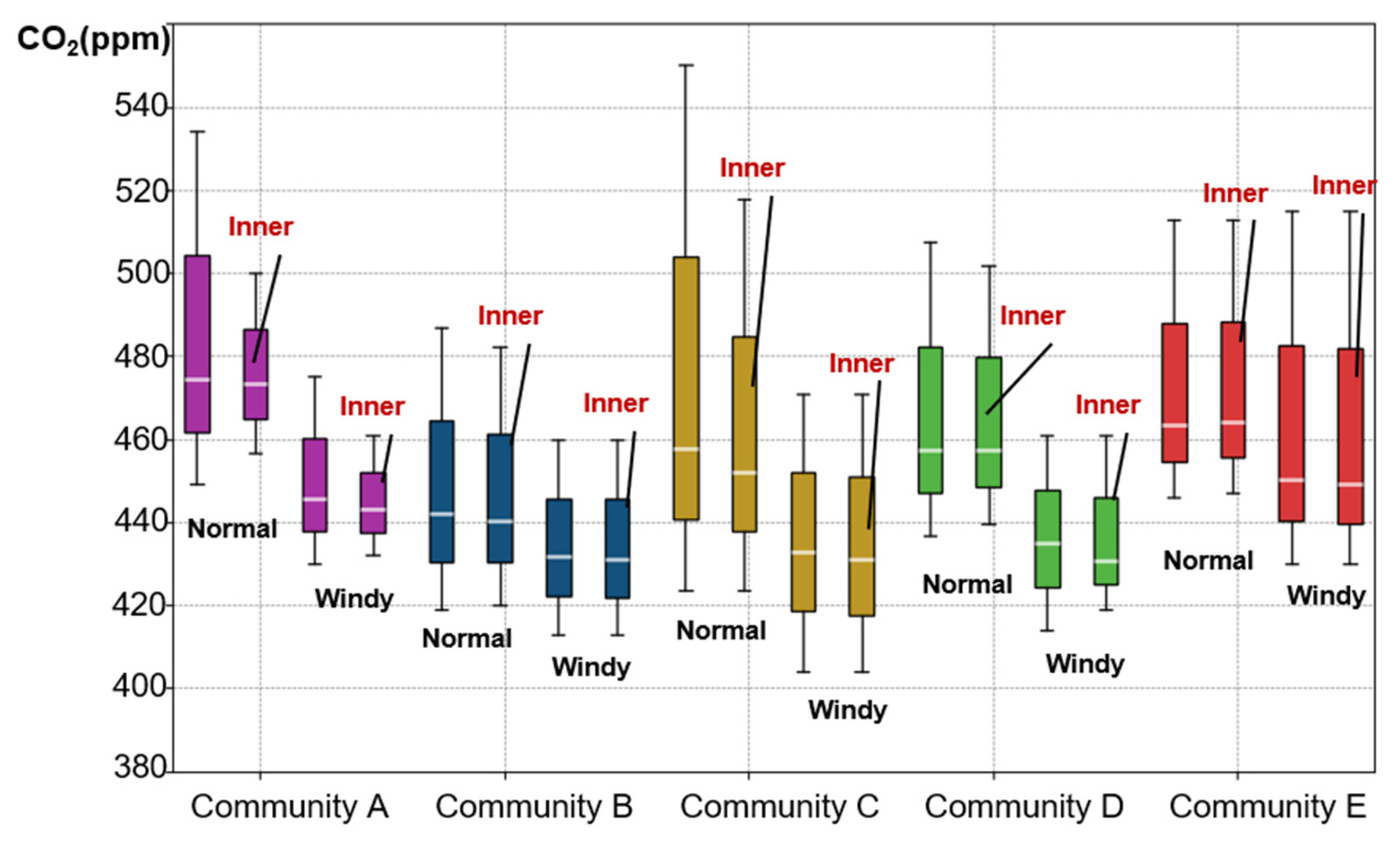
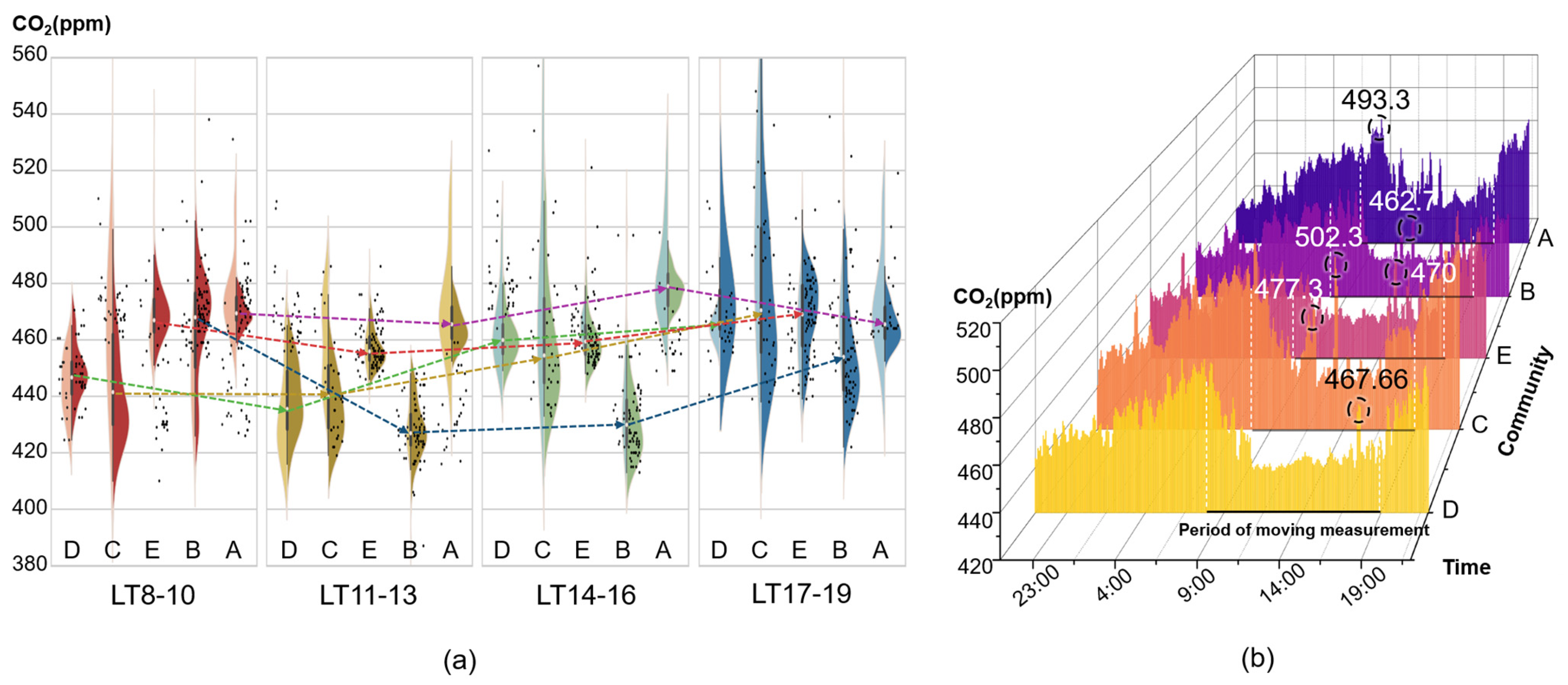


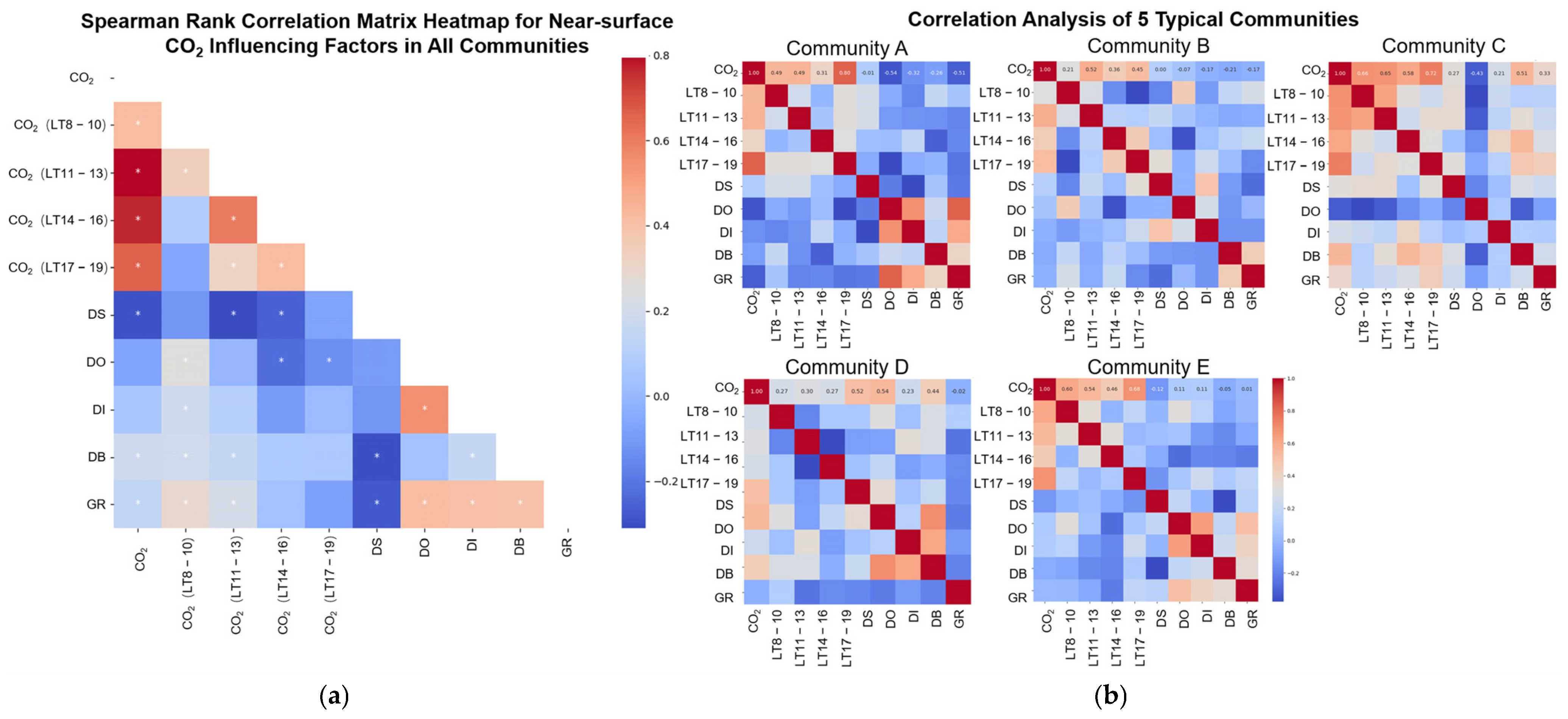
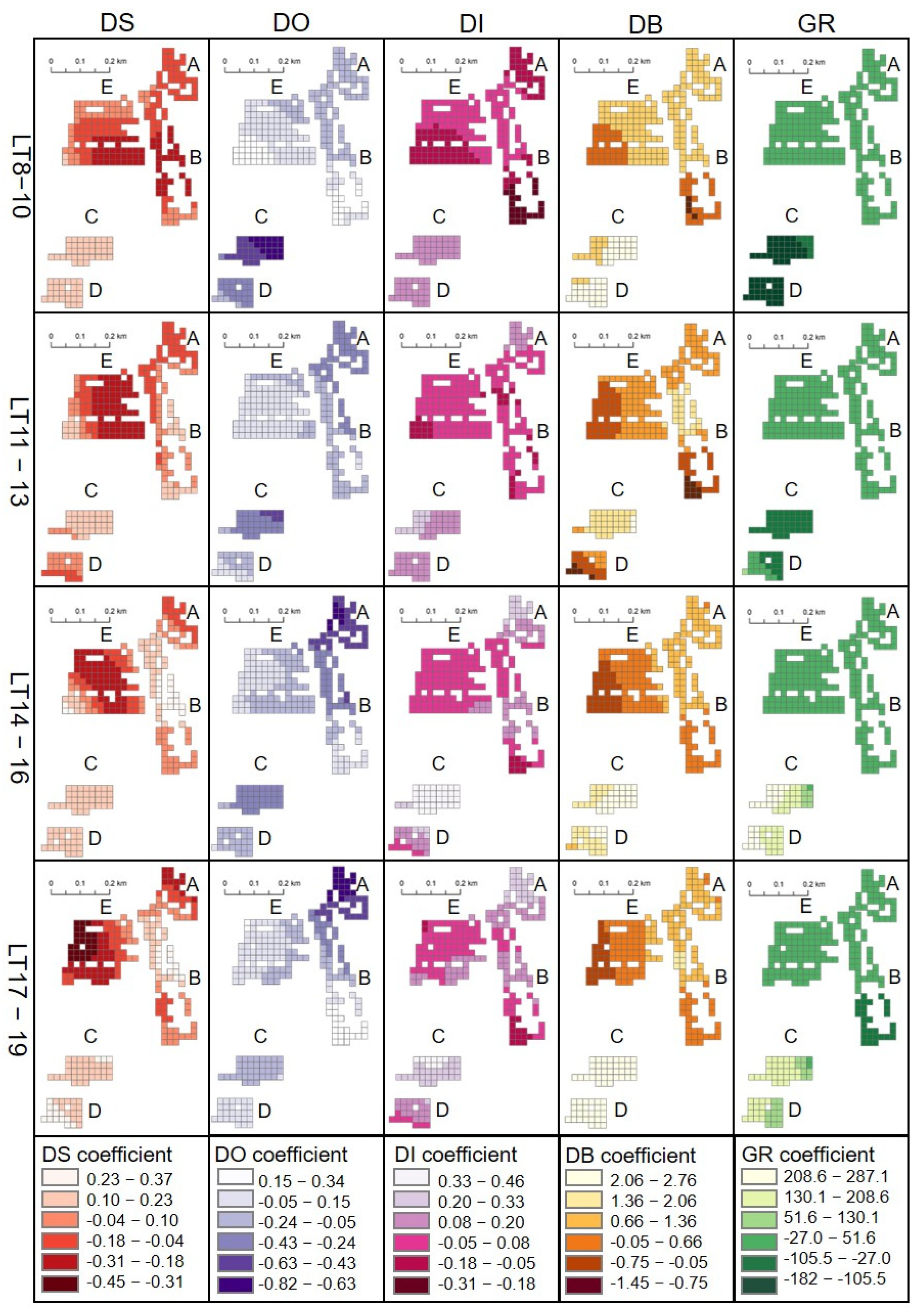
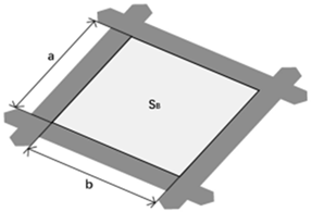
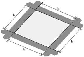
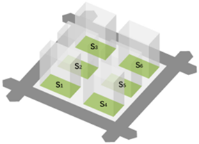
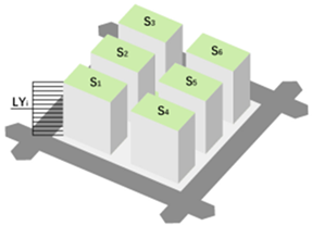
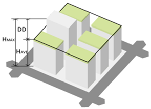
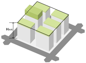
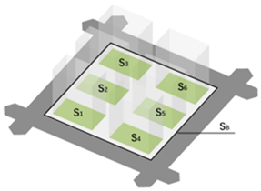
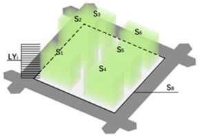
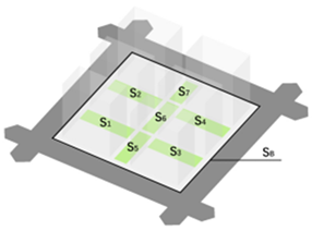
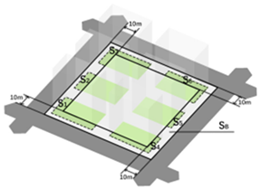
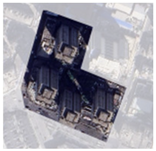
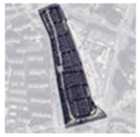
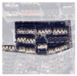
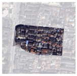
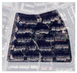
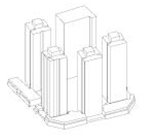

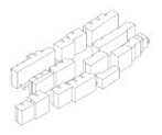
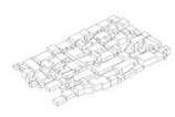

Disclaimer/Publisher’s Note: The statements, opinions and data contained in all publications are solely those of the individual author(s) and contributor(s) and not of MDPI and/or the editor(s). MDPI and/or the editor(s) disclaim responsibility for any injury to people or property resulting from any ideas, methods, instructions or products referred to in the content. |
© 2025 by the authors. Licensee MDPI, Basel, Switzerland. This article is an open access article distributed under the terms and conditions of the Creative Commons Attribution (CC BY) license (https://creativecommons.org/licenses/by/4.0/).