


Spatial Spillover Effects of Urban Gray–Green Space Form on COVID-19 Pandemic in China
 , , and
Abstract
:1. Introduction
2. Materials and Methods
2.1. Standard Deviational Ellipse Model
2.2. STIRPAT Model and Multiple Variable Regression
2.3. Spatial Econometric Model
2.4. Variables and Data Source
2.4.1. COVID-19 Infection Rate
2.4.2. Baidu Migration Scale Index
2.4.3. Quantifying Spatial Patterns
2.4.4. Urban Functional Mixing Degree
2.5. Data Resource
3. Results and Discussion
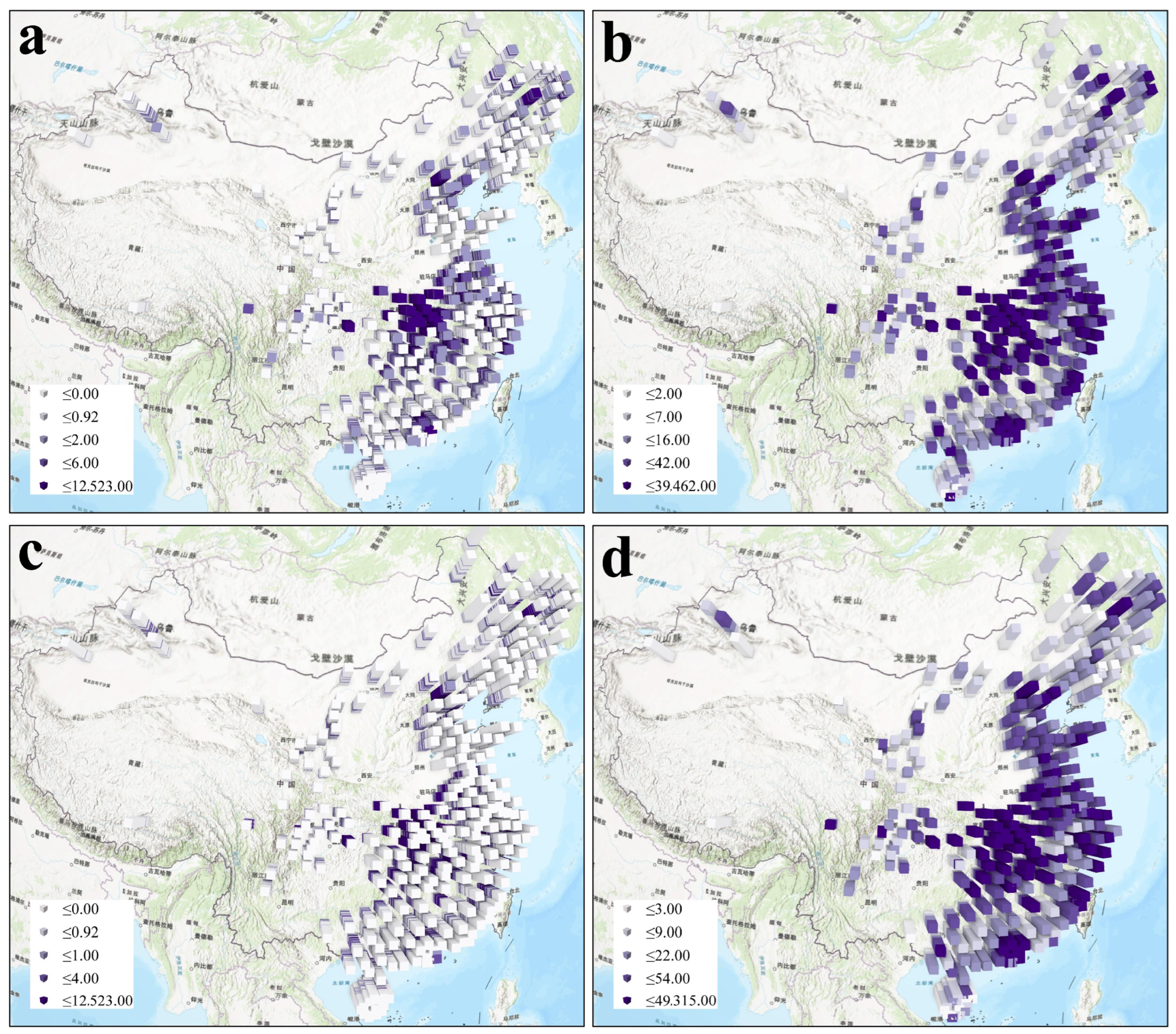
3.1. Population Mitigation, Habitat Quality, and Urban Land Use Mixture
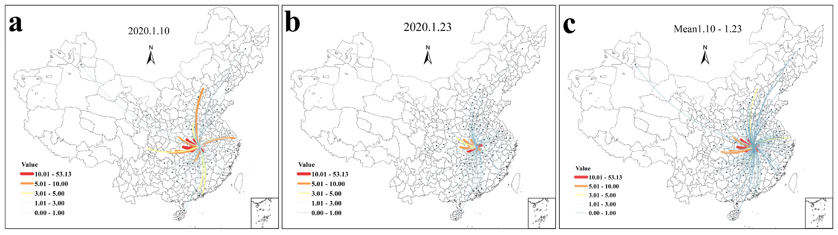
3.2. Dynamics of COVID-19 During Initial Period in China
3.3. Basic Multiple Variables Regression Results
3.4. Spatial Spillover Effects of Pandemic and Gray–Green Space Form
4. Policy Recommendation
5. Conclusions
Author Contributions
Funding
Data Availability Statement
Conflicts of Interest
References
- Elavarasan, R.M.; Pugazhendhi, R.; Shafiullah, G.; Irfan, M.; Anvari-Moghaddam, A. A hover view over effectual approaches on pandemic management for sustainable cities–the endowment of prospective technologies with revitalization strategies. Sustain. Cities Soc. 2021, 68, 102789. [Google Scholar] [CrossRef] [PubMed]
- Bourouiba, L. Fluid dynamics of respiratory infectious diseases. Annu. Rev. Biomed. Eng. 2021, 23, 547–577. [Google Scholar] [CrossRef] [PubMed]
- Afrin, S.; Chowdhury, F.J.; Rahman, M.M. COVID-19 pandemic: Rethinking strategies for resilient urban design, perceptions, and planning. Front. Sustain. Cities 2021, 3, 668263. [Google Scholar] [CrossRef]
- Honey-Rosés, J.; Anguelovski, I.; Chireh, V.K.; Daher, C.; Konijnendijk van den Bosch, C.; Litt, J.S.; Mawani, V.; McCall, M.K.; Orellana, A.; Oscilowicz, E. The impact of COVID-19 on public space: An early review of the emerging questions–design, perceptions and inequities. Cities Health 2021, 5, S263–S279. [Google Scholar] [CrossRef]
- Elliott, P.; Wartenberg, D. Spatial epidemiology: Current approaches and future challenges. Environ. Health Perspect. 2004, 112, 998–1006. [Google Scholar] [CrossRef]
- Fu, K.-Y.; Liu, Y.-Z.; Lu, X.-Y.; Chen, B.; Chen, Y.-H. Health impacts of climate resilient city development: Evidence from China. Sustain. Cities Soc. 2024, 116, 105914. [Google Scholar] [CrossRef]
- Li, A.; Mansour, A.; Bentley, R. Green and blue spaces, COVID-19 lockdowns, and mental health: An Australian population-based longitudinal analysis. Health Place 2023, 83, 103103. [Google Scholar] [CrossRef]
- Xu, Y.; Guo, C.; Yang, J.; Yuan, Z.; Ho, H.C. Modelling impact of high-rise, high-density built environment on COVID-19 risks: Empirical results from a case study of two Chinese cities. Int. J. Environ. Res. Public Health 2023, 20, 1422. [Google Scholar] [CrossRef]
- Bibri, S.E.; Krogstie, J.; Kärrholm, M. Compact city planning and development: Emerging practices and strategies for achieving the goals of sustainability. Dev. Built Environ. 2020, 4, 100021. [Google Scholar] [CrossRef]
- Kontis, V.; Bennett, J.E.; Rashid, T.; Parks, R.M.; Pearson-Stuttard, J.; Guillot, M.; Asaria, P.; Zhou, B.; Battaglini, M.; Corsetti, G. Magnitude, demographics and dynamics of the effect of the first wave of the COVID-19 pandemic on all-cause mortality in 21 industrialized countries. Nat. Med. 2020, 26, 1919–1928. [Google Scholar] [CrossRef]
- Sannigrahi, S.; Pilla, F.; Basu, B.; Basu, A.S.; Molter, A. Examining the association between socio-demographic composition and COVID-19 fatalities in the European region using spatial regression approach. Sustain. Cities Soc. 2020, 62, 102418. [Google Scholar] [CrossRef] [PubMed]
- Piltch-Loeb, R.; Abramson, D.M.; Merdjanoff, A.A. Risk salience of a novel virus: US population risk perception, knowledge, and receptivity to public health interventions regarding the Zika virus prior to local transmission. PLoS ONE 2017, 12, e0188666. [Google Scholar] [CrossRef]
- Connolly, C.; Ali, S.H.; Keil, R. On the relationships between COVID-19 and extended urbanization. Dialogues Hum. Geogr. 2020, 10, 213–216. [Google Scholar] [CrossRef]
- Selden, T.M.; Berdahl, T.A. COVID-19 and racial/ethnic disparities in health risk, employment, and household composition: Study examines potential explanations for racial-ethnic disparities in COVID-19 hospitalizations and mortality. Health Aff. 2020, 39, 1624–1632. [Google Scholar] [CrossRef]
- Paital, B. Nurture to nature via COVID-19, a self-regenerating environmental strategy of environment in global context. Sci. Total Environ. 2020, 729, 139088. [Google Scholar] [CrossRef]
- Perico, L.; Tomasoni, S.; Peracchi, T.; Perna, A.; Pezzotta, A.; Remuzzi, G.; Benigni, A. COVID-19 and lombardy: TESTing the impact of the first wave of the pandemic. EBioMedicine 2020, 61, 103069. [Google Scholar] [CrossRef] [PubMed]
- Singh, R.P.; Chauhan, A. Impact of lockdown on air quality in India during COVID-19 pandemic. Air Qual. Atmos. Health 2020, 13, 921–928. [Google Scholar] [CrossRef] [PubMed]
- Altena, E.; Baglioni, C.; Espie, C.A.; Ellis, J.; Gavriloff, D.; Holzinger, B.; Schlarb, A.; Frase, L.; Jernelöv, S.; Riemann, D. Dealing with sleep problems during home confinement due to the COVID-19 outbreak: Practical recommendations from a task force of the European CBT-I Academy. J. Sleep Res. 2020, 29, e13052. [Google Scholar] [CrossRef]
- Rodríguez-Urrego, D.; Rodríguez-Urrego, L. Air quality during the COVID-19: PM2.5 analysis in the 50 most polluted capital cities in the world. Environ. Pollut. 2020, 266, 115042. [Google Scholar] [CrossRef]
- Sagripanti, J.L.; Lytle, C.D. Estimated inactivation of coronaviruses by solar radiation with special reference to COVID-19. Photochem. Photobiol. 2020, 96, 731–737. [Google Scholar] [CrossRef]
- Gibb, R.; Redding, D.W.; Chin, K.Q.; Donnelly, C.A.; Blackburn, T.M.; Newbold, T.; Jones, K.E. Zoonotic host diversity increases in human-dominated ecosystems. Nature 2020, 584, 398–402. [Google Scholar] [CrossRef]
- Newbold, T.; Hudson, L.N.; Hill, S.L.; Contu, S.; Lysenko, I.; Senior, R.A.; Börger, L.; Bennett, D.J.; Choimes, A.; Collen, B. Global effects of land use on local terrestrial biodiversity. Nature 2015, 520, 45–50. [Google Scholar] [CrossRef]
- Venter, Z.S.; Barton, D.N.; Gundersen, V.; Figari, H.; Nowell, M. Urban nature in a time of crisis: Recreational use of green space increases during the COVID-19 outbreak in Oslo, Norway. Environ. Res. Lett. 2020, 15, 104075. [Google Scholar] [CrossRef]
- Hu, Y.; Lin, Z.; Jiao, S.; Zhang, R. High-density communities and infectious disease vulnerability: A built environment perspective for sustainable health development. Buildings 2023, 14, 103. [Google Scholar] [CrossRef]
- Kelly, M.R., Jr.; Tien, J.H.; Eisenberg, M.C.; Lenhart, S. The impact of spatial arrangements on epidemic disease dynamics and intervention strategies. J. Biol. Dyn. 2016, 10, 222–249. [Google Scholar] [CrossRef]
- Rader, B.; Scarpino, S.V.; Nande, A.; Hill, A.L.; Adlam, B.; Reiner, R.C.; Pigott, D.M.; Gutierrez, B.; Zarebski, A.E.; Shrestha, M. Crowding and the shape of COVID-19 epidemics. Nat. Med. 2020, 26, 1829–1834. [Google Scholar] [CrossRef]
- Liu, C.; Liu, Z.; Guan, C. The impacts of the built environment on the incidence rate of COVID-19: A case study of King County, Washington. Sustain. Cities Soc. 2021, 74, 103144. [Google Scholar] [CrossRef]
- Wu, Y.; Wei, Y.D.; Liu, M.; García, I. Green infrastructure inequality in the context of COVID-19: Taking parks and trails as examples. Urban For. Urban Green. 2023, 86, 128027. [Google Scholar] [CrossRef]
- Berdejo-Espinola, V.; Suárez-Castro, A.F.; Amano, T.; Fielding, K.S.; Oh, R.R.Y.; Fuller, R.A. Urban green space use during a time of stress: A case study during the COVID-19 pandemic in Brisbane, Australia. People Nat. 2021, 3, 597–609. [Google Scholar] [CrossRef]
- Bowler, D.E.; Buyung-Ali, L.; Knight, T.M.; Pullin, A.S. Urban greening to cool towns and cities: A systematic review of the empirical evidence. Landsc. Urban Plan. 2010, 97, 147–155. [Google Scholar] [CrossRef]
- Kleinschroth, F.; Kowarik, I. COVID-19 crisis demonstrates the urgent need for urban greenspaces. Front. Ecol. Environ. 2020, 18, 318. [Google Scholar] [CrossRef]
- Liu, S.; Wang, X. Reexamine the value of urban pocket parks under the impact of the COVID-19. Urban For. Urban Green. 2021, 64, 127294. [Google Scholar] [CrossRef]
- You, Y.; Pan, S. Urban vegetation slows down the spread of coronavirus disease (COVID-19) in the United States. Geophys. Res. Lett. 2020, 47, e2020GL089286. [Google Scholar] [CrossRef]
- Gallotti, R.; Sacco, P.; De Domenico, M. Complex urban systems: Challenges and integrated solutions for the sustainability and resilience of cities. Complexity 2021, 2021, 1782354. [Google Scholar] [CrossRef]
- Pickett, S.; Cadenasso, M.; Rosi-Marshall, E.J.; Belt, K.T.; Groffman, P.M.; Grove, J.M.; Irwin, E.G.; Kaushal, S.S.; LaDeau, S.L.; Nilon, C.H. Dynamic heterogeneity: A framework to promote ecological integration and hypothesis generation in urban systems. Urban Ecosyst. 2017, 20, 1–14. [Google Scholar] [CrossRef]
- Nelson, K.S.; Nguyen, T.D.; Brownstein, N.A.; Garcia, D.; Walker, H.C.; Watson, J.T.; Xin, A. Definitions, measures, and uses of rurality: A systematic review of the empirical and quantitative literature. J. Rural. Stud. 2021, 82, 351–365. [Google Scholar] [CrossRef]
- Zhu, Z.; Qiu, S.; Ye, S. Remote sensing of land change: A multifaceted perspective. Remote Sens. Environ. 2022, 282, 113266. [Google Scholar] [CrossRef]
- Polyak, B.T.; Nazin, S.A.; Durieu, C.; Walter, E. Ellipsoidal parameter or state estimation under model uncertainty. Automatica 2004, 40, 1171–1179. [Google Scholar] [CrossRef]
- Nevitt, J.; Hancock, G.R. Performance of bootstrapping approaches to model test statistics and parameter standard error estimation in structural equation modeling. Struct. Equ. Model. 2001, 8, 353–377. [Google Scholar] [CrossRef]
- Fischer-Kowalski, M.; Amann, C. Beyond IPAT and Kuznets curves: Globalization as a vital factor in analysing the environmental impact of socio-economic metabolism. Popul. Environ. 2001, 23, 7–47. [Google Scholar] [CrossRef]
- Dietz, T.; Rosa, E.A. Effects of population and affluence on CO2 emissions. Proc. Natl. Acad. Sci. USA 1997, 94, 175–179. [Google Scholar] [CrossRef]
- Shahbaz, M.; Loganathan, N.; Muzaffar, A.T.; Ahmed, K.; Jabran, M.A. How urbanization affects CO2 emissions in Malaysia? The application of STIRPAT model. Renew. Sustain. Energy Rev. 2016, 57, 83–93. [Google Scholar] [CrossRef]
- Dietz, T.; Rosa, E.A. Rethinking the environmental impacts of population, affluence and technology. Hum. Ecol. Rev. 1994, 1, 277–300. [Google Scholar]
- Arenas, A.; Cota, W.; Gómez-Gardeñes, J.; Gómez, S.; Granell, C.; Matamalas, J.T.; Soriano-Paños, D.; Steinegger, B. Modeling the spatiotemporal epidemic spreading of COVID-19 and the impact of mobility and social distancing interventions. Phys. Rev. X 2020, 10, 041055. [Google Scholar] [CrossRef]
- Ostergaard, L. SARS CoV-2 related microvascular damage and symptoms during and after COVID-19: Consequences of capillary transit-time changes, tissue hypoxia and inflammation. Physiol. Rep. 2021, 9, e14726. [Google Scholar] [CrossRef]
- Liu, Y.; Wang, Z.; Rader, B.; Li, B.; Wu, C.-H.; Whittington, J.D.; Zheng, P.; Stenseth, N.C.; Bjornstad, O.N.; Brownstein, J.S. Associations between changes in population mobility in response to the COVID-19 pandemic and socioeconomic factors at the city level in China and country level worldwide: A retrospective, observational study. Lancet Digit. Health 2021, 3, e349–e359. [Google Scholar] [CrossRef]
- Hamidi, S.; Sabouri, S.; Ewing, R. Does density aggravate the COVID-19 pandemic? Early findings and lessons for planners. J. Am. Plan. Assoc. 2020, 86, 495–509. [Google Scholar] [CrossRef]
- Sun, Z.; Zhang, H.; Yang, Y.; Wan, H.; Wang, Y. Impacts of geographic factors and population density on the COVID-19 spreading under the lockdown policies of China. Sci. Total Environ. 2020, 746, 141347. [Google Scholar] [CrossRef]
- Gupta, S.; Nguyen, T.; Raman, S.; Lee, B.; Lozano-Rojas, F.; Bento, A.; Simon, K.; Wing, C. Tracking public and private responses to the COVID-19 epidemic: Evidence from state and local government actions. Am. J. Health Econ. 2021, 7, 361–404. [Google Scholar] [CrossRef]
- Frieden, T.R.; Lee, C.T. Identifying and interrupting superspreading events—Implications for control of severe acute respiratory syndrome coronavirus 2. Emerg. Infect. Dis. 2020, 26, 1059. [Google Scholar] [CrossRef]
- Gaskin, D.J.; Zare, H.; Delarmente, B.A. Geographic disparities in COVID-19 infections and deaths: The role of transportation. Transp. Policy 2021, 102, 35–46. [Google Scholar] [CrossRef] [PubMed]
- Ebrahimi, O.V.; Hoffart, A.; Johnson, S.U. Viral mitigation and the COVID-19 pandemic: Factors associated with adherence to social distancing protocols and hygienic behaviour. Psychol. Health 2023, 38, 283–306. [Google Scholar] [CrossRef]
- Coccia, M. How do low wind speeds and high levels of air pollution support the spread of COVID-19? Atmos. Pollut. Res. 2021, 12, 437–445. [Google Scholar] [CrossRef] [PubMed]
- Ju, M.J.; Oh, J.; Choi, Y.-H. Changes in air pollution levels after COVID-19 outbreak in Korea. Sci. Total Environ. 2021, 750, 141521. [Google Scholar] [CrossRef]
- Moreira, D.N.; Da Costa, M.P. The impact of the Covid-19 pandemic in the precipitation of intimate partner violence. Int. J. Law Psychiatry 2020, 71, 101606. [Google Scholar] [CrossRef]
- Notari, A. Temperature dependence of COVID-19 transmission. Sci. Total Environ. 2021, 763, 144390. [Google Scholar] [CrossRef] [PubMed]
- Hsiao, W.-S.; Huang, S.-Y. Fostering small urban green spaces: Public–private partnerships as a synergistic approach to forming new public life in Taipei City. Urban For. Urban Green. 2024, 91, 128169. [Google Scholar] [CrossRef]
- Li, Q.; Bessell, L.; Xiao, X.; Fan, C.; Gao, X.; Mostafavi, A. Disparate patterns of movements and visits to points of interest located in urban hotspots across US metropolitan cities during COVID-19. R. Soc. Open Sci. 2021, 8, 201209. [Google Scholar] [CrossRef]
- Spagnolello, O.; Rota, S.; Valoti, O.F.; Cozzini, C.; Parrino, P.; Portella, G.; Langer, M. Bergamo field hospital confronting COVID-19: Operating instructions. Disaster Med. Public Health Prep. 2022, 16, 875–877. [Google Scholar] [CrossRef]
- Ward, M.D.; Gleditsch, K.S. Spatial Regression Models; Sage Publications: Thousand Oaks, CA, USA, 2018; Volume 2018. [Google Scholar]
- Caldas, M.; Walker, R.; Arima, E.; Perz, S.; Aldrich, S.; Simmons, C. Theorizing land cover and land use change: The peasant economy of Amazonian deforestation. Ann. Am. Assoc. Geogr. 2007, 97, 86–110. [Google Scholar] [CrossRef]
- Khavarian-Garmsir, A.R.; Pourahmad, A.; Hataminejad, H.; Farhoodi, R. Climate change and environmental degradation and the drivers of migration in the context of shrinking cities: A case study of Khuzestan province, Iran. Sustain. Cities Soc. 2019, 47, 101480. [Google Scholar] [CrossRef]
- Huang, J.; Lu, X.X.; Sellers, J.M. A global comparative analysis of urban form: Applying spatial metrics and remote sensing. Landsc. Urban Plan. 2007, 82, 184–197. [Google Scholar] [CrossRef]
- Jia, Y.; Tang, L.; Xu, M.; Yang, X. Landscape pattern indices for evaluating urban spatial form–A case study of Chinese cities. Ecol. Indic. 2019, 99, 27–37. [Google Scholar] [CrossRef]
- Liu, X.; Li, X.; Chen, Y.; Tan, Z.; Li, S.; Ai, B. A new landscape index for quantifying urban expansion using multi-temporal remotely sensed data. Landsc. Ecol. 2010, 25, 671–682. [Google Scholar] [CrossRef]
- Li, Z.; Wang, F.; Kang, T.T.; Wang, C.J.; Chen, X.D.; Miao, Z.; Zhang, L.; Ye, Y.Y.; Zhang, H.O. Exploring differentiated impacts of socioeconomic factors and urban forms on city-level CO2 emissions in China: Spatial heterogeneity and varying importance levels. Sustain. Cities Soc. 2022, 84, 104028. [Google Scholar] [CrossRef]
- Abdi, H.; Williams, L.J. Principal component analysis. Wiley Interdiscip. Rev. Comput. Stat. 2010, 2, 433–459. [Google Scholar] [CrossRef]
- Hu, S.; He, Z.; Wu, L.; Yin, L.; Xu, Y.; Cui, H. A framework for extracting urban functional regions based on multiprototype word embeddings using points-of-interest data. Comput. Environ. Urban Syst. 2020, 80, 101442. [Google Scholar] [CrossRef]
- Zhang, Y.; Yang, Z.; Li, W. Analyses of urban ecosystem based on information entropy. Ecol. Model. 2006, 197, 1–12. [Google Scholar] [CrossRef]
- Anselin, L.; Le Gallo, J.; Jayet, H. Spatial panel econometrics. In The Econometrics of Panel Data, Fundamentals and Recent Developments in Theory and Practice; Springer: Berlin/Heidelberg, Germany, 2008. [Google Scholar]
- Hazarie, S.; Soriano-Paños, D.; Arenas, A.; Gómez-Gardeñes, J.; Ghoshal, G. Interplay between population density and mobility in determining the spread of epidemics in cities. Commun. Phys. 2021, 4, 191. [Google Scholar] [CrossRef]
- Zhang, M.; Wang, S.; Hu, T.; Fu, X.; Wang, X.; Hu, Y.; Halloran, B.; Li, Z.; Cui, Y.; Liu, H. Human mobility and COVID-19 transmission: A systematic review and future directions. Ann. GIS 2022, 28, 501–514. [Google Scholar] [CrossRef]
- Pan, J.; Bardhan, R.; Jin, Y. Spatial distributive effects of public green space and COVID-19 infection in London. Urban For. Urban Green. 2021, 62, 127182. [Google Scholar] [CrossRef] [PubMed]
- Yin, H.; Sun, T.; Yao, L.; Jiao, Y.; Ma, L.; Lin, L.; Graff, J.C.; Aleya, L.; Postlethwaite, A.; Gu, W.; et al. Association between population density and infection rate suggests the importance of social distancing and travel restriction in reducing the COVID-19 pandemic. Environ. Sci. Pollut. Res. 2021, 28, 40424–40430. [Google Scholar] [CrossRef] [PubMed]
- Abozeid, A.S.M.; AboElatta, T.A. Polycentric vs monocentric urban structure contribution to national development. J. Eng. Appl. Sci. 2021, 68, 11. [Google Scholar] [CrossRef]
- Liu, L.; Zhong, Y.; Ao, S.; Wu, H. Exploring the relevance of green space and epidemic diseases based on panel data in China from 2007 to 2016. Int. J. Environ. Res. Public Health 2019, 16, 2551. [Google Scholar] [CrossRef] [PubMed]
- Poortinga, W.; Bird, N.; Hallingberg, B.; Phillips, R.; Williams, D. The role of perceived public and private green space in subjective health and wellbeing during and after the first peak of the COVID-19 outbreak. Landsc. Urban Plan. 2021, 211, 104092. [Google Scholar] [CrossRef]


| Dimension | Variable | Selection Basis |
|---|---|---|
| Socio- economic | Wuhan migration outflow scale index | Studies from a demographic perspective have focused on the impact of population mobility on the spread of the epidemic, and it is generally recognized that population mobility accelerates the spread of the epidemic and that the outflow of people from Wuhan is the most important factor influencing the number of cases in each location. Accordingly, the Wuhan city lockdown to limit the population was key to the rapid and effective control of the epidemic [44,46]. |
| Inter-city migration intensity | ||
| Intra-city travel intensity | ||
| Population density | Several studies have shown that COVID-19 spreads more rapidly in areas with high population densities than in areas with low population densities [47,48]. | |
| Public budget expenditure | Local government expenditures on various activities in the region can reflect the efforts of local governments in responding to the spread of COVID-19 [49]. | |
| Number of hospital beds | It reflects the level of local medical conditions. Timely admission for treatment and the isolation of cases will reduce the probability of spreading the epidemic [50]. | |
| Road density | It reflects traffic road transportation. Average distance traveled and commuting distance may be associated with higher incidence of COVID-19 transmission, and reduced travel during an outbreak is important in delaying outbreaks [51]. | |
| Education level | The higher the level of education of the people, the greater the awareness of self-protection and the conscientious implementation of the quarantine policy, which is conducive to the implementation of policies formulated by the government and the control of the spread of the epidemic [52]. | |
| Ecological environment | Daily average temperature | Studies have shown that ecological environment and climatic conditions, as the main ways and influencing factors of virus transmission and population infection, play an important role in the occurrence, development, spread, prevention, and control of the epidemic. Temperature, wind speed, rainfall, and air particulate matter concentration play an important role in the spread of the virus [53]. Low temperature, low humidity, and a high concentration of air particulate matter exposure are more conducive to the spread of coronavirus in the environment [54]. Air pollution such as inhalable fine particulate matter (PM2.5) is an important risk factor for the COVID-19 epidemic [55,56]. |
| Precipitation | ||
| Wind speed | ||
| Air pollution level | ||
| Urban Form | Patch size | In most cases, green area and green rate are used to quantify landscape features, while their spatial configuration is ignored. However, more complex and fragmented landscapes are associated with more ecological processes, which increases the possibility of contact with various infectious diseases [57]. As urbanization has accelerated the exchange of people, the compression of space has provided a hotbed for the spread of the epidemic and enhanced the ability of the virus to spread. The urban gray building and ecological green space form a way of integration and blocking [58]. The gray–green space can control the source of infection, block the route of transmission, and protect the susceptible population directly or indirectly by affecting the atmospheric environment and controlling human behavior, and prevent the spread of the epidemic by inhibiting the epidemic conditions of infectious diseases [45]. At the same time, gray–green space can affect the climate through ecological effects, and can greatly affect the spread of urban COVID-19 by providing ecosystem services and as an urban disaster shelter [59]. The composition and degree of mixing within urban functional areas significantly influence the spread of the COVID-19 virus. |
| Patch polycentricity | ||
| Patch shape | ||
| Patch fragmentation | ||
| Patch connectivity | ||
| Patch compactness | ||
| Patch sprawl | ||
| Urban functional mixing degree |
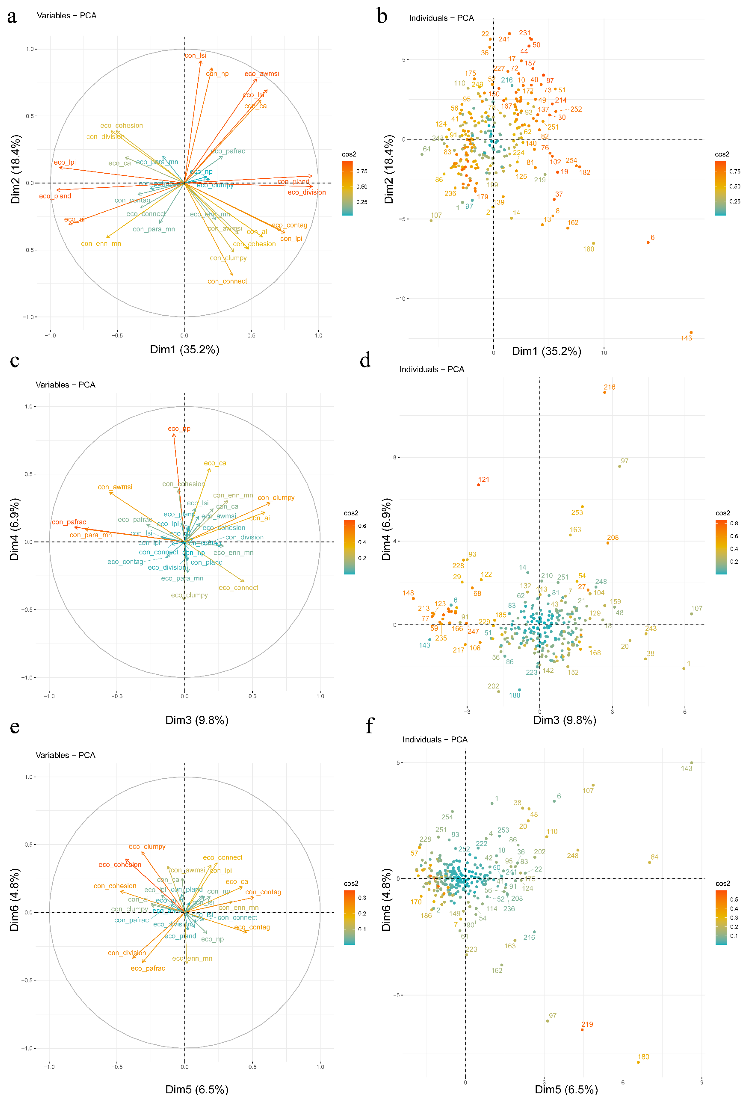
| Principal Component | Spatial Pattern Indicators | Cumulative |
|---|---|---|
| pc1 | Gray space scale and monocentricity | 0.352 |
| pc2 | Gray space shape complexity and fragmentation | 0.536 |
| pc3 | Gray space compactness | 0.634 |
| pc4 | Green space fragmentation and scale | 0.709 |
| pc5 | Green space connectivity | 0.774 |
| pc6 | Green space compactness | 0.822 |
| Dimension | Variable Name | Symbol | Description | Unit |
|---|---|---|---|---|
| Socio- economic | COVID-19 incidence rate | Covi | Confirmed cases/City’s annual average population in the specified time period | % |
| Wuhan migration outflow scale index | lnwhq | Population outflow before Wuhan lockdown | / | |
| Inter-city migration intensity | lnimin | Inter-city population migration volume | / | |
| Intra-city travel intensity | lnicin | Intra-city travel intensity | / | |
| Population density | lnpopd | Permanent population/Administrative area of the city | cases/km2 | |
| Public budget expenditure | lnpbe | Local government expenditure on various activities in the region | 10,000 RMB | |
| Number of hospital beds | lnnhb | Number of hospital beds in the city | number | |
| Road density | lnroads | Total road length/Administrative area of the city | km/km2 | |
| Education level | lnedu | City’s expenditure on the education sector | 10,000 RMB | |
| Ecological environment | Daily average temperature | lntem | Average temperature during the specified time period | ℃ |
| Precipitation | lnpre | Average precipitation during the specified time period | mm3 | |
| Wind speed | lnwind | Average wind speed during the specified time period | m/s | |
| Air pollution level | lnPM2.5 | Average PM2.5 concentration during the specified time period | μg/m3 | |
| Spatial form | Gray space scale and monocentricity | pc1 | Indicator derived from principal component analysis | / |
| Gray space shape complexity and fragmentation | pc2 | Indicator derived from principal component analysis | / | |
| Gray space compactness | pc3 | Indicator derived from principal component analysis | / | |
| Green space fragmentation and scale | pc4 | Indicator derived from principal component analysis | / | |
| Green space connectivity | pc5 | Indicator derived from principal component analysis | / | |
| Green space compactness | pc6 | Indicator derived from principal component analysis | / | |
| entroy | lnentroy | Urban functional mixing degree | / |
| Variables | Standardized Coefficient (Beta) | T | Significance | VIF |
|---|---|---|---|---|
| (Constants) | 0.121 | 0.357 | 0.721 | 1.256 |
| lnwhq | 0.779 | 14.102 | 0 | 2.666 |
| lnimin | 0.175 | −1.979 | 0.249 | 16.42 |
| lnicin | 0.102 | −2.347 | 0.02 | 1.662 |
| lnpopd | 0.002 | 0.044 | 0.965 | 1.185 |
| lnpbe | −0.395 | 2.237 | 0.026 | 4.231 |
| lnnhb | 0.048 | 0.456 | 0.649 | 15.26 |
| lnedu | −0.256 | −1.384 | 0.068 | 3.954 |
| lnroads | 0.003 | 0.052 | 0.959 | 3.4 |
| lntem | 0.046 | 0.553 | 0.581 | 6.025 |
| lnpro | −0.071 | 1.655 | 0.099 | 1.627 |
| lnwind | 0.004 | −0.092 | 0.927 | 1.536 |
| lnPM2.5 | 0.088 | −1.253 | 0.012 | 4.274 |
| pc1 | 0.007 | 0.092 | 0.926 | 4.348 |
| pc2 | 0.042 | 0.762 | 0.447 | 2.636 |
| pc3 | 0.01 | 0.208 | 0.835 | 1.997 |
| pc4 | −0.038 | −0.822 | 0.412 | 1.818 |
| pc5 | −0.018 | −0.446 | 0.056 | 1.437 |
| pc6 | 0.104 | 2.349 | 0.22 | 1.708 |
| lnentroy | −0.006 | −0.164 | 0.87 | 1.32 |
| adj_R2 | 0.62 |
| Test Methods | Z Statistics | p Values |
|---|---|---|
| LM-lag | 25.36 *** | 0.001 |
| Robust-LM-lag | 112.32 *** | 0.001 |
| LM-error | 253.62 *** | 0.000 |
| Robust-LM-error | 389.56 *** | 0.000 |
| Wald-spatial-lag | 22.36 *** | 0.002 |
| Wald-spatial-error | 19.56 *** | 0.001 |
| LR-spatial-lag | 21.96 ** | 0.001 |
| LR-spatial-error | 20.69 ** | 0.002 |
| Hausman | 56.23 ** | 0.001 |
| Variable | Coefficient | p Value | Variable | W∙Coefficient | p Value |
|---|---|---|---|---|---|
| Constant | −3.62 | 0.19 | |||
| lnwhq | 1.49 | 0.00 *** | W∙Lnwhq | 0.47 | 0.00 |
| lnicin | 0.42 | 0.02 ** | W∙Lncncx | 0.21 | 0.01 |
| lnpopd | 0.05 | 0.58 | W Lnpopd | −2.37 | 0.12 |
| lnpbe | −0.73 | 0.04 ** | W * Lndfzc | 1.50 | 0.81 |
| lnedu | −0.15 | 0.64 | W * Lnedu | −0.25 | 0.97 |
| lnroads | 0.23 | 0.15 | W * Lnroads | −5.70 | 0.11 |
| lnpre | −0.02 | 0.59 | W * Lnpro | −0.53 | 0.11 |
| lntem | 0.08 | 0.01 *** | W * Lntem | 0.03 | 0.15 |
| lnwind | 0.19 | 0.55 | W * Lnwind | −3.68 | 0.57 |
| lnPM2.5 | 0.05 | 0.01 *** | W∙Lnpm2.5 | 0.08 | 0.03 |
| pc1 | 0.04 | 0.27 | W∙pc1 | 0.06 | 0.02 |
| pc2 | −0.01 | 0.89 | W∙pc2 | −0.62 | 0.27 |
| pc3 | −0.02 | 0.7 | W∙pc3 | 0.43 | 0.55 |
| pc4 | −0.04 | 0.4 | W∙pc4 | 0.28 | 0.80 |
| pc5 | −0.07 | 0.03 ** | W∙pc5 | −0.12 | 0.04 |
| pc6 | 0.03 | 0.62 | W∙pc6 | 2.48 | 0.16 |
| lnentroy | 0.28 | 0.50 | W∙lnentroy | 1.37 | 0.36 |
| ρ | 0.45 | p < 0.05 | |||
| R2 | 0.76 | p < 0.01 | |||
| Hausman | 20.12 | p < 0.01 | |||
| LR_SLM | 125.59 | p < 0.01 | |||
| LR_SEM | 161.24 | p < 0.01 | |||
| LMlag | 6.02 | p < 0.01 | |||
| LMerror | 2.02 | p < 0.01 | |||
| SLM_Wald | 36.60 | p < 0.01 | |||
| SEM_Wald | 5.24 | p < 0.01 |
| Variable | Direct Effect | p Value | Indirect Effect | p Value | Total Effect | p Value |
|---|---|---|---|---|---|---|
| lnwhq | 0.732 | 0.000 *** | 0.497 | 0.027 ** | 1.228 | 0.052 |
| lnimin | 0.350 | 0.006 *** | 0.101 | 0.015 ** | 0.421 | 0.086 |
| lnpopd | 0.010 | 0.902 | 0.016 | 0.94 | 0.026 | 0.92 |
| lnpbe | 0.926 | 0.126 | 1.080 | 0.193 | 2.006 | 0.478 |
| lnedu | −0.645 | 0.241 | −0.739 | 0.221 | −1.384 | 0.507 |
| lnroads | −0.056 | 0.729 | −0.094 | 0.89 | −0.150 | 0.842 |
| lnpre | 0.020 | 0.479 | 0.012 | 0.796 | 0.032 | 0.63 |
| lntem | −0.092 | 0.415 | −0.140 | 0.794 | −0.232 | 0.692 |
| lnwind | 0.225 | 0.422 | 0.312 | 0.757 | 0.536 | 0.638 |
| Lnpm2.5 | 0.035 | 0.104 | 0.016 | 0.023 ** | 0.051 | 0.050 |
| pc1 | 0.015 | 0.648 | 0.027 | 0.015 ** | 0.042 | 0.770 |
| pc2 | −0.002 | 0.944 | −0.014 | 0.905 | −0.017 | 0.903 |
| pc3 | 0.027 | 0.477 | 0.036 | 0.785 | 0.064 | 0.673 |
| pc4 | −0.030 | 0.509 | −0.030 | 0.785 | −0.060 | 0.662 |
| pc5 | −0.044 | 0.02 ** | −0.030 | 0.007 *** | −0.074 | 0.079 |
| pc6 | 0.115 | 0.028 ** | 0.120 | 0.55 | 0.235 | 0.280 |
| lnentroy | 0.02 | 0.961 | 0.074 | 0.924 | 0.089 | 0.923 |
Disclaimer/Publisher’s Note: The statements, opinions and data contained in all publications are solely those of the individual author(s) and contributor(s) and not of MDPI and/or the editor(s). MDPI and/or the editor(s) disclaim responsibility for any injury to people or property resulting from any ideas, methods, instructions or products referred to in the content. |
© 2025 by the authors. Licensee MDPI, Basel, Switzerland. This article is an open access article distributed under the terms and conditions of the Creative Commons Attribution (CC BY) license (https://creativecommons.org/licenses/by/4.0/).
Share and Cite
Kang, T.; Jiang, Y.; Yang, C.; She, Y.; Jiang, Z.; Li, Z. Spatial Spillover Effects of Urban Gray–Green Space Form on COVID-19 Pandemic in China. Land 2025, 14, 896. https://doi.org/10.3390/land14040896
Kang T, Jiang Y, Yang C, She Y, Jiang Z, Li Z. Spatial Spillover Effects of Urban Gray–Green Space Form on COVID-19 Pandemic in China. Land. 2025; 14(4):896. https://doi.org/10.3390/land14040896
Chicago/Turabian StyleKang, Tingting, Yangyang Jiang, Chuangeng Yang, Yujie She, Zixi Jiang, and Zeng Li. 2025. "Spatial Spillover Effects of Urban Gray–Green Space Form on COVID-19 Pandemic in China" Land 14, no. 4: 896. https://doi.org/10.3390/land14040896
APA StyleKang, T., Jiang, Y., Yang, C., She, Y., Jiang, Z., & Li, Z. (2025). Spatial Spillover Effects of Urban Gray–Green Space Form on COVID-19 Pandemic in China. Land, 14(4), 896. https://doi.org/10.3390/land14040896