Spatial Heterogeneity of Driving Factors in Multi-Vegetation Indices RSEI Based on the XGBoost-SHAP Model: A Case Study of the Jinsha River Basin, Yunnan

Abstract

The Jinsha River Basin in Yunnan serves as a crucial ecological barrier in southwestern China. Objective ecological assessment and identification of key driving factors are essential for the region’s sustainable development. The Remote Sensing Ecological Index (RSEI) has been widely applied in ecological assessments. In recent years, interpretable machine learning (IML) has introduced novel approaches for understanding complex ecological driving mechanisms. This study employed Google Earth Engine (GEE) to calculate three vegetation indices—NDVI, SAVI, and kNDVI—for the study area from 2000 to 2022, along with their corresponding RSEI models (NDVI-RSEI, SAVI-RSEI, and kNDVI-RSEI). Additionally, it analyzed the spatiotemporal variations of these RSEI models and their relationship with vegetation indices. Furthermore, an IML model (XGBoost-SHAP) was employed to interpret the driving factors of RSEI. The results indicate that (1) the RSEI levels in the study area from 2000 to 2022 were primarily moderate; (2) compared to NDVI-RSEI, SAVI-RSEI is more susceptible to soil factors, while kNDVI-RSEI exhibits a lower saturation tendency; and (3) potential evapotranspiration, land cover, and elevation are key drivers of RSEI variations, primarily affecting the ecological environment in the western, southeastern, and northeastern parts of the study area. The XGBoost-SHAP approach provides valuable insights for promoting regional sustainable development.

1. Introduction

The ecological environment reflects a combination of natural conditions and human activities [1]. A high-quality ecological environment is not only essential for human survival but also serves as the foundation for promoting sustainable socio-economic development [2]. However, with the intensification of global climate change and human activities, ecological issues increasingly threaten regional ecological security and socio-economic progress [3,4]. In watershed areas, the limited carrying capacity of water resources often leads to complex chain reactions from ecological degradation [5], such as soil erosion [6], sharp declines in biodiversity [7], and drought [8]. These issues severely weaken the self-regulation function of watershed ecosystems and significantly impact human well-being and regional socio-economic development [9]. Therefore, rapid and effective assessment and monitoring of watershed ecological environments are crucial.

The rapid development of remote sensing technology and the availability of multi-source data have significantly advanced regional-scale Earth observation studies [10]. These advancements provide new methods for monitoring ecological environment quality. Remote sensing-based ecological environment assessments are typically divided into two categories. The first uses models based on a single indicator, such as vegetation indices, for evaluating ecological conditions [11] or quantifying the urban heat island effect [12]. Although this approach is simple and efficient, it cannot capture the complexity of ecological changes. The second category includes models constructed with multiple indicators. For example, the Pressure-State-Response (PSR) model has been widely used in ecological assessments [9,13]. Although these indices capture more ecological features, they often suffer from subjectivity in weight allocation, reducing the credibility of results [14]. To address this problem, Xu proposed the Remote Sensing Ecological Index (RSEI), which focuses on natural factors to monitor and evaluate urban ecological conditions [15]. The RSEI integrates four indicators—greenness (NDVI), humidity (WET), dryness (NDBSI), and heat (LST)—derived entirely from remote sensing data, enabling an objective assessment of a region’s ecological quality. However, its applicability is limited in areas with distinct regional characteristics. To improve this, various scholars have developed enhanced remote sensing ecological indices. Tang incorporated Aerosol Optical Depth (AOD) into the RSEI model, creating a new Aerosol Remote Sensing Ecological Index (ARSEI) [16]. Furthermore, Cai incorporated AOD and the Comprehensive Salinity Index (CSI) into the RSEI, creating an Improved Remote Sensing Ecological Index (IRSEI) [17]. For high-altitude cold regions, Zhang incorporated kNDVI and CSI indices, combined with WET, NDBSI, and LST, to develop the Modified Remote Sensing Ecological Index (MRSEI) [18]. Clearly, greenness is a key indicator for assessing ecological health, and improving the greenness index has significantly enhanced the applicability of RSEI.

In RSEI calculations, greenness is quantified by NDVI and, together with other factors, forms the basis for ecological environment assessment [19]. However, NDVI has two key limitations. First, it is affected by the soil background effect, where in areas with low vegetation cover, exposed soil reflectance can distort NDVI results [20]. Second, NDVI is nonlinear and prone to saturation, meaning that in regions with high vegetation cover, its values approach 1, making it difficult to detect small variations in vegetation density [21]. These limitations can introduce inaccuracies in the greenness component of RSEI. To address the soil background effect, the Soil-Adjusted Vegetation Index (SAVI) incorporates a soil adjustment factor (L), reducing the impact of soil reflectance in areas with low vegetation cover or abundant bare soil, and improving its sensitivity to vegetation [22]. To mitigate the saturation issue, kNDVI, a kernel-based method from machine learning, avoids NDVI saturation and is more effective in capturing nonlinear relationships [23]. Due to the limitations of NDVI, the applicability of RSEI models based on NDVI is also restricted. It is essential to conduct an in-depth analysis of the coupling between the greenness factor and RSEI to improve the model and provide a stronger foundation for precise ecological monitoring.

Ecological quality changes are influenced by multiple factors. Most studies employ techniques such as geographically weighted regression analysis [24], structural equation modeling [25], and Geodetector [26] to assess driving factors. However, these methods struggle with complex nonlinear relationships and are highly dependent on data quality. Recent advancements in interpretable machine learning offer new opportunities to gain deeper insights into the complex driving processes of the Earth system [27]. XGBoost, a gradient-boosted decision tree algorithm, is highly effective in capturing complex feature interactions and nonlinear relationships [28]. Shapley Additive Explanations (SHAP) is used to explain machine learning model predictions, offering insights into the inner workings of complex, often opaque models [29]. The combination of XGBoost and SHAP presents new opportunities to explore, interpret, and understand complex relationships in geoscience data, enabling a deeper understanding of ecosystem variables and their responses to ecological changes [30,31].

To address the limitations of using NDVI as a greenness indicator in RSEI calculations and the inability of existing RSEI driving mechanism exploration methods to handle complex nonlinear relationships, this study aims to (1) establish RSEI datasets based on three greenness indices—NDVI, SAVI, and kNDVI (referred to as NDVI-RSEI, SAVI-RSEI, and kNDVI-RSEI)—using the GEE platform; (2) apply Theil–Sen slope analysis, the Mann–Kendall test, and correlation analysis to examine ecological trends in the study area and assess the relationship between greenness and RSEI; (3) integrate the XGBoost algorithm with SHAP interpretation to explore the contribution of driving factors to RSEI and map the spatial distribution of dominant factors. These findings provide a scientific basis for sustainable development and ecological conservation in the study area while offering a new perspective on ecological quality monitoring in different regions.

2. Materials and Methods

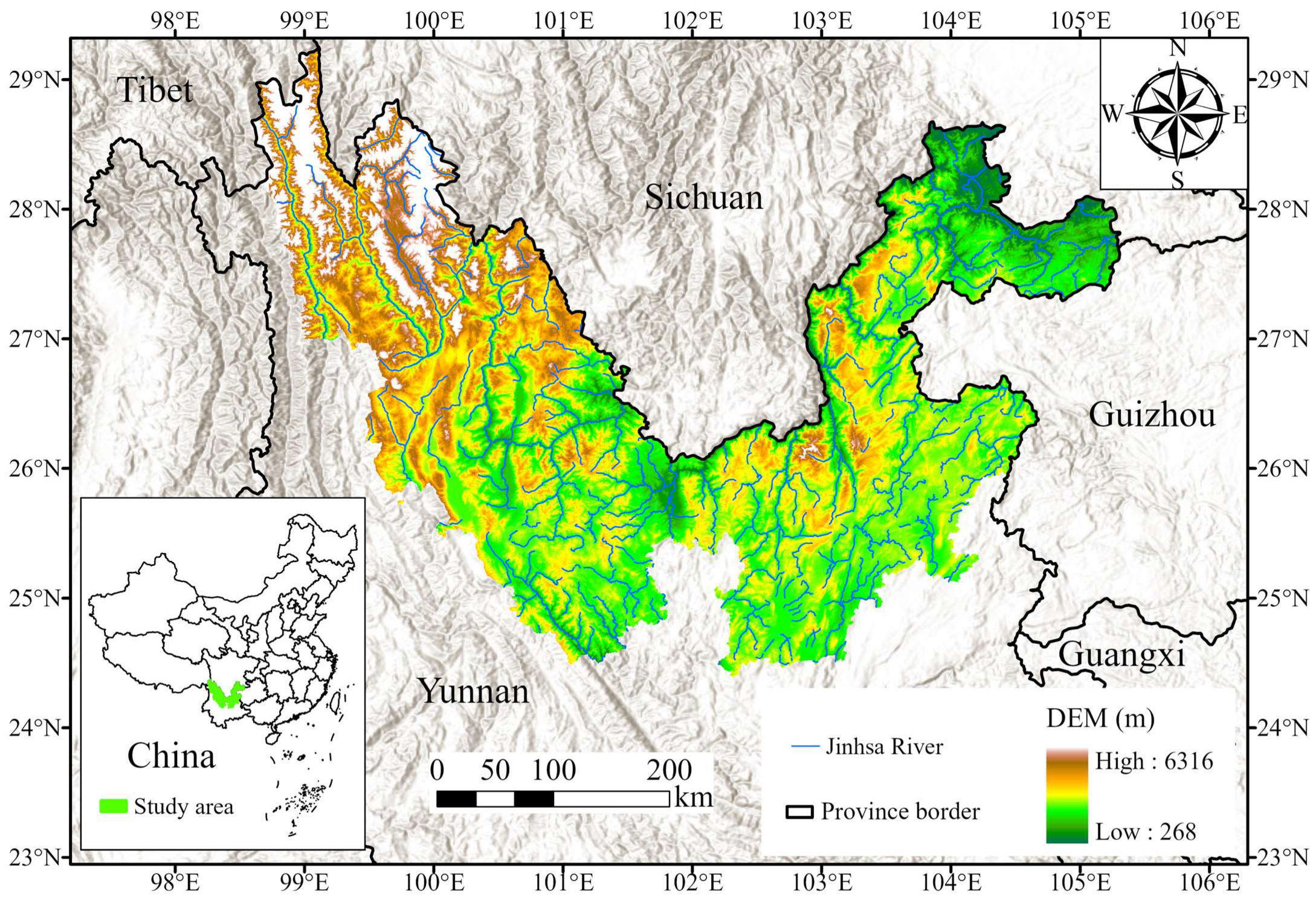
2.1. Research Area

The Jinsha River is a key section of the upper Yangtze River. This study area is located in the northwest, north, and northeast of Yunnan Province, bordering Tibet, Sichuan, and Guizhou (Figure 1). The basin stretches from 98°60′ E to 105°40′ E and from 24°30′ N to 29°30′ N, covering an area of 140,929.6 km². The topography is divided into two major regions: the northwest and northeast. The northwest, primarily within the Tibetan Plateau, features alternating high mountains and deep valleys, while the northeast, part of the Yunnan Plateau, consists of intermontane basins. The basin has a plateau temperate humid climate, with an average annual temperature of 15.7 °C and annual precipitation of 828.7 mm. The wet season, from May to October, accounts for over 80% of the yearly rainfall.

2.2. Data Collection and Processing

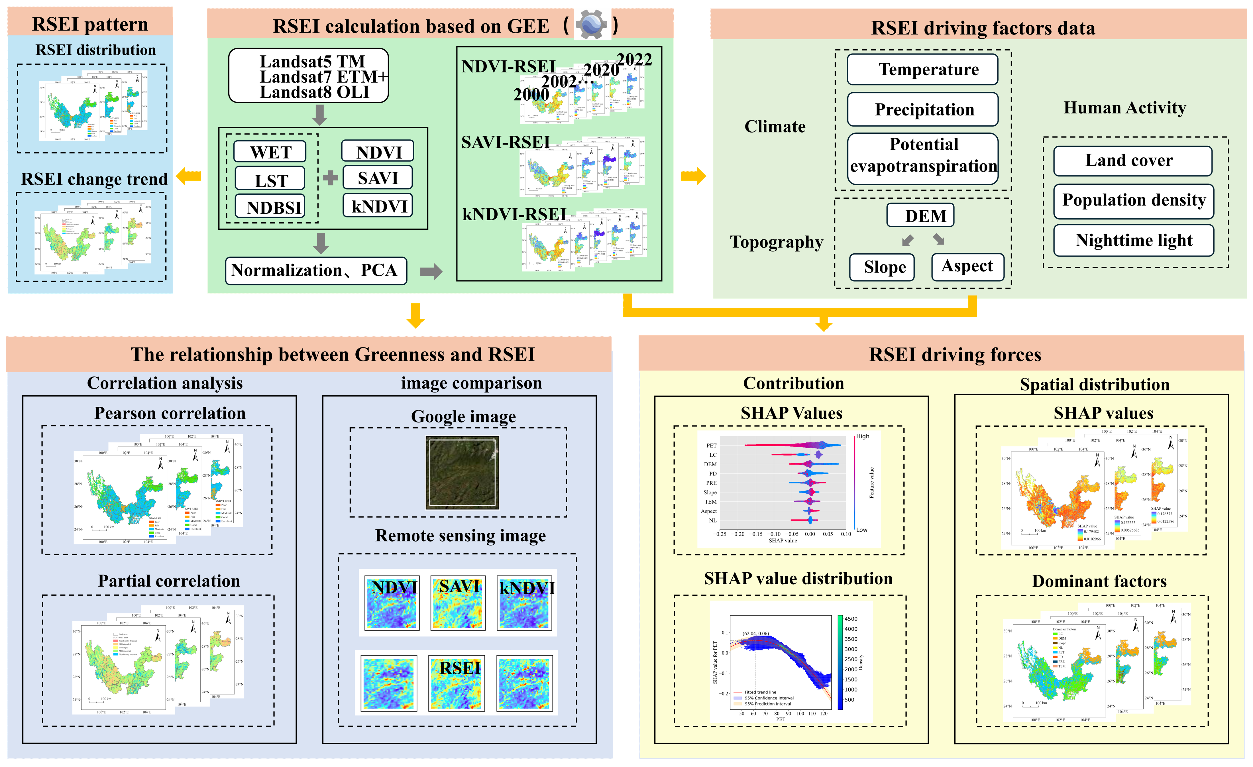
This study used the GEE platform to construct NDVI-RSEI, SAVI-RSEI, and kNDVI-RSEI datasets, covering 12 even-numbered years from 2000 to 2022. RSEI data for 2000–2010 were derived from Landsat 5 (TM), 2012 data from Landsat 7 (ETM+), and 2014–2022 data from Landsat 8 (OLI). To ensure accuracy, water bodies and clouds were masked, and only images from the vegetation growing season (May to October) were used. All Landsat data were corrected for atmospheric aerosols, radiance, and geometric distortions.

Furthermore, the study analyzed nine factors influencing RSEI. By calculating the Variance Inflation Factor (VIF) for each dataset, all VIF values were <10, indicating low multicollinearity among the variables (

Table 1. The data source of driving factors.

Category	Metrics	Abbreviation	Spatial Resolution	Time Resolution	Year	Source	VIF
Climate	precipitation	PRE	1 km	1 month	2000–2022	https://data.tpdc.ac.cn/ (accessed on 3 September 2024) [32]	2.38
	temperature	TEM	1 km	1 month	2000–2022	https://data.tpdc.ac.cn/ (accessed on 3 September 2024) [33]	5.41
	potential evapotranspiration	PET	1 km	1 month	2000–2022	https://data.tpdc.ac.cn/ (accessed on 3 September 2024) [34]	2.44
Topography	DEM	DEM	30 m	-	-	https://portal.opentopography.org/ (accessed on 3 September 2024)	6.42
	slope	Slope	30 m	-	-		1.18
	aspect	Aspect	30 m	-	-		1.01
Human Activity	land cover	LC	30 m	1 year	2000–2022	https://zenodo.org/records/12779975 (accessed on 3 September 2024)	1.07
	population density	PD	1 km	1 year	2000–2022	https://landscan.ornl.gov/ (accessed on 3 September 2024)	1.19
	nighttime light	NL	1 km	1 year	2000–2022	https://dataverse.harvard.edu/ (accessed on 3 September 2024) [35]	1.27

). These nine factors were grouped into three categories: climate, topography, and human activities. Climate data, including precipitation [32], temperature [33], and potential evapotranspiration [34], were provided by the National Tibetan Plateau Data Center. Topographic data were based on the Copernicus Digital Elevation Model (DEM) from the European Space Agency (ESA), with slope and aspect derived from the DEM. Human activity data, including land cover, was classified into nine types: Cropland, Forest, Shrub, Grassland, Water, Snow/Ice, Barren, Impervious, and Wetland. Population density data came from the LandScan dataset, representing population per raster cell. Nighttime Light data were derived from a calibrated DMSP-OLS dataset using the “pseudo-invariant feature” method, which addressed temporal discrepancies between DMSP-OLS and SNPP-VIIRS data and repaired missing data in the original SNPP-VIIRS monthly dataset to create an improved DMSP-OLS-like dataset [35].

2.3. Methods

Figure 2 presents the technical flowchart of this study. First, following the RSEI calculation method [36], the greenness indicator was extended from NDVI to SAVI and kNDVI. Landsat TM/ETM+/OLI imagery was used to obtain the long-term spatiotemporal distribution of three RSEI types (NDVI-RSEI, SAVI-RSEI, and kNDVI-RSEI) for even-numbered years between 2000 and 2022 in the Jinsha River Basin, Yunnan Province. The Theil–Sen median method and Mann–Kendall trend analysis were applied to analyze RSEI trends. Pearson correlation and partial correlation analyses were performed to examine the relationship between greenness and RSEI, highlighting differences in their remote sensing details. Finally, XGBoost and SHAP models were used to assess the importance of RSEI-influencing factors across three dimensions—climate, topography, and human activities—and to map the spatial distribution of dominant factors and SHAP values in the study area.

2.3.1. Construction of RSEI

RSEI is constructed using four indicators: greenness (NDVI), heat (LST), humidity (WET), and dryness (NDBSI), collectively referred to as NDVI-RSEI [37]. NDVI and WET are considered positive ecological factors, while LST and NDBSI are negative factors. To investigate differences in RSEI calculated using various greenness indicators and to analyze the impact of greenness on RSEI outcomes, this study replaced the greenness indicator with SAVI and kNDVI, while keeping heat, humidity, and dryness unchanged, resulting in SAVI-RSEI and kNDVI-RSEI. The specific calculation methods are detailed in

Table 2. Calculation methods for ecological indicators.

Ecological Factors	RSEI Indices	Equations	Explanation
Greenness	NDVI	$NDVI={\displaystyle \frac{{\rho }_{NIR}-{\rho }_{Red}}{{\rho }_{NIR}+{\rho }_{Red}}}$	${\rho }_{NIR}$ represents the reflectance in the near-infrared band; ${\rho }_{Red}$ represents the reflectance in the red band [36].
	SAVI	$SAVI={\displaystyle \frac{({\rho }_{NIR}-{\rho }_{Red})\times (1+L)}{({\rho }_{NIR}+{\rho }_{Red}+L)}}$	$L$ is the soil adjustment factor, typically set to 0.5 [38].
	kNDVI	$kNDVI=tanh\left({\left({\displaystyle \frac{{\rho }_{NIR}-{\rho }_{Red}}{2\sigma }}\right)}^2\right)$	$\sigma$ represents the length scale parameter, indicating the sensitivity of the index to areas with sparse or dense vegetation. It is commonly assigned an average value of $\sigma =0.5({\rho }_{NIR}+{\rho }_{Red})$, allowing the formula to be simplified as $kNDVI=\mathrm{t}\mathrm{a}\mathrm{n}\mathrm{h}\left({NDVI}^2\right)$ [23].
Humidity	WET	$\begin{array}{c}WE{T}_{TM}=0.0315{\rho }_{Blue}+0.2021{\rho }_{Green}+0.3102{\rho }_{Red}+\\ 0.1594{\rho }_{NIR}-0.6806{\rho }_{SWIR1}-0.6109{\rho }_{SWIR2}\end{array}$	${\rho }_{Blue}$, ${\rho }_{Green}$, ${\rho }_{Red}$, ${\rho }_{SWIR1}$, and ${\rho }_{SWIR2}$ represent the bands of remote sensing imagery [36].
		$\begin{array}{c}WE{T}_{ETM+}=0.0315{\rho }_{Blue}+0.2021{\rho }_{Green}+0.3102{\rho }_{Red}+\\ 0.1594{\rho }_{NIR}-0.6806{\rho }_{SWIR1}-0.6109{\rho }_{SWIR2}\end{array}$
		$\begin{array}{c}WE{T}_{OLI}=0.1511{\rho }_{Blue}+0.1973{\rho }_{Green}+0.3283{\rho }_{Red}+\\ 0.3407{\rho }_{NIR}-0.7117{\rho }_{SWIR1}-0.4559{\rho }_{SWIR2}\end{array}$
Heat	LST	$LST=T/[1+(\lambda T/\rho )\times \mathrm{i}\mathrm{n}\epsilon ]-273.15$	This calculation approach follows the methodology outlined in [39].
Dryness	NDBSI	$\begin{array}{c}NDBSI=(SI+IBI)/2\\ SI={\displaystyle \frac{({\rho }_{SWIR1}+{\rho }_{Red})-({\rho }_{NIR}+{\rho }_{Blue})}{({\rho }_{SWIR1}+{\rho }_{Red})+({\rho }_{NIR}+{\rho }_{Blue})}}\\ IBI={\displaystyle \frac{\frac{2{\rho }_{SWIR1}}{{\rho }_{SWIR1}+{\rho }_{NIR}}-\left[\frac{{\rho }_{NIR}}{{\rho }_{NIR}+{\rho }_{Red}}+\frac{{\rho }_{Green}}{{\rho }_{Green}+{\rho }_{SWIR1}}\right]}{\frac{2{\rho }_{SWIR1}}{{\rho }_{SWIR1}+{\rho }_{NIR}}+\left[\frac{{\rho }_{NIR}}{{\rho }_{NIR}+{\rho }_{Red}}+\frac{{\rho }_{Green}}{{\rho }_{Green}+{\rho }_{SWIR1}}\right]}}\end{array}$	${\rho }_{Blue}$, ${\rho }_{Green}$, ${\rho }_{Red}$, ${\rho }_{SWIR1}$, and ${\rho }_{SWIR2}$ represent the bands of remote sensing imagery. $SI$ is the soil index; $IBI$ is the index-based built-up index [36].

.

$$\begin{array}{c}{RSEI}_{NDVI}=f\left(NDVI,LST,WET,NDBSI\right)\\ {RSEI}_{SAVI}=f\left(SAVI,LST,WET,NDBSI\right)\\ {RSEI}_{kNDVI}=f\left(kNDVI,LST,WET,NDBSI\right)\end{array}$$

(1)

Principal component analysis (PCA) is applied to integrate the four indicators, with the first principal component being defined as ${RSEI}_0$, as follows:

$$\begin{array}{c}{RSEI}_{{NDVI}_0}=1-PC1\left[f\left(NDVI,LST,WET,NDBSI\right)\right]\\ {RSEI}_{{SAVI}_0}=1-PC1\left[f\left(SAVI,LST,WET,NDBSI\right)\right]\\ {RSEI}_{{kNDVI}_0}=1-PC1\left[f\left(kNDVI,LST,WET,NDBSI\right)\right]\end{array}$$

(2)

Finally, the RSEI is normalized using the following equation:

$$RSEI={\displaystyle \frac{{RSEI}_0-{RSEI}_{0min}}{{RSEI}_{0max}-{RSEI}_{0min}}}$$

(3)

where ${RSEI}_0$ is the first principal component of the four indicators, $RSEI$ is the remote sensing ecological index, ${RSEI}_{0min}$ is the minimum value of ${RSEI}_0$, and ${RSEI}_{0max}$ is the maximum value of ${RSEI}_0$. The $RSEI$ value ranges between 0 and 1, with values closer to 1 indicating better ecological environment quality, and values closer to 0 indicating worse ecological environment quality.

This paper utilizes PCA with three greenness indicators—NDVI, SAVI, and kNDVI—each combined with WET, LST, and NDBSI, to construct three RSEI models: NDVI-RSEI, SAVI-RSEI, and kNDVI-RSEI. As shown in

Table 3. Loading values of the greenness index, the eigenvalue, and the contribution of PC1.

Year	Loading Value			Eigenvalue			Contribution Rate/%
	NDVI	SAVI	kNDVI	NDVI-RSEI	SAVI-RSEI	kNDVI-RSEI	NDVI-RSEI	SAVI-RSEI	kNDVI-RSEI
2000	0.55	0.42	0.69	0.03	0.03	0.04	66.94	61.26	69.80
2002	0.62	0.55	0.85	0.01	0.01	0.02	65.75	61.62	75.49
2004	0.65	0.50	0.76	0.03	0.02	0.04	83.42	79.20	85.71
2006	0.72	0.46	0.79	0.03	0.02	0.03	81.53	74.64	84.53
2008	0.62	0.34	0.71	0.02	0.02	0.03	74.50	71.26	75.96
2010	0.67	0.56	0.76	0.03	0.02	0.04	81.07	75.41	82.74
2012	0.56	0.35	0.70	0.04	0.03	0.05	72.25	68.00	74.48
2014	0.42	0.87	0.84	0.02	0.02	0.03	66.51	53.63	69.85
2016	0.48	0.89	0.86	0.01	0.02	0.03	63.88	59.19	70.58
2018	0.34	0.93	0.86	0.01	0.02	0.03	62.29	55.35	65.44
2020	0.36	0.68	0.81	0.02	0.02	0.03	67.97	56.27	68.81
2022	0.79	0.90	0.88	0.02	0.02	0.02	66.70	66.53	74.28

, the loading values of NDVI, SAVI, and kNDVI are all positive, reflecting the positive influence of greenness on ecological quality, consistent with real-world observations. The magnitude of the eigenvalues represents the amount of information contained in the eigenvectors, and a comparison of these values indicates that all three RSEI models effectively capture the information from the greenness indicators. The contribution rate of PC1 consistently exceeds 60%, demonstrating that PC1 encapsulates most of the characteristic information from the original indicators.

2.3.2. Trend Analysis

The Theil–Sen median method is a robust non-parametric statistical approach for trend estimation [40]. It is computationally efficient and resistant to outliers [41]. Therefore, this method was used in this study to calculate the trend direction of RSEI in the Jinsha River Basin from 2000 to 2022. The calculation equation is as follows:

$${\beta }_{RSEI}=Median\left({\displaystyle \frac{{RSEI}_j-{RSEI}_i}{j-i}}\right),\forall i<j,1\le i<j\le N$$

(4)

where ${RSEI}_i$ and ${RSEI}_j$ represent the $RSEI$ values in year $i$ and $j$, respectively; $Median$ is the median function; $N$ is the sample size; and ${\beta }_{RSEI}$ is the median slope between any two points.

The Mann–Kendall test is a non-parametric test commonly used as a complement to the Sen slope estimator to determine the significance of trends in time series data. In this study, the Mann–Kendall trend test was used to reveal the autocorrelation in the RSEI time series, and the significant trends were identified at the p < 0.05 level. The calculation formulas are as follows:

$$S=\sum _{i=1}^{n-1} \sum _{j=i+1}^n sign(RSE{I}_j-RSE{I}_i)$$

(5)

$$\mathrm{s}\mathrm{i}\mathrm{g}\mathrm{n}(RSE{I}_j-RSE{I}_i)=\left\{\begin{array}{c}+1,RSE{I}_j-RSE{I}_i>0\\ 0,RSE{I}_j-RSE{I}_i=0\\ -1,RSE{I}_j-RSE{I}_i<0\end{array}\right.$$

(6)

$$Var(S)={\displaystyle \frac{n(n-1)(2n+5)}{18}}$$

(7)

$$Z=\left\{\begin{array}{c}(S-1)/\sqrt{Var\left(S\right)},S>0\\ 0,S=0\\ (S-1)/\sqrt{Var\left(S\right)},S<0\end{array}\right.$$

(8)

where $n$ is the number of observations in the time series; $RSE{I}_i$ and $RSE{I}_j$ are the $RSEI$ values for year $i$ and year $j$, respectively; and $Var\left(S\right)$ is the variance. The results of RSEI trend analysis were obtained by combining the Theil–Sen median trend method with the Mann–Kendall test, and the trend types were classified into five categories in

Table 4. RSEI Trend Classification.

${\mathit{\beta }}_{\mathit{R}\mathit{S}\mathit{E}\mathit{I}}$	Z	RSEI Trend
${\beta }_{RSEI}>0.0005$	$\left|\mathrm{Z}\right|>1.96$	Significantly improved
${\beta }_{RSEI}>0.0005$	$\left|\mathrm{Z}\right|\le$ 1.96	Mildly improved
−0.0005 $\le {\beta }_{RSEI}\le$ 0.0005	$\left|\mathrm{Z}\right|\le$ 1.96	Unchanged
${\beta }_{RSEI}<-0.0005$	$\left|\mathrm{Z}\right|\le 1.96$	Mildly degraded
${\beta }_{RSEI}<-0.0005$	$\left|\mathrm{Z}\right|>1.96$	Significantly degraded

.

2.3.3. Correlation Analysis

The Pearson correlation coefficient is a linear correlation coefficient that indicates the degree of linear relationship between two variables, $X$ and $Y$, and is represented by $r$ [42]. We used the Pearson correlation coefficient to preliminarily analyze the relationship between greenness indicators (NDVI, SAVI, kNDVI) and their corresponding RSEI (NDVI-RSEI, SAVI-RSEI, kNDVI-RSEI).

$$r={\displaystyle \frac{\sum _{i=1}^n (X_i-\overline{X})(Y_i-\overline{Y})}{\sqrt{\sum _{i=1}^n (X_i-\overline{X}{)}^2}\sqrt{\sum _{i=1}^n {\left(Y_i-\overline{Y}\right)}^2}}}$$

(9)

where $X_i$ represents the greenness value in the year, $\overline{X}$ is the mean greenness value for even-numbered years from 2000 to 2022, $Y_i$ represents the RSEI value in year $i$, and $\overline{Y}$ is the mean RSEI value for even-numbered years from 2000 to 2022. The $r$ value ranges from −1 to 1, with larger values indicating a stronger correlation. When $r$ > 0, it indicates a positive relationship between the two variables; when $r$ < 0, it indicates a negative relationship. When $r$ = 0, no linear relationship exists between the two variables.

Specifically, we calculated r(NDVI, NDVI-RSEI), representing the correlation between NDVI and NDVI-RSEI. Similarly, we calculated r(SAVI, SAVI-RSEI) and r(kNDVI, kNDVI-RSEI), which represent the correlation between SAVI and SAVI-RSEI and between kNDVI and kNDVI-RSEI, respectively. Given the interactions between ecological factors, it is essential to control for the influence of the factors (WET, LST, NDBSI) used in constructing RSEI when analyzing the correlation between greenness and RSEI. Therefore, we used partial correlation analysis, denoted as $P{r}_{XY\cdot Z_1{Z}_2{Z}_3}$ [43,44].

$$P{r}_{XY\cdot Z_1{Z}_2{Z}_3}={\displaystyle \frac{r_{XY}-r_{X{Z}_1}{r}_{Y{Z}_1}-r_{X{Z}_2}{r}_{Y{Z}_2}-r_{X{Z}_3}{r}_{Y{Z}_3}}{\sqrt{(1-r_{X{Z}_1}^2-r_{X{Z}_2}^2-r_{X{Z}_3}^2)(1-r_{Y{Z}_1}^2-r_{Y{Z}_2}^2-r_{Y{Z}_3}^2)}}}$$

(10)

where $X$ represents greenness; $Y$ represents RSEI; $r_{XY}$ is the Pearson correlation coefficient between greenness and RSEI; $Z_1$ represents WET; $Z_2$ represents LST; $Z_3$ represents NDBSI; and $r_{X{Z}_1}$, $r_{X{Z}_2}$, and $r_{X{Z}_3}$ are the Pearson correlation coefficients between greenness and the control variables (WET, LST, and NDBSI), respectively. Similarly, $r_{Y{Z}_1}$, $r_{Y{Z}_2}$, and $r_{Y{Z}_3}$ are the Pearson correlation coefficients between RSEI and the control variables (WET, LST, and NDBSI), respectively.

Specifically, we calculated Pr(NDVI, NDVI-RSEI), representing the partial correlation between NDVI and NDVI-RSEI while controlling for the effects of other ecological factors. Similarly, we calculated Pr(SAVI, SAVI-RSEI) and Pr(kNDVI, kNDVI-RSEI), representing the partial correlation between SAVI and SAVI-RSEI and between kNDVI and kNDVI-RSEI, respectively. Through partial correlation analysis, we can qualitatively determine the influence of different greenness indicators on RSEI and their changing trends.

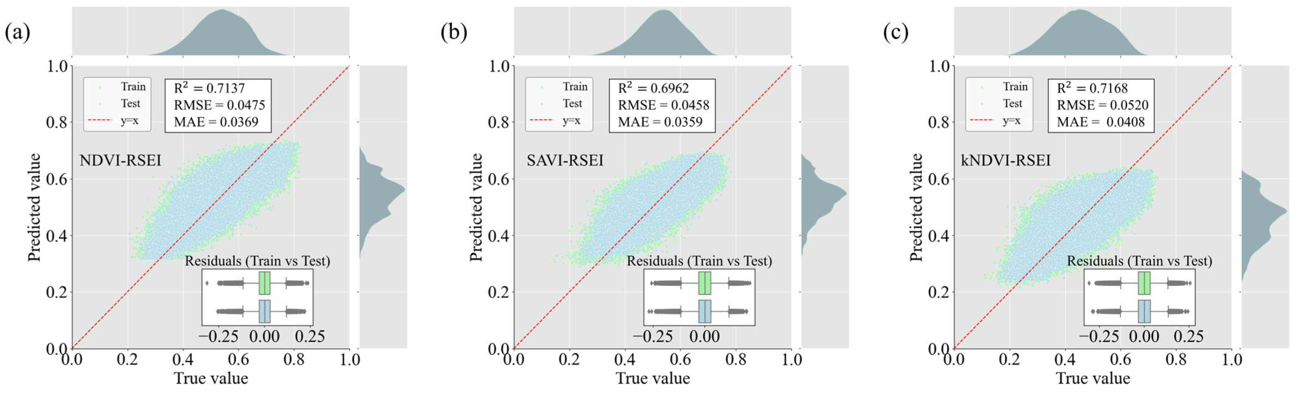
2.3.4. Explainable Machine Learning

XGBoost, an enhanced version of the gradient-boosted decision tree algorithm, is known for its excellent performance in handling sparse datasets [28]. In this study, we used XGBoost to investigate the factors driving changes in RSEI, including precipitation, temperature, potential evapotranspiration, DEM, slope, aspect, land use type, population density, and nighttime lights (Table 2). The dataset was randomly split into 70% for training and 30% for testing to evaluate the model’s performance. Model accuracy was assessed through regression analysis of the predicted and observed values in the test dataset, using R², root mean square error (RMSE), and mean absolute error (MAE) as evaluation metrics.

SHAP, based on Shapley values from game theory, explains the output of machine learning models by visualizing complex causal relationships between the dependent variable and its driving factors [29]. The development of SHAP has unlocked significant potential for understanding machine learning models applied to spatial data, as each observation is geographically referenced, enabling the spatial visualization of feature attributions [45]. In this study, SHAP was employed to elucidate the nonlinear relationships hidden within the XGBoost model and to translate them into interpretable rules, thereby visualizing the model’s results.

We utilized the XGBoost-SHAP IML model to explore the driving factors of RSEI. During model training, we carefully tuned the XGBoost hyperparameters, selecting the squared log error loss function, 2000 trees, and a learning rate of 0.05. The model training and performance evaluation followed four key steps: (1) the dataset, consisting of 487,346 sets of influencing factors and RSEI data, was randomly split into training and testing sets with a 7:3 ratio; (2) the XGBoost model was constructed, and initial parameters were set; (3) XGBoost hyperparameters were optimized through grid search and five-fold cross-validation, and regularization techniques were applied to prevent overfitting; and (4) the average performance metrics were calculated across five evaluation iterations.

As shown in Figure 3, the performance of the XGBoost model for NDVI-RSEI, SAVI-RSEI, and kNDVI-RSEI was as follows: R² values were 0.7137, 0.6962, and 0.7168, respectively; RMSE values were 0.0475, 0.0458, and 0.0520, respectively; and MAE values were 0.0369, 0.0359, and 0.0408, respectively. These results demonstrate the effectiveness of XGBoost in identifying the driving factors of RSEI.

3. Results

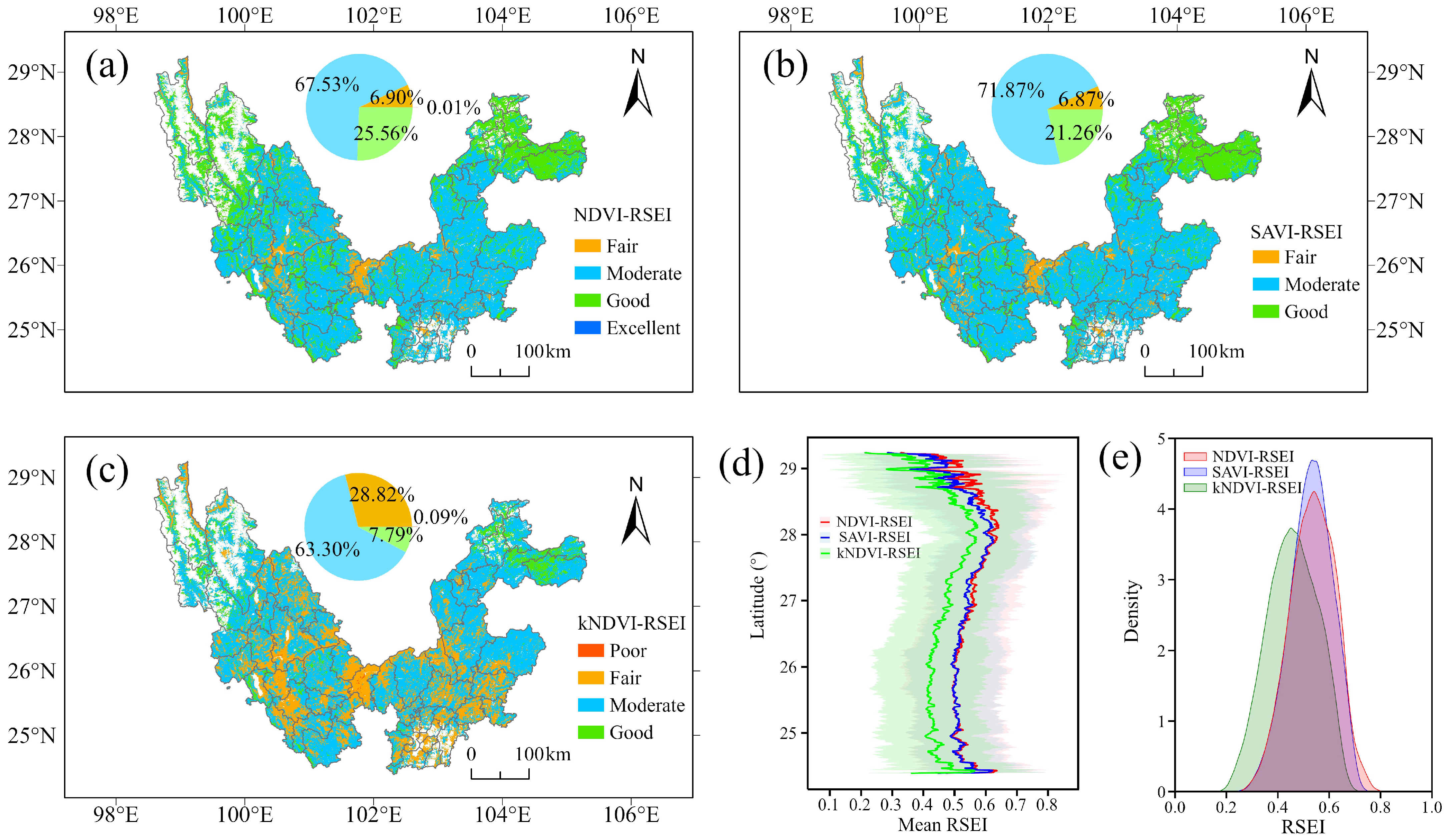
3.1. The Spatiotemporal Pattern of RSEI

3.1.1. The Distribution of RSEI

By calculating NDVI-RSEI, SAVI-RSEI, and kNDVI-RSEI for every even-numbered year from 2000 to 2022, the average spatial distribution of the three RSEI types over 12 years was obtained (Figure 4a–c). Based on existing research [46], the natural breaks method was used to classify RSEI into five categories: poor (0 < RSEI ≤ 0.2), fair (0.2 < RSEI ≤ 0.4), moderate (0.4 < RSEI ≤ 0.6), good (0.6 < RSEI ≤ 0.8), and excellent (0.8 < RSEI ≤ 1). On a spatial scale, the average RSEI levels for even-numbered years between 2000 and 2022 were predominantly moderate, good, and fair, with moderate RSEI covering the largest area, mainly concentrated in the central part of the study region. The percentage of moderate areas for NDVI-RSEI, SAVI-RSEI, and kNDVI-RSEI was 67.53%, 71.87%, and 63.30%, respectively. Additionally, compared to NDVI-RSEI and SAVI-RSEI, the good category in kNDVI-RSEI accounted for only 7.79%, while the fair category reached 28.82%.

According to the latitudinal distribution of average RSEI values (Figure 4d), the distribution patterns of NDVI-RSEI, SAVI-RSEI, and kNDVI-RSEI were similar, but kNDVI-RSEI exhibited a clear tendency to underestimate RSEI values. Based on the RSEI density distribution (Figure 4e), the NDVI-RSEI density curve followed a roughly normal distribution, while SAVI-RSEI exhibited the most concentrated distribution with the highest peak. In contrast, the kNDVI-RSEI density curve had the widest distribution within the lower ecological quality range.

Figure 5 illustrates the annual average variations of greenness (NDVI, SAVI, and kNDVI) and their corresponding RSEI values (NDVI-RSEI, SAVI-RSEI, and kNDVI-RSEI) from 2000 to 2020. On a temporal scale, vegetation cover and ecological conditions in the Jinsha River Basin remained relatively stable throughout the study period. The 12-year average greenness values ranked as SAVI (0.57) > NDVI (0.51) > kNDVI (0.39), while the average RSEI values followed the order SAVI-RSEI (0.53) > NDVI-RSEI (0.50) > kNDVI-RSEI (0.46).

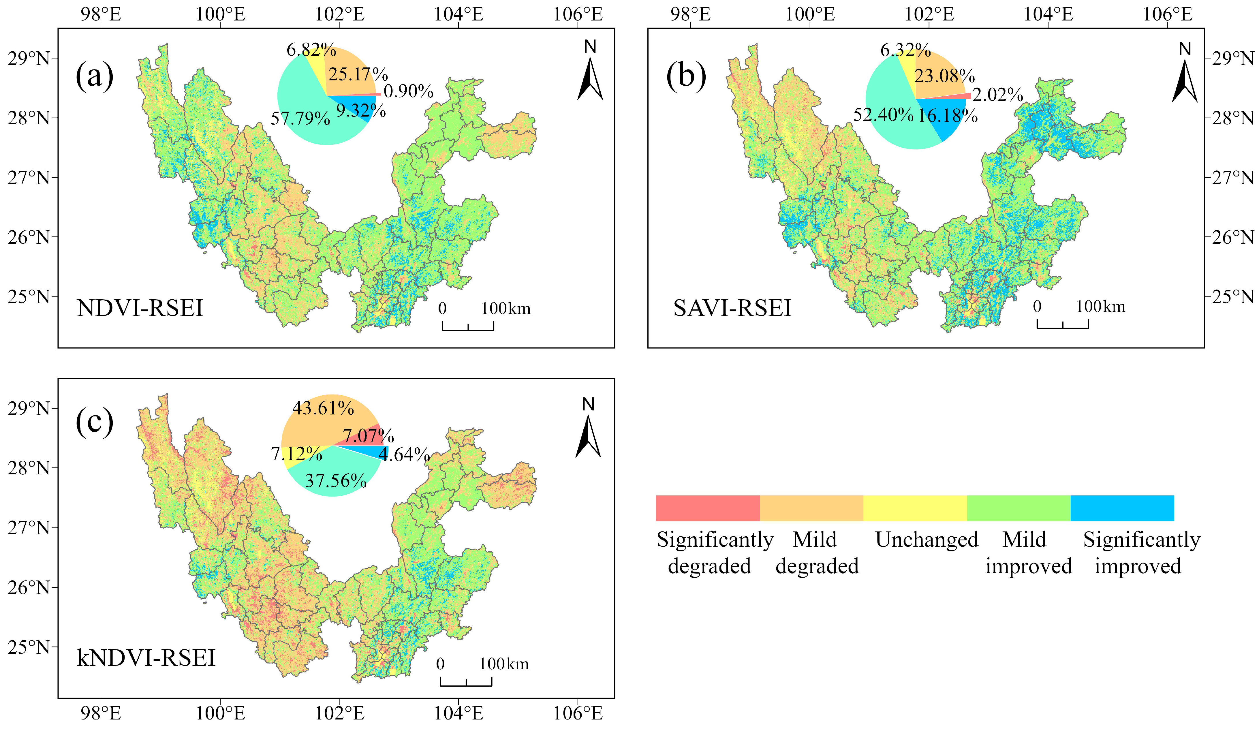
3.1.2. The Trend of RSEI

Based on the changes in the three types of RSEI from 2000 to 2022 in even-numbered years, trend variations were calculated and classified at the pixel level using the method outlined in Table 1. As shown in Figure 6, the RSEI trends were divided into five categories: significantly improved, mildly improved, unchanged, mildly degraded, and significantly degraded. The pie charts represent the percentage of area covered by each trend category. Figure 6a,b shows that the overall trends of NDVI-RSEI and SAVI-RSEI were positive, covering 67.11% and 68.58% of the study area, respectively. From a spatial distribution perspective, environmental improvement is observed in the eastern region of the study area, while the western region shows environmental degradation. However, compared to the other two types of RSEI, kNDVI-RSEI (Figure 6c) reveals that the area of environmental improvement only accounts for 42.20% of the total area.

3.2. The Relationship Between Greenness and RSEI

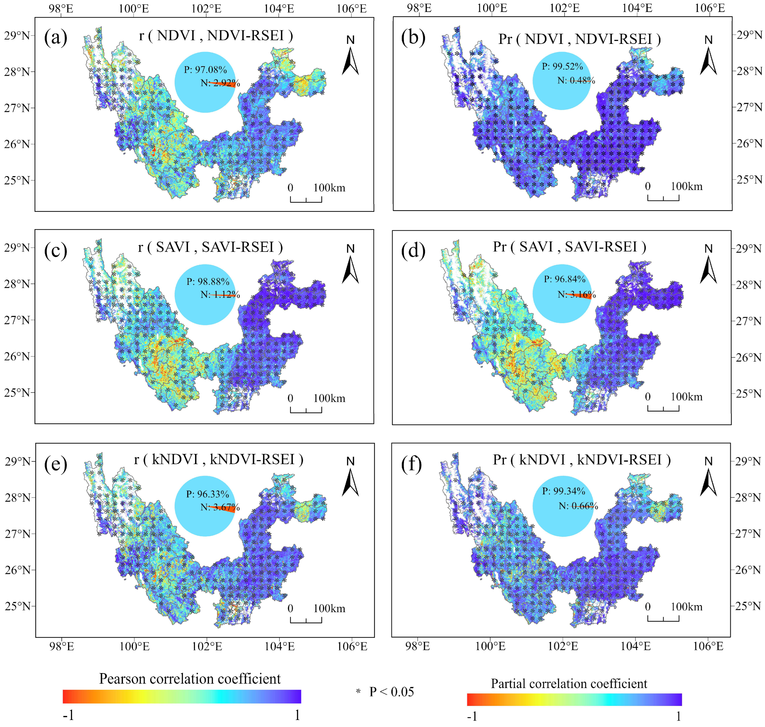
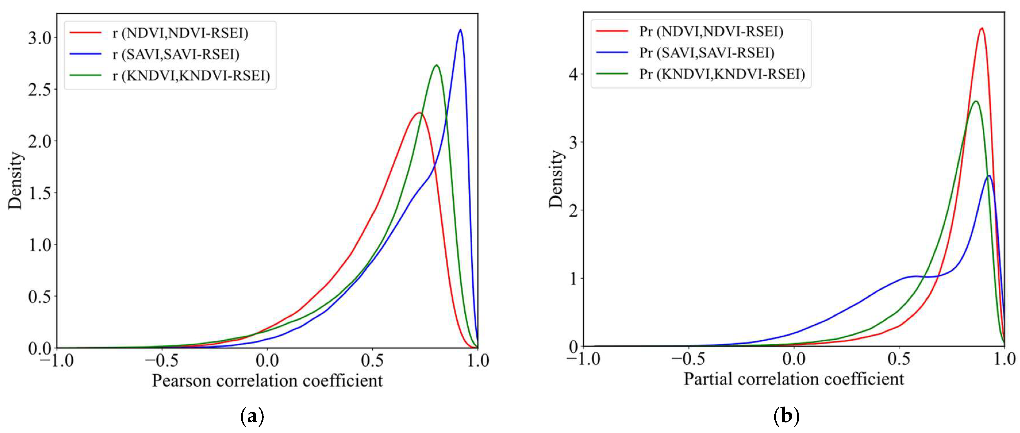
3.2.1. Correlation Analysis Between Greenness and RSEI

The Pearson correlation analysis between greenness indicators and RSEI (Figure 7a,c,e) reveals a significant positive correlation, with 97.08% (NDVI, NDVI-RSEI), 98.88% (SAVI, SAVI-RSEI), and 96.33% (kNDVI, kNDVI-RSEI) of the areas showing a positive relationship. Regions with strong positive correlations are primarily located in the eastern part of the study area. Figure 8a presents the density distribution of Pearson correlation coefficients between the three greenness indices and their corresponding RSEI values. The strength of Pearson correlation follows the order: r (SAVI, SAVI-RSEI) > r (kNDVI, kNDVI-RSEI) > r (NDVI, NDVI-RSEI). These results suggest that greenness generally promotes RSEI across most areas of the study region. However, whether RSEI changes are primarily driven by greenness or influenced by other factors remains unclear, warranting further investigation into the isolated impact of greenness on RSEI.

Partial correlation analysis was conducted to explore the relationship between greenness and RSEI while controlling for other variables (WET, LST, NDBSI) to eliminate confounding effects. As shown in Figure 7b,d,f, compared to Pearson correlations, the proportion of positive partial correlations between greenness and RSEI increased to 99.52% (NDVI, NDVI-RSEI) and 99.34% (kNDVI, kNDVI-RSEI). However, the proportion of positive partial correlations between SAVI and SAVI-RSEI decreased to 96.84%. Figure 8b illustrates the density distribution of partial correlation coefficients between the greenness indices and their respective RSEI models. The ranking of partial correlations is as follows: PR(NDVI, NDVI-RSEI) > Pr(kNDVI, kNDVI-RSEI) > Pr(SAVI, SAVI-RSEI). These findings indicate that interactions with other variables weakened the correlation between NDVI and NDVI-RSEI, as well as between kNDVI and kNDVI-RSEI, but strengthened the correlation between SAVI and SAVI-RSEI.

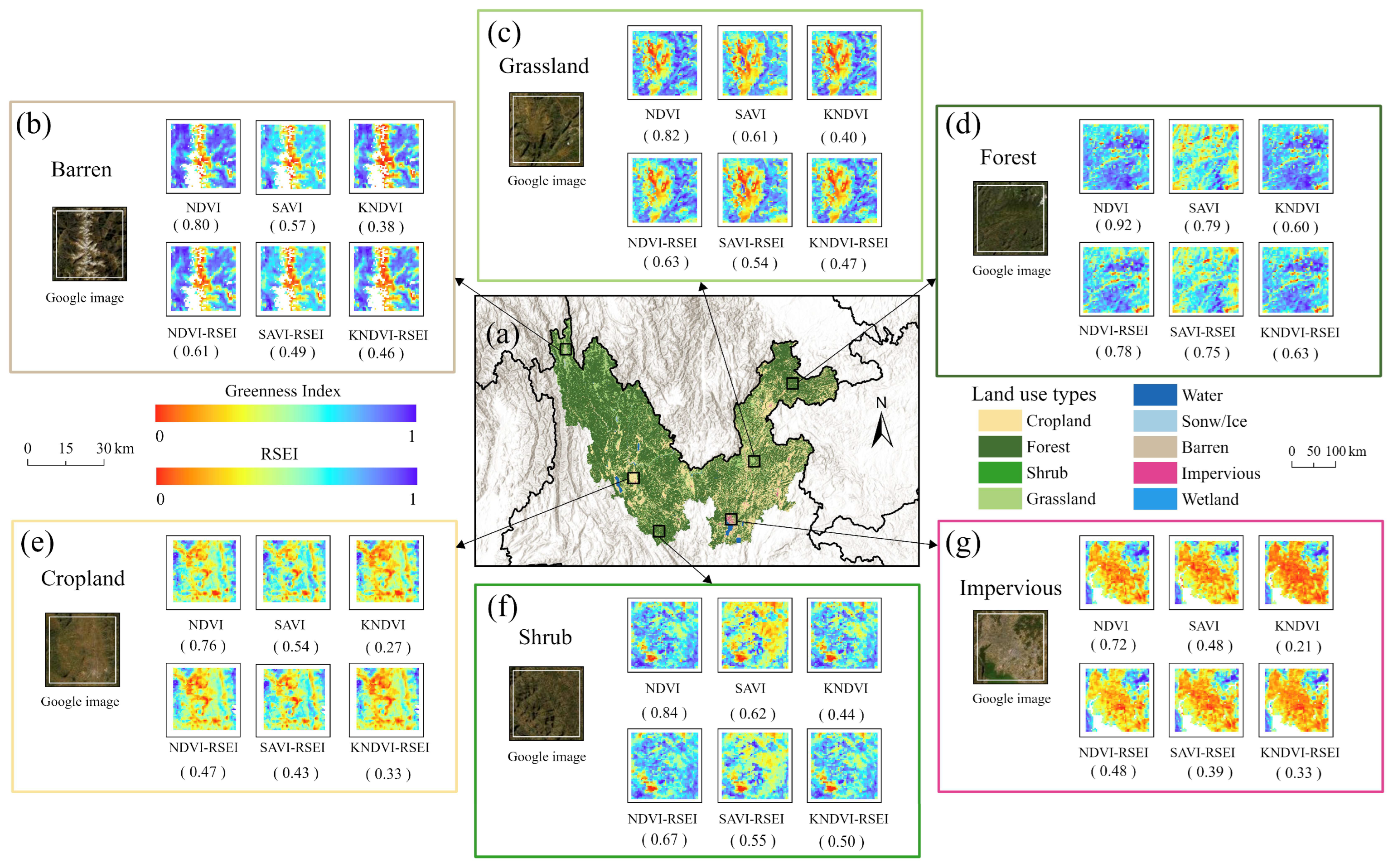
3.2.2. Comparison of Image Details Under Different Land Use Types

Figure 9 illustrates the spatial distribution and evaluation performance of three greenness indices (NDVI, SAVI, and kNDVI) and their corresponding RSEI models (NDVI-RSEI, SAVI-RSEI, kNDVI-RSEI) across different land cover types, including barren (b), grassland (c), forest (d), cropland (e), shrubland (f), and impervious (g). The results reveal notable differences in the performance of the greenness indices and their respective RSEI values across various land cover types. NDVI and NDVI-RSEI exhibit consistent performance in areas with high-density vegetation (forest), accurately reflecting ecological quality in regions with dense vegetation cover. SAVI and SAVI-RSEI show balanced performance in areas with moderate vegetation cover (cropland, shrubland), particularly in regions with strong soil reflectance, demonstrating their ability to reduce soil background interference. Meanwhile, kNDVI and kNDVI-RSEI tend to underestimate ecological quality, but they effectively capture the conditions of low-vegetation cover areas, such as ‘barren’, ‘grassland’, and ‘impervious’.

3.3. Driving Forces of RSEI

3.3.1. Contribution of Driving Forces

We employed a combination of the XGBoost and SHAP models to examine the driving factors influencing RSEI, considering nine variables related to climate, human activities, and topography. The differences among NDVI-RSEI, SAVI-RSEI, and kNDVI-RSEI were primarily attributed to climate factors, accounting for 42.0%, 45.2%, and 40.7%, respectively. PET emerged as the most significant variable, with average SHAP values of 0.0335, 0.0309, and 0.0358, respectively (Figure 10). The analysis reveals that as PET increases, SHAP values also rise. However, once PET exceeds certain thresholds (62.04, 66.36, 64.24, respectively), its positive contribution begins to weaken and may even turn negative (Figure 11a,d,g). This could be due to high PET values corresponding to extreme drought conditions, which negatively impact the ecological environment [47].

In addition to climate factors, human activity variables (accounting for 38.3%, 31.4%, and 37.7% of NDVI-RSEI, SAVI-RSEI, and kNDVI-RSEI, respectively) also play a significant role in explaining RSEI variations. Among these, LC is the most influential, with average SHAP values of 0.0281, 0.0214, and 0.0304, respectively (Figure 10b,d,f). The results (Figure 11b,e,h) indicate that high vegetation cover, such as forests, is associated with higher SHAP values and positive contributions to RSEI. In contrast, land types heavily impacted by human activities (cropland, shrubland, grassland, impervious, barren) display more dispersed SHAP values and exert negative effects on RSEI.

Although the distribution of SHAP values is similar across the three RSEI models for different land types, the focus varies. NDVI-RSEI (Figure 11b) shows relatively high sensitivity to vegetation, resulting in a stronger positive contribution (SHAP value of 0.0234), while land types with lower vegetation cover exhibit more pronounced negative impacts. SAVI-RSEI (Figure 11e) effectively reduces soil reflectance interference, resulting in smaller negative contributions in low-vegetation areas (cropland, shrubland, and grassland), demonstrating its ability to address soil reflectance issues. kNDVI-RSEI (Figure 11h) marginally increased the positive contribution in forest areas (SHAP value of 0.0255) while exhibiting enhanced negative contributions across other land cover types (SHAP values of −0.0253, −0.0165, −0.0710, −0.0847, and −0.0690 for cropland, shrubland, grassland, barren, and impervious surfaces, respectively). This pattern explains the relatively low kNDVI values observed in the analysis.

Topographical factors (accounting for 19.7%, 23.4%, and 21.6% of NDVI-RSEI, SAVI-RSEI, and kNDVI-RSEI, respectively) also significantly contribute to explaining RSEI variation (Figure 10a,c,e). Among these, DEM is the most significant, with average SHAP values of 0.0117, 0.0155, and 0.0156, respectively (Figure 10b,d,f). The results (Figure 11c,f,i) show that as DEM increases, SHAP values gradually decrease, turning the contribution negative. However, once DEM exceeds certain thresholds (3658.18, 4270.37, 3589.18, respectively), the negative contribution of DEM begins to diminish. This may be due to the non-monotonic relationship between elevation and species richness [48].

3.3.2. The Spatial Distribution of Dominant Driving Factors

Figure 12 illustrates the spatial contributions of driving factors for RSEI. In terms of the spatial distribution of dominant factors (Figure 12 a,c,e), the northeastern part of the study area is primarily influenced by DEM, the southeastern region by LC, while other areas are predominantly governed by PET. The percentage of the study area covered by dominant factors varies across the three RSEI models (Figure 13). For NDVI-RSEI (Figure 13a), PET dominates 45.82% of the area, LC covers 42.52%, and DEM accounts for 9.35%. For SAVI-RSEI (Figure 13b), PET covers 48.31%, LC covers 31.48%, and DEM accounts for 14.30%. For kNDVI-RSEI (Figure 12c), PET covers 44.78%, LC covers 41.08%, and DEM accounts for 11.23%.

In terms of the spatial distribution of SHAP values for the dominant factors (Figure 12b,d,f), the three RSEI models exhibit similar patterns, with higher SHAP values in the central and western regions and lower values in the eastern region. Figure 14 shows the density curves corresponding to Figure 12b,d,f. The SHAP value density curves for NDVI-RSEI, SAVI-RSEI, and kNDVI-RSEI follow similar trends, with higher densities at lower SHAP values and lower densities at higher SHAP values. Compared to the other two models, SAVI-RSEI reaches a peak in its density curve at lower SHAP values, indicating that when SHAP values are low—meaning the dominant factors contribute less to RSEI—SAVI-RSEI has the strongest explanatory power. The density curves for NDVI-RSEI and kNDVI-RSEI exhibit similar trends at lower SHAP values, but kNDVI-RSEI shows a higher density at the upper-SHAP-value range. This suggests that while the contribution patterns of dominant factors in NDVI-RSEI and kNDVI-RSEI are similar, kNDVI-RSEI more effectively captures factors with a greater impact on ecological quality.

4. Discussion

4.1. Spatial Distribution and Driving Factors of RSEI

Previous studies have primarily focused on using RSEI to analyze the spatial and temporal distribution of ecological quality, with relatively few investigations exploring the potential expansion of greenness indicators used to construct RSEI. Our results show that RSEIs constructed with different greenness indices effectively capture the spatial variability of ecological environments, and the three RSEIs (NDVI-RSEI, SAVI-RSEI, kNDVI-RSEI) exhibit remarkably similar capabilities in assessing ecological environments (Figure 4). In the Jinsha River Basin of Yunnan Province, these RSEIs demonstrate comparable spatial distribution patterns and driving mechanisms. The RSEI categories can primarily be divided into three types: ‘moderate’ in the southeastern region, ‘good’ in the northeastern region, and ‘fair’ in central areas such as Yuanmou, Yongren, Yongsheng, and Binchuan.

However, the reasons for spatial differences in these RSEI categories vary. The spatial distribution of RSEI driving factors (Figure 12) indicates that in the southeastern region, RSEI is mainly driven by land use types, as this area has a higher proportion of cropland and impervious surfaces, heavily influenced by human activities. In the northeastern region, RSEI is primarily driven by DEM, as this area has elevation differences of up to 1500 m with high vegetation coverage. In central areas like Yuanmou, Yongren, Yongsheng, and Binchuan counties, RSEI is largely influenced by PET due to the region’s location in the hot–dry valley of the Jinsha River. This area is characterized by a hot, arid climate; significant seasonal wet–dry variations; uneven rainfall distribution; and high evaporation, leading to severe vegetation and soil degradation [49].

These phenomena are supported by previous studies. Research has shown that cropland and construction land in the southeastern part of the Jinsha River Basin are concentrated due to rapid urbanization, with a significant increase in construction land [50]. The northeastern region of Yunnan, located in canyon areas along rivers, experiences a maximum terrain relief of up to 1535 m, a notable feature of the Yunnan Plateau’s vertical drop in mountainous terrain [51]. The hot–dry valleys in southwestern China, including Yuanmou County, are severely affected by gully erosion, contributing to ecosystem fragility [52,53].

In conclusion, this study demonstrates that RSEI models constructed with different greenness indices (NDVI, SAVI, kNDVI) effectively assess the spatial heterogeneity of ecological quality while exhibiting high consistency. This consistency results from the synergistic effects of climate, topography, and human activities, reflecting the ecosystem complexity in the study area. Our research not only reveals the spatiotemporal patterns of ecological quality and its key driving factors but also contributes to evidence-based regional sustainable development. Notably, through identifying the primary driving factors and their spatial differentiation characteristics, we have established a fundamental framework for further investigation of ecological factors and their interactions with RSEI. These findings provide significant guidance for optimizing RSEI construction methods across different regional contexts, refining the analytical framework of driving mechanisms and enhancing the applicability and accuracy of the RSEI model.

4.2. The Coupling Relationship Between RSEI and Greenness

The only difference between the three RSEIs (NDVI-RSEI, SAVI-RSEI, and kNDVI-RSEI) lies in the greenness indicator used during the PCA process (NDVI, SAVI, kNDVI), which directly affects the performance of the constructed RSEI. Although NDVI, SAVI, and kNDVI are all significantly positively correlated with their respective RSEIs, Pearson and partial correlation analyses (Figure 7 and Figure 8) reveal that the correlation between RSEI and the greenness indicators (NDVI, SAVI, kNDVI) is influenced by non-greenness factors (WET, LST, NDBSI) incorporated into the RSEI model. These ecological factors interact to reduce the correlation between NDVI and kNDVI with their respective RSEIs, while increasing the correlation between SAVI and SAVI-RSEI. One possible reason for this difference is that SAVI includes a soil adjustment factor (L), which reduces its sensitivity to background soil brightness [22] and increases its sensitivity to ecological structure [54], resulting in a larger dynamic range and reduced sensitivity to atmospheric disturbances [55]. Therefore, SAVI-RSEI only demonstrates its advantages when interacting with other ecological factors. This suggests that SAVI-RSEI is better suited for ecological monitoring in areas with complex background conditions. This conclusion is supported by the correlation analysis between SAVI and SAVI-RSEI (Figure 7c,d), especially in sparsely vegetated areas in the western part of the study area, where the correlation increases significantly due to the influence of other ecological factors. In contrast, for NDVI and kNDVI, the interaction of WET, LST, and NDBSI had a negative impact on RSEI. This may be because NDVI and kNDVI primarily reflect chlorophyll content [56]. Notably, NDVI-RSEI is more influenced by non-greenness factors, while kNDVI-RSEI exhibits greater stability than NDVI-RSEI (Figure 8). A possible explanation is that the nonlinear transformation from NDVI to kNDVI partially mitigates the impact of non-greenness factors, making kNDVI-RSEI more robust in capturing ecosystem health [23].

Different land use types contribute differently to the three RSEIs (Figure 9 and Figure 11b,e,h). In high-greenness areas (forest), NDVI-RSEI and kNDVI-RSEI perform well, as both capture high vegetation coverage effectively. However, the positive contribution of forest to SAVI-RSEI is weaker due to the introduction of the soil adjustment factor in SAVI. In low-greenness areas (grassland, barren, impervious surfaces), the negative contribution of kNDVI-RSEI increases significantly, as kNDVI is highly sensitive to soil background. In medium-greenness areas (cropland, shrubland), the negative contribution to SAVI-RSEI is significantly reduced, with SAVI-RSEI performing stably in areas with sparse vegetation and exposed soil due to its ability to reduce soil background interference on RSEI.

It is worth noting that default soil brightness correction factors (L) for SAVI and nonlinear sensitivity factors (σ) for kNDVI were applied, which may affect the ecological assessment results based on SAVI-RSEI and kNDVI-RSEI. Future research should explore the sensitivity of these greenness indices to their respective correction factors [57,58]. Additionally, when using different greenness indicators as inputs to the RSEI model, adjustments should be made based on the ecological characteristics of the study area to ensure that the RSEI model accurately reflects the state of the ecological environment. These findings offer new insights for future ecological quality assessments, suggesting that combining different ecological indicators to construct a more precise RSEI could improve the accuracy of ecosystem health evaluations.

4.3. Advantages of IML in Identifying Driving Factors

In ecosystems, driving factors often interact in complex, nonlinear ways. Traditional methods for studying the drivers of ecological quality have struggled to capture these nonlinear relationships, and the depth of investigation has often been insufficient. IML models not only identify nonlinear interactions between driving factors but also provide valuable insights into underlying physical processes [59]. In our study, we applied XGBoost to uncover the intricate nonlinear relationships between RSEI and nine driving factors. We used the SHAP method to interpret the trained model, providing quantifiable insights that enhance our conceptual and qualitative understanding of these relationships. The XGBoost-SHAP approach offers several key advantages:

(1)

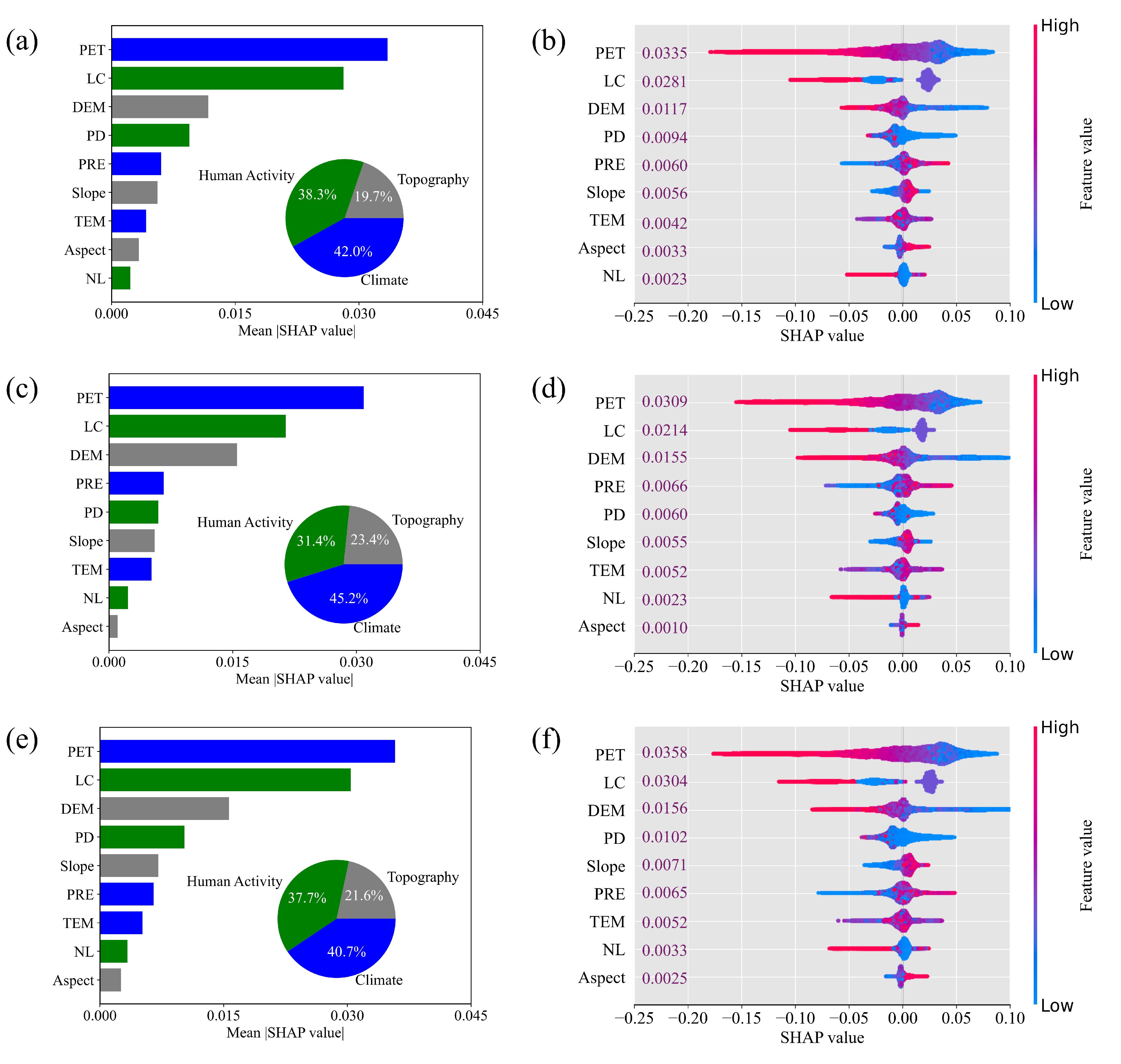
XGBoost-SHAP quantifies the contribution of the nine driving factors to RSEI through feature importance ranking, while intuitively displaying the distribution characteristics of each factor’s contribution (Figure 10).

(2)

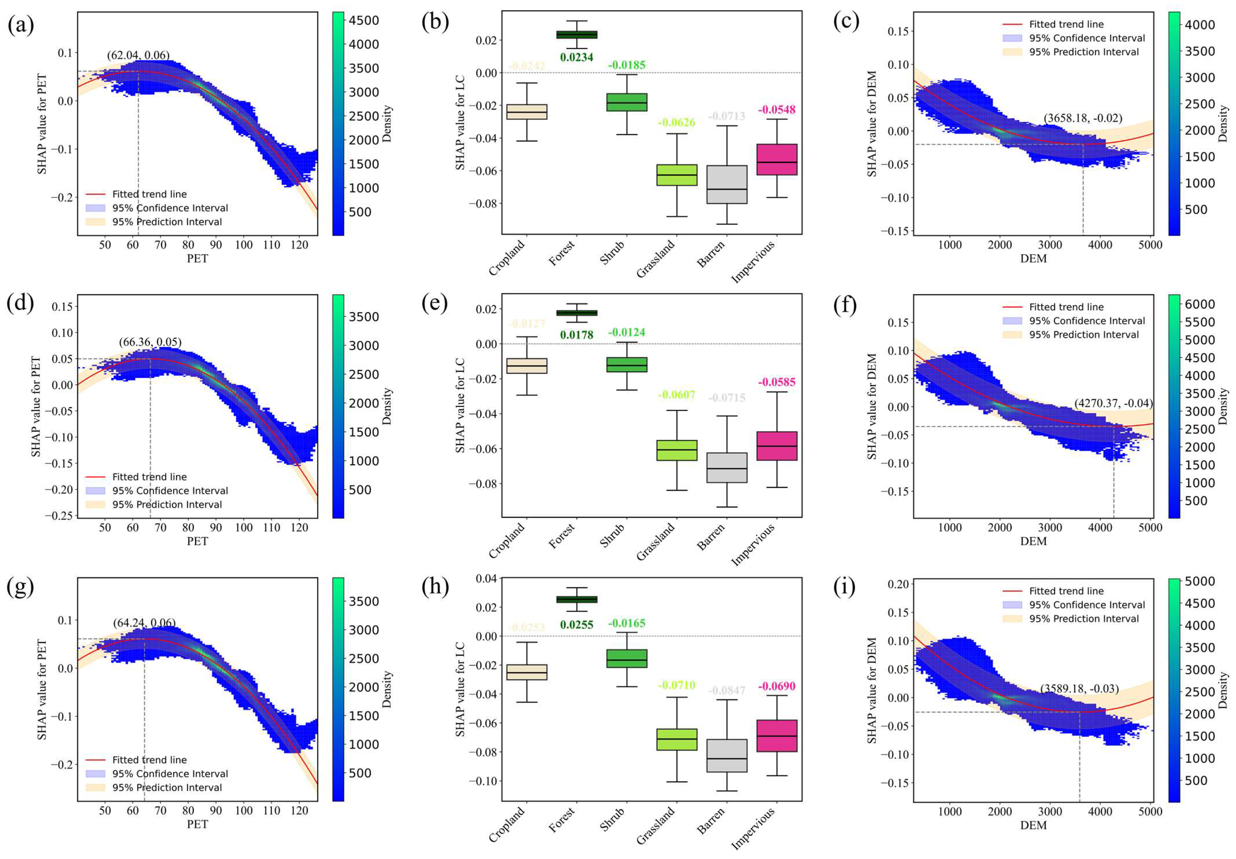
XGBoost-SHAP provides both global and local explanations for individual driving factors. In our study (Figure 11), we plotted dependence plots for the three driving factors with the strongest contributions to RSEI (PET, LC, DEM), quantitatively explaining how changes in each factor affect RSEI. These local explanations are highly effective in developing targeted conservation measures to address specific ecological issues.

(3)

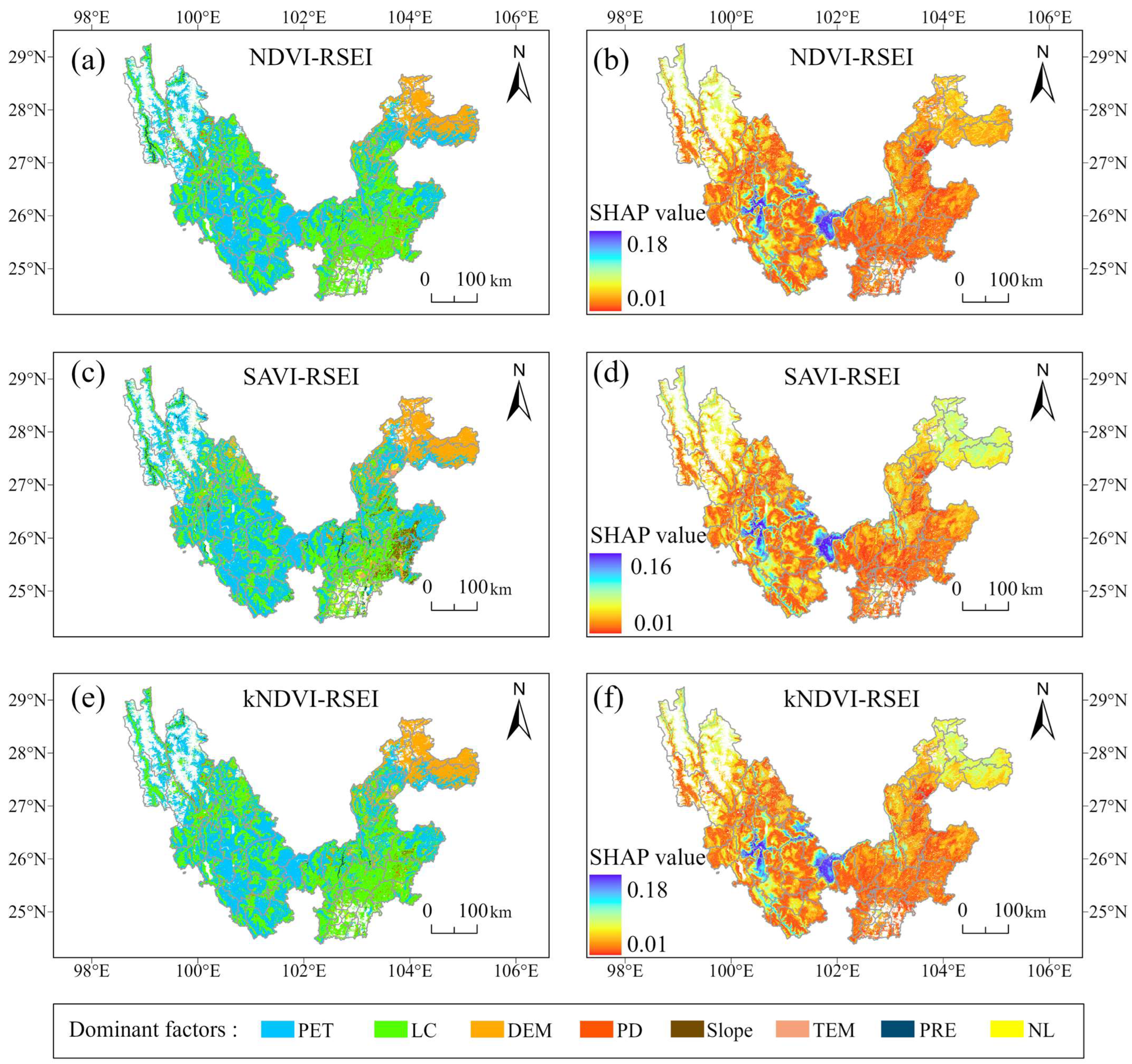
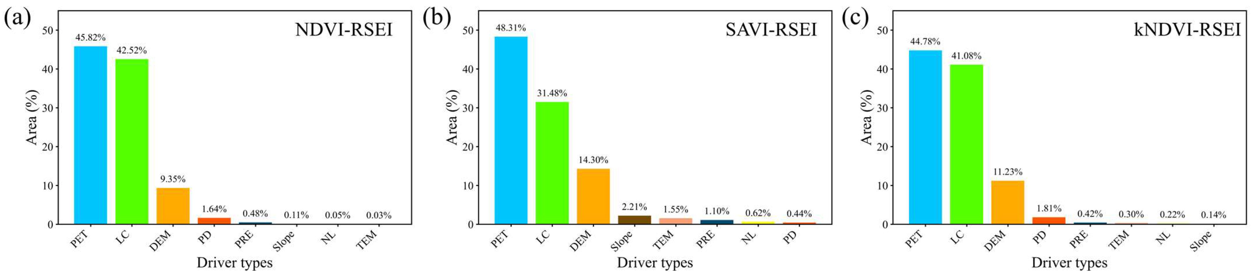
XGBoost-SHAP enables intuitive spatial visualization of model outputs. In our study (Figure 12), we visualized the dominant driving factors for each grid cell of RSEI, facilitating the understanding of complex driving mechanisms from a spatial perspective and translating the results into actionable insights.

This study presents a feasible workflow for using IML to explore the drivers of ecological quality. However, despite the widespread use of IML [30,59], caution is necessary when drawing conclusions. It is essential to carefully evaluate the robustness of the results to ensure the correct application of IML in earth science research.

5. Conclusions

This study evaluated the effectiveness of three different RSEI models, constructed using three greenness indices (NDVI, SAVI, kNDVI), in characterizing watershed ecological quality. The study indicates the following: (1) Compared with the traditional NDVI-constructed RSEI (NDVI-RSEI), the SAVI-RSEI model significantly reduces soil background noise, while the kNDVI-RSEI model simultaneously addresses vegetation saturation in dense canopy areas and exhibits enhanced stability and robustness. (2) Driver factor analysis reveals that RSEI in the northeastern region is primarily influenced by DEM, in the southeastern region by LC, and in the western region by PET. This highlights the spatial heterogeneity of RSEI driving factors and confirms the feasibility of using IML methods such as XGBoost-SHAP to identify ecological quality drivers. Overall, using different greenness indices to calculate ecological quality may introduce biases in RSEI estimation. We recommend carefully considering the spatial heterogeneity of vegetation in the study area when selecting greenness indices for RSEI calculation to better represent the impact of vegetation dynamics on ecological quality.

References

1. Zhou, J.; Liu, W. Monitoring and Evaluation of Eco-Environment Quality Based on Remote Sensing-Based Ecological Index (RSEI) in Taihu Lake Basin, China. Sustainability 2022, 14, 5642. [Google Scholar] [CrossRef]
2. Fan, Y.; Fang, C.; Zhang, Q. Coupling coordinated development between social economy and ecological environment in Chinese provincial capital cities-assessment and policy implications. J. Clean. Prod. 2019, 229, 289–298. [Google Scholar] [CrossRef]
3. Hulme, P.E. Adapting to climate change: Is there scope for ecological management in the face of a global threat? J. Appl. Ecol. 2005, 42, 784–794. [Google Scholar] [CrossRef]
4. Wei, Y.; An, M.; Huang, J.; Fang, X.; Song, M.; Wang, B.; Fan, M.; Wang, X. How human activities affect and reduce ecological sensitivity under climate change: Case study of the Yangtze River Economic Belt, China. J. Clean. Prod. 2024, 472, 143438. [Google Scholar] [CrossRef]
5. Yang, Y.; Chen, S.; Zhou, Y.; Ma, G.; Huang, W.; Zhu, Y. Method for quantitatively assessing the impact of an inter-basin water transfer project on ecological environment-power generation in a water supply region. J. Hydrol. 2023, 618, 129250. [Google Scholar] [CrossRef]
6. Pandey, S.; Kumar, P.; Zlatic, M.; Nautiyal, R.; Panwar, V. Recent advances in assessment of soil erosion vulnerability in a watershed. Int. Soil Water Conserv. Res. 2021, 9, 305–318. [Google Scholar] [CrossRef]
7. Liang, Y.; Liu, L. Simulating land-use change and its effect on biodiversity conservation in a watershed in northwest China. Ecosyst. Health Sustain. 2017, 3, 1335933. [Google Scholar] [CrossRef]
8. Wang, D.; Alimohammadi, N. Responses of annual runoff, evaporation, and storage change to climate variability at the watershed scale. Water Resour. Res. 2012, 48, 2011WR011444. [Google Scholar] [CrossRef]
9. Luck, G.W.; Chan, K.M.A.; Fay, J.P. Protecting ecosystem services and biodiversity in the world’s watersheds. Conserv. Lett. 2009, 2, 179–188. [Google Scholar] [CrossRef]
10. Yuan, Z.; Zhang, W.; Tian, C.; Mao, Y.; Zhou, R.; Wang, H.; Fu, K.; Sun, X. MCRN: A Multi-source Cross-modal Retrieval Network for remote sensing. Int. J. Appl. Earth Obs. Geoinf. 2022, 115, 103071. [Google Scholar] [CrossRef]
11. Sawut, R.; Li, Y.; Kasimu, A.; Ablat, X. Examining the spatially varying effects of climatic and environmental pollution factors on the NDVI based on their spatially heterogeneous relationships in Bohai Rim, China. J. Hydrol. 2023, 617, 128815. [Google Scholar] [CrossRef]
12. Feng, R.; Wang, F.; Wang, K.; Wang, H.; Li, L. Urban ecological land and natural-anthropogenic environment interactively drive surface urban heat island: An urban agglomeration-level study in China. Environ. Int. 2021, 157, 106857. [Google Scholar] [CrossRef]
13. Zhang, Q.; Huang, T.; Xu, S. Assessment of Urban Ecological Resilience Based on PSR Framework in the Pearl River Delta Urban Agglomeration, China. Land 2023, 12, 1089. [Google Scholar] [CrossRef]
14. Nefeslioglu, H.A.; Sezer, E.A.; Gokceoglu, C.; Ayas, Z. A modified analytical hierarchy process (M-AHP) approach for decision support systems in natural hazard assessments. Comput. Geosci. 2013, 59, 1–8. [Google Scholar] [CrossRef]
15. Hu, X.; Xu, H. A new remote sensing index for assessing the spatial heterogeneity in urban ecological quality: A case from Fuzhou City, China. Ecol. Indic. 2018, 89, 11–21. [Google Scholar] [CrossRef]
16. Tang, Q.; Hua, L.; Tang, J.; Jiang, L.; Wang, Q.; Cao, Y.; Wang, T.; Cai, C. Advancing ecological quality assessment in China: Introducing the ARSEI and identifying key regional drivers. Ecol. Indic. 2024, 163, 112109. [Google Scholar] [CrossRef]
17. Cai, C.; Li, J.; Wang, Z. Long-Term Ecological and Environmental Quality Assessment Using an Improved Remote-Sensing Ecological Index (IRSEI): A Case Study of Hangzhou City, China. Land 2024, 13, 1152. [Google Scholar] [CrossRef]
18. Zhang, X.; Wang, X.; Li, W.; Wu, X.; Cheng, X.; Zhou, Z.; Ling, Q.; Liu, Y.; Liu, X.; Hao, J.; et al. Dynamic Monitoring and Analysis of Ecological Environment Quality in Arid and Semi-Arid Areas Based on a Modified Remote Sensing Ecological Index (MRSEI): A Case Study of the Qilian Mountain National Nature Reserve. Remote Sens. 2024, 16, 3530. [Google Scholar] [CrossRef]
19. Yi, S.; Zhou, Y.; Zhang, J.; Li, Q.; Liu, Y.; Guo, Y.; Chen, Y. Spatial-temporal evolution and motivation of ecological vulnerability based on RSEI and GEE in the Jianghan Plain from 2000 to 2020. Front. Environ. Sci. 2023, 11, 1191532. [Google Scholar] [CrossRef]
20. Jiang, Z.; Huete, A.R.; Chen, J.; Chen, Y.; Li, J.; Yan, G.; Zhang, X. Analysis of NDVI and scaled difference vegetation index retrievals of vegetation fraction. Remote Sens. Environ. 2006, 101, 366–378. [Google Scholar] [CrossRef]
21. Huete, A.R.; Liu, H.; Van Leeuwen, W.J.D. The use of vegetation indices in forested regions: Issues of linearity and saturation. In Proceedings of the IGARSS’97, 1997 IEEE International Geoscience and Remote Sensing Symposium Proceedings, Remote Sensing—A Scientific Vision for Sustainable Development, Singapore, 3–8 August 1997; Volume 4. [Google Scholar]
22. Huete, A.R. A soil-adjusted vegetation index (SAVI). Remote Sens. Environ. 1988, 25, 295–309. [Google Scholar] [CrossRef]
23. Camps-Valls, G.; Campos-Taberner, M.; Moreno-Martínez, Á.; Walther, X.; Duveiller, G.; Cescatti, A.; Mahecha, M.; Muñoz-Marí, J.; García-Haro, F.; Guanter, L.; et al. A unified vegetation index for quantifying the terrestrial biosphere. Sci. Adv. 2021, 7, eabc7447. [Google Scholar] [CrossRef] [PubMed]
24. Ma, L.; Yang, B.; Feng, Y.; Ju, L. Evaluation of provincial forest ecological security and analysis of the driving factors in China via the GWR model. Sci. Rep. 2024, 14, 14299. [Google Scholar] [CrossRef]
25. Zhu, X.; Zhang, P.; Wei, Y.; Li, Y.; Zhao, H. Measuring the efficiency and driving factors of urban land use based on the DEA method and the PLS-SEM model—A case study of 35 large and medium-sized cities in China. Sustain. Cities Soc. 2019, 50, 101646. [Google Scholar] [CrossRef]
26. Cai, Z.; Zhang, Z.; Zhao, F.; Guo, X.; Zhao, J.; Xu, Y.; Liu, X. Assessment of eco-environmental quality changes and spatial heterogeneity in the Yellow River Delta based on the remote sensing ecological index and geo-detector model. Ecol. Inform. 2023, 77, 102203. [Google Scholar] [CrossRef]
27. Jiang, S.; Sweet, L.; Blougouras, G.; Brenning, A.; Li, W.; Reichstein, M.; Denzler, J.; Shangguan, W.; Yu, G.; Huang, F.; et al. How Interpretable Machine Learning Can Benefit Process Understanding in the Geosciences. Earth’s Future 2024, 12, e2024EF004540. [Google Scholar] [CrossRef]
28. Chen, T.; Guestrin, C. XGBoost: A Scalable Tree Boosting System. In Proceedings of the 22nd ACM SIGKDD International Conference on Knowledge Discovery and Data Mining, San Francisco, CA, USA, 13–17 August 2016; pp. 785–794. [Google Scholar]
29. Lundberg, S.M.; Lee, S.I. A Unified Approach to Interpreting Model Predictions. In Proceedings of the 31st International Conference on Neural Information Processing Systems, Long Beach, CA, USA, 4–9 December 2017; Volume 30, pp. 4768–4777. [Google Scholar]
30. Xie, J.; Liu, X.; Jasechko, S.; Berghuijs, W.; Wang, K.; Liu, C.; Reichstein, M.; Jung, M.; Koirala, S. Majority of global river flow sustained by groundwater. Nat. Geosci. 2024, 17, 770–777. [Google Scholar] [CrossRef]
31. Yan, Y.; Piao, S.; Hammond, W.M.; Chen, A.; Hong, S.; Xu, H.; Munson, S.M.; Myneni, R.B.; Allen, C.D. Climate-induced tree-mortality pulses are obscured by broad-scale and long-term greening. Nat. Ecol. Evol. 2024, 8, 912–923. [Google Scholar] [CrossRef]
32. Peng, S. 1-km Monthly Precipitation Dataset for China (1901–2023); [DS/OL]; National Tibetan Plateau Data Center: Beijing, China, 2024. [Google Scholar] [CrossRef]
33. Peng, S. 1-km Monthly Mean Temperature Dataset for China (1901–2023); [DS/OL]; National Tibetan Plateau Data Center: Beijing, China, 2024. [Google Scholar] [CrossRef]
34. Peng, S. 1-km Monthly Potential Evapotranspiration Dataset for China (1901–2023); [DS/OL]; National Tibetan Plateau Data Center: Beijing, China, 2024. [Google Scholar] [CrossRef]
35. Wu, Y.; Shi, K.; Chen, Z.; Liu, S.; Chang, Z. An Improved Time-Series DMSP-OLS-Like Data (1992–2023) in China by Integrating DMSP-OLS and SNPP-VIIRS; [DS/OL]; Harvard Dataverse: Cambridge, MA, USA, 2021. [Google Scholar] [CrossRef]
36. Li, J.; Gong, J.; Guldmann, J.M.; Yang, J. Assessment of Urban Ecological Quality and Spatial Heterogeneity Based on Remote Sensing: A Case Study of the Rapid Urbanization of Wuhan City. Remote Sens. 2021, 13, 4440. [Google Scholar] [CrossRef]
37. Maity, S.; Das, S.; Pattanayak, J.M.; Bera, B.; Shit, P.K. Assessment of ecological environment quality in Kolkata urban agglomeration, India. Urban Ecosyst. 2022, 25, 1137–1154. [Google Scholar] [CrossRef]
38. Schultz, M.; Clevers, J.G.P.W.; Carter, S.; Verbesselt, J.; Avitabile, V.; Quang, H.V.; Herold, M. Performance of vegetation indices from Landsat time series in deforestation monitoring. Int. J. Appl. Earth Obs. Geoinf. 2016, 52, 318–327. [Google Scholar] [CrossRef]
39. Ermida, S.L.; Soares, P.; Mantas, V.; Göttsche, F.M.; Trigo, I.F. Google Earth Engine Open-Source Code for Land Surface Temperature Estimation from the Landsat Series. Remote Sens. 2020, 12, 1471. [Google Scholar] [CrossRef]
40. Sen, P.K. Estimates of the Regression Coefficient Based on Kendall’s Tau. J. Am. Stat. Assoc. 1968, 63, 1379–1389. [Google Scholar] [CrossRef]
41. Fernandes, R.; Leblanc, S.G. Parametric (modified least squares) and non-parametric (Theil–Sen) linear regressions for predicting biophysical parameters in the presence of measurement errors. Remote Sens. Environ. 2005, 95, 303–316. [Google Scholar] [CrossRef]
42. Benesty, J.; Chen, J.; Huang, Y.; Cohen, I. Pearson Correlation Coefficient. In Noise Reduction in Speech Processing; Springer Topics in Signal Processing; Springer: Berlin/Heidelberg, Germany, 2009; Volume 2, pp. 1–4. [Google Scholar]
43. Wang, C.; Shen, Y.; Fang, X.; Xiao, S.; Liu, G.; Wang, L.; Gu, B.; Zhou, F.; Chen, D.; Tian, H.; et al. Reducing soil nitrogen losses from fertilizer use in global maize and wheat production. Nat. Geosci. 2024, 17, 1008–1015. [Google Scholar] [CrossRef]
44. Li, J.; Bevacqua, E.; Chen, C.; Wang, Z.; Chen, X.; Myneni, R.B.; Wu, X.; Xu, C.Y.; Zhang, Z.; Zscheischler, J. Regional asymmetry in the response of global vegetation growth to springtime compound climate events. Commun. Earth Environ. 2022, 3, 123. [Google Scholar] [CrossRef]
45. Li, Z. Extracting spatial effects from machine learning model using local interpretation method: An example of SHAP and XGBoost. Comput. Environ. Urban Syst. 2022, 96, 101845. [Google Scholar] [CrossRef]
46. Zhang, X.; Fan, H.; Zhou, C.; Sun, L.; Xu, C.; Lv, T.; Ranagalage, M. Spatiotemporal change in ecological quality and its influencing factors in the Dongjiangyuan region, China. Environ. Sci. Pollut. Res. 2023, 30, 69533–69549. [Google Scholar] [CrossRef]
47. Fisher, J.B.; Whittaker, R.J.; Malhi, Y. ET come home: Potential evapotranspiration in geographical ecology. Glob. Ecol. Biogeogr. 2011, 20, 1–18. [Google Scholar] [CrossRef]
48. Carpenter, C. The environmental control of plant species density on a Himalayan elevation gradient. J. Biogeogr. 2005, 32, 999–1018. [Google Scholar] [CrossRef]
49. Luo, Z.; Sun, Y.; Tang, G.; He, Z.; Peng, L.; Qi, D.; Ou, Z. The Relationship between Reference Crop Evapotranspiration Change Characteristics and Meteorological Factors in Typical Areas of the Middle of the Dry-Hot Valley of Jinsha River. Water 2024, 16, 1512. [Google Scholar] [CrossRef]
50. Deng, R.; Ding, X.; Wang, J. Landscape Ecological Risk Assessmentand Evaluation of Influencing Factors ofJinsha River Basin in Yunnan ProvinceBased on Land Use/Cover Change. Pol. J. Environ. Stud. 2024. [Google Scholar] [CrossRef]
51. Xu, J.; Zheng, L.; Ma, R.; Tian, H. Correlation between Distribution of Rural Settlements and Topography in Plateau-Mountain Area: A Study of Yunnan Province, China. Sustainability 2023, 15, 3458. [Google Scholar] [CrossRef]
52. Deng, Q.; Qin, F.; Zhang, B.; Wang, H.; Luo, M.; Shu, C.; Liu, H.; Liu, G. Characterizing the morphology of gully cross-sections based on PCA: A case of Yuanmou Dry-Hot Valley. Geomorphology 2015, 228, 703–713. [Google Scholar] [CrossRef]
53. Dong, Y.; Xiong, D.; Su, Z.; Li, J.; Yang, D.; Shi, L.; Liu, G. The distribution of and factors influencing the vegetation in a gully in the Dry-hot Valley of southwest China. CATENA 2014, 116, 60–67. [Google Scholar] [CrossRef]
54. Wang, X.; Biederman, J.A.; Knowles, J.F.; Scott, R.L.; Turner, A.J.; Dannenberg, M.P.; Köhler, P.; Frankenberg, G.; Litvak, M.E.; Flerchinger, G.N.; et al. Satellite solar-induced chlorophyll fluorescence and near-infrared reflectance capture complementary aspects of dryland vegetation productivity dynamics. Remote Sens. Environ. 2022, 270, 112858. [Google Scholar] [CrossRef]
55. McDonald, A.J.; Gemmell, F.M.; Lewis, P.E. Investigation of the Utility of Spectral Vegetation Indices for Determining Information on Coniferous Forests. Remote Sens. Environ. 1998, 66, 250–272. [Google Scholar] [CrossRef]
56. Zhang, P.; Liu, H.; Li, H.; Yao, J.; Chen, X.; Feng, J. Using enhanced vegetation index and land surface temperature to reconstruct the solar-induced chlorophyll fluorescence of forests and grasslands across latitude and phenology. Front. For. Glob. Change 2023, 6, 1257287. [Google Scholar] [CrossRef]
57. Barati, S.; Rayegani, B.; Saati, M.; Sharifi, A.; Nasri, M. Comparison the accuracies of different spectral indices for estimation of vegetation cover fraction in sparse vegetated areas. Egypt. J. Remote Sens. Space Sci. 2011, 14, 49–56. [Google Scholar] [CrossRef]
58. Wang, Q.; Moreno-Martínez, Á.; Muñoz-Marí, J.; Campos-Taberner, M.; Camps-Valls, G. Estimation of vegetation traits with kernel NDVI. ISPRS J. Photogramm. Remote Sens. 2023, 195, 408–417. [Google Scholar] [CrossRef]
59. Qin, L.; Zhu, L.; Liu, B.; Li, Z.; Tian, Y.; Mitchell, G.; Shen, S.; Xu, W.; Chen, J. Global expansion of tropical cyclone precipitation footprint. Nat. Commun. 2024, 15, 4824. [Google Scholar] [CrossRef] [PubMed]
Figure 1. The map of the study area. The map of China was made based on the standard map with the drawing review No. GS(2024)-0650, and the base map was not modified.
Land 14 00925 g001
Figure 2. Flowchart of the methodology.
Land 14 00925 g002
Figure 3. XGBoost model performance evaluation result. (a) NDVI-RSEI; (b) SAVI-RSEI; (c) kNDVI-RSEI.
Land 14 00925 g003
Figure 4. Twelve-year average (2000–2022) spatial distributions of mean (a) NDVI-RSEI, (b) SAVI-RSEI, (c) and kNDVI-RSEI. (d) The latitudinal mean of RSEI with a shaded 95% confidence interval. (e) The density distribution of RSEI.
Land 14 00925 g004
Figure 5. Temporal analysis of greenness indices and RSEI from 2000 to 2022.
Land 14 00925 g005
Figure 6. Trend analysis of RSEI from 2000 to 2022. (a) NDVI-RSEI; (b) SAVI-RSEI; (c) kNDVI-RSEI.
Land 14 00925 g006
Figure 7. Spatial distributions of correlations: (a) NDVI with NDVI-RSEI, (b) SAVI with SAVI-RSEI, (c) kNDVI with kNDVI-RSEI; and partial correlations: (d) NDVI with NDVI-RSEI, (e) SAVI with SAVI-RSEI, (f) kNDVI with kNDVI-RSEI. Asterisks (*) indicate statistically significant correlations at p < 0.05.
Land 14 00925 g007
Figure 8. Density distributions of (a) Pearson (b) and Partial correlations between NDVI, SAVI, kNDVI, and their respective RSEI.
Land 14 00925 g008
Figure 9. Image comparisons of greenness and their corresponding RSEI values across six land use types in 2022. Land use types (a), barren (b), grassland (c), forest (d), cropland (e), shrubland (f), and impervious (g).
Land 14 00925 g009
Figure 10. The dependence of RSEI on potential drivers under different greenness. Importance and classification of driving factors for: (a) NDVI-RSEI, (c) SAVI-RSEI, and (e) kNDVI-RSEI; SHAP summary plots (purple numbers represent the absolute SHAP values): (b) NDVI-RSEI, (d) SAVI-RSEI, and (f) kNDVI-RSEI.
Land 14 00925 g010
Figure 11. Relationship between the three most important features and RSEI SHAP value, with distributions of each feature. Dependence plot of PET for (a) NDVI-RSEI, (d) SAVI-RSEI, and (g) kNDVI-RSEI; Dependence plot of LC for (b) NDVI-RSEI, (e) SAVI-RSEI, and (h) kNDVI-RSEI; Dependence plot of DEM for (c) NDVI-RSEI, (f) SAVI-RSEI, and (i) kNDVI-RSEI.
Land 14 00925 g011
Figure 12. The spatial distribution of RSEI driving factors. (a,c,e) The spatial distributions of RSEI dominant factors. (b,d,f) The spatial distributions of SHAP values for RSEI dominant factors.
Land 14 00925 g012
Figure 13. The area proportions of dominant factors for (a) NDVI-RSEI, (b) SAVI-RSEI, and (c) kNDVI-RSEI.
Land 14 00925 g013
Figure 14. The density distribution of SHAP values for dominant factors in the spatial domains of the three RSEI models.
Land 14 00925 g014