Abstract
Mapping ecosystem services (ES) increases the awareness of natural capital value, leading to building sustainability into decision-making processes. Recently, many techniques to assess the value of ES delivered by different scenarios of land use/land cover (LULC) are available, thus becoming important practices in mapping to support the land use planning process. The spatial analysis of the biophysical ES distribution allows a better comprehension of the environmental and social implications of planning, especially when ES concerns the management of risk (e.g., erosion, pollution). This paper investigates the nutrient retention model of InVEST software through its spatial distribution and its quantitative value. The model was analyzed by testing its response to changes in input parameters: (1) the digital terrain elevation model (DEM); and (2) different LULC attribute configurations. The paper increases the level of attention to specific ES models that use water runoff as a proxy of nutrient delivery. It shows that the spatial distribution of biophysical values is highly influenced by many factors, among which the characteristics of the DEM and its interaction with LULC are included. The results seem to confirm that the biophysical value of ES is still affected by a high degree of uncertainty and encourage an expert field campaign as the only solution to use ES mapping for a regulative land use framework.
Keywords:
ecosystem services; mapping; nutrient retention; runoff; urban planning; land use planning 1. Introduction
The interest in understanding the implication of land use changes on different ecosystem services (ES) is garnering attention, using both biophysical and economic values as a proxies of soil degradation [1,2,3,4]. Among others, methodologies for ES accounting at different scales have been developed, and new tools for mapping ES are now available (e.g., Integrated Valuation of Ecosystem Services and Tradeoffs—InVEST, Artificial Intelligence for Ecosystem Services—AIRES, Land Utilization and Capability Indicator—LUCI) [5,6,7,8]. The assessment of ES through their spatial distribution is a key element to set policy targets for sustainability and resiliency because their visualization highlights the trade-off between different alternatives [9,10,11]. Nonetheless, weakness arises when ES mapping is provided at the local scale for regulative planning purposes when the assessment should support the decision-making process regarding land use properties and building rights. In that phase, it seems that the experience of mapping is still in the early stage of development [3,7,12] and the debate on how different methods of mapping ES influence the stakeholder’ s interaction aimed at taking sharp decisions on land use configurations [2,13,14] has not been adequately opened. Few studies have used ES mapping to examine plan goals and objectives [15], even if their explicit integration into planning is, nowadays, crucial to achieving sustainability [16,17,18,19,20].
Such a gap between general ES analysis and its effective implementation at the local stage is underlined by many publications [2,7,13]. The gap is mainly due to a different kind of issue: (i) the ES principles, concepts, and mapping are not yet currently used to define the land use regulation at regional, sub-regional, and local stages [9,21,22,23]; (ii) the technical knowledge of the tools for mapping ES and their utilization during Strategic Environmental Assessments for plans and programs is limited [22,24,25] and; finally, (iii) even when ES are accounted for and considered at the local stage, it is difficult to define how each ES should contribute to achieving an efficient land use plan in terms of the whole, and integrated ecosystem gains rather than of a single function [16,26,27]. Above all considerations, different policy applications require different accuracies, scales, and spatial modeling approaches to set targets and objectives [1,17,22]. Thus, the in-depth comprehension of input-output relations of each ES model became a key point to integrate ES in planning.
The aim of this study is to demonstrate how specific ES values are reliable enough to be used in the decision-making process for land use planning at the local stage. An in-depth assessment of the nutrient retention model defines how the output map is influenced by inputs and, in particular, how the digital terrain elevation model (DEM) affects the delivery of nutrients along the hill slopes in a selected study area. Inasmuch as planners are not experts in the field of ES mapping, the knowledge of model sensitivity to input parameters is essential to create awareness on how critical the use of the output should be when maps are used to set territorial policies rather than land use regulations.
The influence of DEMs with respect to the final output was tested looking at both the spatial distribution of the biophysical value and the quantity of nutrients delivered to the landscape; similarly, the influence of land use/land cover (LULC) data has been tested observing how shifting the load/retain parameters linked to LULC classes affect the output values. After a general analysis, a test of sensitivity has been applied to DEM investigating how different resolutions (10, 20, 25, and 75 m) affect the total export of nutrients in the streams. The behavior of six topographic DEM-related indices have been analyzed selecting a portion of the catchment area characterized by high slopes with a pre-alpine environment and with mountains and hills (the northwestern part of the study area), thus to reduce the time for model processing and obtain a less time-consuming output. A probability distribution has been assigned to DEM variables and the response of the outputs are analyzed.
The results demonstrated how a non-expert utilization of mapping tools should generate possibly distorted evaluations during planning activities. The awareness of how a mapping tool is influenced by inputs is a key element to control the ES mapping process, especially when outputs are used to set planning prescriptions, such as limitation, mitigation, or compensation measures for land use transformations [15].
2. Materials and Methods
2.1. The Research Context
The research LIFE SAM4CP held by the DIST (Interuniversity Department of Regional and Urban Studies and Planning, Politecnico di Torino. DIST is a partner of the LIFE research concerning ES mapping activities. The research group includes the scientific coordinator Prof. Carlo Alberto Barbieri and collaborators Prof. Angioletta Voghera, Prof. Giuseppe Cinà, Prof. Carolina Giaimo, and the technical staff, Francesco Fiermonte, Gabriella Negrini Costanzo Mercugliano, and Marcella Guy) provides a detailed assessment of the spatial distribution of the principal ES using InVEST (Integrated Evaluation of Ecosystem Services and Tradeoffs) [28]. The aim of the research is to carry out the spatial distribution of biophysical values in planning processes, using maps to define an ecological and social assessment of the land use transformations at the local scale and, thus, providing better solutions for communities involved in local planning [11].
The research selected seven ES (habitat quality, carbon sequestration, water yield, nutrient retention, sediment retention, crop pollination, and crop production) to evaluate the sustainability of urban transformations [29,30,31]. InVEST software (InVEST is a suite of free, open-source software models used to map and value the goods and services from nature that sustain and fulfill human life. The software is a product of the partnership between Stanford University and the University of Minnesota, The Nature Conservancy, and the World Wildlife Fund. To download the software, go to: http://www.naturalcapitalproject.org/invest/) [28] is one the primary open access products of the Natural Capital Project, and even if it appears as an easy-to-use software (with on-line training guides) its utilization implies expert knowledge and a collection of numerous amounts of input data (both statistical, with .csv files, and associated geometries with relative raster cell values, rather than vector polygons in .shp format).
The LIFE SAM4CP uses InVEST as the most common and diffuse software to map and assess the biophysical values of the different ES [32,33], nonetheless, the outputs of InVEST were subsequently analyzed in a GIS environment to evaluate the spatial distribution and the quantity of biophysical maps [34,35,36].
When the territorial dimension of the project was defined (municipalities of Bruino, Settimo Torinese, Chieri, and None were selected as the testing areas), then the collection of input data for modeling each ES was setup. The mapping context has been extended to a broad squared selection of Piedmont territory (50 km × 50 km) centered in the pivot city of Turin, thus to avoid the so-called “edge effect” [28] in the testing municipalities (Figure 1). Particularly, the mapping context is a selection of the larger catchment area of the Po River.
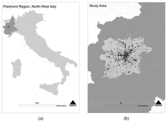
Figure 1.
The context of study. (a) The location of the Piedmont region in Italy and (b) the context of study (in lighter grey, the catchment area).
The mapping context spans 312,525.28 ha and it constitutes 33.8% of the territorial dimension of the metropolitan city of Turin (682,701.11 ha). The selection comprises 26% of plain areas (altitudes below 100 m above sea level (a.s.l.)), 21% of hilly areas (altitudes ranges between 100 and 600 m a.s.l.), and 52% of mountainous area (altitudes above 600 m a.s.l.). Particularly, 17.7% is composed of anthropic areas, 52.7% by agricultural areas, 28.5% by natural and semi-natural zones, and 1.0% by water bodies (Table 1).

Table 1.
Composition of the main land use classes (LULC) in the study area.
The metropolitan area of Turin is composed by a mixed and heterogeneous landscape: from the suburban hills with a semi-dense built-up zone, to the dense and continuous built-up area of the Turin center. The natural mountain zones, and the ones with specific crop management and terraces, to plain floor valleys with a mixed rural development with intensive agricultural productivity, but subjected to high urban expansion. The settlement system of Turin is axially distributed, with a ribbon development along the axes to the northwest (France), northeast (Milan-Venice), and south (Genoa).
After the economic boom in the flat parts of the infrastructural corridors, rather than in the Turin valleys, the pressures of anthropic activities generated a high concentration of land take with the concentration of built-up areas associated with the presence of road networks at the primary and secondary level [37].
2.2. The Planning Outcomes
The nutrient retention model track, with the maximum possible reliability both in terms of geometrical precision and accuracy of the associated biophysical values, is a pixel-based routing of the nutrients that come from diffuse sources in the territory (the composition of the different land uses in the area of investigation) to the delivery areas. When it rains, water flowing over the landscape routes down the slopes carrying pollutants from diffuse sources into streams, rivers, or lakes. Delivery areas are the parts where the water routing model generates a stream, so that the nutrient, which has not been previously retained by the landscape, routes downslope via the surface or subsurface into streams, causing pollution in the streams [28].
Land-use planners need information regarding the contribution of ecosystems to mitigate water pollution. Specifically, they require spatial information on nutrient export and areas where the highest filtration happens. The nutrient retention model provides this information for non-point source pollutants, but it generates a spatially-explicit prefiguration of the areas where pollutants flow into streams; thus, it is possible to reinforce vegetation filtering services to avoid water pollution.
Considering the geometrical resolution of DEMs, many studies found that better model performances are reported in the range of four to 10 m, while coarser pixels generate poor performances [38,39,40]; however, at the same time, it seems that no linear relationship is guaranteed between finer DEM resolution and better reliability, in terms of model output.
As an example, the sediment retention model, which allows calculating the soil erosion, largely depends on the intermediate water routing process that generates the runoff index and, subsequently, additional inputs on land use management interacting with the water flow model. Some cases studies argue that a field campaign after a landslide confirms better feedback with predictive models generated with coarser DEM resolutions.
Analogously, the nutrient retention model consists of a first intermediate process which generates the runoff index which is DEM-dependent, then the results of the intermediate process are used to interact with nutrient loading and absorbing values dependent on LULC. Obviously, if the preliminary interaction with the DEM generates poor performances, then the model increases the errors influencing the final output, which will probably fail to represent a reliable and detailed output usable for decision-making processes.
Mapping nutrient retention is pivotal for the SAM4CP project because the effects of anthropic activities (both for rural and urban uses) on water quality are scarcely used to steer the decision-making process for planning purposes. The standard approach to water pollution control is the reduction of anthropogenic sources in the territory, while it is less considered that the soil has a high power to retain and abate the concentration of pollutants before they reach stream areas.
For instance, if the knowledge of load and retention areas are spatially defined by the nutrient path to streams, the new ecological compensations for urban transformations should consider the plantation of new vegetated areas to increase nutrient removal along the nutrient path, achieving a great result in terms of ecological connectivity, but also in terms of filtering pollutants.
The “filtering” service should be empowered by planning decisions because the vegetation can remove, store, or release the pollutants in other forms. A typical example of the service is provided by the creation of riparian zones. Riparian zones can slow the flows, enabling the removal of pollutants taken up by vegetation and serves as a barrier before pollutants reach the stream. If the knowledge of the nutrient export is spatially represented, then mitigation or compensation measures can be designed by the land use plan as specific contribution to improve the environmental condition of the territory.
Moreover, if biophysical values of the pollutant export are accounted for by the current state and the planned ones, then an in-depth observation of the contaminant trend for alternative land use options should be evaluated. Particularly, the conversion of agricultural land uses, the reduction of natural or semi-natural zones associated with the expansion of urban land uses, represent a threat to water quality. If one of the major targets of contemporary planning is to find sustainable paths for planning transformations, then the trade-off between the land use configuration and the particular variation of different ES should be considered.
Considering the above-mentioned purposes, the research required a technical validation of the nutrient retention model as a key action to understand its direct utilization.
2.3. The Methodology of Validation
In the mapping stage, the spatial distribution of biophysical values for each ES was used as a proxy of soil quality for planning purposes. Such an assessment was necessary since the project was aimed at defining spatial planning rules to limit, mitigate, or compensate for soil sealing [17,41], acting with prescriptive land use regulation [42]. For example, one of the targets was to decide whether or not confirming a potential land use transformation considered the soil ES: if a potential alteration was affecting soils with a high ES provision, then the option of limiting the transformation should be considered, whereas when transformation affects areas of medium ES quality, then different measures of restoration (mitigation or compensation) were promoted [43,44,45].
At that stage, the cause-effect relation between input and output of each single ES model has been verified to avoid mistakes and the potential to distort the evaluations of maps [46,47]. While the spatial distribution of the majority of ES was directly understandable (e.g., habitat quality, carbon sequestration, crop production, crop pollination, and water yield), the nutrient retention and sediment retention models presented a distribution dependent from the DEM, because the final output depends on gravitational models, vegetation, and soil characteristics [34,36,38,40,48,49].
The analytical interpretation of such ES with GIS tools was sometimes counterintuitive and the DIST research team was critical and skeptical about the utilization of models for decision-making processes. Indeed, the process concerning the interpretation of output that determines the design of land use rules has been considered critical.
Considering the above-mentioned perplexities, a period of validation for the nutrient retention model has been planned with the aim of finding accurate relations between input and output; particularly considering the influence of DEM and LULC [50]. Validation consisted of (i) the model being tested by changing the DEM and verifying its effect on the output; and (ii) the output was then used as a benchmark to verify the interaction with LULC.
The methodology of validation considered the analysis of intermediate files as a product of each single model operation. Such an approach was useful to better understand how the model relates the input to the output at each step, increasing the feedback with the final results, and simplified the judgment. Each process was then discussed by the group with technical brainstorming increasing the confidence until a final validation was reached, agreed, and approved.
According to the InVEST users guide [28], the selected inputs for nutrient retention are (see Table A1):
- (1)
- LULC. A GIS raster dataset, with an integer LULC code for each cell.
- (2)
- The analysis has been carried using the Regional Land Cover raster dataset of 2010 (Land Cover Piemonte (LCP)) with a scale of representation of 1:10,000. This dataset is of high utility and precision. Its contents directly fit with the land use classes of the Corine Land Cover Pan-European datasets. Thus, its utilization guarantees a cross-checking analysis of input data between different scales of representation. The LCP has been used as LULC input data for calculation using the selection of the squared territorial borders.
- (3)
- DEM. A GIS raster dataset, with an elevation value for each cell. The DEM should extend beyond the watersheds of interest.
- (4)
- Root restricting layer depth. A GIS raster dataset with an average root restricting layer depth value for each cell.
- (5)
- Precipitation. A GIS raster dataset with the average annual precipitation for each cell.
- (6)
- Plant-available water content. A GIS raster dataset with a plant-available water content value for each cell.
- (7)
- Average annual potential evapotranspiration. A GIS raster dataset, with an annual average evapotranspiration value for each cell.
- (8)
- Watersheds. A shapefile of the watershed polygons.
- (9)
- Biophysical Table. A .csv table of LULC classes containing data on the water quality coefficients used.
Inputs 3 (root restricting layer depth), 4 (precipitation), and 5 (plant-available water content) are dependent to the land capability classification map of Piedmont (Figure 2) which covers the entire catchment area and defines the soil characteristics. The nutrient retention model assumes that nutrients moves towards streams, that the soil is saturated by water (rainfall), and run-off is then generated.
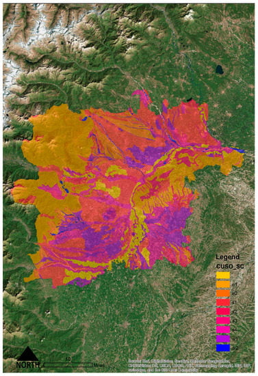
Figure 2.
Land capability classification map used in the study area. Each class is associated to a specific soil characterization.
The distribution of land capability classes is quite heterogeneous in the mapping area. Classes range from 1 (soil suitable for agricultural purposes) to 4 (soil with several limitations to agricultural uses). The soil depth and its composition (the mixture of sand, silt and clay) was a proxy to set the plant-available water content using SPAW software (freely downloadable from the United States Department of Agriculture website) which was needed to set the values of input 6 (Table 2).
Table 2.
Table of input data associated to the Land capability classification map.
3. Results
3.1. Spatial Distribution of Flows and Infiltrations
The model output tracks the path load of a diffuse contaminant (nitrogen, by default), which reaches the stream level from the loading coefficient associated with land use. Accordingly, a sum of per-pixel values in a watershed basin gives, as output, the total amount of pollutants that flow into water streams, affecting the overall water quality. Nitrogen is assumed by the model as the nutrient due to agricultural practices which normally largely affect the water quality at the catchment level. Loading values are concentrated on class 2 (agricultural areas, see Table A1), while retention parameters are distributed in class 3 (natural and semi-natural areas).
The more planned land use changes increase the values of filtering instead of loading and the greater their interaction among the catchment area, the more the absolute nutrient retention value decreases, as a consequence of a better land use composition in the scenario representation.
Interpretation of results comes from an analysis of the “n_export.tif” pixel distribution which represents the biophysical output of the model. The reliability of output, especially for comparative studies between alternative land uses, depends on the interaction between the input data. Even if the DEM sensitivity remains obscure most of the InVEST users, the model generates intermediate folders where each process is placed:
- The model elaborates a water yield calculation based on an evapotranspiration model. This procedure allows the calculation of an intermediate per-pixel representation where the fraction of the rainfall water that is not stored in the soil and removed by evapotranspiration processes moves to another pixel;
- When water is not retained by pixels, the run-off process starts to track the flow-paths that interact with DEM defining the up-flows and stream areas by gravitation. The run-off does not consider if the water routes move via the surface, subsurface, or base flows; it just interacts with the land use model and related nutrient load/retention values. The balance among the load and retention indicates where the landscape contributes to filtering and retaining the nutrients and where nutrients reach the streams.
A preliminary evaluation of the two intermediate results is to check if the runoff model generates the streams in the area where the land use is composed of water bodies. The more streams produced by the runoff model that overlap the water bodies in the land use, the more the results will be reliable in the way the nutrient is routed to the contamination points.
This basilar condition is crucial to set the command “threshold flow accumulation” which defines the number of upstream cells that must flow into a cell before it is considered part of a stream. Indeed, if the model is used at the local scale (1:5,000/1:10,000), then the command has to be set with values ranging from 50 to 200, otherwise it will be sufficient to use values ranging from 500 to 1000 and the correspondence between streams and the water bodies of the large-scale land-use dataset will be achieved.
As explained, DEM is essential to route the flows of nutrients. Its reliability depends on (i) the geometrical definition; and (ii) the continuity and the distribution of the values (holes or gaps to fill in the DEM are frequent).
In the case study, a preliminary observation of the intermediate runoff model has been done using a grid DEM of a 10 m cell (scale of representation, 1:10,000, year 2005) covering the entire territory of the catchment area. It was expected that the flows of water routes down the slopes follow trajectories parallel to gravitational lines, while the model routed the flows with some perpendicular trajectories. Therefore, it has been decided to change the original DEM with an upgraded version which uses a different digital source and presents a denser pixel distribution (which was fundamental to mesh the values among the hill slopes). The geometrical precision of the LULC map was not considered because (i) it did not interact with intermediate phase 1; and (ii) it was precise enough (scale of representation, 1:10,000, year 2010) for the analysis.
The change in the model of the DEM dataset gives important feedback with respect to the new outputs. The changes illustrated in the Figure 3 and Figure 4 show how the interaction with DEM 10 m and DEM 25 m provides a different workflow output (intermediate result after run-off), which implies a better distribution of values.
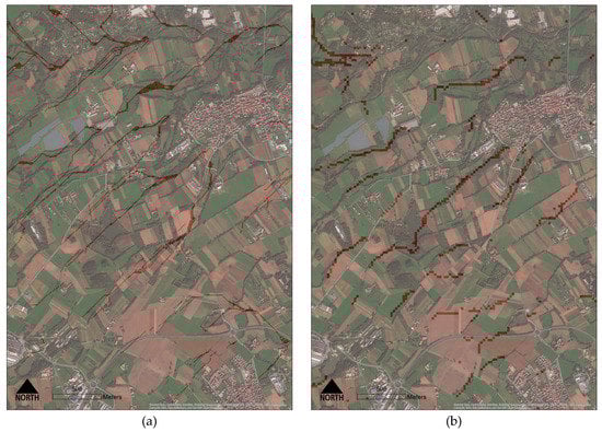
Figure 3.
Correspondence between model streams and the real water bodies. In the left image (a), the runoff model generates streams that are poorly correspondent to the existing watershed (DEM 10 m) while, on the right (b), the model generates streams fairly correspondent to the existing watershed (DEM 25 m).
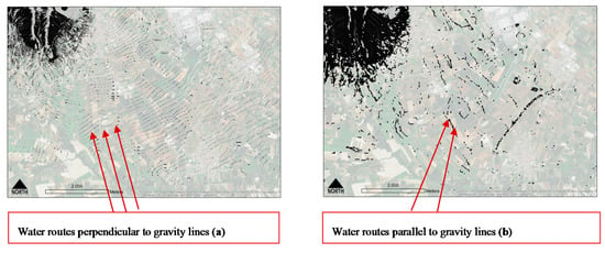
Figure 4.
An example of the different distribution of streams after the intermediate process of runoff. (a) The streams in the model generate mistakes; and (b) the streams in the model correspond to the linear water bodies.
3.2. Model Interaction with DEM and LULC
The correction of the DEM determined a new runoff model which was validated by the group, and the nutrient retention model has been analyzed using its final output instead of the intermediate.
The DEM used in the new version is a product of the official topographical survey of the Piedmont region. It was created between 2000 and 2010 by a grid model of 25 m; thus, the pixel dimension is coarser than the previous DEM used, while the results seem to be more acceptable. The integration of the LULC map with the DEM determines the size of the output grid cells.
The evaluation of the file n_export.tif shows how the integration of the different intermediate results interact together (Figure 5): where the run-off process in upstream areas is intense, then the load of nutrient is higher (particularly when no natural vegetation acts as a filter to the nutrients). In that case, the model shows how pollutants that are not removed by vegetation contaminates the water bodies.
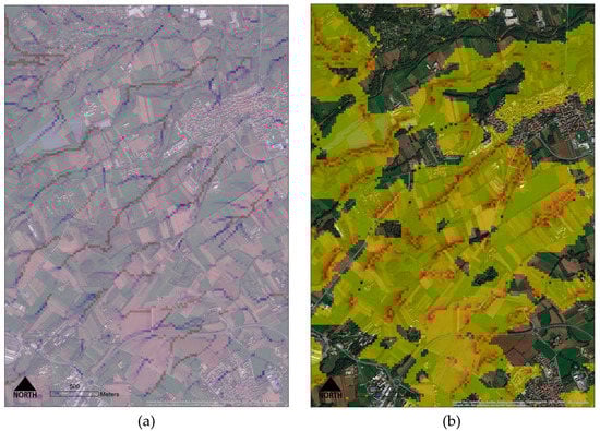
Figure 5.
Areas where the nutrient reaches the streams. (a) The upstream flows (blue) generate the streams (red) while (b) the areas where the nutrient reaches the streams contaminating the water in the catchment are shown.
The use of the 25 m DEM generates a result which was closer to what was expected: the nutrient concentration happened along the buffer areas of rivers, streams, and natural water bodies following a gravitational route and infiltrates where the interaction between the DEM, soil properties, and LULC determines water sinks. Even without a quantitative assessment, the better output distribution is achieved with a coarser DEM resolution, meaning that sometimes the grid resolution does not correspond to a better model output [38]
Once the distribution of the model was spatially acceptable, then a quantitative test was applied to understand how the interaction with LULC properties changes the final result. As introduced, the assessment of the load and retained absolute values of nitrogen associated with each land use type depends on the user. Therefore, to test if the model responds to a different configuration of LULC data, it has been decided to shift the LULC-associated values of the nutrient load with values of retention, thus, obtaining an output which is generated by a different configuration of LULC-dependent variables (Table A2). The result (Table 3) shows a considerably different distribution of nutrients. The interaction between the DEM-dependent block (runoff) and LULC-dependent block (nutrient loads/retain) generates a new map where the contamination process happened from the upstream to the downstream area, but with a different distribution and quantity of values (as expected).
Table 3.
Table of biophysical values in kg of nitrogen at the catchment area. ws_id is the watershed identification number, mn_run_ind is the mean runoff index, n_avl_tot is the total amount of nitrogen in the catchment, n_ret_tot is the total amount of nitrogen retained by the landscape, and n_exp_tot is the total amount of nitrogen exported to the stream in the watershed.
The test confirmed the response of the model to the user modification of input, generating a radically different output.
Considering the “n_exp_tot” is the biophysical output that is considered during the planning process, the differences between the input configurations are outlined by the rows “diff 1–2” and “diff 2–3” (Table 4).
Table 4.
Analysis of DEM indices and output generated by the nutrient retention model (n_exp_tot).
Particularly, the correction of the DEM generates at the catchment scale an absolute augmentation of nitrogen exported to the stream equal to more than 222,658 kg, which corresponds to an augmentation of the previously-registered value of 17.9%. This measure reveals that the DEM quality influences the model workflow and sheds light on the needs of careful use of the input data, assessing both their spatial distribution and their absolute value.
While considering the “diff 2–3”, it is shown that when loading and absorbing values are modified, the net absolute decrease of nitrogen exported to the stream is equal to more than 1,347,448 kg, which implies a reduction of infiltration equal to 91.8%. The decline is due to the LULC conversion which reduces the number of load areas in upslope territories and increases the filtering ones in plain zones; then interaction of runoff with LULC distribution generates an abatement of nitrogen infiltration. That configuration shows a total amount of nitrogen infiltrated of 120,150 kg in the catchment area. The reduction confirms the dependency of output from LULC associated data: the agricultural areas are double the natural and semi-natural ones (121,726.90 ha compared to 65,798.17 ha), therefore, the shift in LULC properties means that the nitrogen loads are halved while the retention areas are doubled. This result seems to confirm good feedback between the quantitative values associated with the input data and their interaction to generate the final output.
The collaboration with external expertise (Dario Masante, Joint Research Centre) confirmed that the intermediate flows of the model were analyzed by other relevant ES software (AIRES of LUCI) [5]. Outputs of the validation process were shared with the external research group, the ones that tested the nutrient retention function with different software to define a comparative assessment.
3.3. Model Sensitivity to DEM
While the feedback from LULC changes was quite intuitive and connected to a linear relationship between the quantity of a particular LULC class and its value of nutrient load or retain, the response of DEM changes still remained less understandable and requested an in-depth analysis.
Four raster DEM datasets were downloaded from different sources (national and regional web geodatabases) and used to see how the nutrient retention output changes in response to DEM substitution (Table 4). To apply the analysis, none of the other input data were changed, in order to obtain an evaluation of the DEM-related dependencies. InVEST runs four times in a sub-area characterized by a hilly and mountainous landscape to reduce the time of elaboration for each result.
The analysis of results has been conducted with a global sensitivity approach on DEM models [51,52] using a probability distribution function assigned to DEM variables. A probability distribution has been founded for DEM indices with an uncertainty degree (linear regression), and outputs were tested against the uncertainty of all input variables. DEM data were thought as a model, and probability distribution functions have been assigned to data variables. The variance between input and output was observed as an indicator of the output’s sensitivity to input changes [53,54].
A global sensitivity analysis was then conducted, with particular attention to:
- Analyze the variation of the model output related to a change in the raster input (DEM). A regression of DEM indices was applied and a simulation of thirteen different DEM configurations and their outputs were tested;
- Analyze the correlation and the variance of each DEM index related to the output; and
- Analyze the dependencies of the DEM input configuration to the nutrient retention output.
Each raster input (DEM) has been evaluated using its related statistical values. In the case study, the value “average” and “standard deviation” were inversely distributed with the DEM resolution.
As shown in Table 4, even if the large majority of indices are inversely proportional to DEM resolution (except minimum and maximum values), their interaction does not generate an output which is inversely related, too. The value of “n_exp_tot” is not linearly distributed according to the geometrical precision of pixels. Instead, the output seems to demonstrate a stochastic distribution. This condition was already explored in other DEM-dependent models (e.g., landslide prediction models, Penna et al. 39) and, what is curious is that (i) the variability of the output is wide, as values ranges from 163,392 kg to 10,398 kg, with a standard deviation of 64,271 kg; and (ii) the lower value (DEM 25) is the one that fits with the real potential distribution of nutrients in the territory, according to an expert-based analysis of the pixel distribution. The geometrical distribution of DEM 25 gives a better feedback compared to others that generate mistakes in the intermediate flow analysis (run-off index distribution).
This means that it is not true that a finer geometrical input resolution in ES models will generate a reliable output. The analysis of the different outputs shows how the change in DEM generates a water-routing intermediate model with different sizes, paths, lengths, and directions of streams in the catchment area with a better approximation to the real streams’ distribution provided by DEM 25.
To have a better analytical assessment of the data, the relation between the model output and DEM input configuration was analyzed with a regression analysis that simulated eleven DEMs and relative outputs. The DEM resolution of simulated values ranged from five to 75 cells, including the four cases studied (Figure 6).
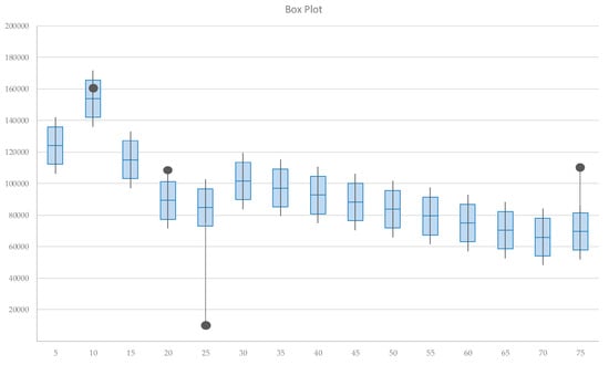
Figure 6.
Box plot of nutrient export simulated values.
Simulations were provided using the index “sum” as the regressor because it showed better correlation to the model output. They confirm that the distribution of the output is nonlinear, and not related to the DEM resolution. The “confidence range” (95th percentile) included the result of the model in just one case (DEM 10) showing, in two cases, an underestimation (DEM 20 and 75) and, in one case, an overestimation (DEM 25). The standard deviation for the simulated models was still high (23,500 kg). The greater deviation is for DEM 25 and, secondly, for DEM 75 (while DEM 20 has a lower deviation).
An in-depth analysis of the values shows that the standard deviation for registered values (model output) and simulated ones remains high (respectively, 64,271.43 and 23,500.93). The confidence range is high, too. Observing how the variance (standard deviation) affects the model output it is possible to test the uncertainty of the input values.
An average influence value for the simulated case is of 26.54%, ranging from 15.27% (DEM 10) to 35.62% (DEM 70). Thus, the variability of the nutrient retention output is affected by a degree of uncertainty dependent on the DEM resolution, which should be considered high (more than 25%, on average).
In conclusion, the interaction of the nutrient retention model with different DEM resolutions is not predictable. Accordingly, it is necessary to have a visual feedback of the pixel output distribution to check how nutrients move toward the landscape.
The variability of the output, which is influenced by the DEM characteristics, is very high, thus an empirical test of the model is highly suggested. In this case, a field study measurement was not considered; nonetheless, to achieve the best input calibration, an empirical survey should be a better solution, with an analysis of the presence of nitrates into the streams in the catchment area.
Even if, for the large majority of users, the DEM resolution is considered a proxy of its reliability (here intended as a good approximation to the real morphological condition of the territory), its interaction with other elements (such as the land use configuration rather than the geological characterization of the soil) is less known and not adequately understood during the use of the InVEST software.
4. Discussion
4.1. Research Limitations and Questions
New models, such as the nutrient retention of InVEST, are helping planners to identify areas where ES are delivered, thus obtaining real progress in the definition of planning dispositions and regulations aimed at increasing the natural capital of the territory [55,56]. Nonetheless, this study sheds light on several important limitations and new questions that arise when a new technology supports the decision-making process for planning purposes. Limitations are important considering the raising awareness of planners or scientists to ES modeling.
The main issues are: (i) the technical limitations in the use of the model; (ii) the restriction in the interpretation of the outputs. With respect to the first, the model has some limitation: (i) it is less applicable to locations where the hydrology is determined by rainfall intensity or in areas where flash rains are predominant; (ii) the model does not address any chemical or biological interactions that may occur from the point of loading to the point of interest; and (iii) the model assumes that there is continuity in the hydraulic flow path [28].
Considering the second issue, even if the study conducted resulted in a better comprehension of the model mechanisms, quantitative outputs are not evaluated by a field campaign of real measures and the model calibration is still incomplete. Such limitations are considerably negative if the model is used to suggest where new environmental compensation measures are finalized to plant new species in buffer areas. If the amount of nitrogen is just indicative than the extension of the buffering system, the selection of species, and the overall biodiversity offset assessment will be complicated [57].
Moreover, the qualitative evaluation of nitrate concentration in open water (50 mg/L, European Directive n. 676 of 12 December 1991), cannot be properly addressed. Despite that, in the near future the model should be tested extending the analysis to the wider ideological catchment area where the basin authority knows the concentrations of nutrients at pre-defined points. In that case, when the user obtains a good preliminary distribution of data, then a better calibration should be achieved.
Nevertheless, it was commonly decided to use the output just as a baseline threshold rather than an absolute value: when an alteration in land use is detected, the model ran a scenario analysis, which should be compared with the original threshold. The rate of change represents the better or worsening delivery of the specific ES.
Finally, one of the major limitations of the nutrient retention model is the complexity of designing each input to meet the data type for the entire catchment area, especially when the model is used, as in the case of SAM4CP research, at the local scale with a fine resolution. Additionally, the temporal resolution of data will affect the response in the catchment to the hydrological integration with respect to land use changes.
4.2. The Integration of the Nutrient Retention Model in Planning Activities
Even if results encourage caution and an in-depth evaluation of results, the utilization of the nutrient retention model help planners to directly identify areas where the vegetation capacity of buffering the contaminants should be improved using compensation measures finalized to abate the nutrient loads, or planting species with a specific characteristic of nutrient drainage. By this point of view, it is hard to find specific rules that directly link the use of the model with a planning prescription.
The significant benefit in applying nutrient retention during the decision-making phase is that all stakeholders involved in planning activity (technicians and politicians) are helped to understand where it is possible to retain more nutrients for different land use configurations. Moreover, the run-off distribution, as well as the flow directions, are important maps because they define the hydrological behavior of the considered landscape under normal conditions.
When all the land use changes are discussed, considering the nutrient retention model, it is possible to address how the changes in soil cover and soil properties increase or decrease the resistance to flow from the surface and, consequently, diminish or augment the nutrient loading in the catchment area. Overall, the results encourage the public administrators and planners to introduce such methodologies into their traditional activities.
Nonetheless, more research is needed because the results reported here show that caution has to be used when preparing input data for an InVEST model that is DEM-dependent. The DEM configuration, associated with land use data, should hardly influence the predictive model of nutrient infiltration, in particular, as the model predictive power is shown to be DEM-configuration dependent.
5. Conclusions
The research conducted shows how it is important to validate quantitative analysis for specific ES in order to overcome the gaps that separate the theoretical framework on ES and its practical application.
Even if at its preliminary stage, the achieved results are encouraging and explain that planners should be aware of how to use techniques of analysis to integrate ES in their valuations. The new locations for ecological compensation zones in the three case studies were selected according to the nutrient retention capacity for specific areas. In particular, the slight reduction of arable land for new natural buffering zones and the selection of land use transformations with the lower environmental impact was supported by the use of InVEST outputs.
Increasing performances of nutrient retention, implies that the future application of planning dispositions will guarantee a better capacity of mitigating the risk of nutrient infiltration in the soil, in the subsoil, and in the water.
Although the traditional procedure for planning and its instruments of evaluation (e.g., the strategic environmental assessment) do not consider ES as quantitative values for measuring the environmental sustainability of plans and programs, the results of the study confirm that a quantification and evaluation of specific ES is, nowadays, possible and welcomed.
Acknowledgments
This study constituted an autonomous work conducted by the DIST group of research involved in the LIFE+ SAM4CP project. The group was supported in the study by Gabriele Garnero (DIST) who is an expert in geomatics and GIS applications for planning. Authors would like to also thank Dario Masante for his valuable feedback on nutrient retention validation procedures and Franco Pellerey for his willingness to work on the sensitivity analysis.
Author Contributions
All authors equally contributed to the article.
Conflicts of Interest
The authors declare no conflict of interest. The founding sponsors had no role in the design of the study; in the collection, analyses, or interpretation of data; in the writing of the manuscript, and in the decision to publish the results.
Appendix A
Table A1.
Table of input data associated to LULC classes.
Table A1.
Table of input data associated to LULC classes.
| LULC | LULC_veg | Root_Dept | kc | Load_n | Load_p | eff_n | eff_p |
|---|---|---|---|---|---|---|---|
| 1111 | 0 | 1 | 0.156122 | 0 | 0 | 0 | 0 |
| 1113 | 0 | 1 | 0.224184 | 0 | 0 | 0 | 0 |
| 1121 | 0 | 1 | 0.287409 | 0 | 0 | 0 | 0 |
| 1123 | 0 | 1 | 0.331544 | 0 | 0 | 0 | 0 |
| 1211 | 0 | 1 | 0.108611 | 0 | 0 | 0 | 0 |
| 1213 | 0 | 1 | 0.1379 | 0 | 0 | 0 | 0 |
| 1221 | 0 | 1 | 0.26101 | 0 | 0 | 0 | 0 |
| 1222 | 0 | 1 | 0.26101 | 0 | 0 | 0 | 0 |
| 1223 | 0 | 1 | 0.108611 | 0 | 0 | 0 | 0 |
| 1230 | 0 | 1 | 0.108611 | 0 | 0 | 0 | 0 |
| 1240 | 0 | 1 | 0.108611 | 0 | 0 | 0 | 0 |
| 1300 | 0 | 1 | 0.100073 | 0 | 0 | 0 | 0 |
| 1310 | 0 | 1 | 0.100073 | 0 | 0 | 0 | 0 |
| 1321 | 0 | 1 | 0.209801 | 0 | 0 | 0 | 0 |
| 1322 | 0 | 1 | 0.507554 | 0 | 0 | 0 | 0 |
| 1331 | 0 | 1 | 0.373765 | 0 | 0 | 0 | 0 |
| 1332 | 0 | 1 | 0.555805 | 0 | 0 | 0 | 0 |
| 1400 | 0 | 550 | 0.448294 | 0 | 0 | 0.6 | 0.6 |
| 1410 | 0 | 550 | 0.522455 | 0 | 0 | 0.6 | 0.6 |
| 1411 | 0 | 550 | 0.489582 | 0 | 0 | 0.6 | 0.6 |
| 1412 | 0 | 550 | 0.546166 | 0 | 0 | 0.6 | 0.6 |
| 1413 | 0 | 1 | 0.110436 | 0 | 0 | 0 | 0 |
| 1421 | 0 | 1 | 0.537704 | 0 | 0 | 0 | 0 |
| 1422 | 0 | 1 | 0.537704 | 0 | 0 | 0 | 0 |
| 1423 | 0 | 1 | 0.537704 | 0 | 0 | 0 | 0 |
| 2000 | 1 | 675 | 0.483 | 210 | 80 | 0.4 | 0.4 |
| 2101 | 1 | 675 | 0.483 | 210 | 80 | 0.4 | 0.4 |
| 2102 | 1 | 675 | 0.483 | 210 | 80 | 0.4 | 0.4 |
| 2103 | 1 | 675 | 0.483 | 210 | 80 | 0.4 | 0.4 |
| 2104 | 1 | 675 | 0.483 | 210 | 80 | 0.4 | 0.4 |
| 2111 | 1 | 675 | 0.483 | 210 | 80 | 0.4 | 0.4 |
| 2112 | 1 | 675 | 0.483 | 210 | 80 | 0.4 | 0.4 |
| 2113 | 1 | 675 | 0.483 | 210 | 80 | 0.4 | 0.4 |
| 2114 | 1 | 675 | 0.483 | 210 | 80 | 0.4 | 0.4 |
| 2121 | 1 | 675 | 0.483 | 210 | 80 | 0.4 | 0.4 |
| 2122 | 1 | 675 | 0.483 | 210 | 80 | 0.4 | 0.4 |
| 2123 | 1 | 675 | 0.483 | 210 | 80 | 0.4 | 0.4 |
| 2124 | 1 | 675 | 0.483 | 210 | 80 | 0.4 | 0.4 |
| 2130 | 1 | 800 | 0.616 | 275 | 100 | 0.4 | 0.4 |
| 2200 | 1 | 1500 | 0.7 | 0 | 0 | 0.6 | 0.6 |
| 2210 | 1 | 1500 | 0.4 | 76 | 44 | 0.4 | 0.4 |
| 2220 | 1 | 1200 | 0.75 | 85 | 55 | 0.4 | 0.4 |
| 2221 | 1 | 1200 | 0.75 | 85 | 55 | 0.4 | 0.4 |
| 2222 | 1 | 1200 | 0.75 | 85 | 55 | 0.4 | 0.4 |
| 2223 | 1 | 1200 | 0.75 | 85 | 55 | 0.4 | 0.4 |
| 2224 | 1 | 1200 | 0.75 | 85 | 55 | 0.4 | 0.4 |
| 2225 | 1 | 1200 | 0.75 | 85 | 55 | 0.4 | 0.4 |
| 2230 | 1 | 1400 | 0.6 | 200 | 150 | 0.4 | 0.4 |
| 2240 | 1 | 1500 | 0.7 | 0 | 0 | 0.6 | 0.6 |
| 2241 | 1 | 1500 | 0.7 | 0 | 0 | 0.6 | 0.6 |
| 2310 | 1 | 550 | 0.72 | 0 | 0 | 0.6 | 0.6 |
| 2410 | 1 | 1500 | 0.7 | 0 | 0 | 0.6 | 0.6 |
| 2420 | 1 | 675 | 0.483 | 210 | 80 | 0.4 | 0.4 |
| 2430 | 1 | 800 | 0.72 | 30 | 90 | 0.4 | 0.4 |
| 2440 | 1 | 800 | 0.72 | 30 | 90 | 0.4 | 0.4 |
| 3110 | 1 | 1500 | 0.7 | 0 | 0 | 0.8 | 0.8 |
| 3111 | 1 | 1500 | 0.7 | 0 | 0 | 0.8 | 0.8 |
| 3112 | 1 | 1500 | 0.7 | 0 | 0 | 0.8 | 0.8 |
| 3113 | 1 | 1500 | 0.7 | 0 | 0 | 0.8 | 0.8 |
| 3114 | 1 | 1500 | 0.7 | 0 | 0 | 0.8 | 0.8 |
| 3115 | 1 | 1500 | 0.7 | 0 | 0 | 0.8 | 0.8 |
| 3116 | 1 | 1500 | 0.7 | 0 | 0 | 0.8 | 0.8 |
| 3117 | 1 | 1500 | 0.7 | 0 | 0 | 0.8 | 0.8 |
| 3118 | 1 | 1500 | 0.7 | 0 | 0 | 0.8 | 0.8 |
| 3119 | 1 | 1500 | 0.7 | 0 | 0 | 0.8 | 0.8 |
| 3120 | 1 | 1500 | 0.7 | 0 | 0 | 0.8 | 0.8 |
| 3121 | 1 | 1500 | 0.7 | 0 | 0 | 0.8 | 0.8 |
| 3122 | 1 | 1500 | 0.7 | 0 | 0 | 0.8 | 0.8 |
| 3123 | 1 | 1500 | 0.7 | 0 | 0 | 0.8 | 0.8 |
| 3124 | 1 | 1500 | 0.7 | 0 | 0 | 0.8 | 0.8 |
| 3130 | 1 | 1500 | 0.7 | 0 | 0 | 0.8 | 0.8 |
| 3210 | 1 | 550 | 0.72 | 0 | 0 | 0.6 | 0.6 |
| 3220 | 1 | 550 | 0.72 | 0 | 0 | 0.6 | 0.6 |
| 3230 | 1 | 550 | 0.72 | 0 | 0 | 0.6 | 0.6 |
| 3240 | 1 | 550 | 0.72 | 0 | 0 | 0.6 | 0.6 |
| 3241 | 1 | 550 | 0.72 | 0 | 0 | 0.6 | 0.6 |
| 3300 | 1 | 1 | 0 | 0 | 0 | 0.6 | 0.6 |
| 3310 | 1 | 1 | 0 | 0 | 0 | 0.6 | 0.6 |
| 3320 | 1 | 1 | 0 | 0 | 0 | 0.6 | 0.6 |
| 3330 | 1 | 1 | 0 | 0 | 0 | 0.6 | 0.6 |
| 3340 | 1 | 1 | 0 | 0 | 0 | 0.6 | 0.6 |
| 3350 | 1 | 1 | 0 | 0 | 0 | 0.6 | 0.6 |
| 4100 | 1 | 0 | 0 | 0 | 0 | 0 | 0 |
| 4110 | 1 | 0 | 0 | 0 | 0 | 0 | 0 |
| 4120 | 1 | 0 | 0 | 0 | 0 | 0 | 0 |
| 5110 | 1 | 0 | 0 | 0 | 0 | 0 | 0 |
| 5111 | 1 | 0 | 0 | 0 | 0 | 0 | 0 |
| 5112 | 1 | 0 | 0 | 0 | 0 | 0 | 0 |
| 5120 | 1 | 0 | 0 | 0 | 0 | 0 | 0 |
| 5121 | 1 | 0 | 0 | 0 | 0 | 0 | 0 |
| 5122 | 1 | 0 | 0 | 0 | 0 | 0 | 0 |
| 5123 | 1 | 0 | 0 | 0 | 0 | 0 | 0 |
Table A2.
Validation of the model changing LULC code attributes.
Table A2.
Validation of the model changing LULC code attributes.
| DN Code | Description | LULC | LULC Modified |
|---|---|---|---|
| 70 | Continuous and dense built-up areas | 1111 | 1111 |
| 72 | Continuous and semi-dense built-up areas | 1113 | 1113 |
| 74 | Discontinuous built-up areas | 1121 | 1121 |
| 76 | Sparse built-up areas | 1123 | 1123 |
| 78 | Continuous and dense industrial, commercial and service zones | 1211 | 1211 |
| 80 | Discontinuous industrial, commercial and service zones | 1213 | 1213 |
| 82 | Road network | 1221 | 1221 |
| 83 | Railway network | 1222 | 1222 |
| 86 | Airports | 1240 | 1240 |
| 87 | Exctration, dumps and construction sites | 1300 | 1300 |
| 89 | Quarries and mines | 1321 | 1321 |
| 93 | Green non agricultural artificial areas | 1400 | 1400 |
| 97 | Cemetries | 1413 | 1413 |
| 99 | Sport plans | 1422 | 1422 |
| 101 | Indifferentiate agricultural land | 2000 | 3110 |
| 102 | Indifferentiate crops | 2101 | 3111 |
| 103 | Indifferentiate vivarium | 2102 | 3112 |
| 104 | Indifferentiate ortyards | 2103 | 3113 |
| 105 | Indifferentiated greenhouses | 2104 | 3114 |
| 106 | Non irrigated crops | 2111 | 3115 |
| 110 | Irrigated crops | 2121 | 3116 |
| 114 | Rise | 2130 | 3118 |
| 115 | Permanent crops | 2200 | 3119 |
| 116 | Vines | 2210 | 3120 |
| 117 | Indifferentiated fruits | 2220 | 3121 |
| 118 | Hazel | 2221 | 3122 |
| 119 | Chestnut | 2222 | 3124 |
| 120 | Apple orchards | 2223 | 3130 |
| 121 | Peach orchards | 2224 | 3210 |
| 122 | Kiwi plants | 2225 | 3220 |
| 123 | Olive groves | 2230 | 3240 |
| 124 | Wood arboriculture | 2240 | 3300 |
| 125 | Poplars | 2241 | 3310 |
| 126 | Grasslands and pastures | 2310 | 3320 |
| 129 | Agricultural land mixed with natural areas | 2430 | 3330 |
| 131 | Broadleaf forest | 3110 | 2000 |
| 132 | Maple-limes | 3111 | 2101 |
| 133 | Chestnuts | 3112 | 2102 |
| 134 | Locust trees | 3113 | 2103 |
| 135 | Hornbeams | 3114 | 2104 |
| 136 | Oak trees | 3115 | 2111 |
| 137 | Downy oak | 3116 | 2121 |
| 139 | Beeches | 3118 | 2130 |
| 141 | Riparian vegetation | 3120 | 2210 |
| 142 | Firs forests | 3121 | 2220 |
| 143 | Pine forests | 3122 | 2221 |
| 145 | Larch forests | 3124 | 2222 |
| 146 | Mixed broadleaf and coniferous forests | 3130 | 2223 |
| 147 | Mountain prairies and moorlands | 3210 | 2224 |
| 148 | Shrublands | 3220 | 2225 |
| 150 | Transitional woodlands and shrublands | 3240 | 2230 |
| 152 | Barelands | 3300 | 2240 |
| 153 | Sand | 3310 | 2241 |
| 154 | Bare rocks | 3320 | 2310 |
| 155 | Sparse vegetation | 3330 | 2430 |
| 156 | Burnt areas | 3340 | 3340 |
| 159 | Sweamps | 4110 | 4110 |
| 160 | Peatlands | 4120 | 4120 |
| 162 | Rivers and creeks | 5111 | 5111 |
| 163 | Canals | 5112 | 5112 |
| 164 | Water basins | 5120 | 5120 |
| 165 | Natural water basins | 5121 | 5121 |
| 166 | Artificial water basins | 5122 | 5122 |
References
- Schröter, M.; Remme, R.P.; Sumarga, E.; Barton, D.N.; Hein, L. Lessons learned for spatial modelling of ecosystem services in support of ecosystem accounting. Ecosyst. Serv. 2014, 13, 64–69. [Google Scholar] [CrossRef]
- Lavorel, S.; Bayer, A.; Bondeau, A.; Lautenbach, S.; Ruiz-Frau, A.; Schulp, N.; Seppelt, R.; Verburg, P.; Teeffelen, A.; Vannier, C.; et al. Pathways to bridge the biophysical realism gap in ecosystem services mapping approaches. Ecol. Indic. 2017, 74, 241–260. [Google Scholar] [CrossRef]
- Crossman, N.D.; Burkhard, B.; Nedkov, S.; Willemen, L.; Petz, K.; Palomo, I.; Drakou, E.G.; Martín-Lopez, B.; McPhearson, T.; Boyanova, K.; et al. A blueprint for mapping and modelling ecosystem services. Ecosyst. Serv. 2013, 4, 4–14. [Google Scholar] [CrossRef]
- Mononen, L.; Auvinen, A.P.; Ahokumpu, A.L.; Rönkä, M.; Aarras, N.; Tolvanen, H.; Kamppinen, M.; Viirret, E.; Kumpula, T.; Vihervaara, P. National ecosystem service indicators: Measures of social-ecological sustainability. Ecol. Indic. 2016, 61, 21–37. [Google Scholar] [CrossRef]
- Sharps, K.; Masante, D.; Thomas, A.; Jackson, B.; Redhead, J.; May, L.; Prosser, H.; Cosby, B.; Emmett, B.; Jones, L. Comparing strengths and weaknesses of three ecosystem services modelling tools in a diverse UK river catchment. Sci. Total Environ. 2017, 584, 118–130. [Google Scholar] [CrossRef] [PubMed]
- Naidoo, R.; Balmford, A.; Costanza, R.; Fisher, B.; Green, R.E.; Lehner, B.; Malcolm, T.R.; Ricketts, T.H. Global mapping of ecosystem services and conservation priorities. Proc. Natl. Acad. Sci. USA. 2008, 105, 9495–9500. [Google Scholar] [CrossRef] [PubMed]
- Maes, J.; Egoh, B.; Willemen, L.; Liquete, C.; Vihervaara, P.; Schägner, J.P.; Grizzetti, B.; Drakou, E.G.; Notte, A.L.; Zulian, G.; et al. Mapping ecosystem services for policy support and decision making in the European Union. Ecosyst. Serv. 2012, 1, 31–39. [Google Scholar] [CrossRef]
- Salata, S.; Ronchi, S.; Arcidiacono, A.; Ghirardelli, F. Mapping Habitat Quality in the Lombardy Region, Italy. One Ecosyst. 2017, 2, e11402. [Google Scholar]
- Wong, C.P.; Jiang, B.; Kinzig, A.P.; Lee, K.N.; Ouyang, Z. Linking ecosystem characteristics to final ecosystem services for public policy. Ecol. Lett. 2015, 18, 108–118. [Google Scholar] [CrossRef] [PubMed]
- Artmann, M. Urban gray vs. urban green vs. soil protection-Development of a systemic solution to soil sealing management on the example of Germany. Environ. Impact Assess. Rev. 2016, 59, 27–42. [Google Scholar] [CrossRef]
- Giaimo, C.; Regis, D.; Salata, S. Integrated Process of Ecosystem Services Evaluation and Urban Planning. The Experience of LIFE SAM4CP Project towards Sustainable and Smart Communities; Bertoldi, P., Ed.; European Union: Frankfurt, Germany, 2016; pp. 43–54. [Google Scholar]
- Batista e Silva, F.; Lavalle, C.; Jacobs-Crisioni, C.; Barranco, R.; Zulian, G.; Maes, J.; Baranzelli, C.; Castillo, C.P.; Vandecasteele, I.; Ustaoglu, E.; et al. Direct and Indirect Land Use Impacts of the EU Cohesion Policy Assessment with the Land Use Modelling Platform Contact information; European Union: Luxembourg, 2013. [Google Scholar]
- Langemeyer, J.; Gómez-Baggethun, E.; Haase, D.; Scheuer, S.; Elmqvist, T. Bridging the gap between ecosystem service assessments and land-use planning through Multi-Criteria Decision Analysis (MCDA). Environ. Sci. Policy 2016, 62, 45–56. [Google Scholar] [CrossRef]
- Hilde, T.; Paterson, R. Integrating ecosystem services analysis into scenario planning practice: Accounting for street tree benefits with i-Tree valuation in Central Texas. J. Environ. Manag. 2014, 146, 524–534. [Google Scholar] [CrossRef] [PubMed]
- Woodruff, S.C.; BenDor, T.K. Ecosystem services in urban planning: Comparative paradigms and guidelines for high quality plans. Landsc. Urban Plan. 2016, 152, 90–100. [Google Scholar] [CrossRef]
- Kabisch, N. Ecosystem service implementation and governance challenges in urban green space planning—The case of Berlin, Germany. Land Use Policy 2015, 42, 557–567. [Google Scholar] [CrossRef]
- Hayek, U.W.; Teich, M.; Klein, T.M.; Grêt-Regamey, A. Bringing ecosystem services indicators into spatial planning practice: Lessons from collaborative development of a web-based visualization platform. Ecol. Indic. 2016, 61, 90–99. [Google Scholar] [CrossRef]
- Baró, F.; Palomo, I.; Zulian, G.; Vizcaino, P.; Haase, D.; Gómez-Baggethun, E. Mapping ecosystem service capacity, flow and demand for landscape and urban planning: A case study in the Barcelona metropolitan region. Land Use Policy 2016, 57, 405–417. [Google Scholar] [CrossRef]
- Primmer, E.; Furman, E. Operationalising ecosystem service approaches for governance: Do measuring, mapping and valuing integrate sector-specific knowledge systems? Ecosyst. Serv. 2012, 1, 85–92. [Google Scholar] [CrossRef]
- Bateman, I.J.; Harwood, A.R.; Mace, G.M.; Watson, R.T.; Abson, D.J.; Andrews, B.; Binner, A.; Crowe, A.; Day, B.H.; Dugdale, S.; et al. Bringing ecosystem services into economic decision-making: Land use in the United Kingdom. Science 2013, 341, 45–50. [Google Scholar] [CrossRef] [PubMed]
- Wallace, K.J. Classification of ecosystem services: Problems and solutions. Biol. Conserv. 2007, 139, 235–246. [Google Scholar] [CrossRef]
- Baker, J.; Sheate, W.R.; Phillips, P.; Eales, R. Ecosystem services in environmental assessment—Help or hindrance? Environ. Impact Assess. Rev. 2013, 40, 3–13. [Google Scholar] [CrossRef]
- Arcidiacono, A.; Ronchi, S.; Salata, S. Ecosystem services assessment using invest as a tool to support decision making process: Critical issues and opportunities. Int. Conf. Comput. Sci. Appl. 2015, 9158, 35–49. [Google Scholar]
- Partidario, M.R.; Gomes, R.C. Ecosystem services inclusive strategic environmental assessment. Environ. Impact Assess. Rev. 2013, 40, 36–46. [Google Scholar] [CrossRef]
- Mascarenhas, A.; Ramos, T.B.; Haase, D.; Santos, R. Ecosystem services in spatial planning and strategic environmental assessment-A European and Portuguese profile. Land Use Policy 2015, 48, 158–169. [Google Scholar] [CrossRef]
- La Rosa, D.; Barbarossa, L.; Privitera, R.; Martinico, F. Agriculture and the city: A method for sustainable planning of new forms of agriculture in urban contexts. Land Use Policy 2014, 41, 290–303. [Google Scholar] [CrossRef]
- Geneletti, D. Assessing the impact of alternative land-use zoning policies on future ecosystem services. Environ. Impact Assess. Rev. 2012, 40, 25–35. [Google Scholar] [CrossRef]
- Sharp, E.R.; Chaplin-kramer, R.; Wood, S.; Guerry, A.; Tallis, H.; Ricketts, T.; Authors, C.; Nelson, E.; Ennaanay, D.; Wolny, S.; et al. InVEST User’s Guide 2016. Available online: https://www.naturalcapitalproject.org/invest/ (accessed on 16 May 2017).
- Potschin, M.; Haines-Young, R. Landscapes, sustainability and the place-based analysis of ecosystem services. Landsc. Ecol. 2013, 28, 1053–1065. [Google Scholar] [CrossRef]
- Laprise, M.; Lufkin, S.; Rey, E. An indicator system for the assessment of sustainability integrated into the project dynamics of regeneration of disused urban areas. Build. Environ. 2015, 86, 29–38. [Google Scholar] [CrossRef]
- Elmqvist, T.; Setälä, H.; Handel, S.N.; van der Ploeg, S.; Aronson, J.; Blignaut, J.N.; Gómez-Baggethun, E.; Nowak, D.J.; Kronenberg, J.; de Groot, R. Benefits of restoring ecosystem services in urban areas. Curr. Opin. Environ. Sustain. 2015, 14, 101–108. [Google Scholar] [CrossRef]
- Keller, A.A.; Fournier, E.; Fox, J. Minimizing impacts of land use change on ecosystem services using multi-criteria heuristic analysis. J. Environ. Manag. 2015, 156, 23–30. [Google Scholar] [CrossRef] [PubMed]
- Goldstein, J.H.; Caldarone, G.; Duarte, T.K.; Ennaanay, D.; Hannahs, N.; Mendoza, G.; Polasky, S.; Wolny, S.; Daily, G.C. Integrating ecosystem-service tradeoffs into land-use decisions. Proc. Natl. Acad. Sci. USA 2012, 109, 7565–7570. [Google Scholar] [CrossRef] [PubMed]
- Aiello, A.; Adamo, M.; Canora, F. Remote sensing and GIS to assess soil erosion with RUSLE3D and USPED at river basin scale in southern Italy. CATENA 2015, 131, 174–185. [Google Scholar] [CrossRef]
- Siedentop, S.; Fina, S. Monitoring urban sprawl in Germany: Towards a GIS-based measurement and assessment approach. J. Land Use Sci. 2010, 5, 73–104. [Google Scholar] [CrossRef]
- Ganasri, B.P.; Ramesh, H. Assessment of soil erosion by RUSLE model using remote sensing and GIS—A case study of Nethravathi Basin. Geosci. Front. 2016, 7, 953–961. [Google Scholar] [CrossRef]
- Cassatella, C. The “Corona Verde” Strategic Plan: An integrated vision for protecting and enhancing the natural and cultural heritage. Urban Res. Pract. 2013, 6, 219–228. [Google Scholar] [CrossRef]
- Penna, D.; Borga, M.; Aronica, G.T.; Brigandì, G.; Tarolli, P. The influence of grid resolution on the prediction of natural and road-related shallow landslides. Hydrol. Earth Syst. Sci. 2014, 18, 2127–2139. [Google Scholar] [CrossRef]
- Maleika, W. The influence of the grid resolution on the accuracy of the digital terrain model used in seabed modeling. Mar. Geophys. Res. 2015, 36, 35–44. [Google Scholar] [CrossRef]
- Prasuhn, V.; Liniger, H.; Gisler, S.; Herweg, K.; Candinas, A.; Clément, J.P. A high-resolution soil erosion risk map of Switzerland as strategic policy support system. Land Use Policy 2013, 32, 281–291. [Google Scholar] [CrossRef]
- Orgiazzi, A.; Panagos, P.; Yigini, Y.; Dunbar, M.B.; Gardi, C.; Montanarella, L.; Ballabio, C. A knowledge-based approach to estimating the magnitude and spatial patterns of potential threats to soil biodiversity. Sci. Total Environ. 2016, 545, 11–20. [Google Scholar] [CrossRef] [PubMed]
- Arcidiacono, A.; Ronchi, S.; Salata, S. Managing Multiple Ecosystem Services for Landscape Conservation: A Green Infrastructure in Lombardy Region. Proc. Eng. 2016, 161, 2297–2303. [Google Scholar] [CrossRef]
- European Commission. Mapping and Assessment of Ecosystems and Their Services; European Commission: Luxembourg, 2016. [Google Scholar]
- Zoppi, C.; Lai, S. Land-taking processes: An interpretive study concerning an Italian region. Land Use Policy 2014, 36, 369–380. [Google Scholar] [CrossRef]
- Barbosa, A.; Vallecillo, S.; Baranzelli, C.; Jacobs-Crisioni, C.; Batista e Silva, F.; Perpiña-Castillo, C.; Lavalle, C.; Maes, J. Modelling built-up land take in Europe to 2020: An assessment of the Resource Efficiency Roadmap measure on land. J. Environ. Plan. Manag. 2016, 60, 1439–1463. [Google Scholar] [CrossRef]
- Elliff, C.I.; Kikuchi, R.K.P. The ecosystem service approach and its application as a tool for integrated coastal management. Nat. Conserv. 2015, 13, 105–111. [Google Scholar] [CrossRef]
- Boyd, J.; Banzhaf, S. What are ecosystem services? The need for standardized environmental accounting units. Ecol. Econ. 2007, 63, 616–626. [Google Scholar] [CrossRef]
- Ryan, J.; McAlpine, C.; Ludwig, J.; Callow, J. Modelling the Potential of Integrated Vegetation Bands (IVB) to Retain Stormwater Runoff on Steep Hillslopes of Southeast Queensland, Australia. Land 2015, 4, 711–736. [Google Scholar] [CrossRef]
- Prasannakumar, V.; Vijith, H.; Abinod, S.; Geetha, N. Estimation of soil erosion risk within a small mountainous sub-watershed in Kerala, India, using Revised Universal Soil Loss Equation (RUSLE) and geo-information technology. Geosci. Front. 2012, 3, 209–215. [Google Scholar] [CrossRef]
- Godone, D.; Garnero, G. The role of morphometric parameters in Digital Terrain Models interpolation accuracy: A case study. Eur. J. Remote Sens. 2013, 46, 198–214. [Google Scholar] [CrossRef]
- Saltelli, A. Sensitivity Analysis: An Introduction. Available online: http://www.andreasaltelli.eu/file/repository/Saltelli_Lesson_Sens_Analysis_3.pdf (accessed on 16 May 2017).
- Van Griensven, A.; Meixner, T.; Grunwald, S.; Bishop, T.; Diluzio, M.; Srinivasan, R. A global sensitivity analysis tool for the parameters of multi-variable catchment models. J. Hydrol. 2006, 324, 10–23. [Google Scholar] [CrossRef]
- Iooss, B.; Lemaître, P. A review on global sensitivity analysis methods. Uncertain. Manag. Simul. Optim. Complex Syst. 2014, 59, 101–122. [Google Scholar]
- Muñoz-Carpena, R.; Zajac, Z.; Kuo, Y. Global sensitivity and uncertainty analyses of the water quality model VFSMOD-W. Trans. ASABE 2007, 50, 1719–1732. [Google Scholar] [CrossRef]
- Burkhard, B.; Kroll, F.; Nedkov, S.; Müller, F. Mapping ecosystem service supply, demand and budgets. Ecol. Indic. 2012, 21, 17–29. [Google Scholar] [CrossRef]
- Gómez-Baggethun, E.; Barton, D.N. Classifying and valuing ecosystem services for urban planning. Ecol. Econ. 2012, 86, 235–245. [Google Scholar] [CrossRef]
- Johnson, E.A.; Klemens, M.W.; Sterling, E.J. The impacts of sprawl on biodiversity. Nat. Fragm. Leg. Spraw. 2005, 10, 18–47. [Google Scholar]


© 2017 by the authors. Licensee MDPI, Basel, Switzerland. This article is an open access article distributed under the terms and conditions of the Creative Commons Attribution (CC BY) license (http://creativecommons.org/licenses/by/4.0/).