Investigation of Fusion Features for Apple Classification in Smart Manufacturing

Abstract

Smart manufacturing optimizes productivity with the integration of computer control and various high level adaptability technologies including the big data evolution. The evolution of big data offers optimization through data analytics as a predictive solution in future planning decision making. However, this requires accurate and reliable informative data as input for analytics. Therefore, in this paper, the fusion features for apple classification is investigated to classify between defective and non-defective apple for automatic inspection, sorting and further predictive analytics. The fusion features with Decision Tree classifier called Curvelet Wavelet-Gray Level Co-occurrence Matrix (CW-GLCM) is designed based on symmetrical pattern. The CW-GLCM is tested on two apple datasets namely NDDA and NDDAW with a total of 1110 apple images. Each dataset consists of a binary class of apple which are defective and non-defective. The NDDAW consists more low-quality region images. Experimental results show that CW-GLCM successfully classify 98.15% of NDDA dataset and 89.11% of NDDAW dataset. A lower classification accuracy is observed in other five existing image recognition methods especially on NDDAW dataset. Finally, the results show that CW-GLCM is more accurate among all the methods with the difference of more than 10.54% of classification accuracy.

1. Introduction

Smart manufacturing is the advancement in manufacturing process through the integration of computer control and various high level adaptability technologies to optimize productivity [1]. A huge volume, variety and velocity of data in smart manufacturing or referred to as big data, offers an opportunity not only for managing large amount of information, but also to improved diagnostics and prognostics capabilities [2,3]. The analytics in the manufacturing process can shift from a reactionary to a predictive practice [1,4,5] by improving the existing capabilities such as product defect detection and supporting new capabilities for future planning and prediction [1,4,5]. In delivering high quality predictive solution for future planning, the data quality is the most important big data factor [2]. The effective and accurate method is required to provide reliable information as the input for analytics models to make a better decision [6].

In this paper, we investigate the reliability of fusion features as data input to classify between defective and non-defective apple for automatic inspection and sorting processes. The defective and non-defective information can be further used as the input for analytics model for future prediction. The analytics synthesize, analyze the trends and identify the patterns based on the current production data for future planning, decision making and actions to improve the apple growth and processing efficiency. In our prior work [1], a vision-based apple classification for smart manufacturing using three image recognition methods which are Bag of Words (BOW), Spatial Pyramid Matching (SPM) and Convolutional Neural Network (CNN) are studied. However, the performances of the dictionary-based (BOW and SPM) and deep learning-based (CNN) methods in the prior work are limited by the number of samples, computational power [1,7,8,9,10] and the presence of low-quality regions such as bright features or flecks features on the non-defective apple skin. In apple classification, the detection and extraction of features on low-quality region is important to differentiate between defective and non-defective apples. Failure to detect these features may reduce the classification accuracy.

This research focuses on the detection of suitable features that able to increase the aforementioned classification accuracy in small sample dataset even with low quality region images. A small sample dataset of apple (550 and 560 images) were utilized in this research due to the particularities of minor details apple images that contain low-quality apple skin region. In this research, it is challenging to meet the large-scale datasets requirements of deep learning method such as ImageNet dataset. ImageNet dataset consist of 3.2 million cleanly labeled images and aim to contain 50 million images in the dataset [11]. The large-scale datasets or big data are normally harvested automatically from a large users or crowds population using crawling techniques, crowd source or application programming interface that provided by social media providers [12]. While in this research, a small dataset of apple is mainly sampled by the authors as a proof-of-concept to classify defective and non-defective apple. Despite apple having the highest production rate and had steadily increase over the year as reported by United States Department of Agriculture (USDA) Foreign Agriculture Service [13], the dataset of apple images are limited. Therefore, we mainly sampled the apple dataset for this proposed concept. To suite the problem stated previously, we investigate the fusion features based on Gray Level Co-occurrence Matrix (GLCM) method. The GLCM is chosen since it is one of the most reliable texture-based method which can analyze and describe well the surface and the structure of the images properties. However, this method is dependent on the images texture information [14], thus, the features may not be effectively extracted from the low-quality region images. To solve this problem, we investigate the effect of Curvelet and Wavelet transform on to the GLCM method to improve and enhance the detection of features on the low-quality image region. We named our new method of fusion features as CW-GLCM method, which fused the features of Curvelet and five GLCMs features (entropy, contrast, correlation homogeneity and energy) based on Wavelet coefficient.

The CW-GLCM is classified using the Decision Tree classifier. The proposed method introduces the Curvelet features to improve and enhance the low-quality region of the images. In addition, the original GLCM method is modified using the Wavelet coefficient to improve the detection of texture information in low-quality region.

To test the proposed method, two datasets of apple namely NDDA and NDDAW that consists of 1110 apple images from defective and non-defective category are created. The NDDA is created to generally evaluate the capability to detect various defective and non-defective apple types. On the other hand, the NDDAW is created particularly to include more images that contains low-quality apple skin region. Then, the performances of the proposed method are compared with five existing methods which are BOW [15], SPM [16], CNN [17], GLCM texture analysis [18] and CLAHE + GLCM + ELM [19] in terms of precision, recall, accuracy and computational time using 10-fold cross-validation.

The rest of this paper is organized as follows: Section 2 presents the related works on the image recognition methods. Section 3 described the details of the proposed method. The performance of the proposed method is presented in Section 4; followed by the discussion in Section 5. The conclusions and future works are finally made in Section 6 and Section 7.

2. Related Works

The focus of this research is to investigate suitable feature that able to classify between defective and non-defective apple. The classification will be used for automatic inspection and as input for further analytics. The research falls under image recognition, where in computer vision, the image recognition method is used to detect the instances of the object in digital image. The image recognition method is divided into two main phases, feature extraction and feature classification. The feature extraction phase is a key step to extract important elements of an object while the feature classification is a phase to classify the object into classes based on their similarity. In the feature extraction phase, it is important to define and select useful features to recognize the object [20]. The features are the characteristic of the object that can be measured such as shape, color, texture and other representations of features. This research will focus on the suitable selection of features and effective feature extraction method in recognizing between defective and non-defective apple, which also includes apple images with a low-quality region. Due to limited related works on apple classification, we also include other related image recognition methods that suits the focus of this research in the following section.

In image recognition, the texture-based features had shown to be among the most successful approach [21] to recognize image. Texture features are the property representing the surface and structure of an image [22]. The texture-based method analyses the relations of the neighboring pixels or sub regions for image representation. The widely used texture-based methods are Local Binary Patterns (LBP), GLCM, Gabor and Haar-Like [14]. LBP is a texture descriptor proposed by Ojala et al. [23]. LBP describes the texture in the images by using the histogram of label values that obtained the result from the thresholding between the neighborhood pixels with the center pixel [24,25]. Although the LBP operator was initially meant for the texture descriptor, it applicability has been extended and applied in various recognition task by some modification [26]. However, one of the limitation of the LBP operator is its inability to capture the dominant features of a large scale structures [27,28]. Thus, researchers had considered to incorporate other technique on the LBP method to improve the capabilities. Al-Hammadi et al. [24] improved the LBP detection by using the Curvelet transform while Abdulrahman et al. [27] had used Gabor Wavelet and Principal Component Analysis (PCA). Though there are many version variations of local descriptor based on LBP method [25], the LBP shows some weaknesses especially for rotation, translation and scale object even for specific LBP rotation invariant version [28,29]. Thus, Papakostas et al. [26] introduced Moment-Based Local Binary Patterns to improve the invariant behavior of LBP method towards rotation, translation and scaling conditions. Their method was tested on face recognition cases. The results had shown that there’s significant factor improvement in the method on the rotation, translation and scaling in pattern recognition problems. Though LBP and its variants such as Classic LBP, Elliptical Local Binary Pattern (ELBP), Uniform ELBP, Local Directional Pattern (LDP), Mean-ELP (M-ELBP) and others have shown the potential in many applications [30], the methods may not work well in defective and non-defective apple classification due to the presence of low-quality image region features on the apple skin. The LBP method capture the pattern in the images based on circular pattern of the neighborhood. To detect the low-quality region on the apple images, more specific spatial directional method is required so that it could extract the texture at different directions and orientation covering the low-quality image region on the apple skin.

The most efficient texture-based method are GLCM method [31,32]. In GLCM, the features were extracted from a co-occurrence matrix based on the selection of GLCM features to be observed depending on the texture data encountered and their cases [33]. The GLCM method produces features that are able to well describe the relationship of a neighboring pixels in the texture image. However, this method will only useful and effective in recognizing objects with texture information [14]. Due to this reason, Zhang et al. [34] proposed automatic lightness correction combine with GLCM, color and statistical features that intended to improve the detection of the defect region in Fuji apple. Then, in selecting the relevant features, I-RELIEF algorithm was used in their work. However, using the I-RELIEF algorithm in the method introduced blind selection problem and increased the complexity. Alternatively, the simplest approach to extract the texture features in the images is using the statistical moments of gray level histogram [35]. Capizzi et al. [35] use statistical descriptor to extract texture features from images. To improve the limitation of the texture-based method, they also use the hue, saturation, and value (HSV) space to represent the color information of the images. Their method was tested with an orange dataset using Radial Basis Probabilistic Neural Network (RBPNN) classifier. Though their method showed promising results to classify defective oranges, the method may not work well with the presence of low-quality image region.

To strengthen the characteristics of the images, Fahrurozi et al. [33] use several edge detection techniques from first and second order edge detection technique to extract the GLCM texture features. The first order was chosen because of its simplicity, while the second-order because of its effectiveness. The limitation of their works is that the researchers investigated the effect of several edge detection technique only on one GLCM features, which is the energy. The selection of GLCM features is further extended in [36] for apple diseases detection and classification using Particle Swarm Optimization (PSO). However the implementation of PSO had increase the considerable convergence time and computational complexity [37]. In other works, Moallem et al. [38] proposed a statistical, textural and geometric features for golden delicious apple grading using the SVM classifier. They used the GLCM method to extract the second order texture features, which are contrast, correlation, energy, homogeneity and entropy; whereas the first order measures textural features are not considered. Although their method was able to achieve convincing result (89.20%–92.50%) for grading golden delicious apple, the success of classification rate decreases when the defective region is close to stem ends area. Conversely, Olaniyi et al. [18] suggested a texture analysis method based on eight features from first order statistic and second order statistic, which is, GLCM. The first order features used in their work are mean, variance and standard deviation, while the second order are contrast, correlation, energy, homogeneity and entropy. Their method was able to achieve more than 96.25% of the classification accuracy and improved the result in [38] by utilizing the first order statistic features. However, as the method were solely dependent to the texture-based method, the method may have difficulties in distinguishing between objects that has quite similar texture [14,33]. Recently W.Li et al. [19] proposed CLAHE + GLCM + ELM method using contrast-limited adaptive histogram equalization (CLAHE) and GLCM with Extreme Learning Machine (ELM) classifier to address the limitations of GLCM. The CLAHE was used in their work to depress the noises and to improve the local contrast while the ELM classifier was used to reduce the time complexity. However, their method unable to perform well in terms of sensitivity, specificity and accuracy [19].

Other representations of features that are extensively used in image recognition are the keypoint-based features. These features describe the image by detecting the keypoint in the image and locate keypoint descriptor patch at the center of the keypoint. In image recognition, the widely used keypoint-based features are Harris corner detection [39], Scale Invariant Feature Transform (SIFT) [40], Speeded up Robust Features (SURF) [41,42] and Features From Accelerated Segment Test (FAST) [43]. Harris detection is robust in matching, good stability and repeatability [44]. However, it is sensitive to scale changes. SIFT detector and descriptor [40] are robust to affine distortion, illumination changes, invariant to scale and rotation changes [40]. Although SIFT has shown high repeatability and accuracy, SIFT descriptor has high computational cost [45]. This issue has been addressed in the SURF detector. The SURF detector is faster than SIFT without degrading the quality and more robust to noise [46,47]. To improve on the computational time of earlier methods, Rosten et al. [43] introduce FAST. FAST is faster than both SURF and SIFT method but this method is not invariant to scale [48]. Although the keypoint-based features can be applied in almost all kinds of image recognition, these features are limited; in which, due to noise or distortion where a different patch of contexts or scene may be represented by the similar descriptor and different context or scene also can be presented by different descriptors [49].

To overcome this limitation, a dictionary-based features is used for image recognition. The dictionary-based approach utilized the keypoint patches or regular grid patches or segmentation-based patches to extract a visual pattern (visual words) from the images. Then, the images are represented by counting the number of occurrences patches of each visual words in the images and used it as a feature to train the classifier. In the dictionary-based feature, the BOW method [15] is among the well-known method. Although BOW method is easy to implement, robust to several parameters such as occlusion, clutter, non-rigid deformation and viewpoint changes, this method disregards the spatial layout information in the visual words [50,51]. Disregarding this information may lead to the missing spatial arrangement features on the image composition [50]. The aforementioned issue was addressed by Lazebnik et al. [16] in the SPM method. In the SPM method, the spatial layout information is included to improve image representation. This is because the spatial information is important to discriminate the object, since a different object may have the same visual appearance but in different spatial arrangement [52]. Despite the advantages of the SPM method, this method generates a large numbers of feature redundancies [53]. In order to eliminate the redundancies and select the representative keypoints, Lin et al. [50] and Li et al. [54] proposed a keypoint selection technique to resolve this limitation. Similarly, Xie et al. [55] also proposed a new spatial partitioning scheme to avoid feature redundancy by modifying the pyramid matching kernel.

In a more recent development, deep-learning based method such as CNN method has received considerable attention in computer vision [56]. The CNN method has been implemented in many fields of image recognition [10,17,57,58,59]. For instance, dos Santos Ferreira et al. [17] proposed CNN method for weed detection and classification in soybean crops. In CNN method, there are few limitations in the structure of the method. Many studies attempting to improve on this issue. One of the major issues is the fixed-size input image required by the CNN method [8]. To address this issue, He et al. [8] proposed a network structure (SPP-net) method that can generate a fixed-length representation regardless of image size or scale. Another issue in the CNN method is the difficulties to train the neural network when the network depth in the structure increases [10,60]. To improve the training for the deeper network, a residual learning framework has been proposed by He et al. [60] that has reformulate the network layers as learning residual functions. Other main issues in the CNN method are it requires large number of training images to avoid over-fitting and are also computationally expensive [7,8,10].

From the above review, texture-based features were among the method that had been considered in existing apple recognition. The GLCM texture-based features is seen as one of the most suitable candidate for classifying defective and non-defective apple. The GLCM method is chosen as it will detect any different property changes on the surface of the apple skin images. However, the GLCM method is less effective in detecting significant features in low-quality image region. In apple classification, failure to detect these features can lead to misclassification between defective and non-defective apples, which consequently reduces the classification accuracy.

Therefore, in this research, we investigate the Wavelet and Curvelet image enhancement technique on the GLCM method to improves the detection of features on low-quality region for apple images. Though there are many image enhancement techniques, in apple classification, it is challenging to enhance the low-quality region while at the same time reduce the uneven illumination effect on images with less computational time and cost [61]. Some of the image enhancement technique such as Adaptive Histogram Equalization (AHE) and CLAHE are unsuitable to be used for real-time application due to high computational time [62,63]. It is also difficult to enhance the low-quality region using traditional image enhancement technique such as frequency-domain. This is due to the lower frequencies that resolved better in frequency, while the higher frequencies are resolved better in time [64,65,66]. The traditional frequency-domain image enhancement technique does not provide simultaneous spatial and spectral resolution.

On the other hand, the Wavelet transform image enhancement technique is capable to provide both spatial resolution and frequency [61]. The Wavelet transform ensures a good frequency resolution at lower frequencies and good spatial resolution at higher frequencies [61,64]. In the proposed method, the Wavelet transform image enhancement is used to improve the quality of the texture of low-quality region in the GLCM method. The Wavelet transform is one of the suitable image enhancement technique for texture analysis [67]. However, its limitation lies in the curved region areas. To effectively deals with a low-quality region area, we also used Curvelet transform image enhancement technique in the proposed method since it has a better ability in capturing the directional edges of curves, corners and profiles [68,69]. The Curvelet transform also provides richer information in both spatial and spectral domains [70]. In the proposed method namely CW-GLCM, the extracted Curvelet features from Curvelet transform are then fused with the GLCM features based on the Wavelet transform to produce a highly informative fusion feature.

As presented in the prior section, many of the image recognition methods discussed earlier are mostly concerned in more general pattern recognition problems. None of the aforementioned methods focused on the recognition and classification of image compromising low-quality region. Based on the review, five methods which are BOW [15], SPM [16], CNN [17], GLCM texture analysis [18] and CLAHE + GLCM + ELM [19] have been chosen to evaluate the proposed method. They are selected due to their popularity and stability to represent the dictionary-based method, deep-learning based method and texture-based method, respectively.

3. Proposed Method

The proposed CW-GLCM method for apple classification consist of two main phases, feature extraction and feature classification as shown in Figure 1. The feature extraction phase concentrate on the selection of fusion features based on GLCM method which is the key contribution of this research. The GLCM method is chosen since it is able to well describe the relationship of adjacency among pixels [4]. The Curvelet and Wavelet transform is introduced to enhance the apple images especially on low-quality region by improving their texture information. In the feature extraction phase, the images are subjected to the Curvelet transform to obtain the Curvelet features. The images are also subjected to the Wavelet transform in order to obtain the Wavelet coefficient. From these Wavelet coefficients, five GLCMs features which is entropy, contrast, correlation, homogeneity and energy are extracted. In this phase, there are six different features in total which is Curvelet, entropy, contrast, correlation, homogeneity and energy that are fused together forming a set of fusion features. The fusion features obtained in the feature extraction phase are then transferred to the feature classification phase. In the classification phase, six classifiers are utilized to select the most suitable classifier for the proposed fusion features in classifying defective or non-defective apple images. With the use of the proposed fusion features in feature extraction phase, the classification is expected to be more accurate than solely dependent on GLCMs features especially with the presence of low-quality regions in the apple images. The output from the classifier can be used for the data analytics and visualization to identify the patterns and learn for future decision making and actions. The proposed CW-GLCM process flow that comprises of two phases, will be discussed in the following subsections.

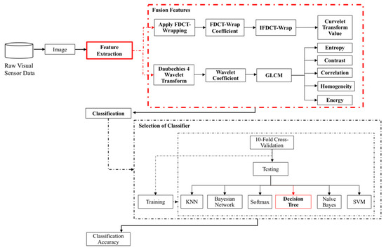
Figure 1. Process flow of the proposed CW-GLCM method for apple classification.

3.1. Feature Extraction

The phase of the proposed method feature extraction comprises of three major methods, which are Curvelet, Wavelet and GLCM method. The proposed method combines the Curvelet features with five GLCMs features extracted based on the Wavelet coefficient. To retain the image information, the image normalization step is skipped in the proposed method to deal with the low-quality region on the apple skin images. This is to avoid misclassification between defective and non-defective apple.

3.1.1. Curvelet Transform

The main reason that the proposed method fuses the Curvelet features is to detect the low-quality apple images region for curves, corners and profiles. As compared with other transform, the performance of the Curvelet transform are extremely well in capturing the edges and other singularities along the curves [71]. The Curvelet features will provide more information on low-quality regions in the apple images. In the proposed method, the Curvelet transform based on wrapping of specially selected Fourier samples (FDCT-Wrap) is used because it is the fastest and well-adapted Curvelet transform algorithm to represent edges [72,73,74]. The FDCT-Wrap is applied to enhance the image contrast of the low-quality region. The two consecutive regions between the low-quality regions that has a different pixel value with the nearby region are likely to form “edges”. This edges are formed based on the variation of pixel values allowing the FDCT-Wrap in the proposed method to detect this edges information. In order to obtain the dominant features, the LL sub-bands filter is applied to set the intensity elements of the FDCT-Wrap coefficient. Then, the inverse transformation is performed on the extracted features from the FDCT-Wrap coefficient to produce the Curvelet transform value. The steps of FDCT-wrap are as follows:

Step 1. Input the original image;

Step 2. Apply 2D Fast Fourier Transform (2DFFT) on the original image; produce a set of Fourier sample $\widehat{f}\left[n_1,n_2\right]$;

Step 3. Resample a set of Fourier sample $\widehat{f}\left[n_1,n_2\right]$ at each pair of scale $j$ and angle direction $l$ in frequency domain. The scale is from finest to coarsest scale with the angle direction start from the top-left corner increases clockwise. This will produce the new sampling function as expressed in (1).

$$\widehat{f}\left[n_1,n_2-n_1\tan {\theta }_l\right],\hspace{1em}\left(n_1,n_2\right)\in \left\{\left(n_1,n_2\right), n_{1,0}\le n_1\le n_{1,0}+L_{1,j}, n_{2,0}\le n_2<n_{2,0}+L_{2,j}\right\},$$

(1)

where $n_{1,0}$ and $n_{2,0}$ are the initial position of window function ${\tilde{u}}_{j,l}\left[n_1,n_2\right]$, $L_{1,j}$ and $L_{2,j}$ are parameter of length $2^j$ and width $2^{j/2}$ components of window function support interval. The window function formula is defined in (2).

$$\begin{gathered} {\tilde{u}}_{j,l}\left[n_1,n_2\right]=w_1\left(w_1, w_2\right)v_j\left(s_{\theta } . \frac{(2^{\left[j/2\right]}{w}_2)}{w_1}\right), \\ {w}_1\left(w_1, w_{2 }\right)= \sqrt{{\varphi }_{j+1 }^2\left(w^2\right)-{\varphi }_j^2\left(w^2\right),} \\ {\varphi }_j\left(w_1, w_{2 }\right)=\varphi \left(2^{-j}{w}_1\right)\varphi \left(2^{-j}{w}_2\right), \\ {s}_{{\theta }_1}=\left[\begin{array}{cc}1& 0\\ -\tan {\theta }_l& 1\end{array}\right], \\ \tan {\theta }_l=l\times 2^{\lfloor -j/2\rfloor }, l=-2^{\lfloor -j/2\rfloor },\dots , 2^{\lfloor -j/2\rfloor }-1 \end{gathered}$$

(2)

where $w_1$ is a vertical axis but located near the horizontal axis of $w_2$;

Step 4. The new sampling function of $\widehat{f}\left[n_1,n_2-n_1,\tan {\theta }_l\right]$ are multiplied with the window function ${\tilde{u}}_{j,l}\left[n_1,n_2\right]$:

$$\widetilde{f_{j,l}}\left[n_1,n_2\right]=\widehat{f}\left[n_1,n_2-n_1\tan {\theta }_l\right]{\tilde{u}}_{j,l}\left[n_1,n_2\right];$$

(3)

Step 5. Then, the inverse 2DFFT is applied to each of $\widetilde{f_{j,l}}$ obtained in the previous step to produce Curvelet transform value.

Finally, we extract feature vector of the Curvelet transform value and then fused them with the GLCMs features calculate based on the Wavelet transform in the following step to accomplish defective and non-defective apple classification.

3.1.2. Wavelet Transform

To improve the texture information extracted from the GLCM method, the proposed method also modifies the existing GLCM method by extracting the GLCMs features based on the Daubechies 4 Wavelet coefficient. Daubechies 4 Wavelet is chosen as it is suitable for texture classification due to their relations to multiresolution. The Wavelet coefficient will enhance the visibility of the low-quality region in the apple images, especially on the apple skin by capturing the directional edges in different resolution levels preserving the low and high frequency information. This leads the proposed method to extract better texture information from the apple images. The Wavelet transform are calculated using the wavelet function as follows:

$$W\left[\int \left(s,\tau \right)\right]=⟨\int ,{\psi }_{s,\tau }^k⟩$$

(4)

where $s\in Z$ is parameter of scale resolution level, $\tau$ is translation, $k\in \left\{h,v,d\right\}$ is the orientation and ${\psi }_{s,\tau }^k=\left(\frac{1}{\sqrt{s}}\right) {\psi }^k\left(\frac{x-\tau }{s}\right)$ is a wavelet family. The orientation $h$, $v$ and $d$ parameter represent horizontal, vertical and diagonal direction. The wavelet decomposition is achieved when the value of $s=2^j$ and $\tau =2^j.n,j,n\in Z$.

The wavelet and scaling family are constructed using wavelet function $\psi \left(x\right)$ and scaling function $\phi \left(x\right)$ as expressed in (5).

$${\psi }_{j,n}^k\left(x\right)=\frac{1}{\sqrt{2^j}} {\psi }^k\left(\frac{x-2^j.n}{2^j}\right)\mathrm{and} {\phi }_{j,n}^k\left(x\right)=\frac{1}{\sqrt{2^j}} {\phi }^k\left(\frac{x-2^j.n}{2^j}\right)$$

(5)

The two dimensional Wavelet transform are constructed based on the combination of high-pass and low-pass digital filter banks and down-samplers. As the images is in 2D signal, separable function Discrete Wavelet Transform is used in the configuration of DWT structure. The rows and columns of the images are subjected to the 1D Wavelet Transform separately to produce the 2D-DWT. The output of the decomposed images in 2D orthogonal wavelet representation resulting four orthogonal sub-bands component which are Low-Low (LL), Low-High (LH), High-Low (HL) and High-High (HH) as presented in Figure 2. The results shown in the figure is for one level decomposition. Every stage of DWT requires high-pass and low-pass digital filter with two down sampling [75]. This process is further continued and decomposed to another four sub-band components, forming two-level decomposition. The wavelet decomposition at two resolution levels as illustrates in Figure 3.

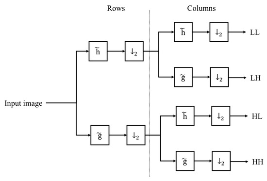
Figure 2. Image decomposition using analysis filter banks. Note that $\tilde{\mathrm{h}}$ is low-pass filter and $\tilde{\mathrm{g}}$ is high-pass filer and ↓2 is keeping one sample out of two (down sampling).

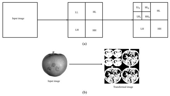
Figure 3. 2D-DWT wavelet decomposition at two resolution levels (a) the structure diagram, (b) apple image via wavelet decomposition at two resolution levels.

3.1.3. GLCM

The GLCMs texture features are extracted from GLCM based on the computed Wavelet coefficient from the prior process in Section 3.1.2. The GLCMs features are included in the proposed method to estimate the apple images texture properties. Instead of calculating the GLCMs features from GLCM coefficient, the proposed method modifies the original GLCM implementation by using Wavelet coefficient to calculate five of the GLCMs feature. The features are entropy, contrast, correlation, homogeneity and energy. The entropy is a measure of levels disorderliness and randomness in the images. It is the most dominant statistical features and widely used to measure variations between pixel intensities [71]. This is important to symbolize texture that appear in the apple images. The contrast measures the variation values and intensity contrast of the neighboring pixel in the gray level. The correlation features are also selected since it measures the correlated pixels to the neighbors over the whole image and determined the linear dependencies of the gray levels. Homogeneity features are important to measure the uniform region in the images according to its gray level difference and the energy returns the sum value of the squared elements in the GLCM. To extract the texture features from GLCM, the matrix must be symmetric [76]. In order to get a symmetric matrix, the GLCM is transposed and added to the original GLCM. From the symmetrical GLCM, the texture features are extracted. To compute the GLCM, the spatial relationship between two pixels is establish. The first one is the reference pixel which is pixel-of-interest and the other pixel is a neighbor pixel. This process forming the GLCM that contains different combination of pixel gray values. The number of gray levels $\left(G\right)$ is ranging from 0 to $G-1$. The GLCM is highly dependent on two parameters which are distance between the pixel pair ($D)$ and their angular relationship ($\theta )$. In the proposed method, the GLCM is computed based on the predefine distance of one pixel ($D=1)$ and $\theta$ are quantized in four parameter directions which are $0^{°},{45}^{°},{90}^{°}$ and ${135}^{°}.$ The directionality of GLCM used in the proposed method illustrated as in Figure 4. This forms four co-occurrences matrix. The GLCM are calculated in the corresponding matrix by taking the absolute value of each resolution level of the Wavelet coefficient matrix obtained using 2D-DWT in the prior section. Then, each of the GLCMs texture features are computed from the details of the Wavelet coefficient matrix for various resolution level in the corresponding matrix.

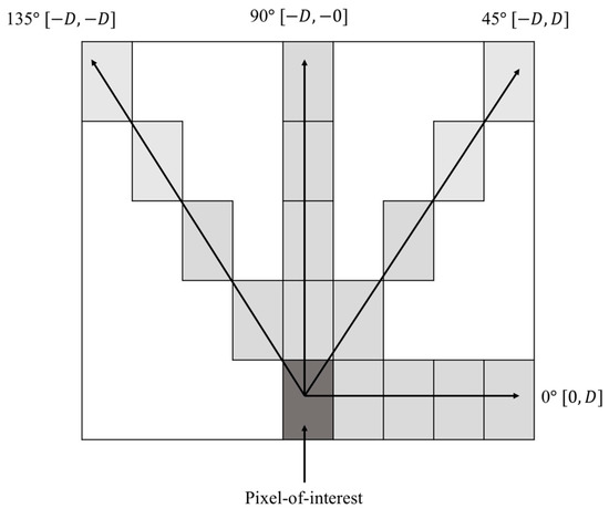
Figure 4. Directionality of GLCM.

The procedure of the extraction of GLCMs features based on the Wavelet Coefficient are as follows:

Step 1. Input the original image;

Step 2. Compute GLCM from the wavelet coefficient and calculate based on five GLCMs. The formulations for each of the GLCMs features are computed as follows:

$$\mathrm{Entropy}={{\displaystyle \sum }}_{i=0}^{G-1}{{\displaystyle \sum }}_{j=0}^{G-1}P\left(i,j\right)\ast \log \left(P\left(i,j\right)\right),$$

(6)

$$\mathrm{Contrast}={{\displaystyle \sum }}_{i=0}^{G-1}{n}^2\{{\displaystyle \sum }_{i=1}^G{\displaystyle \sum }_{j=1}^{G}P\left(i,j\right)\},\left|i-j\right|=n,$$

(7)

$$\mathrm{Correlation}={\displaystyle \sum }_{i=0}^{G-1}{\displaystyle \sum }_{j=0}^{G-1}\frac{\{i\ast j\}\ast P\left(i,j\right)-\{{\mu }_x\ast {\mu }_y\}}{{\sigma }_x\ast {\sigma }_y},$$

(8)

$$\mathrm{Homogeneity}={\displaystyle \sum }_{i=0}^{G-1}{\displaystyle \sum }_{j=0}^{G-1}\{\frac{P\left(i,j\right)}{1+\left|i-j\right|}\},$$

(9)

$$\mathrm{Energy}={\displaystyle \sum }_{i=0}^{G-1}{\displaystyle \sum }_{j=0}^{G-1}P{\left(i,j\right)}^2,$$

(10)

where $P$ is a pixel, $i$ is row $j$ is column,$n$ is line of neighborhood, $G$ represents the number of gray levels used, ${\mu }_x,{\mu }_y$, ${\sigma }_x,{\sigma }_y$ are the mean and standard deviation value obtained from $P_x$ and $P_y$ respectively. The $P_x$ and $P_y$ are the results obtained after summing the rows $P\left(i,j\right)$;

Step 3. Acquire texture features according to (6), (7), (8), (9) and (10).

Finally, the Curvelet features obtained from the prior process in Section 3.1.1 are fused in the texture features obtained in step 3 to produce highly informative fusion features. The parameter settings of Curvelet, Wavelet and GLCM used in the proposed method are summarized in Table 1.

Table 1. Parameters setting of Curvelet, Wavelet and GLCM.

Algorithm	Parameters	Settings
Curvelet	scale $\left(j\right)$	3
	number of angles at the second coarsest level ($l)$	16
	fine	2
Wavelet	level of decomposition $\left(s\right)$	2
	number of minimum scale	7
	number of vanishing moments	4
	gray levels $\left(G\right)$	$0 \mathrm{to}G-1$
	total number of directions	3
GLCM	angle ($\theta$)	$0^{°},{45}^{°},{90}^{°}$ and ${135}^{°}$
	$\mathrm{distance}\mathrm{pixel}\left(D\right)$	1
	texture features	entropy, contrast, correlation, homogeneity and energy

3.2. Classification

In the classification phase, the fusion features extracted in the previous phase are classified into the defective and non-defective apples. One of the major challenges in classifying large number of features is to determine the suitable classifier that able to achieve better classification accuracy [77]. Therefore, to ensure the optimal performance for the proposed features, six classifiers which are K-Nearest Neighbors (KNN), Bayesian Network, Softmax, Decision Tree, Naïve Bayes and Support Vector Machine (SVM) are tested. These classifiers are selected based on each of their specific advantage. The KNN classifier is among the most widely used classifier for image classification task. This is because of its simplicity and easy to be implemented [78]. In contrast, the Bayesian Network are the classifier that based on their bias-variance trade-off network structure. The network structure models will allow the Bayesian Network to precisely capture the fine details in the data [79]. Another simple and fast classifier that can achieve accurate result in most cases are the Decision Tree Classifier [80]. Furthermore, it also works well with the noisy data [80]. The Naïve Bayes are also an efficient and effective machine learning classifier [81,82,83], while Softmax classifier is one of the most commonly-used logistic regressions classifier especially for multi-class classification [84,85]. Finally, the SVM classifier are also selected due to it is well established technique in many image recognition tasks and its high accuracy performance [78,86,87,88,89]. Their performance is evaluated and a test decision of the best performing classifier on the proposed method determine the suitable classifier for the proposed method.

4. Experiments

To demonstrate the reliability of the proposed CW-GLCM method, a series of comprehensive experiments is conducted in VLSI laboratory Faculty of Computer Science and Information Technology, University of Malaya, Kuala Lumpur, Malaysia. All the experiments are conducted using MATLAB R2017b (MathWorks, Natick, MA, USA) on a computer with the following specification: Windows 10 Pro and an Intel Core i7-4770 CPU (3.4GHz) processor with 8.00 GB RAM. The details of the experiments and evaluation are described in the subsections below.

4.1. Datasets

Instead of analyzing the performance only against defective and non-defective, we also evaluated the method on low-quality region as well. Due to the shortage of defective and non-defective images datasets that comprises low-quality region, two newly apple image datasets are created, namely NDDA and NDDAW datasets. The NDDA generally consist of various types of apple images, while the NDDAW consist of more apple images with low-quality region on its skin. Each of the dataset are classified into two categories of non-defective and defective. The non-defective and defective classification are verified by the agriculture practitioners from Malaysian Agricultural Research and Development Institute (MARDI) and Pahang Agriculture Department. The datasets are collected using vision sensors and some of the apple images were collected via the Google search engine with several keywords such as “fresh + apple”, “healthy + apple”, “apple + disease”, “damage + apple”, “defect + apple” and “low + grade + apple + fruit”. This is due to the difficulties in obtaining various types of defective apple. Most of the apple images obtained from Google search engine are center, clean and occupied most of the image without or very few cluttered environments. This is similar to the data acquisition via vision sensor in the research that captures apple images placed on the conveyor belt as illustrated in Figure 5. To ensure the quality of the images, the light sources are placed near to the vision sensor and are uniformly distributed. This is done to reduce the effect of shadows and glare. The image resolution of all the images captured using vision sensor are 900 × 700 pixel. While the resolution of the images obtained via Google search engine may vary from 205 × 220 pixel to 552 × 512 pixel. Each of the images obtained from Google search engine in both datasets are rescaled to 900 × 700 pixel following the resolution setting of the images captured via vision sensor. Datasets are available online at https://github.com/AsIsmail/Apple-Dataset. The details of each dataset are described in the following subsections.

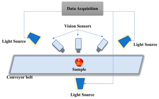
Figure 5. Illustration of the data acquisition process using vision sensors.

4.1.1. NDDA

This dataset consists of 550 apple images; in which 275 of the images are the non-defective apples and 275 are the defective apples. For both categories in the dataset, the natural parts of the apple are also included which are the stem end (370 images) and calyx (61 images). In this dataset, apples with low-quality region on its skin are 76 images. The properties of this dataset are shown in Table 2. The non-defective apple images were collected from five apple cultivars which are Red Delicious, Gala, Fuji, Honeycrisp and Granny Smith. While the defective category was collected from five groups of defects which is Scab, Rot, Cork Spot, Blotch and Bruise. The defective category includes variations severity of external defects, which is visible to the naked eyes with different location, region and size. A sample images of the dataset is shown in Figure 6.

Table 2. Details of the characteristics in NDDA dataset.

Non-Defective		Defective
Cultivars	Total	Types	Total
Red Delicious	53	Scab	71
Gala	57	Rot	79
Fuji	58	Cork Spot	61
Honeycrisp	56	Blotch	32
Granny Smith	51	Bruise	32
Total	275	Total	275

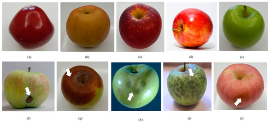
Figure 6. Examples of apple images in the NDDA dataset. The first row is the examples of non-defective apples and the second row is the example of defective apples: (a) Red Delicious, (b) Gala, (c) Fuji, (d) Honeycrisp, (e) Granny Smith, (f) Scab, (g) Rot, (h) Cork Spot, (i) Blotch, (j) Bruise.

4.1.2. NDDAW

On the other hand, the NDDAW dataset consists of 560 apple images classified into two categories of non-defective and defective. The NDDAW dataset is composed of 280 non-defective apples and 280 defective apples. The overall setup of this dataset follows the NDDA dataset. However, the NDDAW dataset are more complex compared to NDDA as it consists more apple images with low-quality region on its skin (159 images), which intended to address the limitation of classifying low-quality image region. In the dataset, a total of 248 apple images with stem end and 130 apple images with calyx are also included. The properties and sample of NDDAW dataset are shown in Table 3 and Figure 7.

Table 3. Details of the characteristics in NDDAW apple dataset.

Non-Defective		Defective
Cultivars	Total	Types	Total
Red Delicious	44	Scab	42
Gala	16	Rot	55
Fuji	26	Cork Spot	27
Honeycrisp	59	Blotch	7
Granny Smith	135	Bruise	149
Total	280	Total	280

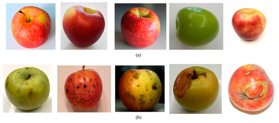
Figure 7. Examples of images in the NDDAW dataset. (a) Non-defective; (b) defective.

4.2. Evaluation Metrics

In this research, K-fold cross-validation is used to evaluate the performance of the proposed CW-GLCM method. The value of K strongly depend on the overall quantity of the data and the suggested number of fold is between 5 to 10 fold [90,91]. Based on our prior work in [1], K parameter of 10 yields the highest classification accuracy. Thus, the 10-fold cross-validation is used in this experiment. The aforementioned performance evaluation technique is also considered in this research since most of the work related to this domain from the literature use the 10-fold cross-validation to evaluate performance measure in their work [30,90,92,93]. The classification performance is measured in terms of precision, recall and accuracy. For 10-fold cross-validation, the dataset will be randomly partitioned into ten number of folders in which every fold will have virtually the same number of class distribution. One of the folders will be used for validation while the remaining nine folders will be used for training. This process is repeated ten times until each of the folders is used exactly once as a validation set. Finally, the average results from the ten experiments are calculated. The classification is defined as follows:

$$\mathrm{Precision}=\mathrm{TP}/\left(\mathrm{TP}+\mathrm{FP}\right),$$

(11)

$$\mathrm{Recall}=\mathrm{TP}/\left(\mathrm{TP}+\mathrm{FN}\right),$$

(12)

$$\mathrm{Accuracy}=\left(\mathrm{TN}+\mathrm{TP}\right)/\left(\mathrm{TP}+\mathrm{FN}+\mathrm{FP}+\mathrm{TN}\right),$$

(13)

where TP, FP, TN and FN are defined in Table 4.

Table 4. Terminology and derivations of the evaluation metrics.

Terminology	Derivations
TP (true positive)	Defective apple is correctly classified as defective apple.
TN (true negative)	Non-defective apple correctly classified as non-defective apple.
FP (false positive)	Defective apple incorrectly classified as non-defective apple.
FN (false negative)	Non-defective apple is incorrectly classified as defective apple.

In each of the experiments, the computational time is also recorded.

4.3. Performance Measure for Fusion Features

As highlighted in Section 3, the fusion features are the combination of Curvelet features and five GLCMs features based on the Wavelet coefficient. This forming a set of fusion features which consist of six features. They are the Curvelet features, entropy, contrast, correlation, homogeneity and energy. In searching for the best fusion features, the fusion features are compared with the Curvelet features and each of the GLCMs features calculated from GLCM coefficient. Their performances are evaluated and compared with our proposed fusion features on NDDA dataset using SVM classifier as shown in Table 5. Based on the table, the results show that our proposed fusion features outperformed others with 88.89% precision, 85.71% recall and 87.04% accuracy. Although the fusion features require the longest time for training and testing, the results proved that the Curvelet and Wavelet transform can improve the detection of the GLCM texture features.

Table 5. Comparative results (precision, recall, accuracy, training time and testing time) for the proposed fusion features using SVM classifier on NDDA.

Features	Precision (%)	Recall (%)	Accuracy (%)	Training Time (s)	Testing Time (s)
Curvelet	77.78	75.00	75.93	317.34	2.97
Contrast	58.57	54.67	55.00	103.29	1.51
Correlation	53.57	52.26	52.32	107.91	0.72
Energy	67.14	58.02	59.29	101.09	0.32
Homogeneity	56.07	55.28	55.36	100.73	0.37
Entropy	78.21	57.94	60.71	101.35	0.32
Fusion features (proposed features)	88.89	85.71	87.04	364.51	3.12

A graphical comparison performance between the proposed fusion features with contrast, correlation, energy, homogeneity, entropy and Curvelet using SVM classifier on NDDA dataset are presented in Figure 8. Based on the Figure 8a, the proposed fusion features is shown to be able to obtain the highest percentage for all measurement of precision, recall and accuracy compared to other features with a minimum value of 85.71% on recall. However, it requires the longest time for the training and testing as shown in Figure 8b. This is due to the reason that the fusion features incorporate three major methods which is the Curvelet, Wavelet and the GLCM method. In addition, the normalization step is skipped in the feature extraction phase to retain the information of a low-quality region on the apple skin images. This will increase the time complexity and reduce the speed. Although the fusion features show high computational time, from these results it can be seen that the fusion features of Curvelet features with five GLCMs features calculated based on the Wavelet coefficient outperformed others in term of the precision, recall and accuracy.

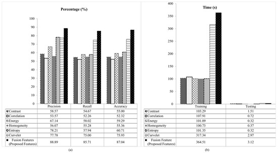
Figure 8. Comparative results of the proposed fusion features using SVM classifier on NDDA dataset (a) precision, recall and accuracy, (b) training and testing time.

To obtain the most suitable classifier, the fusion features utilize six classifiers and are tested on NDDA dataset. The selections of classifiers are KNN, Bayesian Network, Softmax, Decision Tree, Naïve Bayes and SVM. The results for each classifier are presented in Table 6.

Table 6. Comparison of the proposed fusion features with different classifiers on NDDA dataset.

Classifier	Fusion Features (Proposed Features)
	Precision (%)	Recall (%)	Accuracy (%)	Training Time (s)	Testing Time (s)
KNN	70.37	73.08	72.73	386.19	23.55
Bayesian Network	70.37	76.00	74.07	385.97	0.57
Softmax	79.31	71.88	73.21	372.24	1.10
Decision Tree	96.30	100.00	98.15	344.17	0.25
Naïve Bayes	59.26	76.19	70.37	390.18	0.98
SVM	88.89	85.71	87.04	364.51	3.12

From the Table 6, the fusion features with Decision Tree classifier give the best performance for all for the measurement of precision, recall and accuracy including the computational time. The comparative results for different classifier are presented in Figure 9.

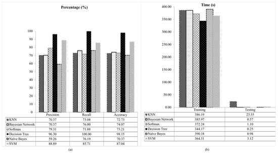
Figure 9. Comparative results of fusion feature for different classifier on NDDA dataset (a) precision, recall and accuracy, (b) training and testing time.

Based on Figure 9, the Decision Tree classifier outperformed others with 96.30% of precision, recall 100% and accuracy 98.15%. In contrast, Naïve Bayes classifier shows the lowest performance for precision (59.26%) and accuracy (70.37%). This is because Naïve Bayes classifier make a very strong assumption that all variables are mutually correlated and contribute towards classification. Due to this assumption, it degrades the classification performance [80]. The lowest recall is observed in Softmax classifier with 71.88%. The performance decrease in term of recall rate in the Softmax classifier is due to overfitting from high-variance structure [84]. In terms of computational time among the classifiers, Naïve Bayes takes the longest time for training (390.18 s), whereas KNN for testing (23.55 s). The Naïve Bayes classifier is based on probabilistic that requires the knowledge of prior probability distribution of the class and also data to be classified. This increased the training time in Naïve Bayes classifier. Conversely, the KNN classifier is computationally intensive as it stores all the training data and compares the extracted features on the test images with each training data for classification [78]. In contrast, the Decision Tree classifier is the fastest classifier during the training (344.17 s) and testing (0.25 s). The results also show that the Decision Tree classifier able to achieve the highest performance for all measurements. This is due to the reason that different ranges of features in our fusion features does not affect the Decision Tree. While in the SVM and other classifiers, each of the data instances is represented in the form of real numbers vectors [1]. This transformation may affect the classification performance. Since the data normalization step is skipped in our feature extraction stage, the Decision Tree classifier is found to be more suitable to classify our fusion features. Therefore, in the proposed method, the Decision Tree classifier is chosen.

4.4. Comparison with Existing Methods

To further evaluate the performance of the proposed method, five existing methods for image recognition are compared with the proposed method. They are BOW [15], SPM [16], CNN [17], Texture analysis [18] and CLAHE + GLCM + ELM [19]. The average results for 10-fold cross-validation of each method are presented in Table 7.

Table 7. Comparison of confusion matrix for BOW [15], SPM [16], CNN [17], Texture analysis [18], CLAHE + GLCM + ELM [19] and the proposed CW-GLCM method on NDDA dataset: Defective (D) and Non-defective (N).

Class	Methods
	BOW		SPM		CNN		Texture Analysis		CLAHE + GLCM + ELM		CW-GLCM (Proposed Method)
	D	N	D	N	D	N	D	N	D	N	D	N
D	24	3	26	1	25	2	20	7	22	5	26	1
N	4	23	0	27	1	26	4	23	11	16	0	27
Precision (%)	88.89		96.30		92.59		74.07		81.48		96.30
Recall (%)	85.71		100		96.15		83.33		66.67		100
Accuracy (%)	87.04		98.15		94.44		79.63		70.37		98.15
Training time (s)	402.94		150.97		149.13		135.12		1323.58		344.17
Testing Time (s)	3.92		0.13		0.08		1.38		0.02		0.25

Following the 10-fold cross-validation experiment on NDDA dataset, a total number of 275 images from the defective class and 275 images from the non-defective class are divided into ten equal parts. Each part consists of 28 or 27 images of the defective and non-defective classes. Nine parts are used for training and one for testing. This process is repeated ten times until each of the folders is used exactly once as a validation set. Then, the average value for all ten experiment are taken. In Table 7, the classification performance is led by the proposed CW-GLCM and SPM method with 98.15% classification accuracy. Both methods correctly classified all 27 images of non-defective apples followed by CNN (26 images), BOW and Texture analysis (23 images), while the lowest goes to CLAHE + GLCM + ELM (16 images). For the defective images, the proposed CW-GLCM and SPM method correctly classified 26 out of 27 images of defective apples while CNN, BOW, CLAHE + GLCM + ELM and Texture analysis correctly classified 25, 24, 22 and 20 respectively.

Overall, our proposed CW-GLCM and SPM method outperformed others in NDDA dataset with the classification accuracy of 98.15%. This is followed by CNN with 94.44%, BOW 87.04%, Texture analysis 79.63% and CLAHE + GLCM + ELM 70.37% as presented in Table 7. The proposed CW-GLCM and SPM method also outperformed others with 96.30% precision and 100% recall rate. Among the methods, CLAHE + GLCM + ELM take the longest time for training (1323.58 s) and the fastest during testing (0.02 s). The CLAHE + GLCM + ELM method required the longest time for training due to the computationally extensive of CLAHE approach in the method. The CLAHE approach are usually used for image enhancement in off-line application [63]. In contrast to the training time, the CLAHE + GLCM + ELM able to classify the dataset faster compared to other methods because of the extremely fast learning speed of the Extreme Learning Machine (ELM) classifier used in the method [19]. This is followed by the CNN method with 0.08 s, SPM 0.13 s, proposed CW-GLCM 0.25 s, texture analysis 1.38 s and BOW 3.92 s. The BOW requires the longest time for testing the NDDA dataset because of the high computational cost in vector quantization step in BOW method [1]. In contrast to BOW, the CNN method able to classify faster because of the input images to the CNN method were rescaled from the original of 900 × 700 pixels to 227 × 227 pixels. This is due to the CNN requirement of having fixed-size input images [7,8]. If the arbitrary sizes of the images are applied, the CNN method will fit the images input to its fixed size via either cropping or warping the images [7,8,94,95]. Although our proposed CW-GLCM requires a longer time to classify the dataset than the SPM method, the results are still acceptable as it takes only less than 0.23 s longer than the CLAHE + GLCM + ELM, which is the fastest method during testing to successfully classify all the non-defective apple images. Other than that, the proposed CW-GLCM only misclassified one out of 27 defective apples. These results indicate that our proposed method able to effectively classify between defective and non-defective apple including the apple with a low-quality region on its skin. The examples of the low-quality region on the non-defective apple images can be found in bright-skinned apple and apple with yellow-white flecks as shown in Figure 10. In other methods, these types of apple may be misclassified as defective.

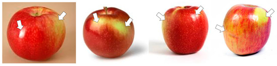
Figure 10. Examples of misclassified apple images with a low-quality region. The low-quality regions on apple skin images are pointed by the arrows.

4.5. Analysis of Classification Accuracy Against Low-Quality Region

Based on the analysis of the proposed method on the NDDA dataset, the results were further explored. The proposed method is tested with NDDAW dataset in which the dataset was created particularly to include more low-quality apple image region. This dataset consists of 159 apple images with a low-quality region on its skin. The comparison average results for 10-fold cross-validation with other methods are presented in Table 8.

Table 8. Confusion matrix for BOW [15], SPM [16], CNN [17], Texture analysis [18], CLAHE + GLCM + ELM [19] and proposed CW-GLCM method on NDDAW dataset: Defective (D) and Non-defective (N).

Class	Methods
	BOW		SPM		CNN		Texture Analysis		CLAHE + GLCM + ELM		CW-GLCM (Proposed Method)
	D	N	D	N	D	N	D	N	D	N	D	N
D	21	7	20	8	22	6	20	8	14	14	24	4
N	5	23	9	19	6	22	13	15	11	17	2	26
Precision (%)	75.00		71.43		78.57		71.43		50.00		86.79
Recall (%)	80.65		68.97		78.57		60.61		56.00		91.01
Accuracy (%)	78.50		69.64		78.57		62.50		53.36		89.11
Training time (s)	275.61		149.92		146.89		131.32		2075.93		386.63
Testing Time (s)	3.84		0.47		0.34		1.41		0.02		0.31

Following the 10-fold cross-validation for NDDAW dataset, a total number of 280 images from the defective class and 280 images from the non-defective class are divided into ten equal parts. Each part consists of 28 images of the defective and non-defective classes. Nine parts are used for training and one for testing. This process is repeated ten times until each of the folders is used exactly once as a validation set. Then, the average value for all ten experiment are taken. From Table 8, the classification performance is led by the proposed CW-GLCM method with 89.11% classification accuracy. This is followed by CNN 78.57%, BOW 78.50%, SPM 69.64%, Texture analysis 62.50% and CLAHE + GLCM + ELM 53.36%. The proposed CW-GLCM correctly classified 26 images out of 28 non-defective apples while CNN (22 images), BOW (23 images), SPM (19 images), Texture analysis (16 images) and CLAHE + GLCM + ELM (17 images). For the defective images, the proposed CW-GLCM method correctly classified 24 images of defective apples followed by CNN (22 images), BOW (21 images), SPM and Texture analysis (20 images) while CLAHE + GLCM + ELM (14 images). In this dataset, the proposed CW-GLCM outperformed others whereas the CLAHE + GLCM + ELM method recorded the lowest classification accuracy followed by Texture analysis method.

Overall, the CLAHE + GLCM + ELM method recorded the lowest classification accuracy performance in both datasets tested. This is due to the drawbacks of the CLAHE approach that sometimes may produce unwanted gray level artifact and creates an equal density in all the histogram bins during the image enhancement process [62]. In contrast, the obvious accuracy performance difference can be observed from the SPM method between NDDA and NDDAW dataset. Although the SPM method achieved high percentage for the measurement of precision, recall and accuracy in NDDA dataset, it presents lower performance in NDDAW dataset. This is because the NDDAW dataset contains more apple images with low-quality region compared to NDDA dataset. The result shows that the SPM method is less sensitive in detecting features in the low-quality region. On the other hand, our proposed CW-GLCM method achieved the highest classification accuracy, precision and recall in both datasets. This indicates that the proposed method is more robust in detecting features on low-quality region. Figure 11a,b depicts the performance of precision, recall and accuracy for NDDA and NDDAW. The training and testing time tested on each dataset are presented in Figure 11c,d.

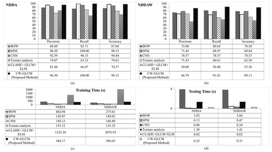
Figure 11. Comparative results of precision recall and accuracy in (a) NDDA dataset, (b) NDDAW dataset, (c) training time and (d) testing time for BOW [15], SPM [16], CNN [17], Texture analysis [18], CLAHE + GLCM + ELM [19] and proposed CW-GLCM method.

4.6. Performance Evaluation with Different Image Resolution

To evaluate the efficiency of the proposed method against different image resolution, the test with three different image resolution (i.e., original, small and large) is conducted. The small and large images are created by rescaling them with two parameters, 0.5 and 1.5. The comparative results of their precision, recall, accuracy, training and testing time are presented in Table 9.

Table 9. Comparative results (precision, recall, accuracy, training time and testing time) of the proposed method for different resolution images.

Rescale	Resolution (Pixel)	Precision (%)	Recall (%)	Accuracy (%)	Training Time (s)	Testing Time (s)
0.5	450 × 350	96.30	1.00	98.15	102.76	0.12
Original	900 × 700	96.30	1.00	98.15	344.15	0.25
1.5	1350 × 1050	96.30	1.00	98.15	550.74	0.31

From the results, it can be seen that the performance of the proposed CW-GLCM is not affected by the resolution change. The only difference observed is in the computational time. The time taken for training and testing is getting higher as the number of resolutions increased. The results proved that the image resolution does not influence the precision, recall and accuracy of the proposed CW-GLCM. Although the training and testing time are increased with the increment of image resolution, the 10-fold cross-validation experiment on the dataset shows that the proposed method are able to process 27 images within 0.25 s during testing on the original resolution (900 × 700 pixel). These results indicate that the proposed CW-GLCM method can be used in real-time systems.

5. Discussion

Overall, the proposed CW-GLCM method outperformed others in detecting important features on the low-quality apple image region. The proposed method performance exceeds 86.79% for all the performance measures in both datasets tested. In contrast, a lower precision, recall and accuracy are observed in the other five methods on NDDAW dataset with the maximum recall of 80.65% in BOW method. The classification accuracy of BOW in NDDAW dataset is 78.50%, SPM 69.64%, CNN 78.57%, Texture analysis 62.50% and CLAHE + GLCM + ELM 53.36%. The lower classification accuracy of the BOW, SPM, Texture analysis and CLAHE + GLCM + ELM methods is influenced by the presence of low-quality region on the apple images in NDDAW dataset. While the reasons that reduce the classification accuracy of the CNN method is due to the small sample dataset utilized in the experiment. The CNN deep learning method requires a large number of images for training in order to obtain a desired classification accuracy result [1,7,8,9,10]. In contrast, the proposed CW-GLCM are able to achieve more than 86.79% for precision, 91.01% recall and 89.11% accuracy for both datasets tested. This indicates that the introduction of Curvelet features and Wavelet Coefficient in the GLCM method can improve the results even with low quality region images in small sample dataset. This is possible since the Curvelet and Wavelet transform able to enhance the apple images, especially on the low-quality region. However, the detection failure can still be observed on the defective apple that had been misclassified as non-defective apple. The example of the false positive classification in which defective apple incorrectly classified as non-defective apple is shown in Figure 12. This blemish defect region may be misclassified as stem ends or calyxes which are the natural parts of the apple that located at the top and bottom of the apple. This is due to similarities exist between these features.

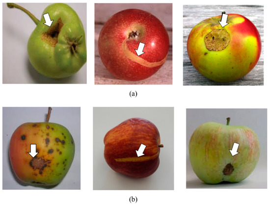
Figure 12. Examples of the detection failures of the proposed CW-GLCM on (a) NDDA and (b) NDDAW. The defect region is pointed by the arrows.

6. Conclusions

The CW-GLCM method is proposed for apple classification to differentiate between defective and non-defective apple. The proposed methods fused the Curvelet and Wavelet transform with the GLCM method to improve its ability in detecting features on the low-quality region of apple images. In apple classification, it is crucial to detect these features to enable the classifier to differentiate and correctly classify between defective and non-defective apple. Comparative experiments have been performed between the proposed CW-GLCM method with other five existing methods namely BOW [15], SPM [16], CNN [17], Texture analysis [18] and CLAHE + GLCM + ELM [19]. Experimental results show that the proposed CW-GLCM and SPM method attained higher classification accuracy in NDDA dataset with the same precision (96.30%), recall (100%) and accuracy (98.15%). However, lower classification accuracy is observed in SPM method when tested with NDDAW dataset with 71.43% precision, 68.97% recall and 69.64% accuracy. In contrast, our proposed CW-GLCM able to achieve 86.79% precision, 91.01% recall and 89.11% accuracy. In comparison with other methods, our proposed method presents the highest precision, recall and accuracy results in both datasets tested. The result shows that the proposed CW-GLCM method are more robust and can effectively classify between defective and non-defective apple including the apple images with low-quality region.

7. Future Works

This paper proposed a new method of fusion features namely CW-GLCM for apple classification in smart manufacturing with a goal to optimize productivity. The optimization can be performed using the data analytics and visualization that requires accurate and reliable informative data as the input for analytics model. The result shows that the proposed CW-GLCM method able to effectively classify the defective and non-defective apple including low-quality apple image region. Therefore, it can be used in assisting the decision-making in apple manufacturing industry. Though the proposed CW-GLCM method is superior to other existing methods and achieves more accurate classification in both datasets tested, the method was shown to be less effective in detecting some of the defective apples as shown in Section 5. In the future, we will concentrate on improving these drawbacks and also will consider on increasing the diversity of apple images dataset using the data augmentation techniques for more advanced deep learning method. However, the key challenge for the data augmentation is it is very computationally expensive to generate enough samples for training on a large neural network. Furthermore, due to particularities of various types of the defect, severity and cultivar of apple images in this research, it will become a major challenge for the data augmentation. The overly augmented and redundant augmentation may also introduce biases into the dataset and can slow down the training [96,97]. These will become the focus area for our future work and extend its implementation for multi-class classification. We intend to perform multi-class classification to classify different types of defective apples for further data analytics. Based on the current production data of the defective types in apple production, the data analytics process will identify the patterns and learns for future planning and prediction to improve the apple growth.

References

- Ismail, A.; Idris, M.Y.I.; Ayub, M.N.; Por, L.Y. Vision-Based Apple Classification for Smart Manufacturing. Sensors 2018, 18, 4353. [Google Scholar] [CrossRef] [PubMed]
- Moyne, J.; Iskandar, J. Big data analytics for smart manufacturing: Case studies in semiconductor manufacturing. Processes 2017, 5, 39. [Google Scholar] [CrossRef]
- Nagorny, K.; Lima-Monteiro, P.; Barata, J.; Colombo, A.W. Big data analysis in smart manufacturing: A review. Int. J. Commun. Netw. Syst. Sci. 2017, 10, 31–58. [Google Scholar] [CrossRef]
- Raghupathi, W.; Raghupathi, V. Big data analytics in healthcare: Promise and potential. Health Inf. Sci. Syst. 2014, 2, 3. [Google Scholar] [CrossRef] [PubMed]
- Wan, J.; Tang, S.; Li, D.; Wang, S.; Liu, C.; Abbas, H.; Vasilakos, A.V. A manufacturing big data solution for active preventive maintenance. IEEE Trans. Ind. Inform. 2017, 13, 2039–2047. [Google Scholar] [CrossRef]
- Shin, S.-J.; Woo, J.; Rachuri, S. Predictive analytics model for power consumption in manufacturing. Procedia Cirp 2014, 15, 153–158. [Google Scholar] [CrossRef]
- Krizhevsky, A.; Sutskever, I.; Hinton, G.E. Imagenet classification with deep convolutional neural networks. In Proceedings of the Advances in Neural Information Processing Systems, Lake Tahoe, NV, USA, 3–6 December 2012; pp. 1097–1105. [Google Scholar]
- He, K.; Zhang, X.; Ren, S.; Sun, J. Spatial pyramid pooling in deep convolutional networks for visual recognition. IEEE Trans. Pattern Anal. Mach. Intell. 2015, 37, 1904–1916. [Google Scholar] [CrossRef] [PubMed]
- Xiao, Z.; Zhang, X.; Geng, L.; Zhang, F.; Wu, J.; Liu, Y. Research on the Method of Color Fundus Image Optic Cup Segmentation Based on Deep Learning. Symmetry 2019, 11, 933. [Google Scholar] [CrossRef]
- Cheng, X.; Zhang, Y.; Chen, Y.; Wu, Y.; Yue, Y. Pest identification via deep residual learning in complex background. Comput. Electron. Agric. 2017, 141, 351–356. [Google Scholar] [CrossRef]
- Deng, J.; Dong, W.; Socher, R.; Li, L.-J.; Li, K.; Fei-Fei, L. Imagenet: A large-scale hierarchical image database. In Proceedings of the 2009 IEEE Conference on Computer Vision and Pattern Recognition, Miami, FL, USA, 20–25 June 2009; pp. 248–255. [Google Scholar]
- Navarro, P.J.; Pérez, F.; Weiss, J.; Egea-Cortines, M. Machine learning and computer vision system for phenotype data acquisition and analysis in plants. Sensors 2016, 16, 641. [Google Scholar] [CrossRef]
- Service, U.F.A. Global Agricultural Information Network Report (CH17058); USDA Foreign Agricultural Service: Washington, WA, USA, 2017; p. 15. [Google Scholar]
- Li, Y.; Wang, S.; Tian, Q.; Ding, X. Feature representation for statistical-learning-based object detection: A review. Pattern Recogn 2015, 48, 3542–3559. [Google Scholar] [CrossRef]
- Csurka, G.; Dance, C.; Fan, L.; Willamowski, J.; Bray, C. Visual categorization with bags of keypoints. In Proceedings of the Workshop on Statistical Learning in Computer Vision, ECCV, Prague, Czech Republic, 11–14 May 2004; pp. 1–2. [Google Scholar]
- Lazebnik, S.; Schmid, C.; Ponce, J. Beyond bags of features: Spatial pyramid matching for recognizing natural scene categories. In Proceedings of the 2006 IEEE Computer Society Conference on Computer Vision and Pattern Recognition, New York, NY, USA, 17–22 June 2006; pp. 2169–2178. [Google Scholar]
- dos Santos Ferreira, A.; Freitas, D.M.; da Silva, G.G.; Pistori, H.; Folhes, M.T. Weed detection in soybean crops using ConvNets. Comput. Electron. Agric. 2017, 143, 314–324. [Google Scholar] [CrossRef]
- Olaniyi, E.O.; Adekunle, A.A.; Odekuoye, T.; Khashman, A. Automatic system for grading banana using GLCM texture feature extraction and neural network arbitrations. J. Food Process Eng. 2017, 40. [Google Scholar] [CrossRef]
- Li, W.; Chen, Y.; Sun, W.; Brown, M.; Zhang, X.; Wang, S.; Miao, L. A gingivitis identification method based on contrast-limited adaptive histogram equalization, gray-level co-occurrence matrix, and extreme learning machine. Int. J. Imag. Syst. Tech. 2019, 29, 77–82. [Google Scholar] [CrossRef]
- Chen, X.; Kopsaftopoulos, F.; Wu, Q.; Ren, H.; Chang, F.-K. A Self-Adaptive 1D Convolutional Neural Network for Flight-State Identification. Sensors 2019, 19, 275. [Google Scholar] [CrossRef] [PubMed]
- Toshev, A. Shape Representations for Object Recognition. Ph.D. Thesis, University of Pennsylvania, Pennsylvania, PA, USA, 2011. [Google Scholar]
- Tian, D. A review on image feature extraction and representation techniques. Int. J. Multimed. Ubiquitous Eng. 2013, 8, 385–396. [Google Scholar]
- Ojala, T.; Pietikäinen, M.; Harwood, D. A comparative study of texture measures with classification based on featured distributions. Pattern Recogn 1996, 29, 51–59. [Google Scholar] [CrossRef]
- Al-Hammadi, M.H.; Muhammad, G.; Hussain, M.; Bebis, G. Curvelet transform and local texture based image forgery detection. In Proceedings of the International Symposium on Visual Computing, Crete, Greece, 29–31 July 2013; pp. 503–512. [Google Scholar]
- Silva, C.; Bouwmans, T.; Frélicot, C. An extended center-symmetric local binary pattern for background modeling and subtraction in videos. In Proceedings of the 10th International Conference on Computer Vision Theory and Applications-Volume 1: VISAPP, Berlin, Germany, 11–14 March 2015; pp. 395–402. [Google Scholar]
- Papakostas, G.A.; Koulouriotis, D.E.; Karakasis, E.G.; Tourassis, V.D. Moment-based local binary patterns: A novel descriptor for invariant pattern recognition applications. Neurocomputing 2013, 99, 358–371. [Google Scholar] [CrossRef]
- Abdulrahman, M.; Gwadabe, T.R.; Abdu, F.J.; Eleyan, A. Gabor wavelet transform based facial expression recognition using PCA and LBP. In Proceedings of the 2014 22nd Signal Processing and Communications Applications Conference (SIU), Trabzon, Turkey, 23–25 April 2014; pp. 2265–2268. [Google Scholar]
- Ojala, T.; Pietikäinen, M.; Mäenpää, T. Multiresolution gray-scale and rotation invariant texture classification with local binary patterns. IEEE Trans. Pattern Anal. Mach. Intell. 2002, 24, 971–987. [Google Scholar] [CrossRef]
- Pietikäinen, M.; Ojala, T.; Xu, Z. Rotation-invariant texture classification using feature distributions. Pattern Recognit. 2000, 33, 43–52. [Google Scholar] [CrossRef]
- George, M.; Zwiggelaar, R. Comparative study on local binary patterns for mammographic density and risk scoring. J. Imaging 2019, 5, 24. [Google Scholar] [CrossRef]
- Sthevanie, F.; Ramadhani, K. Spoofing detection on facial images recognition using LBP and GLCM combination. J. Phys. Conf. Ser. 2018, 971, 012014. [Google Scholar] [CrossRef]
- Haralick, R.M.; Shanmugam, K. Textural features for image classification. IEEE Trans. Syst. Man Cybern. 1973, 610–621. [Google Scholar] [CrossRef]
- Fahrurozi, A.; Madenda, S.; Kerami, D. Wood Texture Features Extraction by Using GLCM Combined With Various Edge Detection Methods. J. Phys. Conf. Ser 2016, 725, 012005. [Google Scholar] [CrossRef]
- Zhang, B.; Huang, W.; Gong, L.; Li, J.; Zhao, C.; Liu, C.; Huang, D. Computer vision detection of defective apples using automatic lightness correction and weighted RVM classifier. J. Food Eng. 2015, 146, 143–151. [Google Scholar] [CrossRef]
- Capizzi, G.; Lo Sciuto, G.; Napoli, C.; Tramontana, E.; Woźniak, M. A Novel Neural Networks-Based Texture Image Processing Algorithm for Orange Defects Classification. Int. J. Comput. Sci. Appl. 2016, 13, 45–60. [Google Scholar]
- Ramya, G.; Dinesh, S. A Computer Vision Based Diseases Detection and Classification in Apple Fruits. IJERT 2017, 6, 161–164. [Google Scholar]
- Sohail, M.S.; Saeed, M.O.B.; Rizvi, S.Z.; Shoaib, M.; Sheikh, A.U.H. Low-Complexity Particle Swarm Optimization for Time-Critical Applications. arXiv 2014, arXiv:1401.0546. [Google Scholar]
- Moallem, P.; Serajoddin, A.; Pourghassem, H. Computer vision-based apple grading for golden delicious apples based on surface features. Inf. Process. Agric. 2017, 4, 33–40. [Google Scholar] [CrossRef]
- Harris, C.; Stephens, M. A combined corner and edge detector. In Proceedings of the Alvey Vision Conference, Manchester, UK, 31 August–2 September 1988; pp. 10–5244. [Google Scholar]
- Lowe, D.G. Distinctive image features from scale-invariant keypoints. Int. J. Comput. Vis. 2004, 60, 91–110. [Google Scholar] [CrossRef]
- Bay, H.; Tuytelaars, T.; Van Gool, L. Surf: Speeded up robust features. Eur. Conf. Comput. Vis. 2006, 3951, 404–417. [Google Scholar]
- Bay, H.; Ess, A.; Tuytelaars, T.; Van Gool, L. Speeded-up robust features (SURF). Comput. Vis. Image Und. 2008, 110, 346–359. [Google Scholar] [CrossRef]
- Rosten, E.; Porter, R.; Drummond, T. Faster and better: A machine learning approach to corner detection. IEEE Trans. Pattern Anal. Mach. Intell. 2010, 32, 105–119. [Google Scholar] [CrossRef] [PubMed]
- Idris, M.; Arof, H.; Tamil, E.; Noor, N.; Razak, Z. Review of feature detection techniques for simultaneous localization and mapping and system on chip approach. Inf. Technol. J. 2009, 8, 250–262. [Google Scholar] [CrossRef]
- Lee, M.H.; Cho, M.; Park, I.K. Feature description using local neighborhoods. Pattern Recogn Lett. 2015, 68, 76–82. [Google Scholar] [CrossRef]
- Panchal, P.; Panchal, S.; Shah, S. A comparison of SIFT and SURF. Int. J. Innov. Res. Comput. Commun. Eng. 2013, 1, 323–327. [Google Scholar]
- Idris, M.Y.I.; Warif, N.B.A.; Arof, H.; Noor, N.M.; Wahab, A.W.A.; Razak, Z. Accelerating fpga-surf feature detection module by memory access reduction. Malays. J. Comput. Sci. 2019, 32, 47–61. [Google Scholar] [CrossRef]
- Loncomilla, P.; Ruiz-del-Solar, J.; Martínez, L. Object recognition using local invariant features for robotic applications: A survey. Pattern Recognit. 2016, 60, 499–514. [Google Scholar] [CrossRef]
- Sachdeva, V.D.; Fida, E.; Baber, J.; Bakhtyar, M.; Dad, I.; Atif, M. Better object recognition using bag of visual word model with compact vocabulary. In Proceedings of the 2017 13th International Conference on Emerging Technologies (ICET), Islamabad, Pakistan, 27–28 December 2017; pp. 1–4. [Google Scholar]
- Lin, W.C.; Tsai, C.F.; Chen, Z.Y.; Ke, S.W. Keypoint selection for efficient bag-of-words feature generation and effective image classification. Inf. Sci. 2016, 329, 33–51. [Google Scholar] [CrossRef]
- Kejriwal, N.; Kumar, S.; Shibata, T. High performance loop closure detection using bag of word pairs. Robot. Auton. Syst. 2016, 77, 55–65. [Google Scholar] [CrossRef]
- Aldavert, D.; Rusinol, M.; Toledo, R.; Llados, J. A study of Bag-of-Visual-Words representations for handwritten keyword spotting. Int. J. Doc. Anal. Recognit. 2015, 18, 223–234. [Google Scholar] [CrossRef]
- Penatti, O.A.; Silva, F.B.; Valle, E.; Gouet-Brunet, V.; Torres, R.d.S. Visual word spatial arrangement for image retrieval and classification. Pattern Recognit. 2014, 47, 705–720. [Google Scholar] [CrossRef]
- Li, Q.; Peng, J.; Li, Z.; Ren, Y. An image classification algorithm integrating principal component analysis and spatial pyramid matching features. In Proceedings of the 2017 Fourth International Conference on Image Information Processing (ICIIP), Shimla, India, 21–23 December 2017; pp. 1–6. [Google Scholar]
- Xie, L.; Lee, F.; Liu, L.; Yin, Z.; Yan, Y.; Wang, W.; Zhao, J.; Chen, Q. Improved Spatial Pyramid Matching for Scene Recognition. Pattern Recognit. 2018, 82, 118–129. [Google Scholar] [CrossRef]
- Zhang, H.-B.; Zhang, Y.-X.; Zhong, B.; Lei, Q.; Yang, L.; Du, J.-X.; Chen, D.-S. A Comprehensive Survey of Vision-Based Human Action Recognition Methods. Sensors 2019, 19, 1005. [Google Scholar] [CrossRef] [PubMed]
- Ciresan, D.C.; Meier, U.; Masci, J.; Maria Gambardella, L.; Schmidhuber, J. Flexible, high performance convolutional neural networks for image classification. In Proceedings of the IJCAI Proceedings-International Joint Conference on Artificial Intelligence, Barcelona, Spain, 16–22 July 2011; p. 1237. [Google Scholar]
- Ciregan, D.; Meier, U.; Schmidhuber, J. Multi-column deep neural networks for image classification. In Proceedings of the 2012 IEEE Conference on Computer Vision and Pattern Recognition (CVPR), Providence, RI, USA, 16–21 June 2012; pp. 3642–3649. [Google Scholar]
- Szegedy, C.; Liu, W.; Jia, Y.; Sermanet, P.; Reed, S.; Anguelov, D.; Erhan, D.; Vanhoucke, V.; Rabinovich, A. Going deeper with convolutions. In Proceedings of Proceedings of the IEEE Conference on Computer Vision and Pattern Recognition, Seattle, WA, USA, 21–23 June 1994; pp. 1–9. [Google Scholar]
- He, K.; Zhang, X.; Ren, S.; Sun, J. Deep residual learning for image recognition. In Proceedings of the IEEE Conference on Computer Vision and Pattern Recognition, Las Vegas, NV, USA, 27–30 June 2016; pp. 770–778. [Google Scholar]
- Patel, P.; Bhandari, A. A Review on Image Contrast Enhancement Techniques. Int. J. Online Sci. 2019, 5, 5. [Google Scholar]
- Hassan, R.; Kasim, S.; Jafery, W.A.Z.W.C.; Shah, Z.A. Image Enhancement Technique at Different Distance for Iris Recognition. Int. J. Adv. Sci. Eng. Inf. Technol. 2017, 7, 1510–1515. [Google Scholar] [CrossRef][Green Version]
- Reza, A.M. Realization of the contrast limited adaptive histogram equalization (CLAHE) for real-time image enhancement. J. VLSI Signal Process. Syst. Signal Image Video Technol. 2004, 38, 35–44. [Google Scholar] [CrossRef]
- Wu, C.; Liu, Z.; Jiang, H. Catenary image enhancement using wavelet-based contourlet transform with cycle translation. Opt. Int. J. Light Electron Opt. 2014, 125, 3922–3925. [Google Scholar] [CrossRef]
- Singh, P.K.; Agarwal, D.; Gupta, A. A systematic review on software defect prediction. In Proceedings of the 2015 2nd International Conference on Computing for Sustainable Global Development (INDIACom), New Delhi, India, 11–13 March 2015; pp. 1793–1797. [Google Scholar]
- Negi, S.S.; Bhandari, Y.S. A hybrid approach to image enhancement using contrast stretching on image sharpening and the analysis of various cases arising using histogram. In Proceedings of the International Conference on Recent Advances and Innovations in Engineering (ICRAIE-2014), Jaipur, India, 9–11 May 2014; pp. 1–6. [Google Scholar]
- Beura, S.; Majhi, B.; Dash, R. Mammogram classification using two dimensional discrete wavelet transform and gray-level co-occurrence matrix for detection of breast cancer. Neurocomputing 2015, 154, 1–14. [Google Scholar] [CrossRef]
- Luo, J.; Song, D.; Xiu, C.; Geng, S.; Dong, T. Fingerprint classification combining curvelet transform and gray-level cooccurrence matrix. Math. Probl. Eng. 2014, 2014, 1–15. [Google Scholar] [CrossRef]
- Agarwal, J.; Bedi, S.S. Implementation of hybrid image fusion technique for feature enhancement in medical diagnosis. Hum. Cent. Comput. Inf. Sci. 2015, 5, 3. [Google Scholar] [CrossRef]
- Hagargi, P.A.; Shubhangi, D. Brain tumor MR image fusion using most dominant features extraction from wavelet and curvelet transforms. Brain 2018, 5, 33–38. [Google Scholar]
- Acharya, U.R.; Raghavendra, U.; Fujita, H.; Hagiwara, Y.; Koh, J.E.; Hong, T.J.; Sudarshan, V.K.; Vijayananthan, A.; Yeong, C.H.; Gudigar, A. Automated characterization of fatty liver disease and cirrhosis using curvelet transform and entropy features extracted from ultrasound images. Comput. Biol. Med. 2016, 79, 250–258. [Google Scholar] [CrossRef]
- Candes, E.; Demanet, L.; Donoho, D.; Ying, L. Fast discrete curvelet transforms. Multiscale Modeling Simul. 2006, 5, 861–899. [Google Scholar] [CrossRef]
- Abdullah, M.; Hazem, M.; Reham, R. Image contrast enhancement using fast discrete curvelet transform via wrapping (FDCT-Wrap). Int. J. Adv. Res. Comput. Sci. Technol. 2017, 5, 10–16. [Google Scholar]
- curvelet.org. CurveLab. Available online: http://www.curvelet.org/software.html (accessed on 7 February 2018).
- Sarala, J.; Sivanantham, E. Design of Multilevel Two Dimensional-Discrete Wavelet Transform For Image Processing Applications. Int. J. Comput. Commun. Inf. Syst. 2014, 6, 1–6. [Google Scholar]
- Girisha, A.; Chandrashekhar, M.; Kurian, M. Texture feature extraction of video frames using GLCM. Int. J. Eng. Trends Technol. 2013, 4, 2718–2721. [Google Scholar]
- Cheng, H.-D.; Shi, X.; Min, R.; Hu, L.; Cai, X.; Du, H. Approaches for automated detection and classification of masses in mammograms. Pattern Recognit. 2006, 39, 646–668. [Google Scholar] [CrossRef]
- Syaliman, K.; Nababan, E.; Sitompul, O. Improving the accuracy of k-nearest neighbor using local mean based and distance weight. J. Phys. Conf. Ser. 2018, 978, 012047. [Google Scholar] [CrossRef]
- Petitjean, F.; Buntine, W.; Webb, G.I.; Zaidi, N. Accurate parameter estimation for Bayesian network classifiers using hierarchical Dirichlet processes. Mach. Learn. 2018, 107, 1303–1331. [Google Scholar] [CrossRef]
- Jadhav, S.D.; Channe, H. Comparative study of K-NN, naive Bayes and decision tree classification techniques. Int. J. Sci. Res. 2016, 5, 1842–1845. [Google Scholar]
- Karandikar, J.; McLeay, T.; Turner, S.; Schmitz, T. Tool wear monitoring using naive Bayes classifiers. Int. J. Adv. Manuf. Technol. 2015, 77, 1613–1626. [Google Scholar] [CrossRef]
- Duda, R.O.; Hart, P.E.; Stork, D.G. Pattern Classification; John Wiley & Sons: Hoboken, NJ, USA, 2012. [Google Scholar]
- Domingos, P.; Pazzani, M.К. Beyond independence: Conditions for the optimality of the simple Bayesian classifier. In Proceedings of the Thirteenth International Conference on Machine Learning, Bari, Italy, 3–6 July 1996; pp. 105–112. [Google Scholar]
- Pellegrini, T. Comparing SVM, Softmax, and shallow neural networks for eating condition classification. In Proceedings of the Sixteenth Annual Conference of the International Speech Communication Association, Dresden, Germany, 6–10 September 2015. [Google Scholar]
- Le, Q.; Mikolov, T. Distributed representations of sentences and documents. In Proceedings of the International Conference on Machine Learning, Beijing, China, 21–26 June 2014; pp. 1188–1196. [Google Scholar]
- Auria, L.; Moro, R.A. Support vector machines (SVM) as a technique for solvency analysis. SSRN Electron. J. 2008, 1, 811. [Google Scholar] [CrossRef]
- Danades, A.; Pratama, D.; Anggraini, D.; Anggriani, D. Comparison of accuracy level K-nearest neighbor algorithm and support vector machine algorithm in classification water quality status. In Proceedings of the 2016 International Conference on Frontiers of Information Technology (FIT), Islamabad, Pakistan, 19–21 December 2016; pp. 137–141. [Google Scholar]
- Ozkan, K.; Ergin, S.; Isik, S.; Isikli, I. A new classification scheme of plastic wastes based upon recycling labels. Waste Manag. 2015, 35, 29–35. [Google Scholar] [CrossRef] [PubMed]
- Attamimi, M.; Araki, T.; Nakamura, T.; Nagai, T. Visual Recognition System for Cleaning Tasks by Humanoid Robots. Int. J. Adv. Robot. Syst. 2013, 10, 1. [Google Scholar] [CrossRef]
- Roberts, D.R.; Bahn, V.; Ciuti, S.; Boyce, M.S.; Elith, J.; Guillera-Arroita, G.; Hauenstein, S.; Lahoz-Monfort, J.J.; Schröder, B.; Thuiller, W. Cross-validation strategies for data with temporal, spatial, hierarchical, or phylogenetic structure. Ecography 2017, 40, 913–929. [Google Scholar] [CrossRef]
- Hastie, T.; Tibshirani, R.; Friedman, J.; Franklin, J. The elements of statistical learning: Data mining, inference and prediction. Math. Intell. 2005, 27, 83–85. [Google Scholar]
- Chui, K.T.; Lytras, M.D. A Novel MOGA-SVM Multinomial Classification for Organ Inflammation Detection. Appl. Sci. 2019, 9, 2284. [Google Scholar] [CrossRef]
- de Haan, R.R.; Visser, J.B.; Pons, E.; Feelders, R.A.; Kaymak, U.; Hunink, M.M.; Visser, J.J. Patient-specific workup of adrenal incidentalomas. Eur. J. Radiol. Open 2017, 4, 108–114. [Google Scholar] [CrossRef] [PubMed]
- Girshick, R.; Donahue, J.; Darrell, T.; Malik, J. Rich feature hierarchies for accurate object detection and semantic segmentation. In Proceedings of the IEEE Conference on Computer Vision and Pattern Recognition, Columbus, OH, USA, 24–27 June 2014; pp. 580–587. [Google Scholar]
- Donahue, J.; Jia, Y.; Vinyals, O.; Hoffman, J.; Zhang, N.; Tzeng, E.; Darrell, T. Decaf: A deep convolutional activation feature for generic visual recognition. In Proceedings of the International Conference on Machine Learning, Beijing, China, 21–26 June 2014; pp. 647–655. [Google Scholar]
- Ho, D.; Liang, E.; Stoica, I.; Abbeel, P.; Chen, X. Population Based Augmentation: Efficient Learning of Augmentation Policy Schedules. arXiv 2019, arXiv:1905.05393. [Google Scholar]
- Graham, B. Fractional max-pooling. arXiv 2014, arXiv:1412.6071. [Google Scholar]
© 2019 by the authors. Licensee MDPI, Basel, Switzerland. This article is an open access article distributed under the terms and conditions of the Creative Commons Attribution (CC BY) license (http://creativecommons.org/licenses/by/4.0/).