Gradient Iterative Method with Optimal Convergent Factor for Solving a Generalized Sylvester Matrix Equation with Applications to Diffusion Equations

Abstract

We introduce a gradient iterative scheme with an optimal convergent factor for solving a generalized Sylvester matrix equation ${\sum }_{i=1}^p{A}_{i}X{B}_i=F$, where $A_i,B_i$ and F are conformable rectangular matrices. The iterative scheme is derived from the gradients of the squared norm-errors of the associated subsystems for the equation. The convergence analysis reveals that the sequence of approximated solutions converge to the exact solution for any initial value if and only if the convergent factor is chosen properly in terms of the spectral radius of the associated iteration matrix. We also discuss the convergent rate and error estimations. Moreover, we determine the fastest convergent factor so that the associated iteration matrix has the smallest spectral radius. Furthermore, we provide numerical examples to illustrate the capability and efficiency of this method. Finally, we apply the proposed scheme to discretized equations for boundary value problems involving convection and diffusion.

1. Introduction

It is well known that several problems in control and system theory are closely related to a generalized Sylvester matrix equation of the form

$$\sum _{i=1}^p{A}_{i}X{B}_i=F,$$

(1)

where $A_i,B_i$ and F are given matrices of conforming dimensions. Equation (1) includes the following special cases:

$$\begin{array}{cc}\hfill AX+XB& =F,\hfill \end{array}$$

(2)

$$\begin{array}{cc}\hfill AX+X{A}^T& =F,\hfill \end{array}$$

(3)

$$\begin{array}{cc}\hfill AXB+X& =F,\hfill \end{array}$$

(4)

known respectively as the Sylvester equation, the Lyapunov equation, and the Kalman–Yakubovich equation. Equations (1)–(4) have important applications in stability analysis, optimal control, observe design, output regulation problem, and so on; see e.g., [1,2,3]. Equation (1) can be solved directly using the vector operator and the Kronecker product. Here, recall that the vector operator $vec[·]$ turns each matrix into a column vector by stacking its columns consecutively. The Kronecker product of two matrices $A=\left[a_{ij}\right]$ and B is defined to be the block matrix $A\otimes B=\left[a_{ij}B\right]$. In fact, Equation (1) can be reduced to the linear system

$$Px=b\mathrm{where}P=\sum _{i=1}^p(B_i^T\otimes A_i),b=vec\left[F\right]\mathrm{and}x=vec\left[X\right].$$

Thus, (1) has a unique solution if and only if P is non-singular. In particular for the Sylvester Equation (2), the uniqueness of the solution is equivalent to the condition that A and $-B$ have no common eigenvalues. For Equation (4), the uniqueness condition is that all possible products of the eigenvalues of A and B are not equal to $-1$. The exact solution $x=P^{-1}b$ is, in fact, computationally difficult due to the large size of the Kronecker multiplication. This inspires us to investigate certain iterative schemes to generate a sequence of approximate solutions, which are arbitrarily close to the exact solution. Efficient iterative methods produce a satisfactory approximated solution in a small iteration number.

Many researchers have developed such iterative methods for solving a class of matrix Equations (1)–(4); see e.g., [4,5,6,7,8,9,10]. One of an interesting iterative method, called the Hermitian and skew Hermitian splitting iterative method (HSS), was investigated by many authors, e.g., [11,12,13,14]. Gradient-based iterative methods were firstly introduced by Ding and Chen for solving (1), (2) and (4). After that, there are many iterative methods for solving (1)–(4) based on gradients and hierarchical identification principle, e.g., [15,16,17]. Convergence analyses of such methods are often relied on the Frobenius norm ${\parallel ·\parallel }_F$ and the spectral norm ${\parallel ·\parallel }_2$, defined for each matrix A by

$$\begin{array}{c}\hfill {\parallel A\parallel }_F={(tr{A}^{T}A)}^{\frac{1}{2}}\mathrm{and}{\parallel A\parallel }_2={\left({\lambda }_{max}\left(A^{T}A\right)\right)}^{\frac{1}{2}}.\end{array}$$

Method 1

([15]). Assume that the matrix Equation (1) has a unique solution X. Construct

$$\begin{array}{cc}\hfill X_i\left(k\right)& =X(k-1)+\tau A_i^T[F-\sum _{j=1}^p{A}_{j}X(k-1)B_j]B_i^T,i=1,2,\dots ,p,\hfill \\ \hfill X\left(k\right)& =\frac{1}{p}\sum _{i=1}^p{X}_i\left(k\right).\hfill \end{array}$$

If we choose $\tau =[{\sum }_{i=1}^p\parallel A_i{\parallel }_2^2\parallel B_i{{\parallel }_2^2]}^{-1}$, then the sequence ${\left\{X\left(k\right)\right\}}_{k=0}^{\infty }$ converges to the exact solution X for any given initial matrices $X_1\left(0\right),X_2\left(0\right),\dots ,X_p\left(0\right)$.

A least-squares based iterative method for solving (1) was introduced as follows:

Method 2

([15]). Assume that the matrix Equation (1) has a unique solution X. For each $i=1,2,\dots ,p,$ construct,

$$\begin{array}{cc}\hfill X_i\left(k\right)& =X(k-1)+\tau \sum _{i=1}^p{\left(A_i^T{A}_i\right)}^{-1}{A}_i^T[F-\sum _{j=1}^p{A}_{j}X(k-1)B_j]B_i^T{\left(B_i{B}_i^T\right)}^{-1}.\hfill \end{array}$$

Compute

$$\begin{array}{cc}\hfill X\left(k\right)& =\frac{1}{p}\sum _{i=1}^p{X}_i\left(k\right).\hfill \end{array}$$

If we choose $0<\tau <2p$, then the sequence ${\left\{X\left(k\right)\right\}}_{k=0}^{\infty }$ converges to the exact solution X for any given initial matrices $X_1\left(0\right),X_2\left(0\right),\dots ,X_p\left(0\right)$.

In this paper, we propose a gradient-based iterative method with an optimal convergent factor (GIO) for solving the generalized Sylvester matrix Equation (1). This method is derived from least-squares optimization and hierarchical identification principle (see Section 2). Convergence analysis (see Section 3) reveals that the sequence of approximated solutions converges to the exact solution for any initial value if and only if the convergent factor is chosen properly. Then we discuss the convergent rate and error estimates for the method. Moreover, the convergent factor will be determined so that the convergent rate is fastest, or equivalently, the spectral radius of associated iteration matrix is minimized. In particular, the GIO method can solve the Sylvester Equation (2) (see Section 4). To illustrate the efficiency of the proposed method, we provide numerical experiments in Section 5. We compare the efficiency of our method for solving (2) with other iterative methods such as gradient based iterative method (GI) [15], least-squares iterative method (LS) [17], relaxed gradient based iterative method (RGI) [18], modified gradient based iterative method (MGI) [19], Jacobi-gradient based iterative method (JGI) [20,21] and accelerated Jacobi-gradient based iterative method AJGI [22]. In Section 6, we apply the GIO method to the convection–diffusion and the diffusion equation. Finally, we conclude the overall work in Section 7.

2. Introducing a Gradient Iterative Method

Let us denote by ${\mathbb{R}}^{r\times s}$ the set of $r\times s$ real matrices. Let $m,n,p,q\in \mathbb{N}$ be such that $mq=np.$ Consider the matrix Equation (1) where $A_i\in {\mathbb{R}}^{m\times n}$, $B_i\in {\mathbb{R}}^{p\times q}$, $F\in {\mathbb{R}}^{m\times q}$ are given constant matrices and $X\in {\mathbb{R}}^{n\times p}$ is an unknown matrix to be found. Suppose that (1) has a unique solution, i.e., the matrix P is invertible. Now, we discuss how to solve (1) indirectly using an effective iterative method. According to the hierarchical identification principle, the system (1) is decomposed into p subsystems. For each $i\in \{1,2,\dots ,p\}$, set

$$M_i:=F-\sum _{\begin{array}{c}j=1\\ j\ne i\end{array}}^p{A}_{j}X{B}_j.$$

(5)

Our aim is to approximate the solution of p subsystems:

$$M_i=A_{i}X{B}_i,i\in \{1,2,\dots ,p\},$$

(6)

so that the following least-squares error is minimized:

$$L_i\left(X\right):=\frac{1}{2}{\parallel A_{i}X{B}_i-M_i\parallel }_F^2.$$

(7)

The gradient of each $L_i$ can be computed as follows:

$$\begin{array}{ccc}\hfill \frac{\partial }{\partial x}{L}_i\left(X\right)& =& \frac{1}{2}\frac{\partial }{\partial x}tr[{(A_{i}X{B}_i-M_i)}^T(A_{i}X{B}_i-M_i)]\hfill \\ \hfill & =& \frac{1}{2}(\frac{\partial }{\partial x}tr\left[B_i^T{X}^T{A}_i^T{A}_{i}X{B}_i\right]-2\frac{\partial }{\partial x}tr\left[M_i^T{A}_{i}X{B}_i\right])\hfill \\ \hfill & =& \frac{1}{2}(A_i^T{A}_{i}X{B}_i{B}_i^T+A_i^T{A}_{i}X{B}_i{B}_i^T)+\frac{1}{2}{\left(2B_i{M}_i^T{A}_i\right)}^T\hfill \\ & =& {\displaystyle A_i^T(F-\sum _{j=1}^p{A}_{j}X{B}_j)B_i^T.}\hfill \end{array}$$

(8)

Let $X_i\left(k\right)$ be the estimate or iterative solution at iteration k, associated with the subsystem (6). From the gradient formula (8), the iterative scheme for $X_i\left(k\right)$ is given by the following equation:

$${\displaystyle X_i\left(k\right)=X(k-1)+\tau A_i^T[F-\sum _{j=1}^p{A}_{j}X{B}_j]B_i^T,i=1,2,\dots ,p,}$$

(9)

where $\tau$ is a convergent factor. According to the hierarchical identification principle, the unknown parameter X in (9) is replaced by its estimate $X(k-1)$. After taking the arithmetic mean of $X_i\left(k\right)$, we obtain the following process:

Method 3.

Gradient-based iterative method with optimal convergent factor

Initializing step: For $i=1,2,\dots ,p$, set $A_i^{\prime }=A_i^T$ and $B_i^{\prime }=B_i^T.$ Choose $\tau \in \mathbb{R}$. Set $k:=0$. Choose initial matrix $X\left(0\right).$

Updating step: For $k=1$ to end, do:

$$\begin{array}{cc}\hfill E(k-1)& =F-\sum _{j=1}^p{A}_{j}X(k-1)B_j,\hfill \\ \hfill X\left(k\right)& =\frac{1}{p}\sum _{i=1}^p(X(k-1)+\tau A_i^{\prime }E(k-1)B_i^{\prime }).\hfill \end{array}$$

Note that the terms $E\left(k\right),A_i^{\prime },B_i^{\prime }$ were introduced in order to eliminate duplicated computations. To stop the process, one may impose a stopping rule such as the relative error ${\parallel E\left(k\right)\parallel }_F/{\parallel F\parallel }_F$ is less than a tolerance error $ϵ$. The convergence property of this method depends on the convergent factor $\tau$. A discussion of possible/optimal values of $\tau$ will be presented in the next section.

3. Convergence Analysis

In this section, we show that the approximated solutions derived from Method 3 converge to the exact solution. First, we transform a recursive equation of the error of approximated solutions into a first-order linear iterative system $x\left(k\right)=Tx(k-1)$ where $x\left(k\right)$ is a vector and T is an iteration matrix. Then, we investigate the iteration matrix T to obtain the convergence rate and error estimations. Finally we discuss the fastest convergent factor and find the number of iterations corresponding to a given satisfactory error.

Theorem 1.

Assume that the matrix Equation (1) has a unique solution X. Let $\tau \in \mathbb{R}$. Then the approximate solutions derived from (9) converge to the exact solution for any initial value $X\left(0\right)$ if and only if

$$0<\tau <\frac{2}{{\parallel P\parallel }_2^2}.$$

(10)

In this case, the spectral radius of the associated iteration matrix $T=I_{np}-\tau P^{T}P$ is given by

$$\rho \left[T\right]=max\left\{\right|1-\tau {\lambda }_{max}\left(P^{T}P\right)|,|1-\tau {\lambda }_{min}\left(P^{T}P\right)\left|\right\}.$$

(11)

Proof. 

At each k-th iteration, consider the error matrix $\tilde{X}\left(k\right)=X\left(k\right)-X$. We have

$$\begin{array}{cc}\hfill \tilde{X}\left(k\right)& =X(k-1)+\tau \sum _{i=1}^p{A}_i^T{E}_i(k-1)B_i^T-X\hfill \\ \hfill & =\tilde{X}(k-1)-\tau \sum _{i=1}^p{A}_i^T{E}_i(k-1)B_i^T.\hfill \end{array}$$

We shall show that $X\left(k\right)\to X$ by showing that $\tilde{X}\left(k\right)\to 0$ or $vec[\tilde{X}\left(k\right)]\to 0.$ By taking the vector operator to the above equation, we get

$$\begin{array}{ccc}\hfill vec\tilde{X}\left(k\right)& =& {\displaystyle vec\tilde{X}(k-1)-\sum _{i=1}^p\tau vec{A}_i^T{E}_i(k-1)B_i^T}\hfill \\ \hfill & =& {\displaystyle vec\tilde{X}(k-1)-\sum _{i=1}^p\tau (B_i\otimes A_i^T)vec\sum _{i=1}^p{A}_i\tilde{X}(k-1)B_i}\hfill \\ \hfill & =& {\displaystyle vec\tilde{X}(k-1)-\sum _{i=1}^p\tau {(B_i^T\otimes A_i)}^T(\sum _{j=1}^p{B}_j^T\otimes A_j)vec\tilde{X}(k-1)}\hfill \\ & =& Tvec\tilde{X}(k-1).\hfill \end{array}$$

(12)

We see that (12) is a first-order linear iterative system in the form $x\left(k\right)=Tx(k-1)$. Thus, $vec\tilde{X}\left(k\right)\to 0$ for any initial values $X_i\left(0\right)$ if and only if the iteration matrix T has spectral radius less than 1. Since T is symmetric, all its eigenvalues are real. Note that any eigenvalue of T is of the form $1-\tau \lambda$ where $\lambda$ is an eigenvalue of $P^{T}P$. Thus, its spectral radius is given by (11). It follows that $\rho \left[T\right]<1$ if and only if

$$0<\tau {\lambda }_{max}\left(P^{T}P\right)<2 \mathrm{and} 0<\tau {\lambda }_{min}\left(P^{T}P\right)<2.$$

(13)

Since P is invertible, the matrix $P^{T}P$ is positive definite. Thus, ${\lambda }_{max}\left(P^{T}P\right)>0$. The condition (13) now becomes

$$0<\tau <\frac{2}{{\lambda }_{max}\left(P^{T}P\right)}=\frac{2}{{\parallel P\parallel }_2^2}.$$

Hence, we arrive at (10). □

Theorem 2.

Assume the hypothesis of Theorem 1, so that the sequence $\left\{X_k\right\}$ converges to the exact solution X for any initial value $X\left(0\right)$.

(1). 

We have the following error estimates

$$\begin{array}{cc}\hfill {\parallel X\left(k\right)-X\parallel }_F& \le {\rho \left[T\right]\parallel X(k-1)-X\parallel }_F,\hfill \end{array}$$

(14)

$$\begin{array}{cc}\hfill {\parallel X\left(k\right)-X\parallel }_F& \le {\rho }^k\left[T\right]{\parallel X\left(0\right)-X\parallel }_F.\hfill \end{array}$$

(15)

Moreover, the asymptotic convergence rate of Method 3 is governed by $\rho \left[T\right]$ in (11).

(2). 

Let $\epsilon >0$ be a satisfactory error. We have ${\parallel X\left(k\right)-X\parallel }_F<ϵ$ after the k-th iteration for any $k\in \mathbb{N}$ that satisfies

$$k>\frac{logϵ-log{\parallel X\left(0\right)-X\parallel }_F}{log\rho \left(T\right)}.$$

(16)

Proof. 

According to (12), we have

$$\begin{array}{cc}\hfill {\parallel X\left(k\right)-X\parallel }_F& =\parallel \tilde{X}{\left(k\right)\parallel }_F={\parallel vec\tilde{X}\left(k\right)\parallel }_F\hfill \\ \hfill & =\parallel Tvec\tilde{X}{(k-1)\parallel }_F\le {\parallel T\parallel }_2{\parallel vec\tilde{X}(k-1)\parallel }_F.\hfill \end{array}$$

Since T is symmetric, we have ${\parallel T\parallel }_2=\rho \left[T\right]$. Thus for each $k\in \mathbb{N}$, the approximation (14) holds. By induction, we obtain the estimation (15). The estimate (15) implies that the asymptotic convergence rate of the method depends on $\rho \left[T\right]$. To prove the assertion, we have by taking logarithms that the condition (16) is equivalent to

$${\rho }^k\left(T\right){\parallel X\left(0\right)-X\parallel }_F<ϵ.$$

Thus if (16) holds, then ${\parallel X\left(k\right)-X\parallel }_F<ϵ.$ □

The convergence rate exhibits how fast of the approximated solutions converge to the exact solution. Theorem 2 reveals that the smaller the spectral radius $\rho \left[T\right]$, the faster the approximated solutions go to the exact solution. Moreover, by taking $ϵ=0.5\times {10}^{-n}$ in (16), we have that $X\left(k\right)$ has an accuracy of n decimal digits if k satisfies

$$\begin{array}{c}\hfill k>\frac{log0.5-log{\parallel X\left(0\right)-X\parallel }_F-n}{log\rho \left(T\right)}.\end{array}$$

Recall that the condition number of a matrix A (relative to the spectral norm) is defined by

$$\begin{array}{c}\hfill \kappa \left(A\right)={\left(\frac{{\lambda }_{max}\left(A^{T}A\right)}{{\lambda }_{min}\left(A^{T}A\right)}\right)}^{\frac{1}{2}}.\end{array}$$

Theorem 3.

Assume the hypothesis of Theorem 1. Then the optimal value of $\tau >0$ for which Method 3 has the fastest asymptotic convergence rate is determined by

$${\tau }_{opt}=\frac{2}{{\lambda }_{max}\left(P^{T}P\right)+{\lambda }_{min}\left(P^{T}P\right)}.$$

(17)

In this case, the spectral radius of the iteration matrix is given by

$$\begin{array}{c}\hfill \rho \left[T\right]=\frac{{\lambda }_{max}\left(P^{T}P\right)-{\lambda }_{min}\left(P^{T}P\right)}{{\lambda }_{max}\left(P^{T}P\right)+{\lambda }_{min}\left(P^{T}P\right)}=\frac{{\kappa }^2\left(P\right)-1}{{\kappa }^2\left(P\right)+1}.\end{array}$$

(18)

Proof. 

The convergence of Method 3 implies that (10) holds. Then, Method 3 has the convergence rate as the same to the linear iteration (12), and thus, it is governed by the spectral radius $\rho \left[T\right]$ in (11). The fastest convergence rate is equivalent to the smallest of $\rho \left[T\right]$. Thus, we make the following minimization:

$$\begin{array}{cccc}\hfill & \mathrm{Minimize}\hfill & \hfill & \rho \left[T\right]=max\left\{\right|1-\tau {\lambda }_{min}\left(P^{T}P\right)|,|1-\tau {\lambda }_{max}\left(P^{T}P\right)\left|\right\}\hfill \\ \hfill & \mathrm{subject}\mathrm{to}\hfill & \hfill & 0<\tau <\frac{2}{{\lambda }_{max}\left(P^{T}P\right)}.\hfill \end{array}$$

Thus, the optimal value is reached at (17) so that the minimum is given by (18). □

We see that if the condition number of P is closer to 1 then the approximate solutions converge faster to the exact solution. Note that the condition number of P is close to 1 if and only if the maximum eigenvalue of $P^{T}P$ is close to the minimum eigenvalue of $P^{T}P$.

4. The GIO Method for the Sylvester Equation

In this section, we discuss the gradient-based iterative method with optimal convergent factor for solving Sylvester matrix equation. Moreover we discover convergence criteria, convergence rate, error estimate and optimal factor.

Let $m,n,p,q\in \mathbb{N}$ be such that $m=n$ and $p=q$. Consider the Sylvester matrix Equation (2) where $A\in {\mathbb{R}}^{m\times n}$, $B\in {\mathbb{R}}^{p\times q}$, $F\in {\mathbb{R}}^{m\times q}$ are given constant matrices and $X\in {\mathbb{R}}^{n\times p}$ is an unknown matrix to be found. Suppose that (2) has a unique solution, i.e., $Q:=I_p\otimes A+B^T\otimes I_n$ is invertible, or equivalently, A and $-B$ have no common eigenvalues.

Method 4.

Initializing step: Set $A^{\prime }=A^T,B^{\prime }=B^T.$ Choose $\tau \in \mathbb{R}$. Set $k:=0$. Choose initial matrix $X\left(0\right)$.

Updating step: For $k=1$ to end, do:

$$\begin{array}{cc}\hfill E(k-1)& =F-AX(k-1)-X(k-1)B,\hfill \\ \hfill X\left(k\right)& =X(k-1)+\tau \left[A^{\prime }E(k-1)B^{\prime }\right].\hfill \end{array}$$

Corollary 1.

Assume that the Sylvester matrix Equation (2) has a unique solution X. Let $\tau \in \mathbb{R}$. Then the following hold:

(i) 

The approximate solutions generated by Method 4 converge to the exact solution for any initial value $X\left(0\right)$ if and only if

$$0<\tau <\frac{2}{{\parallel Q\parallel }_2^2}.$$

(19)

In this case, the spectral radius of the associated iteration matrix $S=I_{np}-\tau Q^{T}Q$ is given by

$$\rho \left[S\right]=max\left\{\right|1-\tau {\lambda }_{max}\left(Q^{T}Q\right)|,|1-\tau {\lambda }_{min}\left(Q^{T}Q\right)\left|\right\}.$$

(20)

(ii) 

The asymptotic convergence rate of Method 4 is governed by $\rho \left[S\right]$ in (20).

(iii) 

The optimal value of $\tau >0$ for which Method 4 has the fastest asymptotic convergence rate is determined by

$${\tau }_{opt}=\frac{2}{{\lambda }_{max}\left(Q^{T}Q\right)+{\lambda }_{min}\left(Q^{T}Q\right)}.$$

(21)

Remark 1.

Note that Q is the Kronecker sum of A and $B^T$. Thus, if A and B are positive semidefinite, then

$$\begin{array}{cc}\hfill {\parallel Q\parallel }_2^2={\lambda }_{max}\left(Q^{T}Q\right)& ={\lambda }_{max}^2\left(Q\right)={({\lambda }_{max}\left(A\right)+{\lambda }_{max}\left(B\right))}^2,\hfill \\ \hfill {\lambda }_{min}\left(Q^{T}Q\right)& ={\lambda }_{min}^2\left(Q\right)={({\lambda }_{min}\left(A\right)+{\lambda }_{min}\left(B\right))}^2.\hfill \end{array}$$

5. Numerical Examples for Generalized Sylvester Matrix Equation

In this section, we show the capability and efficiency of the proposed method by illustrating some numerical examples. To compare the performance of any algorithms, we must use the same PC environment, and consider informed errors together with iteration numbers (IT) and computational times (CT: in seconds). Our iterations have been carried out by MATLAB R2013a, Intel(R) Core(TM) i5-760 CPU @ 2.80 GHz, RAM 8.00 GB PC environment. We measure the computational time taken for an iterative process by the MATLAB functions tic and toc. In Example 1, we show that our method is also efficient although matrices are non-square and we discuss the effect of changing the convergent factor $\tau$. In Example 2, we consider a larger square matrix system and show that our method is still efficient. In Example 3, we compare the efficiency of our method to another recent iterative methods. The matrix equation considered in this example is the Sylvester equation with square coefficient matrices since it fits with all of the recent methods. In all illustrated examples, we compare the efficiency of iterative methods to the direct method $x=P^{-1}b$ mentioned in Introduction. Let us denote by $tridiag(u,v,w)$ the tridiagonal matrix with main diagonal $u,v$ and w.

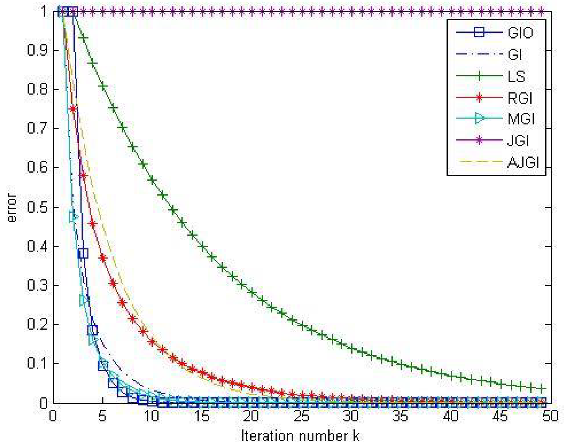
Example 1.

Consider the matrix equation $A_{1}X{B}_1+A_{2}X{B}_2+A_{3}X{B}_3=F$ when $A_1,A_2,A_3\in {\mathbb{R}}^{40\times 60}$, $B_1,B_2,B_3\in {\mathbb{R}}^{20\times 30}$ and $F\in {\mathbb{R}}^{40\times 30}$ are tridiagonal matrices given by

$$\begin{array}{cc}\hfill A_1& =tridiag(-2,2,-2),A_2=tridiag(2,-2,5),A_3=tridiag(2,-1,2),\hfill \\ \hfill B_1& =tridiag(4,3,-1),B_2=tridiag(1,-2,-1),B_3=tridiag(3,1,3).\hfill \end{array}$$

Here, the exact solution is given by $X=tridiag(1,-1,1)$. We apply Method 3 to compute the sequence $X\left(k\right)$ of approximated solutions. Take initial point

$$\begin{array}{c}\hfill X\left(0\right)={10}^{-6}\times tridiag(1,1,1).\end{array}$$

The optimal convergent factor can be computed as follows:

$${\tau }_{opt}=\frac{2}{{\lambda }_{min}\left(P^{T}P\right)+{\lambda }_{max}\left(P^{T}P\right)}\approx \frac{2}{4.15\times {10}^{-13}+1009.74}\approx 0.0019806.$$

The effect of changing convergent factors τ is illustrated in Figure 1. We see that as k large enough, the relative error ${\parallel E\left(k\right)\parallel }_F/{\parallel F\parallel }_F$ for ${\tau }_{opt}$ goes faster to 0 than for other convergent factors. If τ does not satisfy the condition (10), then the approximated solutions diverge for the given initial matrices. Moreover,

Table 1. Iteration numbers and computational times for Example 1.

Method	IT	CT
Direct	-	3.1380
GIO	161	0.0413
GI ($\tau =0.0001$)	3061	0.2508
GI ($\tau =0.00003$)	10,204	0.8994

shows that the computational time of our algorithm (GIO) is significantly less than the time of the direct method. Table 1 also demonstrates that, when we fix the error ${∥E\left(k\right)∥}_F$ to be less than $5\times {10}^{-3}$, the GIO algorithm outperforms another GI algorithms with different convergent factors in both iteration numbers and computational times.

Example 2.

Consider the matrix equation $A_{1}X{B}_1+A_{2}X{B}_2+A_{3}X{B}_3=F$ where all matrices are $100\times 100$ tridiagonal matrices given by

$$\begin{array}{cc}\hfill A_1& =tridiag(1,2,1),A_2=tridiag(-1,-2,-1),A_3=tridiag(-1,3,-1),\hfill \\ \hfill B_1& =tridiag(2,2,3),B_2=tridiag(1,2,-2),B_3=tridiag(3,2,-1).\hfill \end{array}$$

Here, the exact solution is $X=tridiag(1,1,1)$. To apply Method 3, we take initial matrix

$$\begin{array}{c}\hfill X\left(0\right)={10}^{-6}\times tridiag(0,2,0).\end{array}$$

We can compute ${\tau }_{opt}\approx 0.002553.$ Figure 2 shows that the relative error ${∥E\left(k\right)∥}_F/{∥F∥}_F$ for ${\tau }_{opt}$ goes faster to 0 than for other convergent factors. If τ does not satisfy (10), then the approximate solutions diverge for the given initial matrices. From

Table 2. Iteration numbers and computational times for Example 2.

Method	IT	CT
Direct	-	53.4063
GIO	389	0.5439
GI ($\tau =0.00005$)	19,314	28.0245
GI ($\tau =0.000001$)	96,557	148.4039

, we see that the computational time of our algorithm is significantly less than the time of the direct method. Furthermore, when the satisfactory error ${∥E\left(k\right)∥}_F$ is less than $ϵ=0.5$, the GIO algorithm has more efficiency than another GI algorithms in both iteration numbers and computational times.

Example 3.

Consider the Sylvester equation $AX+XB=F$, where $A,X,B,F\in {\mathbb{R}}^{10\times 10}$ are given by $A=tridiag(-1,3,1),B=tridiag(-3,2,3),X=tridiag(-3,1,4).$ We compare the efficiency of our method (GIO) with another iterative methods such as GI, LS, RGI, MGI, JGI and AJGI. We choose the same convergent factor $\tau =0.01836$ and the same initial matrix $X\left(0\right)=tridiag(0,{10}^{-6},0)$. To compare the efficiency of these methods, we fix the iteration number to be 50 and consider the relative errors ${\parallel E\left(k\right)\parallel }_F/{\parallel F\parallel }_F$. The results are displayed in Figure 3. The iteration numbers and the computational times when we fix the error ${\parallel E\left(k\right)\parallel }_F$ to be less than $5\times {10}^{-3}$ are illustrated in

Table 3. Iteration numbers and computational times for Example 3.

Method	GIO	GI	LS	RGI	MGI	JGI	AJGI	Direct
IT	18	33	167	70	25	-	51	-
CT	0.000273	0.000589	0.0114	0.0012	0.000789	-	0.0014	0.1704

. We see that our method is outperform to the direct method and another iterative methods with less iteration number and lower computational time. In particular, the approximated solutions generated from JGI method diverge.

6. An Application to Discretization of the Convection-Diffusion Equation

In this section, we apply the GIO method to a discretization of convection–diffusion equation in the form

$$\frac{\partial u}{\partial t}+\mu \frac{\partial u}{\partial x}=\alpha \frac{{\partial }^{2}u}{\partial x^2}\mathrm{for}c\le x\le d\mathrm{and}0\le t\le L$$

(22)

where $\mu$ and $\alpha$ are the convection and diffusion coefficients, respectively. Equation (22) is accompanied by the initial condition $u(x,0)=f\left(x\right)$ and boundary conditions $u(c,t)=g\left(t\right),u(d,t)=h\left(t\right)$ where $f,g,h$ are given functions. To make a discretization of Equation (22), we divide $[c,d]$ into M subintervals, each of equal length $h=(d-c)/M.$ In the same manner, we define a grid for the N subintervals $l=L/N.$ Then we make discretization at the grid point $u_m^n=u(x_m,t_n)$ where

$$x_m=c+mh\mathrm{and}{t}_n=nl$$

(23)

for $1\le m\le M$ and $1\le n\le N.$ By applying the forward time central space method, we have

$$(\frac{u_m^{n+1}-u_m^n}{l})+\mu (\frac{u_{m+1}^n-u_{m-1}^n}{2h})=\alpha (\frac{u_{m-1}^n-2u_m^n+u_{m+1}^n}{h^2}).$$

Rearranging the above equation leads to

$$u_m^{n+1}=(p+\frac{1}{2}r)u_{m-1}^n+(1-2p)u_m^n+(p-\frac{1}{2}r)u_{m+1}^n$$

where $r=\mu l/n$ and $p=\alpha l/h^2$ are the convection and diffusion numbers, respectively. We can transform (22) into a linear system of $MN$ unknowns $u_{11},\dots ,u_{MN}$ in the form

$$P_{CD}vec\left(U\right)=b,$$

(24)

where $U=\left[u_m^n\right],P_{CD}\in {\mathbb{R}}^{M\times N}$ has $N\times N$ blocks of the form $I_M$ on its diagonal and $tridiag(-p-\frac{1}{2}r,-1+2p,-p+\frac{1}{2}r)$ under its diagonal. The vector b is partitioned in M blocks as ${[b_1^T{b}_2^T\dots b_N^T]}^T$ where $b_1={\left[\begin{array}{c}\varphi \left(1\right)\varphi \left(2\right)\cdots \varphi (m-1)\end{array}\right]}^T$ and

$$b_j=\left[\begin{array}{c}(p+\frac{1}{2}r)g(t+(i-1)l)\\ 0\\ ⋮\\ 0\\ (p-\frac{1}{2}r)h(t+(i-1)l)\end{array}\right],j=2,\dots ,N$$

(25)

here $\varphi \left(i\right)=(p+\frac{1}{2}r)f(c+(i-1)h)+(1-2p)f(c+ih)+(p-\frac{1}{2}r)f(c+(i+1)h)$

We can see that Equation (24) is the generalized Sylvester equation where $p=1$, $A=P_{CD}$, $X=vec\left(U\right)$, $B=I$ and $F=b$. From Method 3, we obtain the following:

Method 5.

Input $M,N\in \mathbb{N}$ as number of partition. Set $P_{CD}^{\prime }=P_{CD}^T$.

Initializing step: Choose $u\left(0\right)\in {\mathbb{R}}^{MN}$. For each $m=1,2,\dots ,M$ and $n=1,2,\dots ,N$, compute $x_m$, $t_n$ as in Equation (23) and

$${\tau }_{opt}=\frac{2}{{\lambda }_{max}\left(P_{CD}^T{P}_{CD}\right)+{\lambda }_{min}\left(P_{CD}^T{P}_{CD}\right)}.$$

Updating step: For $k=1$ to end, do:

$$\begin{array}{cc}\hfill E(k-1)& =b-P_{CD}u(k-1),\hfill \\ \hfill u\left(k\right)& =\frac{1}{p}\sum _{i=1}^p(u(k-1)+{\tau }_{opt}{P}_{CD}^{\prime }E(k-1)).\hfill \end{array}$$

To stop the method, one may impose a stopping rule such as ${\parallel E\left(k\right)\parallel }_F/{\parallel b\parallel }_F<ϵ$ where ϵ is a tolerance error.

Now, we provide a numerical experiment for a convection-diffusion equation.

Example 4.

Consider the convection–diffusion equation

$$\frac{\partial u}{\partial t}+0.1\frac{\partial u}{\partial x}=0.01\frac{{\partial }^{2}u}{\partial x^2}for0\le x\le 1and0\le t\le 10$$

(26)

with the initial and boundary conditions given as:

$$u(x,0)=100xandu(0,t)=u(1,t)=0.$$

Let $M=5,N=10$, so that $P_{CD}$ is of dimension $50\times 50$. In this case, we have $h=0.2,l=1,r=0.5$ and $p=0.25.$ We choose $u\left(0\right)={10}^{-6}\left[\begin{array}{c}1\cdots 1\end{array}\right]\in {\mathbb{R}}^{50}.$

After compiling Method 5 for 100 iterations, we see from Figure 4 that the relative error ${∥E\left(k\right)∥}_F$ goes faster to 0 than for other methods such as GI, LS, RGI, MGI, JGI and AJGI. Moreover,

Table 4. Iteration numbers, computational times and errors for Example 4.

Method	IT	CT	Error
Direct	-	2.085	0
GIO	100	0.0113	0.0199
GI	100	0.0281	0.0648
LS	100	0.0469	1.6574
RGI	100	0.0324	0.1417
MGI	100	0.0313	0.0397
JGI	100	0.2813	0.7698
AJGI	100	0.0938	0.0307

displays comparison of numerical and direct solutions for the convection–diffusion equation.

A particular case $\mu =0$ of Equation (22) is called the diffusion equation. In this case, the formulas of $P_{CD}$ and $b_1,\dots ,b_N$ are reduced as $r=0.$

Example 5.

Consider the diffusion equation

$$\frac{\partial u}{\partial t}=\frac{{\partial }^{2}u}{\partial x^2}for0\le x\le 1and0\le t\le 10$$

with the initial and boundary conditions given as:

$$u(x,0)=6sin\left(\pi x\right)andu(0,t)=u(1,t)=0.$$

(27)

The exact solution is

$$u^{*}(x,t)=6e^{-{\pi }^{2}t}sin\left(\pi x\right).$$

Let $M=10,l=0.01$ In this case, we have $h=0.1,$ and $p=1.$ We choose initial matrix $u\left(0\right)={10}^{-6}\left[\begin{array}{c}1\cdots 1\end{array}\right]\in {\mathbb{R}}^{100}.$

After compiling Method 5 for 200 iterations (Figure 5), we see that our method is outperform to another iterative methods with less iteration number and lower computational time. The 3D-plot in Figure 6 shows that the iterative solution is well approximated to the exact solution.

7. Conclusions

We propose a gradient-based iterative method with an optimal convergent factor for solving a generalized Sylvester matrix equation. The convergence analysis reveals that the sequence of approximated solutions converge to the exact solution for any initial value if and only if the convergent factor is chosen properly. The convergent rate and error estimations depend on the spectral radius of the associated iteration matrix. Moreover, we obtain the fastest convergent factor so that the associated iteration matrix has the smallest spectral radius. Furthermore, the proposed algorithm is applicable for the discretization of the diffusion equations. The numerical experiments illustrate that our method is applicable for any conformable square/rectangular matrices of small/large sizes. Moreover, they reveal that our method performs well comparing to recent iterative methods.