Modified Jacobi-Gradient Iterative Method for Generalized Sylvester Matrix Equation

Abstract

We propose a new iterative method for solving a generalized Sylvester matrix equation $A_{1}X{A}_2+A_{3}X{A}_4=E$ with given square matrices $A_1,A_2,A_3,A_4$ and an unknown rectangular matrix X. The method aims to construct a sequence of approximated solutions converging to the exact solution, no matter the initial value is. We decompose the coefficient matrices to be the sum of its diagonal part and others. The recursive formula for the iteration is derived from the gradients of quadratic norm-error functions, together with the hierarchical identification principle. We find equivalent conditions on a convergent factor, relied on eigenvalues of the associated iteration matrix, so that the method is applicable as desired. The convergence rate and error estimation of the method are governed by the spectral norm of the related iteration matrix. Furthermore, we illustrate numerical examples of the proposed method to show its capability and efficacy, compared to recent gradient-based iterative methods.

1. Introduction

In control engineering, certain problems concerning the analysis and design of control systems can be formulated as the Sylvester matrix equation:

$$\begin{array}{c}\hfill A_{1}X+X{A}_2=C\end{array}$$

(1)

where $X\in {\mathbb{R}}^{m\times n}$ is an unknown matrix, and $A_1,A_2,C$ are known matrices of appropriate dimensions. Here, ${\mathbb{R}}^{m\times n}$ stands for the set of $m\times n$ real matrices. Let us denote by ${(·)}^T$ the transpose of a matrix. When $A_2={A_1}^T$, the equation is reduced to the Lyapunov equation, which is often found in continuous- and discrete-time stability analysis [1,2]. The Sylvester equation is a special case of a generalized Sylvester matrix equation:

$$\begin{array}{c}\hfill A_{1}X{A}_2+A_{3}X{A}_4=E\end{array}$$

(2)

where $X\in {\mathbb{R}}^{m\times n}$ is unknown, and $A_1,A_2,A_3,A_4,E$ are known constant matrices of appropriate dimensions. This equation also includes the equation $A_{1}X{A}_2=C$ and the Kalman–Yakubovich equation $A_{1}X{A}_2-X=C$ as special cases. All of these equations have profound applications in linear system theory and related areas.

Normally, a direct way to solve the generalized Sylvester Equation (2) is to reduce it to a linear system by taking the vector operator. Then, Equation (2) reduces to $Px=b$ where

$$P={A_2}^T\otimes A_1+{A_4}^T\otimes A_3,x=vec\left(X\right),\mathrm{and}b=vec\left(E\right).$$

Here, $vec(·)$ is the vector operator and the operation ⊗ is the Kronecker multiplication. So, Equation (2) has a unique solution if and only if the square matrix P is invertible. However, it is not easy to compute $P^{-1}$ when the sizes of $A_1,A_2,A_3,A_4$ are not small, since the size of P can be very large. Such a size problem leads to computation difficulty in that excessive computer memory is required for the inversion of large matrices. Thus, another way exists which transform the matrix cofficients into a Schur or Hessenberg form, for which solutions may be readily computed—see [3,4].

For matrix equations of large dimensions, iterative algorithms to find an approximated/exact solution are remarkable. There are many techniques to construct an iterative procedure for Equation (2) or its special cases—e.g., matrix sign function [5], block successive over-relaxation [6], block recursion [7,8], Krylov subspace [9,10], and truncated low-rank algorithm [11]. Lately, there have been some variants of Hermitian and skew-Hermitian splitting—e.g., a generalized modified Hermitian and skew-Hermitian splitting algorithm [12], accelerated double-step scale splitting algorithm [13], PHSS algorithm [14], and the four parameter PSS algorithm [15]. Furthermore, the idea of conjugate gradient leads to finite-step iterative methods to find the exact solution such as the generalized conjugated direction algorithm [16], the conjugated gradient least-squares algorithm [17], and generalized product-type methods based on the Bi-conjugate gradient algorithm [18].

In the last decade, many authors have developed gradient-based iterative (GI) algorithms for certain linear matrix equations that satisfy the asymptotic stability (AS) in the following meaning:

(AS): The sequence of approximated solutions converges to the exact solution, no matter the initial value is.

The first GI algorithm for solving (1) was developed by Ding and Chen [19]. In that paper, a sufficient condition in terms of a convergence factor is determined so that the algorithm satisfies (AS) property. By introducing of a relaxation parameter, Niu et al. [20] suggested a relaxed gradient iterative (RGI) gradient algorithm to overcome (1). Numerical studies show that when the relaxation factor is correctly selected the convergent behavior of the Niu’s algorithm is stronger than the Ding’s algorithm. Zhang and Sheng [21] introduced an RGI algorithm for finding the symmetric (skew-symmetric) solution of Equation (1). Xie et al. [22] improved the RGI algorithm to become an accelerated GI (AGBI) algorithm, on the basis of the information generated in the previous half-step and a relaxation factor. Ding and Chen [23] also applied the ideas of gradients and least-squares to formulate the least-squares iterative (LSI) algorithm. In [24], Fan et al. realized that multiplication of the matrix in GI would take great time and space if $A_1$ and $A_2$ were big and dense, so they proposed the following Jacobi-gradient iterative (JGI) method.

Method 1

(Jacobi-Gradient based Iterative (JGI) algorithm [24]). For $i=1,2$, let $D_i$ be the diagonal part of $A_i$. Given any initial matrices $X_1\left(0\right),X_2\left(0\right)$. Set $k=0$ and compute $X\left(0\right)=(1/2)(X_1\left(0\right)+X_2\left(0\right))$. For $k=1,2,\dots ,End$, do:

$$\begin{array}{cc}\hfill X_1\left(k\right)& =X(k-1)+\mu D_1[C-A_{1}X(k-1)-X(k-1)A_2],\hfill \\ \hfill X_2\left(k\right)& =X(k-1)+\mu [C-A_{1}X(k-1)-X(k-1)A_2]D_2,\hfill \\ \hfill X\left(k\right)& =\frac{1}{2}(X_1\left(k\right)+X_2\left(k\right)).\hfill \end{array}$$

After that, Tian et al. [25] proposed that an accelerated Jacobi-gradient iterative (AJGI) algorithm for solving the Sylvester matrix equation relies on two relaxation factors and the half-step update. However, the parameter values to apply to the algorithm are difficult to find since they are given in terms of a nonlinear inequality. For the generalized Sylvester Equation (2), the gradient iterative (GI) algorithm [19] and the least-squares iterative (LSI) algorithm [26] were established as follows.

Method 2

(GI algorithm [19]). Given any two initial matrices $X_1\left(0\right),X_2\left(0\right)$. Set $k=0$ and compute $X\left(0\right)=(1/2)(X_1\left(0\right)+X_2\left(0\right))$. For $k=1,2,\dots ,End$, do:

$$\begin{array}{cc}\hfill X_1\left(k\right)& =X(k-1)+\mu A_1^T[E-A_{1}X(k-1)A_2-A_{3}X(k-1)A_4]A_2^T,\hfill \\ \hfill X_2\left(k\right)& =X(k-1)+\mu A_3^T[E-A_{1}X(k-1)A_2-A_{3}X(k-1)A_4]A_4^T,\hfill \\ \hfill X\left(k\right)& =\frac{1}{2}(X_1\left(k\right)+X_2\left(k\right)).\hfill \end{array}$$

A sufficient condition for which the algorithm satisfies (AS) is

$$\begin{array}{c}\hfill 0<\mu <\frac{2}{\Vert A_1{\Vert }_2^2\Vert A_2{\Vert }_2^2+\Vert A_3{\Vert }_2^2{\Vert A_4\Vert }_2^2}.\end{array}$$

Method 3

(LSI algorithm [26]). Given any two initial matrices $X_1\left(0\right), X_2\left(0\right)$. Set $k=0$ and compute $X\left(0\right)=\frac{1}{2}(X_1\left(0\right)+X_2\left(0\right))$. For $k=1,2,\dots ,End$, do:

$$\begin{array}{cc}\hfill X_1\left(k\right)& =X(k-1)+\mu {\left(A_1^T{A}_1\right)}^{-1}{A}_1^T[E-A_{1}X(k-1)A_2-A_{3}X(k-1)A_4]A_2^T{\left(A_2{A}_2^T\right)}^{-1},\hfill \\ \hfill X_2\left(k\right)& =X(k-1)+\mu {\left(A_3^T{A}_3\right)}^{-1}{A}_3^T[E-A_{1}X(k-1)A_2-A_{3}X(k-1)A_4]A_4^T{\left(A_4{A}_4^T\right)}^{-1},\hfill \\ \hfill X\left(k\right)& =\frac{1}{2}(X_1\left(k\right)+X_2\left(k\right)).\hfill \end{array}$$

If $0<\mu <4$, then the algorithm satisfies (AS).

In this paper, we shall propose a new iterative method for solving the generalized Sylvester matrix Equation (2), when $A_1,A_3\in {\mathbb{R}}^{m\times m}$, $A_2,A_4\in {\mathbb{R}}^{n\times n}$ and $X,E\in {\mathbb{R}}^{m\times n}$. This algorithm requires only one initial value $X\left(0\right)$ and only one parameter, called a convergence factor. We decompose the coefficient matrices to be the sum of its diagonal part and others. The recursive formula for iteration is derived from the gradients of quadratic norm-error functions together with hierarchical identification principle. Under assumptions on the real-parts sign of eigenvalues of matrix coefficients, we find necessary and sufficient conditions on a convergent factor for which (AS) holds. The convergence rate and error estimates are regulated by the iteration matrix spectral radius. In particular, when the iteration matrix is symmetric, we obtain a convergence criteria, error estimates and the optimal convergent factor in terms of spectral norms and condition number. Moreover, numerical simulations are also provided to illustrate our results for (2) and (1). We compare the efficiency of our algorithm to LSI, GI, RGI, AGBI and JGI algorithms.

Let us recall some terminology from matrix analysis—see e.g., [27]. For any square matrix X, denote $\sigma \left(X\right)$ its spectrum, $\rho \left(X\right)$ its spectral radius, and $tr\left(X\right)$ its trace. Let us denote the largest and the smallest eigenvalues of a matrix by ${\lambda }_{max}(·)$ and ${\lambda }_{min}(·)$, respectively. Recall that the spectral norm ${\Vert ·\Vert }_2$ and the Frobenius norm ${\Vert ·\Vert }_F$ of $A\in {\mathbb{R}}^{m\times n}$ are, respectively, defined by

$$\begin{array}{c}\hfill {\Vert A\Vert }_2=\sqrt{{\lambda }_{max}\left(A^{T}A\right)}\mathrm{and}{\Vert A\Vert }_F=\sqrt{tr\left(A^{T}A\right)}.\end{array}$$

The condition number of $A\ne 0$ is defined by

$$\kappa \left(A\right)=\sqrt{\frac{{\lambda }_{max}\left(A^{T}A\right)}{{\lambda }_{min}\left(A^{T}A\right)}}.$$

Denote the real part of a complex number z by $\Re \left(z\right)$.

The rest of paper is organized as follows. We propose a modified Jacobi-gradient iterative algorithm in Section 2. Convergence criteria, convergence rate, error estimates, and optimal convergence factor are discussed in Section 3. In Section 4, we provide numerical simulations of the algorithm. Finally, we conclude the paper in Section 5.

2. A Modified Jacobi-Gradient Iterative Method for the Generalized Sylvester Equation

In this section, we propose an iterative algorithm for solving the generalized Sylvester equation, called a modified Jacobi-gradient iterative algorithm.

Throughout, let $m,n\in \mathbb{N}$ and $A_1,A_3\in {\mathbb{R}}^{m\times m}$, $A_2,A_4\in {\mathbb{R}}^{n\times n}$ and $E\in {\mathbb{R}}^{m\times n}$. We would like to find a matrix $X\in {\mathbb{R}}^{m\times n}$, such that

$$\begin{array}{c}\hfill A_{1}X{A}_2+A_{3}X{A}_4=E.\end{array}$$

(3)

Write $A_1=D_1+F_1,A_2=D_2+F_2,A_3=D_3+F_3\mathrm{and}{A}_4=D_4+F_4$, where $D_1,D_2,D_3,D_4$ are the diagonal parts of $A_1,A_2,A_3,A_4$, respectively. A necessary and sufficient condition for (3) to have a unique solution is the invertibility of the square matrix

$$P:=A_2^T\otimes A_1+A_4^T\otimes A_3.$$

In this case, the solution is given by $vecX=P^{-1}vecE$.

To obtain an iterative algorithm for solving (3), we recall the hierarchical identification principle in [19]. We write (3) to

$$\begin{array}{cc}\hfill (D_1+F_1)X(D_2+F_2)+A_{3}X{A}_4& =E,\hfill \end{array}$$

(4)

$$\begin{array}{cc}\hfill A_{1}X{A}_2+(D_3+F_3)X(D_4+F_4)& =E.\hfill \end{array}$$

(5)

Define two matrices

$$M:=E-F_{1}X{D}_2-D_{1}X{F}_2-F_{1}X{F}_2-A_{3}X{A}_4,$$

$$N:=E-F_{3}X{D}_4-D_{3}X{F}_4-F_{3}X{F}_4-A_{1}X{A}_2.$$

From (4) and (5), we shall find the approximated solution of the following two subsystems

$$\begin{array}{c}\hfill D_{1}X{D}_2=M\mathrm{and}{D}_{3}X{D}_4=N\end{array}$$

(6)

so that the following norm-error functions are minimized:

$$\begin{array}{c}\hfill L_1\left(X\right):=\Vert D_{1}X{D}_2{-M\Vert }_F^2\mathrm{and}{L}_2\left(X\right):={\Vert D_{3}X{D}_4-N\Vert }_F^2.\end{array}$$

(7)

From the gradient formula

$$\begin{array}{c}\hfill \frac{d}{dX}tr\left(AX\right)=A^T,\end{array}$$

we can deduce the gradient of the error $L_1$ as follows:

$$\begin{array}{cc}\hfill \frac{\partial }{\partial X}{L}_1\left(X\right)& =\frac{\partial }{\partial X}tr\left[{(D_{1}X{D}_2-M)}^T(D_{1}X{D}_2-M)\right]\hfill \\ \hfill & =\frac{\partial }{\partial X}tr\left(X{D}_2{D}_2{X}^T{D}_1{D}_1\right)-\frac{\partial }{\partial X}tr\left(X{D}_2{M}^T{D}_1\right)-\frac{\partial }{\partial X}tr\left(X^T{D}_{1}M{D}_2\right)\hfill \\ \hfill & =\left(D_1{D}_2\right)X^T{D}_2{D}_2+D_1{D}_{1}X{D}_2{D}_2-D_{1}M{D}_2-{\left(D_2{M}^T{D}_1\right)}^T\hfill \\ \hfill & =2D_1(D_{1}X{D}_2-M)D_2.\hfill \end{array}$$

(8)

Similarly, we have

$$\begin{array}{c}\hfill \frac{\partial }{\partial X}{L}_2\left(X\right)=2A_3^T(A_{3}X{A}_4-N)A_4^T.\end{array}$$

(9)

Let $X_1\left(k\right)$ and $X_2\left(k\right)$ be the estimates or iterative solutions of the system (6) at k-th iteration. The recursive formulas of $X_1\left(k\right)$ and $X_2\left(k\right)$ come from the gradient formulas (8) and (9), as follows:

$$\begin{array}{cc}\hfill X_1\left(k\right)& =X(k-1)+\mu D_1(M-D_{1}X(k-1)D_2)D_2\hfill \\ \hfill & =X(k-1)+\mu D_1(E-A_{1}X(k-1)A_2+A_{3}X(k-1)A_4)D_2,\hfill \\ \hfill X_2\left(k\right)& =X(k-1)+\mu D_3(N-D_{3}X(k-1)D_3)D_4\hfill \\ \hfill & =X(k-1)+\mu D_3(E-A_{1}X(k-1)A_2+A_{3}X(k-1)A_4)D_4.\hfill \end{array}$$

Based on the hierarchical identification principle, the unknown variable X is replaced by its estimates at the $(k-1)$-th iteration. To avoid duplicated computation, we introduce a matrix

$$S\left(k\right)=E-(A_{1}X\left(k\right)A_2+A_{3}X\left(k\right)A_4),$$

so we have

$$\begin{array}{c}\hfill X\left(k\right)=\frac{1}{2}(X_1\left(k\right)+X_2\left(k\right))=X(k-1)+\mu (D_{1}S(k-1)D_2+D_{3}S(k-1)D_4).\end{array}$$

(10)

Since any diagonal matrix is sparse, the operation counts in the computation (10) can be substantially reduced. Let us denote $S\left(k\right)=\left[s_{ij}\left(k\right)\right]$, $X\left(k\right)=\left[x_{ij}\left(k\right)\right]$, and $D_l=[d_{ij}^{\left(l\right)}]$ for each $l=1,2,3,4$. Indeed, the multiplication of $D_{1}S\left(k\right)D_2$ results in a matrix whose $\left(ij\right)$-th entry is the product of the i-th entry in the diagonal of $D_1$, the $\left(ij\right)$-th entry of $S\left(k\right)$, and the j-th entry of $D_2$—i.e., $D_{1}S\left(k\right)D_2=[d_{ii}^{\left(1\right)}{s}_{ij}\left(k\right)d_{jj}^{\left(2\right)}]$. Similarly, $D_{3}S\left(k\right)D_4=[d_{ii}^{\left(3\right)}{s}_{ij}\left(k\right)d_{jj}^{\left(4\right)}]$. Thus,

$$D_{1}S\left(k\right)D_2+D_{3}S\left(k\right)D_4=[(d_{ii}^{(1)}{d}_{jj}^{(2)}+d_{ii}^{(3)}{d}_{jj}^{(4)})s_{ij}(k)].$$

The above discussion leads to the following Algorithm 1.

Algorithm 1: Modified Jacobi-gradient based iterative (MJGI) algorithm

The complexity analysis for each step of the algorithm is given by $2mn(m+n+5)$. When $m=n$, the complexity analysis is $4n^3+10n^2\in O\left(n^3\right)$, so that the algorithm runtime complexity is cubic time. The convergence property of the algorithm relies on the convergence factor $\mu$. The appropriate value of this parameter is determined in the next section.

3. Convergence Analysis of the Proposed Method

In this section, we make convergence analysis of Algorithm 1. First, we transform it into a linear iterative method of the first order: $x\left(k\right)=Tx(k-1)$ where $x\left(k\right)$ is a vector variable and T is a matrix. The iteration matrix T will reflect convergence criteria, convergence rate, and error estimates of the algorithm.

3.1. Convergence Criteria

Theorem 1.

Assume that the generalized Sylvester matrix Equation (3) has a unique solution$X^{*}$. Denote$H=\mathfrak{D}\left(P\right)P$and write$\sigma \left(H\right)=\left\{{\lambda }_1,\dots ,{\lambda }_{mn}\right\}$. Let$\left\{X\right(k\left)\right\}$be a sequence generated from Algorithm 1.

(1)

Then, (AS) holds if and only if$\rho (I_{mn}-\mu H)<1$.

(2)

If$\Re \left({\lambda }_j\right)>0$for all$j=1,\dots ,mn$, then (AS) holds if and only if

$$\begin{array}{c}\hfill 0<\mu <\underset{j=1,\dots ,mn}{max}\frac{2\Re \left({\lambda }_j\right)}{{|{\lambda }_j|}^2}.\end{array}$$

(3)

If$\Re \left({\lambda }_j\right)<0$for all$j=1,\dots ,mn$, then (AS) holds if and only if

$$\begin{array}{c}\hfill \underset{j=1,\dots ,mn}{min}\frac{2\Re \left({\lambda }_j\right)}{{|{\lambda }_j|}^2}<\mu <0.\end{array}$$

(4)

If H is symmetric, then (AS) holds if and only if${\lambda }_{max}\left(H\right)$and${\lambda }_{min}\left(H\right)$have the same sign, and μ is chosen so that

$$\left\{\begin{array}{cc}0<\mu <\frac{2}{{\lambda }_{max}\left(H\right)}\hfill & \mathit{if}{\lambda }_{min}\left(H\right)>0,\hfill \\ \frac{2}{{\lambda }_{min}\left(H\right)}<\mu <0\hfill & \mathit{if}{\lambda }_{max}\left(H\right)<0.\hfill \end{array}\right.$$

Proof. 

From Algorithm 1, we start with considering the error matrices

$$\tilde{X}\left(k\right)=X\left(k\right)-X^{*},{\tilde{X}}_1\left(k\right)=X_1\left(k\right)-X^{*}\mathrm{and}{\tilde{X}}_2\left(k\right)=X_2\left(k\right)-X^{*}.$$

We will show that $\tilde{X}\left(k\right)\to 0,$ or equivalently, $vec\tilde{X}\left(k\right)\to 0$ as $k\to \infty$. A direct computation reveals that

$$\begin{array}{cc}\hfill \tilde{X}\left(k\right)& =\frac{1}{2}(X_1\left(k\right)+X_2\left(k\right))\hfill \\ \hfill & =\tilde{X}(k-1)-\frac{1}{2}\mu D_1(A_1\tilde{X}(k-1)A_2+A_3\tilde{X}(k-1)A_4)D_2\hfill \\ \hfill & -\frac{1}{2}\mu D_3(A_1\tilde{X}(k-1)A_2+A_3\tilde{X}(k-1)A_4)D_4.\hfill \end{array}$$

By taking the vector operator and using properties of the Kronecker product, we have

$$\begin{array}{ccc}\hfill vec\tilde{X}(k)& =vec\tilde{X}(k-1)\hfill & \hfill \\ \hfill & -\mu vec(D_1{A}_1\tilde{X}(k-1)A_2{D}_2+D_1{A}_3\tilde{X}(k-1)A_4{D}_2)\hfill \\ \hfill & -\mu vec(D_3{A}_1\tilde{X}(k-1)A_2{D}_4+D_3{A}_3\tilde{X}(k-1)A_4{D}_4)\hfill \\ \hfill & =\{I_{mn}-\mu [(D_2\otimes D_1)(A_2^T\otimes A_1)(+D_2\otimes D_1)(A_4^T\otimes A_3)\hfill \\ \hfill & +(D_4\otimes D_3)(A_2^T\otimes A_1)+(D_4\otimes D_3)(A_4^T\otimes A_3)\left]\right\}vec(\tilde{X}(k-1))\hfill \\ \hfill & =[I_{mn}-\mu (D_2\otimes D_1+D_4\otimes D_3)(A_2^T\otimes A_1+A_4^T\otimes A_3)]vec(\tilde{X}(k-1)).\hfill \end{array}$$

Let us denote the diagonal part of P by $\mathfrak{D}\left(P\right)$. Indeed,

$$\begin{array}{c}\hfill \mathfrak{D}\left(P\right)=D_2\otimes D_1+D_4\otimes D_3.\end{array}$$

Thus, we arrive at a linear iterative process

$$\begin{array}{cc}\hfill vec\tilde{X}\left(k\right)& =[I_{mn}-\mu H]vec\tilde{X}(k-1),\hfill \end{array}$$

(11)

where $H=\mathfrak{D}\left(P\right)P$. Hence, the following statements are equivalent:

(i)

$vec\tilde{X}\left(k\right)\to 0$ for any initial value $vec\tilde{X}\left(0\right)$.

(ii)

System (11) has an asymptotically-stable zero solution.

(iii)

The iteration matrix $I_{mn}-\mu H$ has spectral radius less than 1.

Indeed, since $I_{mn}-\mu H$ is a polynomial of H, we get

$$\begin{array}{c}\hfill \rho (I_{mn}-\mu H)=\underset{\lambda \in \sigma \left(H\right)}{max}|1-\mu \lambda |.\end{array}$$

(12)

Thus, $\rho (I_{mn}-\mu H)<1$ if and only if $|1-\mu \lambda |<1$ for all $\lambda \in \sigma \left(H\right)$. Write ${\lambda }_j=a_j+i{b}_j$ where $a_j,b_j\in \mathbb{R}$. It follows that the condition $|1-\mu {\lambda }_j|<1$ is equivalent to $(1-\mu {\lambda }_j)\overline{(1-\mu {\lambda }_j)}<1$, or

$$\begin{array}{c}\hfill \mu (-2a_j+\mu (a_j^2+b_j^2))<0.\end{array}$$

Thus, we arrive at two alternative conditions:

(i)

$\mu >0$ and $-2a_j+\mu (a_j^2+b_j^2)<0$ for all $j=1,2,3,\dots ,mn$;

(ii)

$\mu <0$ and $-2a_j+\mu (a_j^2+b_j^2)>0$ for all $j=1,2,3,\dots ,mn$.

Case 1

$a_j=\Re \left({\lambda }_j\right)>0$ for all j. In this case, $\rho (I_{mn}-\mu H)<1$ if and only if

$$\begin{array}{c}\hfill 0<\mu <\underset{j=1,\dots ,mn}{max}\frac{2a_j}{a_j^2+b_j^2}.\end{array}$$

(13)

Case 2

$a_j=\Re \left({\lambda }_j\right)<0$ for all j. In this case, $\rho (I_{mn}-\mu H)<1$ if and only if

$$\begin{array}{c}\hfill \underset{j=1,\dots ,mn}{min}\frac{2a_j}{a_j^2+b_j^2}<\mu <0.\end{array}$$

(14)

Now, suppose that H is a symmetric matrix. Then $I_{mn}-\mu H$ is also symmetric, and thus all its eigenvalue are real. Hence,

$$\begin{array}{c}\hfill \rho (I_{mn}-\mu H)=max\left\{|1-\mu {\lambda }_{min}\left(H\right)|,|1-\mu {\lambda }_{max}\left(H\right)|\right\}.\end{array}$$

(15)

It follows that $\rho (I_{mn}-\mu H)<1$ if and only if

$$\begin{array}{c}\hfill 0<\mu {\lambda }_{min}\left(H\right)<2\mathrm{and}0<\mu {\lambda }_{max}\left(H\right)<2.\end{array}$$

(16)

So, ${\lambda }_{min}\left(H\right)$ and ${\lambda }_{max}\left(H\right)$ cannot be zero.

Case 1

If ${\lambda }_{max}\left(H\right)\ge {\lambda }_{min}\left(H\right)>0,$ then the condition (16) is equivalent to

$$\begin{array}{c}\hfill 0<\mu <\frac{2}{{\lambda }_{max}\left(H\right)}.\end{array}$$

Case 2

If ${\lambda }_{min}\left(H\right)\le {\lambda }_{max}\left(H\right)<0,$ then the condition (16) is equivalent to

$$\begin{array}{c}\hfill \frac{2}{{\lambda }_{min}\left(H\right)}<\mu <0.\end{array}$$

Case 3

If ${\lambda }_{min}\left(H\right)<0<{\lambda }_{max}\left(H\right)$, then

$$\begin{array}{c}\hfill \frac{2}{{\lambda }_{min}\left(H\right)}<\mu <0\mathrm{and}0<\mu <\frac{2}{{\lambda }_{max}\left(H\right)},\end{array}$$

which is a contradiction.

Therefore, the condition (16) holds if and only if ${\lambda }_{max}\left(H\right)$ and ${\lambda }_{min}\left(H\right)$ have the same sign and $\mu$ is chosen according to the above condition. □

3.2. Convergence Rate and Error Estimate

We now discuss the convergence rate and error estimates of Algorithm 1 from the iterative process (11).

Suppose that Algorithm 1 satisfies the (AS) property—i.e., $\rho (I_{mn}-\mu H)<1$. From (11), we have

$$\begin{array}{cc}\hfill {\Vert X\left(k\right)-X^{*}\Vert }_F& ={\Vert vec\tilde{X}\left(k\right)\Vert }_F={\Vert (I_{mn}-\mu H)vec\tilde{X}(k-1)\Vert }_F\hfill \\ \hfill & \le {\Vert I_{mn}-\mu H\Vert }_2{\Vert \tilde{X}(k-1)\Vert }_F={\Vert I_{mn}-\mu H\Vert }_2{\Vert X(k-1)-X^{*}\Vert }_F.\hfill \end{array}$$

(17)

It follows inductively that for each $k\in \mathbb{N}$,

$$\begin{array}{c}\hfill {\Vert X\left(k\right)-X^{*}\Vert }_F\le {\Vert I_{mn}-\mu H\Vert }_2^k{\Vert X\left(0\right)-X^{*}\Vert }_F.\end{array}$$

(18)

Hence, the spectral norm of $I_{mn}-\mu H$ describes how fast the approximated solutions $X\left(k\right)$ converges to the exact solution $X^{*}$. The smaller spectral radius, the faster $X\left(k\right)$ goes to $X^{*}$. In that case, since ${\Vert I_{mn}-\mu H\Vert }_2<1$, if ${\Vert X(k-1)-X^{*}\Vert }_F\ne 0$ (i.e., $X(k-1)$ is not the exact solution) then

$$\begin{array}{c}\hfill {\Vert X\left(k\right)-X^{*}\Vert }_F<{\Vert X(k-1)-X^{*}\Vert }_F.\end{array}$$

(19)

Thus, the error at each iteration gets smaller than the previous one.

The above discussion is summarized in the following theorem.

Theorem 2.

Suppose that the parameter μ is chosen as in Theorem 1 so that Algorithm 1 satisfies (AS). Then, the convergence rate of the algorithm is governed by the spectral radius (16). Moreover, the error estimate ${\Vert X\left(k\right)-X^{*}\Vert }_F$ compared to the previous step and the fast step are provided by (17) and (18), respectively. In particular, the error at each iteration gets smaller than the $\left(nonzero\right)$ previous one, as in (19).

From (16), if the eigenvalues of $\mu H$ are close to 1, then the spectral radius of the iteration matrix is close to 0, and hence, the error $vec\tilde{X}\left(k\right)$ or $\tilde{X}\left(k\right)$ converge faster to 0.

Remark 1.

The convergence criteria and the convergence rate of Algorithm 1 depend on A, B, C and D but not on E. However, the matrix E can be used for the stopping criteria.

The next proposition determines the iteration number for which the approximated solution $X\left(k\right)$ is close to the exact solution $X^{*}$ so that ${\Vert X\left(k\right)-X^{*}\Vert }_F<ϵ$.

Proposition 1.

According to Algorithm 1, for each given error $ϵ>0$, we have ${\Vert X\left(k\right)-X^{*}\Vert }_F<ϵ$ after $k^{*}$ iterations for any $k^{*}$, such that

$$\begin{array}{c}\hfill k^{*}>\frac{logϵ-log{\Vert X\left(k\right)-X^{*}\Vert }_F}{log{\Vert I_{mn}-\mu H\Vert }_2}.\end{array}$$

(20)

Proof. 

From the estimation (18), we have

$$\begin{array}{c}\hfill {\Vert X\left(k\right)-X^{*}\Vert }_F\le {\Vert I_{mn}-\mu H\Vert }_2^k{\Vert X\left(0\right)-X^{*}\Vert }_F\to 0\mathrm{as}k\to \infty .\end{array}$$

This means precisely that for each given $ϵ>0$, there is a $k^{*}\in \mathbb{N}$ such that for all $k\ge k^{*}$,

$${\Vert I_{mn}-\mu H\Vert }_2^k{\Vert X\left(0\right)-X^{*}\Vert }_F<ϵ.$$

Taking logarithms, we have that the above condition is equivalent to (20). Thus, if we run Algorithm 1 $k^{*}$ times, then we get $\Vert X\left(k\right)-X^{*}\Vert <ϵ$ as desired. □

3.3. Optimal Parameter

We discuss the fastest convergence factor for Algorithm 1.

Theorem 3.

The optimal convergence factor μ for which Algorithm 1 satisfies (AS) is one that minimizes $\Vert I_{mn}{-\mu H\Vert }_2$. If, in addition, H is symmetric, then the optimal convergence factor for which the algorithm satisfies (AS) is determined by

$$\begin{array}{cc}\hfill {\mu }_{opt}& =\frac{2}{{\lambda }_{min}\left(H\right)+{\lambda }_{max}\left(H\right)}.\hfill \end{array}$$

(21)

In this case, the convergence rate is governed by

$$\begin{array}{c}\hfill \rho (I_{mn}-\mu H)=\frac{{\lambda }_{max}\left(H\right)-{\lambda }_{min}\left(H\right)}{{\lambda }_{max}\left(H\right)+{\lambda }_{min}\left(H\right)}=\frac{{\kappa }^2-1}{{\kappa }^2+1},\end{array}$$

(22)

where κ denotes be condition number of H, and we have the following estimates:

$$\begin{array}{cc}\hfill \Vert X\left(k\right)-X^{*}{\Vert }_F& \le \frac{{\kappa }^2-1}{{\kappa }^2+1}{\Vert X(k-1)-X^{*}\Vert }_F,\hfill \end{array}$$

(23)

$$\begin{array}{cc}\hfill \Vert X\left(k\right)-X^{*}{\Vert }_F& \le {\left(\frac{{\kappa }^2-1}{{\kappa }^2+1}\right)}^k{\Vert X\left(0\right)-X^{*}\Vert }_F.\hfill \end{array}$$

(24)

Proof. 

From Theorem 2, it is clear that the fastest convergence factor is attained at a convergence factor that minimizes $\Vert I_{mn}{-\mu H\Vert }_2$. Now, assume that H is symmetric. Then, $I_{mn}-\mu H$ is also symmetric, thus all its eigenvalues are real and

$$\begin{array}{c}\hfill {\Vert I_{mn}-\mu H\Vert }_2=\rho (I_{mn}-\mu H).\end{array}$$

(25)

For convenience, denote $a={\lambda }_{min}\left(H\right)$, $b={\lambda }_{max}\left(H\right)$, and

$$\begin{array}{c}\hfill f\left(\mu \right):=\rho (I_{mn}-\mu H)=max\left\{|1-\mu a|,|1-\mu b|\right\}.\end{array}$$

First, we consider the case ${\lambda }_{min}\left(H\right)>0$. To obtain the fastest convergence factor, according to (15), we must solve the following optimization problem

$$\begin{array}{c}\hfill \underset{0<\mu <\frac{2}{{\lambda }_{max}\left(H\right)}}{min}{\Vert I_{mn}-\mu H\Vert }_2=\underset{0<\mu <\frac{2}{b}}{min}f\left(\mu \right).\end{array}$$

We obtain that the minimizer is given by ${\mu }_{opt}=2/(a+b)$, so that $f\left({\mu }_{opt}\right)=(b-a)/(b+a)$. For the case ${\lambda }_{max}\left(H\right)<0$, we solve the following optimization problem

$$\begin{array}{c}\hfill \underset{\frac{2}{{\lambda }_{min}\left(H\right)}<\mu <0}{min}{\Vert I_{mn}-\mu H\Vert }_2=\underset{\frac{2}{a}<\mu <0}{min}f\left(\mu \right).\end{array}$$

A similar argument yields the same minimizer (21) and the same convergence rate (22). From (17), (18) and (25), we obtain the bounds (23) and (24). □

4. Numerical Simulations

In this section, we report numerical results to illustrate the effectiveness of Algorithm 1. We consider various sizes of matrix systems, namely, small $(2\times 2)$, medium $(10\times 10)$ and large $(100\times 100)$. For the generalized Sylvester equation, we compare the performance of Algorithm 1 to the GI and LSI algorithms. For the Sylvester equation, we compare our algorithm with GI, RGI, AGBI and JGI algorithms. All iterations have been carried out the same environment: MATLAB R2017b, Intel(R) Core(TM) i7-7660U CPU @ 2.5GHz, RAM 8.00 GB Bus speed 2133 MHz. We abbreviate IT and CPU for iteration time and CPU time (in seconds), respectively. As step k-th of the iteration, we consider the following error:

$$\begin{array}{c}\hfill \delta \left(k\right):={\Vert E-A_{1}X\left(k\right)A_2-A_{3}X\left(k\right)A_4\Vert }_F\end{array}$$

where $X\left(k\right)$ is the k-th approximated solution of the corresponding system.

4.1. Numerical Simulation for the Generalized Sylvester Matrix Equation

Example 1.

Consider the matrix equation $A_{1}X{A}_2+A_{3}X{A}_4=E$ where

$$\begin{array}{cc}\hfill A_1& =\left[\begin{array}{cc}0.6959& -0.6385\\ 0.6999& 0.0336\end{array}\right],A_2=\left[\begin{array}{cc}-0.0688& -0.5309\\ 0.3196& 0.6544\end{array}\right],A_3=\left[\begin{array}{cc}0.4076& 0.7184\\ -0.8200& 0.9686\end{array}\right],\hfill \\ \hfill A_4& =\left[\begin{array}{cc}0.5313& 0.1056\\ 0.3251& 0.6110\end{array}\right],E=\left[\begin{array}{cc}0.7788& 0.0908\\ 0.4235& 0.2665\end{array}\right].\hfill \end{array}$$

Then, the exact solution of X is

$$\begin{array}{c}\hfill X^{*}=\left[\begin{array}{cc}1.3036& -0.0532\\ 1.2725& 1.2284\end{array}\right].\end{array}$$

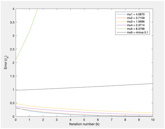
Choose $X\left(0\right)=zeros\left(2\right)$. In this case, all eigenvalues of H have positive real parts. The effect of changing the convergence factor μ is illustrated in Figure 1. According to Theorem 1, the criteria for the convergence of $X\left(k\right)$ is that $\mu \in (0,4.1870)$. Since ${\mu }_1,{\mu }_2,{\mu }_3,{\mu }_4$ satisfy this criteria, the error is becoming smaller and goes to zero as k increase, as in Figure 1. Among them, ${\mu }_4=4.0870$ gives the fastest convergence. For ${\mu }_5$ and ${\mu }_6$, which do not meet the criteria, the error $\delta \left(k\right)$ does not converge to zero.

Figure 1. Error of Example 1.

Example 2.

Suppose that $A_{1}X{A}_2+A_{3}X{A}_4=E,$ where $A_1,A_2,A_3,A_4\mathrm{and}E$ are $10\times 10$ matrices where

$$\begin{array}{c}\hfill A_1=tridiag(1,3,-1),A_2=tridiag(1,1,-2),A_3=tridiag(-2,-2,3),\\ \hfill A_4=tridiag(-3,2,-1)\mathrm{and}E=heptadiag(1,-2,1,-2,-2,1,-3).\end{array}$$

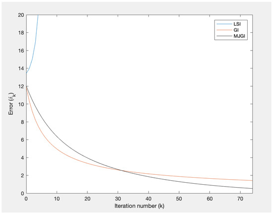
Here, E is a heptadiagonal matrix—i.e., a band matrix with bandwidth 3. Choose an initial matrix $X\left(0\right)=zeros\left(10\right),$ where $zeros\left(n\right)$ is an n-by-n matrix that contains 0 for every position. We compare Algorithm 1 with the direct method, LSI and GI algorithms. Table 1 shows the errors at the final step of iteration as well as the computation time after 75 iterations. Figure 2 illustrates that the approximated solutions via LSI diverge, while those via GI and MJGI converge. Table 1 and Figure 2 imply that our algorithm takes significantly less computational time and error than others.

Table 1. Computational time and error for Example 2.

Method	IT	CT	Error: $\mathit{\delta }\left(75\right)$
Direct	-	0.0364	-
LSI	75	0.0125	1.1296 × 105
GI	75	0.0049	1.4185
MJGI	75	0.0022	0.5251

Figure 2. Error of Example 2.

Example 3.

We consider the equation $A_{1}X{A}_2+A_{3}X{A}_4=E$ in which $A_1,A_2,A_3,A_4\mathrm{and}E$ are $100\times 100$ matrices determined by

$$\begin{array}{c}\hfill A_1=tridiag(1,1,-1),A_2=tridiag(1,2,-2),A_3=tridiag(-1,-2,3),\\ \hfill A_4=tridiag(-2,1,-1)\mathrm{and}E=heptadiag(1,2,-4,1,-2,2,-3).\end{array}$$

The initial matrix is given by $X\left(0\right)=zeros\left(100\right).$ We run LSI, GI and MJGI algorithms by using

$$\begin{array}{c}\hfill \mu =0.1,\mu ={(\Vert A_1{\Vert }^2\Vert A_2{\Vert }^2+\Vert A_3{\Vert }^2\Vert A_4{\Vert }^2)}^{-1},\mu =2{(\Vert A_1{\Vert }^2\Vert A_2{\Vert }^2+\Vert A_3{\Vert }^2\Vert A_4{\Vert }^2)}^{-1},\end{array}$$

respectively. The reported result in Table 2 and Figure 3 illustrate that the approximated solution generated from LSI diverges, while those from GI or MJGI converge. Both computational time and the error $\delta \left(100\right)$ from MJGI are less than those from GI.

Table 2. Computational time and error for Example 3.

Method	IT	CT	Error: $\mathit{\delta }\left(100\right)$
Direct	-	34.6026	-
LSI	100	0.1920	2.7572 × 104
GI	100	0.0849	4.7395
MJGI	100	0.0298	1.8844

Figure 3. Comparison of Example 3.

4.2. Numerical Simulation for Sylvester Matrix Equation

Assume that the Sylvester equation

$$\begin{array}{c}\hfill A_{1}X+X{A}_4=E\end{array}$$

(26)

has a unique solution. This condition is equivalent to that the Kronecker sum $A_4^T\oplus A_1$ is invertible, or all possible sums between eigenvalues of $A_1$ and $A_4$ are nonzero. To solve (26), the Algorithm 2 is proposed:

$$T\left(k\right):=E-A_{1}X\left(k\right)-X\left(k\right)A_4.$$

Algorithm 2: Modified Jacobi-gradient based iterative (MJGI) algorithm for Sylvester equation

Example 4.

Consider the equation $A_{1}X+X{A}_4=E,$ in which E is the same matrix as in the previous example,

$$\begin{array}{c}\hfill A_1=tridiag(2,-1,1)\in {\mathbb{R}}^{10\times 10}\mathrm{and}{A}_4=tridiag(-1,1,-2)\in {\mathbb{R}}^{10\times 10}.\end{array}$$

In this case, all eigenvalues of the iteration matrix have positive real parts, so that we can apply our algorithm. We compare our algorithm with GI, RGI, AGBI and JGI algorithms. The results after running 100 iterations are shown in Figure 4 and Table 3. According to the error and CT in Table 3 and Figure 4, our algorithm uses less computational time and has smaller errors than others.

Figure 4. Errors of Example 4.

Table 3. CTs and errors for Example 4.

Method	IT	CT	Error: $\mathit{\delta }\left(100\right)$
Direct	-	0.0118	-
GI	100	0.0051	2.5981
RGI	100	0.0061	3.4741
AGBI	100	0.0051	7.3306
JGI	100	0.0038	17.2652
MJGI	100	0.0028	0.4281

5. Conclusions and Suggestion

A modified Jacobi-gradient (MJGI) algorithm (Algorithm 1) is proposed for solving the generalized Sylvester matrix Equation (3). In order to have MJGI algorithm applicable for any sizes of matrix system and any initial matrices, the convergence factor $\mu$ must be chosen properly according to Theorem 1. In this case, the iteration matrix $I_{mn}-\mu H$ has a spectral radius less than 1. When the iteration matrix is symmetric, we determine the optimal convergent factor ${\mu }_{opt}$ which enhances the algorithm reaching the fastest rate of convergence. The asymptotic convergence rate of the algorithm is governed by the spectral radius of $I_{mn}-\mu H$. So, if the eigenvalue H is close to 1, then the algorithm converges faster in the long run. The numerical examples reveal that our algorithm is suitable for small ($2\times 2$), medium ($10\times 10$) and large ($100\times 100$) sizes of matrix systems. In addition, the MJGI algorithm performs well compared to recent gradient iterative algorithms. For future works, we may add another parameter for an updating step to make the algorithm converge faster—see [25]. Another possible way is to apply the idea in this paper to derive an iterative algorithm for nonlinear matrix equations.

References

- Shang, Y. Consensus seeking over Markovian switching networks with time-varying delays and uncertain topologies. Appl. Math. Comput. 2016, 273, 1234–1245. [Google Scholar] [CrossRef]
- Shang, Y. Average consensus in multi-agent systems with uncertain topologies and multiple time-varying delays. Linear Algebra Appl. 2014, 459, 411–429. [Google Scholar] [CrossRef]
- Golub, G.H.; Nash, S.; Van Loan, C.F. A Hessenberg-Schur method for the matrix AX + XB = C. IEEE Trans. Automat. Control. 1979, 24, 909–913. [Google Scholar] [CrossRef]
- Ding, F.; Chen, T. Hierarchical least squares identification methods for multivariable systems. IEEE Trans. Automat. Control 1997, 42, 408–411. [Google Scholar] [CrossRef]
- Benner, P.; Quintana-Orti, E.S. Solving stable generalized Lyapunov equations with the matrix sign function. Numer. Algorithms 1999, 20, 75–100. [Google Scholar] [CrossRef]
- Starke, G.; Niethammer, W. SOR for AX − XB = C. Linear Algebra Appl. 1991, 154–156, 355–375. [Google Scholar] [CrossRef]
- Jonsson, I.; Kagstrom, B. Recursive blocked algorithms for solving triangular systems—Part I: One-sided and coupled Sylvester-type matrix equations. ACM Trans. Math. Softw. 2002, 28, 392–415. [Google Scholar] [CrossRef]
- Jonsson, I.; Kagstrom, B. Recursive blocked algorithms for solving triangular systems—Part II: Two-sided and generalized Sylvester and Lyapunov matrix equations. ACM Trans. Math. Softw. 2002, 28, 416–435. [Google Scholar] [CrossRef]
- Kaabi, A.; Kerayechian, A.; Toutounian, F. A new version of successive approximations method for solving Sylvester matrix equations. Appl. Math. Comput. 2007, 186, 638–648. [Google Scholar] [CrossRef]
- Lin, Y.Q. Implicitly restarted global FOM and GMRES for nonsymmetric matrix equations and Sylvester equations. Appl. Math. Comput. 2005, 167, 1004–1025. [Google Scholar] [CrossRef]
- Kressner, D.; Sirkovic, P. Truncated low-rank methods for solving general linear matrix equations. Numer. Linear Algebra Appl. 2015, 22, 564–583. [Google Scholar] [CrossRef]
- Dehghan, M.; Shirilord, A. A generalized modified Hermitian and skew-Hermitian splitting (GMHSS) method for solving complex Sylvester matrix equation. Appl. Math. Comput. 2019, 348, 632–651. [Google Scholar] [CrossRef]
- Dehghan, M.; Shirilord, A. Solving complex Sylvester matrix equation by accelerated double-step scale splitting (ADSS) method. Eng. Comput. 2019. [Google Scholar] [CrossRef]
- Li, S.Y.; Shen, H.L.; Shao, X.H. PHSS iterative method for solving generalized Lyapunov equations. Mathematics 2019, 7, 38. [Google Scholar] [CrossRef]
- Shen, H.L.; Li, Y.R.; Shao, X.H. The four-parameter PSS method for solving the Sylvester equation. Mathematics 2019, 7, 105. [Google Scholar] [CrossRef]
- Hajarian, M. Generalized conjugate direction algorithm for solving the general coupled matrix equations over symmetric matrices. Numer. Algorithms 2016, 73, 591–609. [Google Scholar] [CrossRef]
- Hajarian, M. Extending the CGLS algorithm for least squares solutions of the generalized Sylvester-transpose matrix equations. J. Frankl. Inst. 2016, 353, 1168–1185. [Google Scholar] [CrossRef]
- Dehghan, M.; Mohammadi-Arani, R. Generalized product-type methods based on Bi-conjugate gradient (GPBiCG) for solving shifted linear systems. Comput. Appl. Math. 2017, 36, 1591–1606. [Google Scholar] [CrossRef]
- Ding, F.; Chen, T. Gradient based iterative algorithms for solving a class of matrix equations. IEEE Trans. Automat. Control 2005, 50, 1216–1221. [Google Scholar] [CrossRef]
- Niu, Q.; Wang, X.; Lu, L.-Z. A relaxed gradient based algorithm for solving Sylvester equation. Asian J. Control 2011, 13, 461–464. [Google Scholar] [CrossRef]
- Zhang, X.D.; Sheng, X.P. The relaxed gradient based iterative algorithm for the symmetric (skew symmetric) solution of the Sylvester equation AX + XB = C. Math. Probl. Eng. 2017, 2017, 1624969. [Google Scholar] [CrossRef]
- Xie, Y.J.; Ma, C.F. The accelerated gradient based iterative algorithm for solving a class of generalized Sylvester-transpose matrix equation. Appl. Math. Comput. 2012, 218, 5620–5628. [Google Scholar] [CrossRef]
- Ding, F.; Chen, T. Iterative least-squares solutions of coupled Sylvester matrix equations. Syst. Control Lett. 2005, 54, 95–107. [Google Scholar] [CrossRef]
- Fan, W.; Gu, C.; Tian, Z. Jacobi-gradient iterative algorithms for Sylvester matrix equations. In Proceedings of the 14th Conference of the International Linear Algebra Society, Shanghai University, Shanghai, China, 16–20 July 2007. [Google Scholar]
- Tian, Z.; Tian, M.; Gu, C.; Hao, X. An accelerated Jacobi-gradient based iterative algorithm for solving Sylvester matrix equations. Filomat 2017, 31, 2381–2390. [Google Scholar] [CrossRef]
- Ding, F.; Liu, P.X.; Chen, T. Iterative solutions of the generalized Sylvester matrix equations by using the hierarchical identification principle. Appl. Math. Comput. 2008, 197, 41–50. [Google Scholar] [CrossRef]
- Horn, R.A.; Johnson, C.R. Topics in Matrix Analysis; Cambridge University Press: New York, NY, USA, 1991. [Google Scholar]
Publisher’s Note: MDPI stays neutral with regard to jurisdictional claims in published maps and institutional affiliations. |
© 2020 by the authors. Licensee MDPI, Basel, Switzerland. This article is an open access article distributed under the terms and conditions of the Creative Commons Attribution (CC BY) license (http://creativecommons.org/licenses/by/4.0/).