Despeckling Algorithm for Removing Speckle Noise from Ultrasound Images

Abstract

Ultrasound (US) imaging can examine human bodies of various ages; however, in the process of obtaining a US image, speckle noise is generated. The speckle noise inhibits physicians from accurately examining lesions; thus, a speckle noise removal method is essential technology. To enhance speckle noise elimination, we propose a novel algorithm using the characteristics of speckle noise and filtering methods based on speckle reducing anisotropic diffusion (SRAD) filtering, discrete wavelet transform (DWT) using symmetry characteristics, weighted guided image filtering (WGIF), and gradient domain guided image filtering (GDGIF). The SRAD filter is exploited as a preprocessing filter because it can be directly applied to a medical US image containing speckle noise without a log-compression. The wavelet domain has the advantage of suppressing the additive noise. Therefore, a homomorphic transformation is utilized to convert the multiplicative noise into additive noise. After two-level DWT decomposition is applied, to suppress the residual noise of an SRAD filtered image, GDGIF and WGIF are exploited to reduce noise from seven high-frequency sub-band images and one low-frequency sub-band image, respectively. Finally, a noise-free image is attained through inverse DWT and an exponential transform. The proposed algorithm exhibits excellent speckle noise elimination and edge conservation as compared with conventional denoising methods.

1. Introduction

Ultrasound (US) imaging devices have been exploited to examine human bodies of various ages, from young to old people; in fact, US imaging is one of the most widely used imaging technologies in the medical diagnosis field. US imaging devices can be inexpensive, protected from radiation, and portable compared with other medical imaging devices such as X-ray imaging, computer tomography, magnetic resonance imaging, and positron emission tomography [1,2]. Another advantage is that it can produce a real-time image. Based on these merits, US imaging devices are widely utilized to diagnose lesions in muscles, joints, blood vessels, and internal organs. US imaging is also used to examine fetuses of pregnant women, which can be viewed safely and in real time.

An inherent characteristic of US images is speckle noise [3]. Speckle noise in medical US images is caused by backscattered echo signals [4]. Speckle noise has the characteristics of multiplicative noise and Rayleigh distribution, degrading the image resolution and contrast because of the granular pattern that appears in the images [5]. Speckle noise in medical US images prevents physicians from performing accurate lesion diagnosis because they hinder the extraction, analysis, and recognition of lesion features. To gain a reliable lesion diagnosis and analysis through US imaging, a speckle noise suppression algorithm is an essential preprocessing technique.

In the past few years, numerous algorithms have been developed to eliminate speckle noise from US and digital images. This study presents four categories of speckle noise reduction methods: single filter, nonlocal means (NLM)-based algorithm, despeckling of sub-band images in the transform domain, and speckle noise suppression in the transform domain. Among the single filter methods that made use of eliminating speckle noise from ultrasonography images are the Lee [6], Kuan [7], Frost [8], modified Lee filter [9], modified Frost filter [9], and anisotropic diffusion filtering [10,11] methods. Since these filtering methods tend to result in a smoothing phenomenon at the edges, these techniques are not optimal for removing speckle noise. They also turn up a loss of edge information, such as texture patterns and other important details.

Despeckling algorithms combining various techniques have been proposed to overcome the problems of single filtering methods. To suppress speckle noise, an optimized Bayesian-based nonlocal mean (OBNLM) method was proposed by Coupe et al. [12]. The OBNLM technique was employed through the block-wise nonlocal means (NLM) approach. Then, the Pearson distance measure was utilized in the OBNLM method to calculate the similarity between two patches in the image to suppress speckle noise. Yang et al. [13] developed an algorithm using local statistics based on the NLM filter to reduce speckle noise. Radlak and Smolka [14] proposed a method based on an adaptive NLM filter. Sudeep et al. [15] put forward a novel algorithm by considering different parameters of speckle noise statistics based on the maximum likelihood estimation method. Although NLM-based algorithms have been developed, these methods tend to generate over-smoothed images, with speckle noise remaining near the edge regions. Tounsi et al. [16] suggested a method of eliminating speckle noise by exploiting a variant NLM technique. In their study, NLM-based adaptive patches and a few reprojection (central reprojection, uniform average of estimators reprojection, and minimizing variance-reprojection etc.) utilizing the NLM filter were primarily used; however, their method showed a low speckle noise rejection ability in the non-homogeneous areas. Furthermore, to eliminate speckle noise in digital images, a despeckling technique using the NLM filter and adaptive mask-based filtering techniques, similar to the NLM method, was proposed by Tounsi et al. [17]. Although this algorithm conserved the outstanding feature information, it exhibited low speckle noise rejection ability in the flat areas. Santos et al. [18] proposed a despeckling method based on block-matching collaborative filtering (BM3D) and novel stochastic distance techniques. Although this algorithm has superb feature information conservation ability, speckle noise still remains in the homogeneous areas of US images.

To take advantage of the statistical characteristics of sub-band images in the transform domain, despeckling algorithms utilize each distribution of sub-band images based on prior knowledge. Portilla et al. [19] proposed a speckle noise suppression algorithm using Bayesian least squares with a Gaussian mixture model. In [20], an algorithm exploiting the Gaussian mixture model to suit coefficients for the distribution of sub-band images in the transform domain was proposed. After these experiments, a generalized Gaussian distribution [21] made use of suiting a distribution of the data. To adapt to various statistical model conditions, probability density functions such as the normal inverse Gaussian [22], Laplace distribution [23], and Cauchy Rayleigh distribution [24] have been utilized.

In a few experiments, algorithms employing a transform domain have been developed to eliminate speckle noise from images. Zada et al. [25] proposed a speckle noise reduction algorithm based on the monogenic wavelet transform in digital images. This algorithm showed an outstanding speckle noise elimination ability but exhibited artifacts in the non-edge areas. Furthermore, Trusiak et al. [26] employed a modified fast and adaptive bi-dimensional empirical mode decomposition and the Hilbert spiral transform for reducing speckle noise. Although this method showed a remarkable speckle noise elimination ability, there was a loss of edge information in some of the feature regions. In [27], a despeckling method was proposed using the intra-scale correlation in the wavelet domain. Fathi and Naghsh [28] developed a despeckling technique utilizing a threshold method in the transform domain to suppress speckle noise. In wavelet transform, a despeckling algorithm was suggested using the Bayesian minimum mean square error (MMSE) [29]. Baselice et al. [30] provided a suggestion to overcome a limitation of the Wiener filtering method. In [30], various techniques such as the enhanced Wiener filter, fast Fourier transform (FFT), and Markov random field (MRF) were adopted. The enhanced Wiener filter tunes the mask size to obtain noise reduction and detail conservation. The speckle noise removal methodology uses the MRF technique in the FFT domain to reduce the computational burden of the algorithm. The algorithm of Baselice et al. achieved good filtering performance but was accompanied by a loss of edge information. However, as mentioned above, most algorithms for speckle noise reduction in medical US images appear to have low speckle noise elimination and feature preservation abilities. Therefore, to realize an excellent ability of speckle noise removal and edge information conservation, we propose an algorithm utilizing a speckle reducing anisotropic diffusion (SRAD) filter [31], discrete wavelet transform (DWT) employing symmetry characteristics, gradient domain guided image filtering (GDGIF) [32], and weighted guided image filtering (WGIF) [33]. Under the condition of multiplicative noise, the SRAD filtering technique can be directly employed to suppress speckle noise because it can be directly applied to a medical US image including speckle noise without a log-compression. The wavelet domain has the advantage of eliminating additive noise (additive white Gaussian noise) [34]. Therefore, we used a homomorphic transformation to convert the multiplicative noise into additive noise in the SRAD resulting image. A two-level DWT decomposition, which employs the symmetry characteristics, produces seven high-frequency sub-band images and a low-frequency sub-band image from the SRAD resultant image to retain each of the wavelet coefficients and remove the noise. Finally, a noise-free image taking advantage of DWT reconstruction and exponential transformation is obtained.

This paper is organized as follows. In Section 2, we propose a new method for eliminating speckle noise and conserving edges based on SRAD, DWT, GDGIF, and WGIF. Experimental results of the conventional methods and proposed algorithm are analyzed in Section 3. Finally, the conclusion is presented in Section 4.

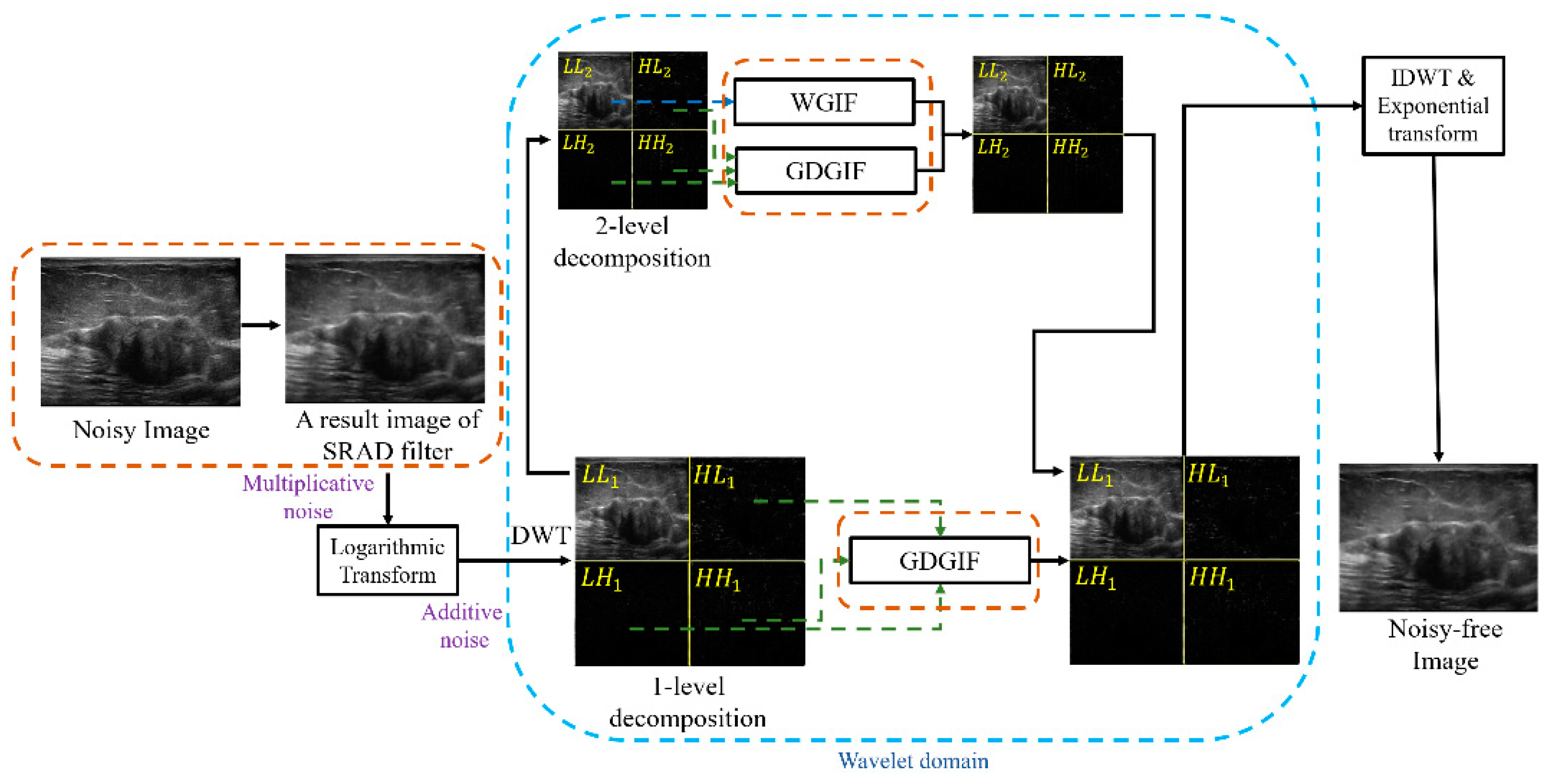
2. Proposed Algorithm

A flowchart of the proposed method is shown in Figure 1. The SRAD filtering method has a superb speckle noise reduction and detail information conservation performance because an instantaneous coefficient of variation (ICOV) in the SRAD filter can classify feature areas in speckled imagery [31]. Therefore, the SRAD filter was utilized as a preprocessing filter in the proposed algorithm. Understanding the statistical model for suppressing noise in the wavelet domain can lead to improvement in speckle noise removal from US images.

The additive noise, which possesses the characteristics of additive white Gaussian noise, can be reduced in the wavelet domain [34]; thus, we utilize a homomorphic transformation to convert the multiplicative noise into additive noise in the resulting image of the SRAD filter. The two-level wavelet decomposition can convert a parent image (SRAD resulting image) into seven high-frequency sub-band images and a low-frequency sub-band image. The wavelet coefficients in the high-frequency sub-band images are conserved, whereas the additive noise in the high-frequency sub-band images are eliminated for the GDGIF. Meanwhile, as the low-frequency sub-band image in the wavelet domain includes large speckle noise [35], the WGIF is exploited to suppress the speckle noise in the low-frequency sub-band image while conserving the edges. Finally, a despeckled image is gained using wavelet reconstruction and exponential transformation.

2.1. Speckle Reducing Anisotropic Diffusion Filter

A partial differential equation was exploited for the SRAD filter to eliminate the speckle noise in medical US images (Equation (1)).

$$\{\begin{array}{c}\frac{\partial I\left(x,y;t\right)}{\partial t}=div\left[c\left(q\right)\nabla I\left(x,y;t\right)\right]\\ I\left(x, y;0\right)=I_0\left(x, y\right),\hspace{1em}{\left(\frac{\partial I\left(x,y;t\right)}{\partial \overrightarrow{n}}\right)|}_{\partial \mathsf{\Omega }}=0\end{array}$$

(1)

where $I_0\left(x, y\right)$ and $I\left(x,y;t\right)$ are the initial and output images, respectively, $\nabla$ denotes the gradient operator, $div$ is a divergence operator, $\partial \mathsf{\Omega }$ is the boundary of $\mathsf{\Omega }$, and $\overrightarrow{n}$ is the outer normal of $\partial \mathsf{\Omega }$. In Equation (1), the diffusion coefficient $c\left(q\right)$ determines which diffusion process is exploited to eliminate speckle noise. The diffusion coefficient $c\left(q\right)$ is calculated as follows:

$$c\left(q\right)=\frac{1}{\frac{1+\left[q^2\left(x,y;t\right)-q_0^2\left(t\right)\right]}{\left[q_0^2\left(t\right)\left(1+q_0^2\left(t\right)\right)\right]}}$$

(2)

where $q\left(x,y;t\right)$ and $q_0\left(t\right)$ are the instantaneous coefficient of variation (ICOV) and speckle scale function, respectively. The ICOV is utilized as an edge detector in US images containing speckle noise (Equation (3)).

$$q\left(x,y;t\right)=\sqrt{\frac{\left(\frac{1}{2}\right){\left(\frac{\left|\nabla I\right|}{I}\right)}^2-\left(\frac{1}{4^2}\right){\left(\frac{{\nabla }^{2}I}{I}\right)}^2}{{\left[1+\left(\frac{1}{4}\right)\left(\frac{{\nabla }^{2}I}{I}\right)\right]}^2}}$$

(3)

where ${\nabla }^2$ is the Laplacian operator. The ICOV displays high values at the edge areas and low values in the flat regions. The speckle scale function $q_0\left(t\right)$ plays a role as the diffusion threshold in Equation (2). This function is given by

$$q_0\left(t\right)=\frac{\sqrt{var\left[z\left(t\right)\right]}}{\overline{z\left(t\right)}}$$

(4)

where $\overline{z\left(t\right)}$ and $var\left[z\left(t\right)\right]$ are the mean and variance, respectively, over a flat area at $t$. The diffusion threshold can be adjusted according to regions in the image whether to promote or inhibit smoothing. Therefore, this function can eliminate speckle noise in flat areas and conserve the edge information. According to the functions mentioned above, the SRAD filtering technique can be directly applied to medical US images that contain speckle noise to remove the speckle noise and preserve the features. We make use of the SRAD filter as a pretreatment filtering method.

2.2. A Model of Speckle Noise

The SRAD filtered resulting image consists of two parts: the useful signal and the noise. The noise consists of multiplicative noise and additive noise. The multiplicative noise is related to the principle of medical US imaging [35,36], whereas additive noise is the noise generated by the sensor [10]. The speckle noise model of the SRAD resulting image can be written as:

$$F\left(x,y\right)=O\left(x,y\right)\times W\left(x,y\right)+A\left(x,y\right)$$

(5)

where $O\left(x,y\right)$, $W\left(x,y\right)$, and $A\left(x,y\right)$ are the original signal, multiplicative noise, and additive noise, respectively. In Equation (5), the additive noise $A\left(x,y\right)$ is omitted because the effect of the additive noise $A\left(x,y\right)$, compared with that of the multiplicative noise $W\left(x,y\right)$, is considerably small. Thus, Equation (5) can be represented by Equation (6).

$$F\left(x,y\right)=O\left(x,y\right)\times W\left(x,y\right)$$

(6)

Here, multiplicative noise $W\left(x,y\right)$ obeys the Rayleigh distribution [34]. In the research field of noise reduction, DWT using symmetry characteristics is typically utilized to eliminate additive noise. Therefore, a model of multiplicative noise is converted into a model of additive noise exploiting a homomorphic transformation (Equation (7)).

$$\log \left(F\left(x,y\right)\right)=\log \left(O\left(x,y\right)\right)+\log \left(W\left(x,y\right)\right)$$

(7)

where $\log \left(F\left(x,y\right)\right)$ is a medical US image, and $\log \left(W\left(x,y\right)\right)$ follows the characteristics of additive Gaussian white noise [34].

2.3. Discrete Wavelet Transform

To suppress the additive noise in the high-frequency sub-band images and low-frequency sub-band image of the wavelet domain, at each step, we can acquire four different sub-band images with different orientations and components depending on scale and translation parameters. DWT based on symmetry characteristics decomposes the signal into a set of basis functions to obtain each sub-band image (Equation (8)). As the scale and translation parameters can be applied in the wavelet decomposition on the DWT, each sub-band image is obtained exploiting this process. That is, wavelet ${\Psi }_{j,k}\left(t\right)$ is a set of functions attained by scaling in or out and translating the mother wavelet $\Psi \left(t\right)$.

$${\Psi }_{j,k}\left(t\right)=2^{-\frac{j}{2}} \Psi \left(2^{-j}t-k\right)$$

(8)

where $\Psi \left(t\right)$ is the mother wavelet, $j$ is a component for adjusting the scale parameter, and $k$ is a translation parameter that represents a constituent frequency moving along the time axis. The scale parameter can distinguish the local characteristics of a signal at a variety of scales, whereas the translation parameter can cover the entire region. The signal $f\left(t\right)$ is represented by a linear combination of wavelet coefficients $c_{j,k}$ and wavelet ${\Psi }_{j,k}\left(t\right)$ (Equation (9)).

$$f\left(t\right)={\displaystyle \sum }_{j,k}{c}_{j,k}{\Psi }_{j,k}\left(t\right)$$

(9)

Figure 2 displays the one-level wavelet decomposition process for two-dimensional (2D) images. In the one-level wavelet decomposition, a low-pass and a high-pass filter are applied to a 2D image in the horizontal direction. The result of applying the pass filter in the horizontal direction is to reduce the size to a half through down sampling. By applying the same process to the vertical direction, four sub-band images ($L{L}_1,L{H}_1,H{L}_1,H{H}_1)$ are obtained. $L{H}_1,H{L}_1,\mathrm{and}H{H}_1$ are high-frequency sub-band images in the horizontal, vertical, and diagonal directions, respectively, whereas $L{L}_1$ is a low-frequency sub-band image. $L{L}_1$ is used as the input image of the next wavelet decomposition process to be divided into high-frequency sub-band images ($L{H}_2,H{L}_2,H{H}_2$) and a low-frequency sub-band image ($L{L}_2$). That is, three high-frequency sub-band images ($L{H}_1,H{L}_1,H{H}_1$) and a low-frequency sub-band image ($L{L}_1$) are acquired utilizing a one-level wavelet decomposition process. In two-level wavelet decomposition, the low-frequency sub-band image is divided into three high-frequency sub-band images ($L{H}_2,H{L}_2,H{H}_2$) and a low-frequency sub-band image ($L{L}_2$).

In this study, wavelet decomposition was performed up to level two, and among the types of bior, coif, db, dmey, sym, haar, and rbio, sym was used (Figure 3).

2.4. Gradient Domain Guided Image Filtering in the High-Frequency Sub-Band Images

In the wavelet domain, many studies have used threshold methods based on hard [37], soft [36], and Bayes [37,38] thresholds to eliminate the noise in high-frequency sub-band images [35,39,40,41]. The ability of the GDGIF based on first-order edge-aware to provide detailed information was verified in [32] through the method of single-image detail enhancement; thus, we make use of the GDGIF to eliminate noise and conserve edges in the high-frequency sub-band images.

The most important assumption in the guided image filtering (GIF) process is a local linear model between guidance $G$ and filtering output $q$. The cost function of the GIF is defined as:

$$q_i=a_h{G}_i+b_h,\hspace{1em}\forall i\in {\omega }_h$$

(10)

where $(a_h, b_h)$ are linear coefficients in square window ${\omega }_h$, which has mask size $h$. To determine the linear coefficients $(a_h, b_h)$, from the filtering input, noise components were subtracted to acquire filtering output $q$ (Equation (11)).

$$q_i=p_i-n_i$$

(11)

A cost function of GDGIF is defined as

$$E(a_h, b_h)={\displaystyle \sum }_{i\in {\omega }_h}[{\left(a_h{G}_i+b_h-p_i\right)}^2+\frac{\lambda }{{\tau }_G\left(h\right)}{\left(a_h-{\vartheta }_h\right)}^2]$$

(12)

where ${\tau }_G\left(h\right)$ is an edge-aware weight based on first-order of the GDGIF. The first-order edge-aware weight of the GDGIF is as follows:

$${\tau }_G\left(h\right)=\frac{1}{N}{\displaystyle \sum }_{h=1}^N\frac{\aleph \left(h^{\prime }\right)+\epsilon }{\aleph \left(h\right)+\epsilon }$$

(13)

where ${\tau }_G\left(h\right)$ makes use of the local variance of $3\times 3$ masks and $\left(2h+1\right)\times \left(2h+1\right)$ windows. The size of $\aleph \left(h^{\prime }\right)$ is ${\sigma }_{G,1}\left(h^{\prime }\right){\sigma }_{G,h}\left(h^{\prime }\right)$. The weight of the GDGIF ${\tau }_G\left(h\right)$ plays an analogous role to the weight of the WGIF [33]. Parameter ${\vartheta }_h$ is represented as follows.

$${\vartheta }_h=1-\frac{1}{1+e^{\eta \left(\chi \left(h^{\prime }\right)-{\mu }_{\chi ,\infty }\right)}}$$

(14)

where ${\mu }_{\chi ,\infty }$ is the mean value of all $\chi \left(p\right)$ and $\eta$ is calculated as $\frac{4}{\left({\mu }_{\chi ,\infty }-\min \left(\chi \left(p\right)\right)\right)}$. When ${\vartheta }_h$ is located at the edge areas, the value of ${\vartheta }_h$ approximates 1. In the homogeneous regions, the value of ${\vartheta }_h$ approaches 0.

The optimized values of $a_{h_1}$ and $b_{h_1}$ are expressed as follows.

$$a_{h_1}=\frac{{\mu }_{G\ast q}\left(h\right)-{\mu }_G\left(h\right){\mu }_q\left(h\right)+\frac{\lambda }{{\tau }_G\left(h\right)}{\vartheta }_h}{{\sigma }_G^2+\frac{\lambda }{{\tau }_G\left(h\right)}}$$

(15)

$$b_{h_1}={\mu }_q\left(h\right)-a_h{\mu }_G\left(h\right)$$

(16)

The final value of $p_i^1$ is expressed as follows.

$$p_i^1={\overline{a}}_{h_1}{G}_i+{\overline{b}}_{h_1}$$

(17)

where ${\overline{a}}_{h_1}$ and ${\overline{b}}_{h_1}$ are the mean values of $a_{h_1}$ and $b_{h_1}$ in the window, respectively.

2.5. Weighted Guided Image Filtering in the Low-Frequency Sub-Band Image

In [12], it is confirmed that noise is present in a low-frequency sub-band image in the wavelet domain. Zhang and Gunturk take advantage of a bilateral filter (BF) [42] to eliminate the noise from the low-frequency sub-band image. Since BF uses the Gaussian-weighted average, the BF exhibits artifacts around the edge regions [43]. To overcome this problem, Zhang et al. [35] suppressed noise without artifacts by applying a GIF [43] to the low-frequency sub-band image. Although the GIF outperforms the BF, the value of the regularization parameter in the GIF is fixed [33]. It is impossible to avoid halo artifacts when the GIF is exploited because the GIF serves to smooth edge areas. Therefore, we make use of a WGIF [33] utilizing zeroth-order edge-aware weight to remove the additive noise and conserve feature information.

From Equation (10) of the GIF, the values of $u_h$ and $v_h$ are obtained by minimizing cost function $E$. The cost function of the linear coefficients $E(u_h, v_h)$ is as follows:

$$E(u_h, v_h)={\displaystyle \sum }_{i\in {\omega }_h}[{\left(u_h{G}_i+v_h-p_i\right)}^2+\frac{\lambda }{{\gamma }_G\left(h\right)}{c}_h^2]$$

(18)

where $\lambda$ is a regularization parameter. From Equation (18), ${\gamma }_G\left(h\right)$ is an edge-aware weight exploiting zeroth-order of the WGIF. The edge-aware weight of the WGIF is defined as

$${\gamma }_G\left(h\right)=\frac{1}{N}{\displaystyle \sum }_{h=1}^N\frac{{\sigma }_{G,1}^2\left(h^{\prime }\right)+\epsilon }{{\sigma }_{G,1}^2\left(h\right)+\epsilon }$$

(19)

where ${\sigma }_{G,1}^2\left(h^{\prime }\right)$ is the variance of the guidance image in the window, $\epsilon$ is a small constant selected as ${\left(0.001\times L\right)}^2$, $L$ is the dynamic range of the input image, and the weight ${\gamma }_G\left(h\right)$ compares pixel with the entire guidance image [33]. The value of ${\gamma }_G\left(h\right)$ in the edge areas is larger than 1 but smaller than 1 in the homogeneous regions.

The optimal values of $\left(u_{h_2}, v_{h_2}\right)$ are calculated as

$$u_{h_2}=\frac{{\mu }_{G\ast q}\left(h\right)-{\mu }_G\left(h\right){\mu }_q\left(h\right)}{{\sigma }_G^2+\frac{\lambda }{{\gamma }_G\left(h\right)}}$$

(20)

$$v_{h_2}={\mu }_q\left(h\right)-u_h{\mu }_G\left(h\right)$$

(21)

where $\ast$ is the element-by-element product of two matrices, and ${\mu }_{G\ast q}\left(h\right)$, ${\mu }_G\left(h\right)$, and ${\mu }_q\left(h\right)$ are the mean values $G\ast q$, $G$, and $q$, respectively.

The final value of $p_{ii}^2$ is computed by

$$p_{ii}^2={\overline{u}}_{h_2}{G}_i+{\overline{v}}_{h_2}$$

(22)

where ${\overline{u}}_{h_2}$ and ${\overline{v}}_{h_2}$ are the mean values of $u_{h_2}$ and $v_{h_2}$ in the window.

2.6. Evaluation Metrics

In this experiment, three evaluation metrics are utilized to assess the abilities of speckle noise elimination and edge conservation in standard and real US images. The peak signal-to-noise ratio (PSNR) and structural similarity (SSIM) are exploited to measure the performances of speckle noise suppression and feature conservation in standard images [44]. To measure the ability of speckle noise suppression in the flat areas of real US images, we use an equivalent number of looks (ENL) metric [44]. A speckle suppression and mean preservation index (SMPI) is utilized to evaluate the despeckling performance [18]. The PSNR is calculated as

$$PSNR=20{\log }_{10}\left(\frac{255}{\sqrt{MSE}}\right).$$

(23)

where the mean square error (MSE) is defined by

$$MSE=\frac{1}{MN}{\displaystyle \sum }_{x=0}^{M-1}{\displaystyle \sum }_{y=0}^{N-1}{\left\{f\left(M, N\right)-g\left(M, N\right)\right\}}^2$$

(24)

where $M$ and $N$ are the number of rows and columns, respectively, $f$ is the original image, and $g$ is the result image obtained from the noisy image, applying the filtering method. The MSE represents the similarity between the original image and resulting image. A low MSE value denotes that the resulting image is close to the original image. The PSNR is utilized to evaluate the performance of speckle noise elimination. A high PSNR value indicates excellent speckle noise suppression ability. The SSIM value measures the similarity between the original image and resulting image. The SSIM is defined as:

$$SSIM\left(x, y\right)=\frac{\left(2{\mu }_x{\mu }_y+c_1\right)\left(2co{v}_{xy}+c_2\right)}{\left({\mu }_x^2+{\mu }_y^2+c_1\right)\left({\sigma }_x^2+{\sigma }_y^2+c_2\right)}$$

(25)

where ${\mu }_x$, ${\mu }_y$, ${\sigma }_x^2$, and ${\sigma }_y^2$ are the means of the original image and resulting image and variances of the original image and resulting image, respectively, $co{v}_{xy}$ represents the covariance of $x$ and $y$, and $c_1$ and $c_2$ are two positive values used to prevent the denominator from going to zero. The value range of SSIM is from 0 to 1, and the higher the SSIM value, the more optimal the result. To assess the speckle noise suppression in the homogeneous regions, ENL is used and is computed as follows,

$$ENL=\frac{{\mu }_{ROI}^2}{{\sigma }_{ROI}^2}.$$

(26)

Here, ${\mu }_{ROI}^2$ and ${\sigma }_{ROI}^2$ denote the mean and standard deviation in the region of interest (ROI) of the US images, respectively. A high value represents excellent speckle noise suppression ability in the flat areas. A speckle suppression index (SSI) is not reliable, as the mean value of SSI is overestimated in the filtered image. Therefore, the SMPI is used to accurately measure the despeckling performance. An equation of SMPI is represented as

$$SMPI=(Q+|mean(E\left[n\right]-E\left[g\right]|)\left(\frac{\sqrt{var\left[g\right]}}{\sqrt{var\left[n\right]}}\right).$$

(27)

Here,

$$Q=\left(\frac{\max \left(E\left[g\right]-\min \left(E\left[g\right]\right)\right)}{E\left[n\right]}\right)$$

(28)

where $E$ [] and $var[]$ denote the expected and variance values, respectively. $n$ indicates the noise image. A lower value of SMPI represents a higher despeckling ability [45].

3. Experimental Results

3.1. Experimental Environments of Standard Images and US Images

To appraise the performance of speckle noise elimination with the conventional methods and proposed algorithm, six standard images, namely, Airplane (512 $\times$ 512), Boat (512 $\times$ 512), Cameraman (256 $\times$ 256), Man (1024 $\times$ 1024), Lena (512 $\times$ 512), and Peppers (512 $\times$ 512) were selected, and five US images (US images of malignant breast lesions (300 $\times$ 225) [46] and an US phantom image (257 $\times$ 257) were selected (Figure 4 and Figure 5). Real US images of malignant breast lesions were obtained using a Hitachi Ultrasound System [46]. To assess the performance of speckle noise removal, we added speckle noise with variance ($\sigma =0.04)$ to the standard images, as shown in Figure 4.

Figure 5 designates two ROIs in the US images to measure the speckle noise suppression ability in the homogeneous areas. The speckle noise elimination and feature preservation performances of the conventional methods (Gaussian [31], Lee [6], Frost [8], anisotropic diffusion filter with memory based on speckle statistics (ADMSS) [47], SRAD [31], weighted least squares (WLS) [48], GIF [43], Bitonic [49], SRAD-Bayes algorithm [44], and synthetic aperture radar block matching 3-D (SAR-BM3D) [50]), and the proposed algorithm were compared. All experiments related to image processing were conducted using MATLAB R2018b (MathWorks, Natick, MA) on an Intel(R) Core(TM) i5-8500 CPU @ 3.0 GHz, 16 GB RAM, and 64-bit operating system.

Table 1. Optimal parameters for the proposed algorithm in the standard images. GDGIF: gradient domain guided image filtering, SRAD: speckle reducing anisotropic diffusion, WGIF: weighted guided image filtering.

	SRAD	GDGIF	WGIF
Airplane	Time step = 0.01 Exponential rate = 1 Number of iterations = 130	Mask size = 9 $\times$ 9 Regularization parameter = 0.01	Mask size = 9 $\times$ 9 Regularization parameter = 1 × 10−6
Boat	Time step = 0.01 Exponential rate = 1 Number of iterations = 100	Mask size = 9 $\times$ 9 Regularization parameter = 0.01	Mask size = 9 $\times$ 9 Regularization parameter = 1 × 10−6
Cameraman	Time step = 0.01 Exponential rate = 1 Number of iterations = 180	Mask size = 9 $\times$ 9 Regularization parameter = 0.01	Mask size = 9 $\times$ 9 Regularization parameter = 1 × 10−6
Man	Time step = 0.01 Exponential rate = 1 Number of iterations = 120	Mask size = 9 $\times$ 9 Regularization parameter = 0.01	Mask size = 9 $\times$ 9 Regularization parameter = 1 × 10−6
Lena	Time step = 0.01 Exponential rate = 1 Number of iterations = 150	Mask size = 9 $\times$ 9 Regularization parameter = 0.01	Mask size = 9 $\times$ 9 Regularization parameter = 1 × 10−6
Peppers	Time step = 0.01 Exponential rate = 1 Number of iterations = 150	Mask size = 9 $\times$ 9 Regularization parameter = 0.01	Mask size = 9 $\times$ 9 Regularization parameter = 1 × 10−6

,

Table 2. Optimal parameters for the proposed algorithm in the US images.

	SRAD	GDGIF	WGIF
US image 1	Time step = 0.01 Exponential rate = 1 Number of iterations = 130	Mask size = 9 $\times$ 9 Regularization parameter = 0.01	Mask size = 9 $\times$ 9 Regularization parameter = 1 × 10−6
US image 2	Time step = 0.01 Exponential rate = 1 Number of iterations = 80	Mask size = 9 $\times$ 9 Regularization parameter = 0.01	Mask size = 9 $\times$ 9 Regularization parameter = 1 × 10−6
US image 3	Time step = 0.01 Exponential rate = 1 Number of iterations = 140	Mask size = 9 $\times$ 9 Regularization parameter = 0.01	Mask size = 9 $\times$ 9 Regularization parameter = 1 × 10−6
US image 4	Time step = 0.01 Exponential rate = 1 Number of iterations = 90	Mask size = 9 $\times$ 9 Regularization parameter = 0.01	Mask size = 9 $\times$ 9 Regularization parameter = 1 × 10−6
US image 5	Time step = 0.01 Exponential rate = 1 Number of iterations = 60	Mask size = 9 $\times$ 9 Regularization parameter = 0.01	Mask size = 9 $\times$ 9 Regularization parameter = 1 × 10−6
US image 6	Time step = 0.01 Exponential rate = 1 Number of iterations = 100	Mask size = 9 $\times$ 9 Regularization parameter = 0.01	Mask size = 9 $\times$ 9 Regularization parameter = 1 × 10−6

and

Table 3. Optimal parameters for the conventional methods in the standard and US images. ADMSS: anisotropic diffusion filter with memory based on speckle statistics, BM3D: block-matching collaborative filtering, WLS: weighted least squares.

	Six Standard Images	Six US Images
Guided	Mask size = 3 $\times$ 3 Regularization parameter = 0.001	Mask size = 3 $\times$ 3 Regularization parameter = 0.001
Lee	Mask size = 3 $\times$ 3	Mask size = 3 $\times$ 3
Frost	Mask size = 3 $\times$ 3	Mask size = 3 $\times$ 3
Gaussian	Mask size = 5 $\times$ 5 ${\sigma }^2=2$	Mask size = 5 $\times$ 5 ${\sigma }^2=2$
Bitonic	Mask size = 3 $\times$ 3	Mask size = 3 $\times$ 3
WLS	$\mathsf{\lambda }$ = 0.5	$\mathsf{\lambda }$ = 0.5
ADMSS	${\Delta }_t$ = 0.5, $\sigma =\mathsf{\rho }$ = 0.1, $n_{iter}$ = 15	${\Delta }_t$ = 0.5, $\sigma =\mathsf{\rho }$ = 0.1, $n_{iter}$ = 15
SAR-BM3D	Number of rows/cols of block = 9, Maximum size of the 3rd dimension of a stack = 16, Diameter of search area = 39, Dimension of step = 3, Parameter of the 2D Kaiser window = 2, Transform: undecimated wavelet transform (UDWT) = daub4	Number of rows/cols of block = 9, Maximum size of the 3rd dimension of a stack = 16, Diameter of search area = 39, Dimension of step = 3, Parameter of the 2D Kaiser window = 2, Transform: UDWT = daub4

indicate the optimal parameters of the existing denoising techniques and the proposed algorithm for standard and US images. In the standard and US images, the optimal parameter of the SRAD filtering method in the SRAD-Bayes algorithm [44] and the SRAD filtering technique are the same as the parameters of the SRAD filter in Table 1 and Table 2. The best parameters for the conventional methods are listed in Table 3.

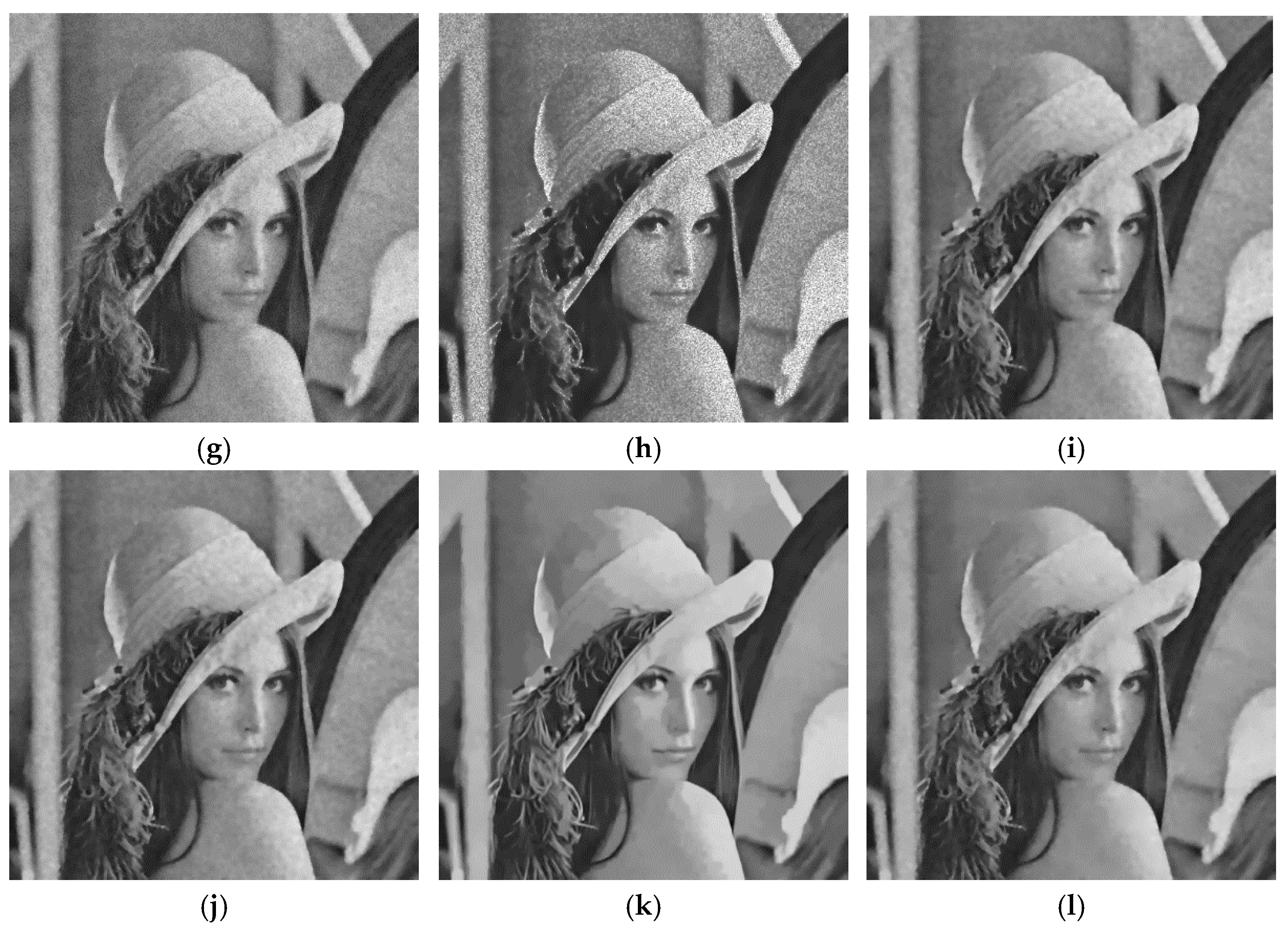
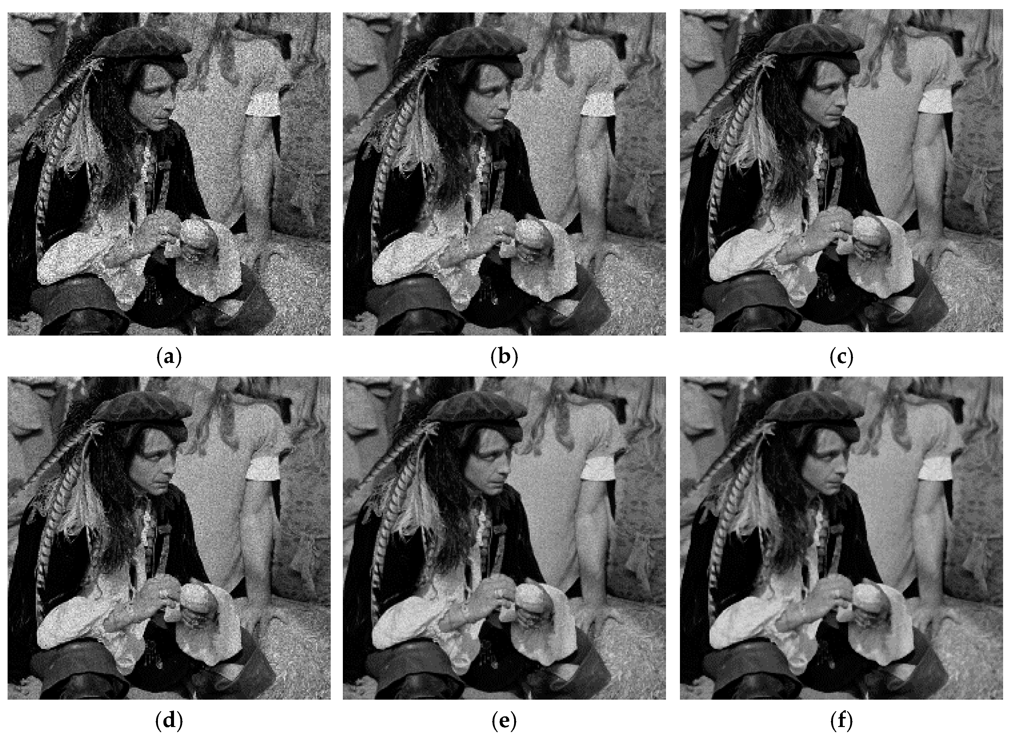
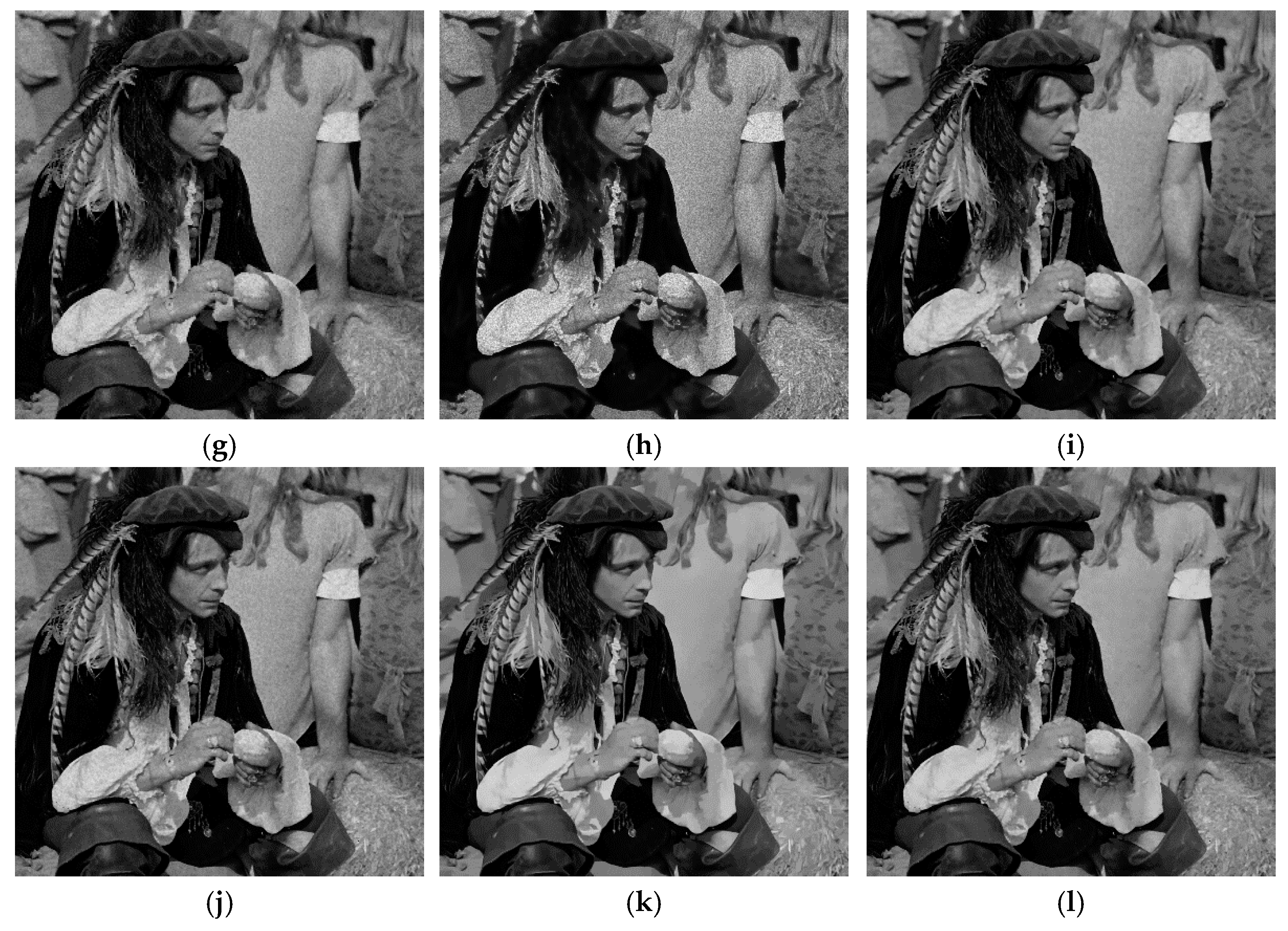
3.1.1. Experiments on Standard Images

The PSNR and SSIM values of the conventional noise elimination techniques and proposed algorithm are computed for comparison (

Table 4. Comparison of peak signal-to-noise ratio (PSNR) values of the conventional methods and the proposed algorithm.

	Airplane	Boat	Cameraman	Man	Lena	Peppers
Noisy	16.5259	18.4571	18.6368	20.6950	18.8416	18.5572
GIF	19.1425	18.4571	24.3955	24.1908	22.3112	20.7189
Lee	23.7811	24.9209	23.0668	27.4333	25.8835	25.5090
Frost	22.0637	23.3875	22.3281	25.5420	24.2903	23.3401
Gaussian	25.1845	25.3322	22.5199	27.5073	27.4245	27.6756
Bitonic	26.1829	26.4246	24.3955	26.7991	28.5419	28.2365
WLS	25.6469	26.3535	25.9689	28.4255	28.0356	28.7923
ADMSS	23.4343	20.1359	17.5853	23.6321	21.8759	18.2932
SRAD	26.5703	27.4141	26.3295	29.2499	29.6899	30.4284
SRAD-Bayes	27.0275	27.4154	26.4097	29.5813	29.6899	30.4284
SAR-BM3D	32.9288	27.2015	26.3454	28.8885	29.9061	29.7615
Proposed	27.4755	27.7553	26.4681	29.6691	29.9126	30.5983

and

Table 5. Comparison of structural similarity (SSIM) values of the conventional methods and the proposed algorithm.

	Airplane	Boat	Cameraman	Man	Lena	Peppers
Noisy	0.2141	0.3358	0.4173	0.4978	0.2870	0.2886
GIF	0.2835	0.3358	0.6702	0.5986	0.4309	0.4220
Lee	0.4961	0.5972	0.5638	0.7132	0.5995	0.6351
Frost	0.3653	0.4738	0.4710	0.6085	0.4549	0.4464
Gaussian	0.6560	0.6532	0.6160	0.7330	0.7141	0.7598
Bitonic	0.6557	0.6783	0.6702	0.7041	0.7261	0.8164
WLS	0.6159	0.6657	0.6851	0.7553	0.6963	0.7526
ADMSS	0.7254	0.3865	0.3579	0.5492	0.4726	0.2911
SRAD	0.8043	0.7103	0.7840	0.7872	0.8093	0.7723
SRAD-Bayes	0.7587	0.7104	0.7824	0.7986	0.8093	0.8445
SAR-BM3D	0.9193	0.7236	0.8027	0.7864	0.8393	0.8559
Proposed	0.8271	0.7377	0.7910	0.8019	0.8260	0.8593

). Table 4 lists the PSNR values for the six standard images. The best PSNR value is represented in bold. In the Airplane, Boat, Man, Lena, and Peppers images, the GIF method achieves the lowest speckle noise suppression ability. In the five standard images, the speckle noise elimination performances of the Lee, Frost, Gaussian, Bitonic, WLS, ADMSS, SRAD, and SRAD-Bayes methods are better than that of the GIF technique. The SAR-BM3D method has the best despeckling efficiency for the Airplane image (PSNR = 32.9288 dB), whereas the PSNR value (27.4755 dB) of the proposed technique is ranked second. The Frost filter has the lowest speckle noise removal ability in the Cameraman image. The existing noise reduction methods (GIF, Lee, Gaussian, Bitonic, WLS, SRAD, SRAD-Bayes) are depicted from the high PSNR values in Table 4 compared with the Frost filtering method. The proposed method surpasses the second-best performing method, SAR-BM3D, among the existing speckle noise elimination techniques, achieving better PSNR results for the Boat (PSNR = 0.5538 dB), Cameraman (PSNR = 0.1227 dB), Man (PSNR = 0.7806 dB), Lena (PSNR = 0.0065dB), and Peppers (PSNR = 0.0837 dB) images, and worse results only for the Airplane image (PSNR = –5.4533 dB). In other words, the proposed algorithm achieves the maximum PSNR values for five standard images, which indicates that the proposed method typically has the best speckle noise elimination performance in terms of PSNR index.

Table 5 lists the SSIM values for the six standard images, and the maximum SSIM value is indicated in bold. The edge conservation ability of the GIF technique is lower than that of the other methods for the Airplane, Boat, Cameraman, Man, and Lena images. In the Peppers image, the ADMSS technique has the lowest feature conservation ability. Similar to the PSNR results, feature preservation using the Lee, Frost, Gaussian, Bitonic, WLS, SRAD and SRAD-Bayes techniques achieve better results than that using the GIF method for the Airplane, Boat, Cameraman, Man, and Lena images. Further, for the Cameraman and Peppers images, the Frost filter and ADMSS technique obtain the lowest edge information conservation performance, respectively. For the Airplane, Cameraman, and Lena images, the SAR-BM3D method exhibits the highest feature preservation ability, achieving SSIM values of 0.0922, 0.0117, and 0.0133, respectively. In contrast, the proposed method has the second-best edge conservation performance, with better SSIM values for the Boat (SSIM = 0.0141), Man (SSIM = 0.0155), and Peppers (SSIM = 0.0034) images. That is, in terms of edge-preserving capability, the SAR-BM3D method is the best for the Airplane, Cameraman, and Lena images, whereas the proposed algorithm achieves the best SSIM for the Boat, Man, and Peppers images.

Figure 6, Figure 7, Figure 8, Figure 9, Figure 10 and Figure 11b–l illustrates the resulting images of the GIF, Lee filter, Frost filter, Gaussian filter, WLS filter, ADMSS method, SRAD filter, SRAD-Bayes method, SAR-BM3D technique, and the proposed algorithm in the Lena, Man, and Peppers images. The GIF, Lee Filter, Frost filter, and ADMSS method retain considerable amounts of speckle noise in the Lena image (Figure 6b–d,h). In Figure 6e–g, Gaussian, Bitonic, and WLS filtering methods display better speckle noise suppression ability in comparison, as mentioned above. The resultant images in Figure 6i,j are slightly better than those obtained using the Gaussian, Bitonic, and WLS filters in terms of despeckling performance. Even though the SAR-BM3D technique removes speckle noise very well, it causes over-smoothing in the flat areas (Figure 6k). It is confirmed that the proposed algorithm achieves the best speckle noise elimination performance and can better preserve edge information. From Figure 7b,d,h, the GIF, Frost filter, and ADMSS technique have the lowest speckle noise elimination ability in the Man image. The Lee, Gaussian, Bitonic, WLS, SRAD, and SRAD-Bayes techniques, compared with the GIF, Frost filter, and ADMSS method have better speckle noise reduction performance but still appear some speckle noise in the flat area (Figure 7c–g,i,j). The SAR-BM3D has the best despeckling and detail conservation performance, but it exhibits over-smoothing at some edge regions (Figure 7k). In Figure 7l, the proposed method turns up a significant removal of speckle noise while retaining detailed information. In the Peppers image, the GIF, Lee filter, Frost filter, and ADMSS method appear low despeckling performance (Figure 8b–d,h). In Figure 8e–g,i,j, the speckle noise suppression ability of the Gaussian, Bitonic, WLS, SRAD, and SRAD-Bayes techniques is better than the GIF, Lee, Frost, and ADMSS methods. The SAR-BM3D and proposed methods show decent results in terms of speckle reduction and detail preservation abilities; however, the SAR-BM3D technique causes over-smoothing in some regions (Figure 8k). The performance of the proposed algorithm in terms of speckle noise elimination and feature conservation is far better than the existing noise removal methods (Figure 8l).

3.1.2. Experiments on Real US Images

To compare the despeckling performance of the conventional noise removal techniques and proposed method,

Table 6. Equivalent number of looks (ENL) results for real US images depending on each region of interest (ROI).

	US Image 1		US Image 2		US Image 3
	ROI-1	ROI-2	ROI-1	ROI-2	ROI-1	ROI-2
	$(71\times 41)$	$(51\times 61)$	$(51\times 51)$	$(51\times 51)$	$(61\times 71)$	$(81\times 81)$
GIF	21.4976	9.2061	10.8467	13.0614	35.9332	5.9912
Lee	29.2625	10.4813	14.4238	15.9266	64.1074	12.0654
Frost	27.8564	10.2496	13.8844	15.5675	57.7815	10.8900
Gaussian	29.1324	10.4348	14.2828	15.7657	100.7314	18.0757
Bitonic	33.0059	10.9510	15.8999	16.9290	93.1637	17.1567
WLS	43.3577	13.4256	18.7544	19.8149	223.7867	16.4700
ADMSS	21.5470	9.0889	15.2790	11.9555	34.6900	34.5554
SRAD	34.6307	11.2436	14.9490	16.5835	142.7407	14.8044
SRAD-Bayes	34.5921	11.5086	14.9769	16.5751	142.7472	14.8048
SAR-BM3D	29.5615	10.4383	14.8830	16.6464	77.9813	14.2999
Proposed	36.7761	11.8523	15.2899	16.8020	199.1937	14.9264

lists the ENL values acquired in two ROIs of five malignant breast US images and a US phantom image. According to Table 6 and

Table 7. ENL results for real US images depending on each ROI.

	US Image 4		US Image 5		US Image 6
	ROI-1	ROI-2	ROI-1	ROI-2	ROI-1	ROI-2
	$(51\times 51)$	$(51\times 51)$	$(71\times 71)$	$(51\times 51)$	$(41\times 41)$	$(41\times 41)$
GIF	10.2034	14.9478	50.4453	37.1283	18.7762	28.4937
Lee	12.1528	18.4038	40.1959	31.6776	15.0236	22.5928
Frost	11.8881	17.6928	38.4305	30.5600	14.5445	21.8719
Gaussian	13.7501	20.9189	39.5283	31.3656	16.9306	25.8945
Bitonic	12.4643	20.1317	45.3041	33.4917	15.5404	25.1755
WLS	17.7059	29.5167	67.1322	51.5178	26.3737	38.0826
ADMSS	10.8299	15.8205	47.8042	34.3954	15.2125	23.7334
SRAD	12.8285	19.8875	40.4638	31.8749	16.8350	25.5281
SRAD-Bayes	12.9219	19.8853	40.5353	31.9014	16.8584	25.4082
SAR-BM3D	11.7274	18.5588	42.4447	32.6953	14.7869	23.8162
Proposed	13.6607	22.2331	48.3190	35.7300	18.2626	29.0689

, the WLS filter attains the highest ENL values of ROI-1 and ROI-2 in US images (1, 2, 4–6). This means that the resulting image has excellent speckle noise suppression ability in the homogenous regions. In the ROIs in US image 1, the proposed method obtains the second highest ENL values. The next sentences present the rank of proposed method among all the examined speckle noise rejection techniques for the ROIs of each US image. ROI-1 and ROI-2 of US images 2 and 5 are third in terms of ENL index. ROI-1 and ROI-2 of US image-3 achieved second and fifth, respectively. ROI-1 and ROI-2 in US images 4 and 6 achieved third and second.

The despeckling and feature conservation abilities of speckle noise removal methods were evaluated using the SMPI index (

Table 8. Suppression and mean preservation index (SMPI) result values from real US images.

	US Image 1	US Image 2	US Image 3	US Image 4	US Image 5	US Image 6
GIF	0.0039	0.0021	0.0045	0.0034	0.0546	0.0345
Lee	1.0557	1.0321	0.3894	0.8698	1.0687	1.0694
Frost	0.7264	0.9332	0.1239	0.9067	0.7383	0.8171
Gaussian	1.0205	0.9743	0.8490	0.9846	1.0789	1.2483
Bitonic	0.0136	0.1484	0.1609	0.0774	0.0668	0.0431
WLS	0.0121	0.0012	9.4080 × 10−4	0.0125	6.4136 × 10−4	0.0030
ADMSS	0.4380	3.1276	0.9641	1.5678	0.4402	2.0410
SRAD	0.0332	0.0065	0.0028	0.0132	0.0080	0.0027
SRAD-Bayes	0.0301	0.0107	0.0024	5.5133 × 10−4	0.0014	0.0016
SAR-BM3D	0.2348	0.4185	0.9725	0.4167	0.1717	0.2409
Proposed	0.0293	0.0097	0.0019	0.0115	0.0010	0.0015

). In US images 2, 3, and 5, the WLS filtering technique outperforms the other conventional denoising methodologies and the proposed algorithm with a competitive result. The proposed method achieves the fourth, second, and second ranks for US images 2, 3, and 5, respectively. In terms of SMPI, the GIF outperforms the other methods (US image 1), whereas the proposed technique achieves the fourth rank. The SRAD-Bayes method in US image 4 is first, whereas the proposed technique is fourth. The proposed algorithm achieves the highest SMPI result for US image 6.

To compare the speckle noise removal ability of the existing denoising techniques and the proposed algorithm in the non-homogenous areas of US images 1, 2, and 3, the resulting images for the existing noise suppression methods and proposed algorithm are shown in Figure 9, Figure 10 and Figure 11.

The order of the filtering techniques is the same as in Section 3.1.2. In Figure 9b, GIF exhibits artifacts around some regions. The Lee filter, Frost filter, and ADMSS method cannot reduce speckle noise (Figure 9c,d,h). The Gaussian, Bitonic, SRAD, and SRAD-Bayes methods can eliminate the speckle noise but exhibit a blurring phenomenon in some regions (Figure 9e,f,h,i). In Figure 9g,j,l, the results of the WLS filter, SAR-BM3D technique, and proposed method indicate quite satisfactory speckle suppression performance. The image obtained using the WLS filtering method shows blurring in some edge regions; however, the SAR-BM3D and proposed methods can produce excellent speckle suppression performance without blurring or artifacts. From Figure 10b,h, the GIF and ADMSS seem to have poor despeckling ability.

The WLS filter results in a blurring of the entire image (Figure 10g). In Figure 10c–f,i,j, the Lee, Frost, Gaussian, Bitonic, SRAD, and SRAD-Bayes techniques display good speckle noise suppression results but still demonstrate speckle noise in the corresponding images. The SAR-BM3D and proposed methods are effective speckle noise removal and non-homogeneous region preservation abilities (Figure 10j,l). The SAR-BM3D method is superior in terms of speckle noise elimination ability, but it loses feature information (Figure 10j). In contrast, in terms of despeckling and edge preservation, the proposed method outperforms the SAR-BM3D method (Figure 10l). The comparative image quality of all denoising methods is shown in Figure 11. The GIF, Lee filter, Frost filter, and SAR-BM3D method show poor results in terms of despeckling ability (Figure 11b–d,k). In Figure 11e,f, the Gaussian and Bitonic filtering techniques remove speckle noise better than the former mentioned denoising methods. An output image of the WLS filtering technique does show blurring throughout the entire image (Figure 11g). Using the ADMSS method, the best speckle noise reduction result is denoted within the circle regions, but the outside regions of the circle exhibit low despeckling ability (Figure 11h). The restored results using the SRAD filter, SRAD-Bayes, and proposed methods demonstrate visually satisfactory images, as shown in Figure 11i,j and l. Although the SRAD filter and SRAD-Bayes technique have excellent speckle noise elimination and detailed information conservation abilities, when reducing speckle noise in the flat areas, the proposed method obtains much better results.

3.2. Computational Cost of Standard Images and US Images

The amount of computation of the existing denoising methods and proposed algorithm is compared in

Table 9. Computational cost (in seconds) of the noise removal and proposed methods in the standard images.

	Airplane	Boat	Camera-Man	Man	Lena	Peppers	Avg.
GIF	0.1920	0.5129	0.1908	0.1401	0.5927	0.0882	0.2861
Lee	7.4367	7.2911	3.9978	7.9348	7.8594	1.9135	6.0722
Frost	2.8992	2.8982	1.9820	7.9381	2.8543	1.9149	3.4145
Gaussian	0.1451	0.0084	0.0068	0.0180	0.0041	0.0036	0.0310
Bitonic	0.3478	0.2759	0.2985	0.3058	0.2746	0.1210	0.2706
WLS	4.6115	1.5751	0.8674	3.3873	1.9842	0.7238	2.1915
ADMSS	196.8743	174.2224	21.6495	776.3370	171.9674	180.7599	253.6351
SRAD	7.5007	5.0790	1.2836	26.1363	8.0667	7.9028	9.3282
SRAD-Bayes	7.6464	5.1421	1.5484	27.3693	8.1877	8.1928	9.6811
SAR-BM3D	61.4958	61.0734	14.4467	247.0835	60.1611	180.2394	104.0833
Proposed	7.6866	5.5351	2.0058	27.9753	8.1832	8.5619	9.9913

and

Table 10. Computational cost (in seconds) of the noise removal and proposed methods in the real US images.

	US Image1	US Image2	US Image3	US Image4	US Image5	US Image6	Avg.
Guided	0.0517	0.4765	0.0577	0.0966	0.0766	0.0994	01431
Lee	1.9322	1.8176	1.8549	2.5629	2.5800	2.6019	2.2249
Frost	0.5220	0.4761	0.4718	0.7371	0.7583	0.7560	0.6202
Gaussian	0.0605	0.0589	0.0350	0.0431	0.0492	0.0434	0.0484
Bitonic	1.1764	0.0925	0.0697	0.0760	0.1336	0.1409	0.2815
WLS	0.2254	0.2138	0.1892	0.1810	0.1712	0.1924	0.1955
ADMSS	30.5155	28.3062	31.9945	28.9282	28.6991	30.0238	29.7446
SRAD	0.5224	0.8178	1.4117	0.9247	0.8791	1.1196	0.9459
SRAD-Bayes	1.4276	0.8238	1.4502	0.8411	0.9827	1.0840	1.1016
SAR-BM3D	44.3160	44.4698	42.8047	44.1249	45.0229	45.4545	44.3655
Proposed	1.4505	0.9163	1.4982	1.1999	1.0002	1.1718	1.2061

. Table 9 and Table 10 list the computational costs (in seconds) of different noise elimination methods when reducing speckle noise in the standard images (256 $\times$ 256, 512 $\times$ 512, 1024 $\times$ 2014) and real US images (257 $\times$ 257, 300 $\times$ 225). To compare the execution times of the existing denoising techniques and proposed algorithm on the same condition, the computational costs of all noise rejection methods were recorded.

In the standard images, the proposed algorithm has lower a computational cost than the ADMSS and SAR-BM3D methods. The proposed method requires only 3.9392% (Avg.) and 9.9913% (Avg.) of the time used by the ADMSS and SAR-BM3D techniques, respectively. Compared to the time taken by the proposed technique, the SRAD filter requires an average of 93.3632%, and speckle noise reduction methods in the wavelet domain only use an average of 6.6368% (Table 9). From Table 10, for the US images, the proposed method utilizes 4.0548% and 2.7186% of the computational cost of the ADMSS and SAR-BM3D techniques. The time consumption for speckle noise removal in both weighted and gradient GIFs in the wavelet domain is 0.2602% of that of the proposed algorithm.

4. Conclusions

In this study, we proposed a despeckling algorithm to eliminate speckle noise and conserve feature information in US images. To propose an algorithm for performing this task, we utilized the SRAD filter, DWT exhibiting symmetry characteristics, GDGIF, and WGIF.

The speckle noise in the US images has two characteristics—multiplicative noise and Rayleigh distribution. Although most denoising methods cannot handle speckle noise, the SRAD filtering method can be directly applied to US images that contain speckle noise (multiplicative noise) because it can suppress the speckle noise and classify non-homogeneous regions [31]. The SRAD filter was exploited as a preprocessing filter in the proposed algorithm. Several experiments were performed for removing additive noise making use of a homomorphic transformation [51,52]. To suppress the additive noise in the wavelet domain efficiently, we utilized a homomorphic transformation to convert the multiplicative noise in the resulting image of the SRAD filter into additive noise. Then, two-level DWT based on symmetry characteristics was employed to decompose the resulting image into seven high-frequency sub-band images and one low-frequency sub-band image. A number of researchers have utilized threshold methods based on hard [36], soft [10], and Bayesian [36,38] techniques [25,39,44,53]. In these threshold methods, a wavelet threshold value reflects the total information of the wavelet coefficients of each high-frequency sub-band image. Since the wavelet threshold value cannot eliminate noise components and conserve features in the high-frequency sub-band images, the techniques based on thresholding can retain noise and lose important information, similar to edge components. In contrast, the GDGIF utilizing local information in the mask size can remove the noise and preserve feature information because it can distinguish edge information in the mask by exploiting the first-order edge-aware weight. It has already been shown that the first-order edge-aware weight of GDGIF can preserve feature information in images such as high-frequency sub-band images [32]. Therefore, to acquire noise-free images in the high-frequency sub-band images, the GDGIF was utilized to reduce the additive noise and retain edges.

In [35], Zhang et al. proposed an algorithm and applied an improved threshold method in the high-frequency sub-band images and GIF in the low-frequency sub-band image; however, as the value of the regularization parameter of the GIF is fixed, artifacts appear in the image around the edges. To overcome this problem and suppress the noise in the low-frequency sub-band image, we applied the WGIF to a low-frequency sub-band image. As the zeroth-order (intensity domain) edge-aware weight of the WGIF can adaptively be applied to the edge areas, the WGIF can improve the performance of edge conservation over the feature preservation performance of the GIF [32]. To attain a despeckled image, wavelet reconstruction and exponential transformation was finally employed.

In this paper, we proposed a novel despeckling algorithm for US images using the above-mentioned methods. In the PSNR results of Table 4, speckle noise removal exploiting GDGIF and WGIF methods in the wavelet domain of the proposed algorithm results in higher values compared with the SRAD filtering method for the Airplane (0.9052 dB), Boat (0.3412 dB), Cameraman (0.1386 dB), Man (0.4192 dB), Lena (0.2227 dB), and Peppers (0.1699 dB) images. From Table 5, the feature information preservation ability in the wavelet domain is improved utilizing the GDGIF in the high-frequency sub-band images and WGIF in the low-frequency sub-band image, as demonstrated in the following examples: Airplane (0.0228), Boat (0.0274), Cameraman (0.0070), Man (0.0147), Lena (0.0167), and Peppers (0.0870). When compared with the SRAD-Bayes method only using the Bayes threshold in the high-frequency sub-band images, the proposed algorithm displays much better speckle noise elimination and edge information conservation abilities through this experiment. As mentioned in [12], we reconfirmed that the low-frequency sub-band image in the wavelet domain contains noise from the experimental results.

In real US images, the proposed method is compared with existing noise reduction methods, and the ENL value of the proposed algorithm ranks second (ROI-1 and ROI-2) in US image 1. The proposed algorithm was ranked third for ROI-1 and ROI-2 of US images 2 and 5. For real US image 3, the proposed technique recorded the second ROI-1 and the fifth ROI-2. We can confirm that ROI-1 and ROI-2 in the US images (4 and 6) achieve the third and second ranks, respectively (Table 6 and Table 7). In [53], Prabusankarlal et al. insisted that a high ENL value corresponds to a smoothing phenomenon in the flat areas. Based on the result of that experiment, it is confirmed that the good ENL results of the proposed algorithm are not related to the blurring phenomenon. In addition, the WLS filter in Figure 9, Figure 10 and Figure 11g exhibits blurring at some edge regions and throughout the entire image in the US images. In Figure 9, Figure 10 and Figure 11, the experimental results have shown that the proposed algorithm provides better qualitative results compared with other despeckling methods, which confirms that the proposed algorithm achieves excellent speckle noise elimination and edge information preservation abilities.

In Table 8, the WLS filter surpasses the other methods employed in this study in terms of noise elimination performance in US images 2, 3, and 5, whereas the proposed method achieved the fourth, second, and second rankings, respectively. In terms of the SMPI index, the GIF method achieved the best result in US image 1, whereas the proposed algorithm was fourth. In US image 4, the SRAD-Bayes and proposed methods do respectively have the first and third ranks. The proposed algorithm could only achieve first for the SMPI result in US image 6. From Figure 9, Figure 10 and Figure 11, the GIF technique has low speckle noise elimination and feature preservation performance (Figure 9, Figure 10 and Figure 11b). In Figure 9, Figure 10 and Figure 11g, the output from the WLS filter exhibits blurring at some edge areas or throughout the entire image. From the differences between the results of quantitative observations and image quality, we cannot conclude that the results showing the highest SMPI values indicate the best speckle noise removal and feature information preservation performance.

From Table 4 and Table 5, the best despeckling and edge conservation abilities among the conventional noise suppression methods were achieved by the SAR-BM3D technique. In the PSNR results of Table 4, speckle noise removal exploiting GDGIF and WGIF methods in the wavelet domain of the proposed algorithm results in higher values compared with the SAR-BM3D method for the Boat (0.5538 dB), Cameraman (0.1227 dB), Man (0.7806 dB), Lena (0.0065 dB), and Peppers (0.8368 dB) images. For the Airplane image, the SAR-BM3D method achieves a superb result (5.4533 dB). From Table 5, in terms of non-homogeneous regions, the SAR-BM3D algorithm obtains the best results for the Airplane (0.9193), Cameraman (0.8027), and Lena (0.8393) images; the proposed method achieves the highest SSIM values for the Boat (0.7377), Man (0.8019), and Peppers (0.8593) images. However, the proposed method, in comparison to the SAR-BM3D technique, employs low computational cost on average in both standard images (9.9913%) and US images (2.7186%) (Table 9 and Table 10). From the above results, we can infer that the proposed algorithm has superb despeckling performance, feature information conservation, and low computational cost.

In this study, a novel speckle noise elimination algorithm was proposed for US images exploiting the SRAD filter, DWT employing symmetry characteristics, GDGIF, and WGIF. The SRAD filtering method was utilized as a preprocessing filtering technique that can immediately suppress speckle noise in US images. Then, a homomorphic transformation was employed to transform the multiplicative noise into additive noise in the resulting image. To additionally reduce the additive noise from each sub-band image, seven high-frequency sub-band images and a low-frequency sub-band image were produced from the SRAD resultant image, making use of a two-level DWT that utilizes the property of symmetry. The GDGIF and WGIF methods suppressed the additive noise in the seven high-frequency sub-band images and a low-frequency image, respectively. Inverse DWT and exponential transformation are utilized to attain a despeckled image. The experimental results indicate that the proposed algorithm displays excellent despeckling ability as well as feature preservation ability as compared with conventional noise suppression methods. Since the proposed algorithm can obtain a despeckled image and conserve detailed information from US images, including speckle noise, radiologists can accurately perform the diagnosis and analysis of lesions, such as malignant and benign breast lesions, because of the excellent image quality. Therefore, we expect that there is potential for the proposed method to be adopted in the fields of image enhancement and lesion diagnosis employing US image devices. In the future, we will apply a combination of image processing and deep learning to enhance the performance of speckle noise suppression and edge conservation.

References

1. Wang, S.; Huang, T.-Z.; Zhao, X.-L.; Mei, J.-J.; Huang, J. Speckle noise removal in ultrasound images by first- and second-order total variation. Numer. Algorithm 2018, 78, 513–533. [Google Scholar] [CrossRef]
2. Alex, D.M.; Christinal, A.H.; Chandy, D.A.; Singh, A.; Pushkaran, M. Speckle noise suppression in 2D ultrasound kidney images using local pattern based topological derivative. Pattern Recognit. Lett. 2020, 131, 49–55. [Google Scholar] [CrossRef]
3. Elyasi, I.; Pourmina, M.A. Reduction of speckle noise ultrasound images based on TV regularization and modified bayes shrink techniques. Optik 2016, 127, 11732–11744. [Google Scholar] [CrossRef]
4. Duff, V.; Greenleaf, J.F. Adaptive speckle reduction filter for log compressed B-scan images. IEEE Trans. Med. Imaging 1996, 15, 802–813. [Google Scholar]
5. Sanches, J.; Laine, A.; Suri, J. Ultrasound Imaging: Advances and Applications; Springer: Berlin/Heidelberg, Germany, 2012. [Google Scholar]
6. Lee, J.S. Refined filtering of image noise using local statistics. Comput. Graph. Image Process. 1981, 15, 380–389. [Google Scholar] [CrossRef]
7. Kuan, D.; Sawchuk, A.; Strand, T.; Chavel, P. Adaptive noise smoothing filter for images with signal-dependent noise. IEEE Trans. Pattern Anal. Mach. Intell. 1985, PAMI-7, 165–177. [Google Scholar] [CrossRef]
8. Frost, V.S.; Stiles, J.A.; Shanmugan, K.S.; Holtzman, J.C. A model for radar images and its application to adaptive digital filtering of multiplicative noise. IEEE Trans. Pattern Anal. Mach. Intell. 1982, PAMI-4, 157–166. [Google Scholar] [CrossRef]
9. Lopes, A.; Touzi, R.; Nezry, E. Adaptive speckle filters and scene heterogeneity. IEEE Trans. Geosci. Remote Sens. 1990, 28, 992–1000. [Google Scholar] [CrossRef]
10. Abd, E.K.; Youssef, A.; Kadah, Y. Real-Time speckle reduction and coherence enhancement in ultrasound imaging via nonlinear anisotropic diffusion. IEEE Trans. Biomed. Eng. 2002, 49, 997–1014. [Google Scholar]
11. Tang, C.; Wang, L.; Yan, H. Overview of anisotropic filtering methods based on partial differential equations for electronic speckle pattern interferometry. Appl. Opt. 2012, 51, 4916–4926. [Google Scholar] [CrossRef]
12. Coupe, P.; Hellier, P.; Kervrann, C.; Barillot, C. Nonlocal means-based speckle filtering for ultrasound images. IEEE Trans. Image Process. 2009, 18, 2221–2229. [Google Scholar] [CrossRef] [PubMed] [Green Version]
13. Yang, J.; Fan, J.; Ai, D.; Wang, X.; Tang, S.; Wang, Y. Local statistics and non-local mean filter for speckle noise reduction in medical ultrasound image. Neurocomputing 2016, 195, 88–95. [Google Scholar] [CrossRef] [Green Version]
14. Radlak, K.; Smolka, B. Adaptive non-local means filtering for speckle noise reduction. In International Conference on Computer Vision and Graphics; Springer: Cham, Switzerland, 2014; pp. 518–525. [Google Scholar]
15. Sudeep, P.V.; Palanisamy, P.; Rajan, J.; Baradaran, H.; Saba, L.; Gupta, A.; Suri, J.S. Speckle reduction in medical ultrasound images using an unbiased non-local means method. Biomed. Signal Process. Control 2016, 28, 1–8. [Google Scholar] [CrossRef]
16. Tounsi, Y.; Kumar, M.; Nassim, A.; Mendoza-Santoyo, F.; Matoba, O. Speckle denoising by variant nonlocal means methods. Appl. Opt. 2019, 58, 7110–7120. [Google Scholar] [CrossRef]
17. Tounsi, Y.; Kumar, M.; Nassim, A.; Mendoza-Santoyo, F. Speckle noise reduction in digital speckle pattern interferometric fringes by nonlocal means and its related adaptive kernel-based methods. Appl. Opt. 2018, 57, 7681–7690. [Google Scholar] [CrossRef]
18. Santos, C.A.N.; Martins, D.L.N.; Mascarenhas, N.D.A. Ultrasound Image Despeckling Using Stochastic Distance-Based BM3D. IEEE Trans. Image Process. 2017, 26, 2632–2643. [Google Scholar] [CrossRef]
19. Portilla, J.; Strela, V.; Wainwright, M.J.; Simoncelli, E.P. Image denoising using scale mixtures of Gaussians in the wavelet domain. IEEE Trans. Image Process. 2003, 12, 1338–1351. [Google Scholar] [CrossRef] [Green Version]
20. Rabbani, H.; Vafadust, N.; Abolmaesumi, P.; Gazor, S. Speckle noise reduction of medical ultrasound images in complex wavelet domain using mixture priors. IEEE Trans. Biomed. Eng. 2008, 55, 2152–2160. [Google Scholar] [CrossRef]
21. Rami, H.; Belmerhnia, L.; Maliani, A.E.; Hassouni, M.E. Texture retrieval using mixtures of generalized Gaussian distribution and Cauchy–Schwarz divergence in wavelet domain. Signal Process. Image Commun. 2016, 42, 45–58. [Google Scholar] [CrossRef]
22. Hassan, A.R.; Bhuiyan, M.I. An automated method for sleep staging from EEG signals using normal Gaussian parameters and adaptive boosting. Neurocomputing 2017, 219, 76–87. [Google Scholar] [CrossRef]
23. Rabbani, H. Image denoising in steerable pyramid domain based on a local Laplace prior. Pattern Recognit. 2009, 42, 2181–2193. [Google Scholar] [CrossRef]
24. Hill, P.R.; Achim, A.M.; Bull, D.R.; Mualla, M.E. Dual-tree complex wavelet coefficient magnitude modeling using the bivariate Cauchy–Rayleigh distribution. Signal Process. 2014, 105, 464–472. [Google Scholar] [CrossRef]
25. Zada, S.; Yassine, T.; Kumar, M.; Mendoza-Santoyo, F.; Nassim, A. Contribution study of monogenic wavelets transform to reduce speckle noise in digital speckle pattern interferometry. Opt. Eng. 2019, 58, 034109. [Google Scholar] [CrossRef]
26. Trusiak, M.; Patorski, K.; Wielgus, M. Adaptive enhancement of optical fringe patterns by selective reconstruction using FABEMD algorithm and Hilbert spiral transform. Opt. Express 2012, 20, 23463–23479. [Google Scholar] [CrossRef]
27. Luisier, F.; Blu, T.; Unser, M. A new SURE approach to image denoising intrascale orthonormal wavelet thresholding. IEEE Trans. Image Process. 2007, 16, 593–606. [Google Scholar] [CrossRef] [Green Version]
28. Fathi, A.; Naghsh, A.R. Efficient image denoising method based on a new adaptive wavelet packet thresholding function. IEEE Trans. Image Process. 2012, 21, 3981–3990. [Google Scholar] [CrossRef]
29. Sun, D.; Gao, Q.; Lu, Y.; Huang, Z.; Li, T. A novel image denoising algorithm using linear Bayesian MMSE estimation based on sparse representation. Signal Process. 2014, 100, 132–145. [Google Scholar] [CrossRef]
30. Baselice, F.; Ferraioli, G.; Ambrosanio, M.; Pascazio, V.; Schirinzi, G. Enhanced Wiener filter for ultrasound image restoration. Comput. Methods Programs Biomed. 2018, 153, 71–81. [Google Scholar] [CrossRef]
31. Yu, Y.; Acton, S.T. Speckle reducing anisotropic diffusion. IEEE Trans. Image Process. 2002, 11, 1260–1270. [Google Scholar]
32. Kou, F.; Chen, W.; Wen, C.; Li, S. Gradient domain guided image filtering. IEEE Trans. Image Process. 2015, 24, 4528–4539. [Google Scholar] [CrossRef]
33. Li, Z.; Zheng, J.; Zhu, Z.; Yao, W.; Wu, S. Weighted guided image filtering. IEEE Trans. Image Process. 2015, 24, 120–129. [Google Scholar] [PubMed]
34. Xie, H.; Pierce, L.E.; Ulaby, F.T. Statistical properties of logarithmically transformed speckle. IEEE Trans. Geosci. Remote Sens. 2002, 40, 721–727. [Google Scholar] [CrossRef]
35. Zhang, J.; Lin, G.; Wu, L.; Cheng, Y. Speckle filtering of medical ultrasonic images using wavelet and guided filter. Ultrasonics 2016, 65, 177–193. [Google Scholar] [CrossRef]
36. Wagner, R.; Smith, S.; Sandrik, J.; Lopez, H. Statistics of speckle in ultrasound B-scans. IEEE Trans. Sonics Ultrason. 1983, 30, 156–163. [Google Scholar] [CrossRef]
37. Donoho, D.L.; Johnstone, I.M. Ideal spatial adaptation via wavelet shrinkage. Biometrika 1994, 81, 425–455. [Google Scholar] [CrossRef]
38. Donoho, D.L. De-noising by soft-thesholding. IEEE Trans. Inf. Theory 1995, 41, 613–627. [Google Scholar] [CrossRef] [Green Version]
39. Chang, S.G.; Yu, B.; Vetterli, M. Adaptive wavelet thresholding for image denoising and compression. IEEE Trans. Image Process. 2000, 9, 1532–1546. [Google Scholar] [CrossRef] [Green Version]
40. Nasri, M.; Nezamabadi-pour, H. Image denoising in the wavelet domain using a new adaptive thresholding function. Neurocomputing 2009, 72, 1012–1025. [Google Scholar] [CrossRef]
41. Thakur, A.; Anand, R.S. Image quality based comparative evaluation of wavelet filters in ultrasound speckle reduction. Digit. Signal Process. 2005, 15, 455–465. [Google Scholar] [CrossRef]
42. Zhang, M.; Gunturk, B.K. Multiresolution bilateral filtering for image denoising. IEEE Trans. Image Process. 2008, 17, 2324–2333. [Google Scholar] [CrossRef] [Green Version]
43. He, K.; Sun, J.; Tang, X. Guided image filtering. IEEE Trans. Pattern Anal. Mach. Intell. 2013, 35, 1397–1409. [Google Scholar] [CrossRef]
44. Choi, H.; Jeong, J. Speckle noise reduction for ultrasound images by using speckle reducing anisotropic diffusion and Bayes threshold. J. X-ray Sci. Technol. 2019, 27, 885–898. [Google Scholar] [CrossRef]
45. Rawat, N.; Singh, M.; Singh, B. Wavelet and Total Variation Based Method Using Adaptive Regularization for Speckle Noise Reduction in Ultrasound Images. Wirel. Pers. Commun. 2019, 106, 1547–1572. [Google Scholar] [CrossRef]
46. Ultrasouind cases.info. Available online: http://ultrasoundcases.info/Category.aspx?cat=117 (accessed on 16 April 2019).
47. Ramos-Llordén, G.; Vegas-Sánchez-Ferrero, G.; Martin-Fernández, M.; Alberola-López, C.; Aja-Fernández, S. Anisotropic diffusion filter with memory based on speckle statistics for ultrasound images. IEEE Trans. Image Process. 2015, 24, 345–358. [Google Scholar] [CrossRef] [Green Version]
48. Farbman, Z.; Fattal, R.; Lischinshi, D.; Szeliski, R. Edge-preserving decompositions for multi-scale tone and detail manipulation. ACM Trans. Graph. 2008, 27, 1–10. [Google Scholar] [CrossRef]
49. Treece, G. The Bitonic Filter: Linear Filtering in an Edge-Preserving Morphological Framework. IEEE Trans. Image Process. 2016, 25, 5199–5211. [Google Scholar] [CrossRef]
50. Parrilli, S.; Poderico, M.; Angelino, C.V.; Verdoliva, L. A nonlocal SAR image denoising algorithm based on LLMMSE wavelet shrinkage. IEEE Trans. Geosci. Remote Sens. 2012, 50, 606–616. [Google Scholar] [CrossRef]
51. Xu, B.; Cui, Y.; Li, Z.; Zuo, B.; Yang, J.; Song, J. Patch Ordering-Based SAR Image Despeckling Via Transform-Domain Filtering. IEEE J. Sel. Top. Appl. Earth Obs. Remote Sens. 2015, 8, 1682–1695. [Google Scholar] [CrossRef]
52. Nair, J.J.; Govindan, V. Speckle noise reduction using fourth order complex diffusion based homomorphic filter. In Advances in Computing and Information Technology; Springer: Berlin/Heidelberg, Germany, 2013; pp. 895–903. [Google Scholar]
53. Prabusankarlal, K.M.; Manavalanm, R.; Sivaranjani, R. An optimized non-local means filter using automated clustering based preclassification through gap statistics for speckle reduction in breast ultrasound images. Appl. Comput. Inform. 2018, 14, 48–54. [Google Scholar] [CrossRef]
Figure 1. A flowchart of the proposed algorithm.
Symmetry 12 00938 g001
Figure 2. A one-level decomposition process of the discrete wavelet transform (DWT).
Symmetry 12 00938 g002
Figure 3. A two-level decomposition process of the DWT: (a) 2D ultrasound (US) image; (b) A result image of one-level decomposition; (c) A result image of two-level decomposition.
Symmetry 12 00938 g003
Figure 4. Standard images for experiments: (a) Airplane; (b) Boat; (c) Cameraman; (d) Man; (e) Lena; (f) Peppers.
Symmetry 12 00938 g004
Figure 5. Regions of interest (ROIs) of each ultrasound (US) image: (a) US image 1; (b) US image 2; (c) US image 3; (d) US image 4; (e) US image 5; (f) US image 6.
Symmetry 12 00938 g005aSymmetry 12 00938 g005b
Figure 6. Despeckled results of Lena image at speckle noise σ = 0.04 : (a) Noisy image; (b) GIF; (c) Lee filter; (d) Frost filter; (e) Gaussian filter; (f) Bitonic filter; (g) WLS filter; (h) ADMSS; (i) SRAD filter; (j) SRAD-Bayes method; (k) SAR-BM3D; (l) Proposed algorithm.
Symmetry 12 00938 g006aSymmetry 12 00938 g006b
Figure 7. Despeckled results of Man image at speckle noise σ = 0.04 : (a) Noisy image; (b) GIF; (c) Lee filter; (d) Frost filter; (e) Gaussian filter; (f) Bitonic filter; (g) WLS filter; (h) ADMSS; (i) SRAD filter; (j) SRAD-Bayes method; (k) SAR-BM3D; (l) Proposed algorithm.
Symmetry 12 00938 g007aSymmetry 12 00938 g007b
Figure 8. Despeckled results of Peppers image at speckle noise σ = 0.04 : (a) Noisy image; (b) GIF; (c) Lee filter; (d) Frost filter; (e) Gaussian filter; (f) Bitonic filter; (g) WLS filter; (h) ADMSS; (i) SRAD filter; (j) SRAD-Bayes method; (k) SAR-BM3D; (l) Proposed algorithm.
Symmetry 12 00938 g008aSymmetry 12 00938 g008b
Figure 9. Despeckled results of US image 1: (a) Noisy image; (b) GIF; (c) Lee filter; (d) Frost filter; (e) Gaussian filter; (f) Bitonic filter; (g) WLS filter; (h) ADMSS; (i) SRAD filter; (j) SRAD-Bayes method; (k) SAR-BM3D; (l) Proposed algorithm.
Symmetry 12 00938 g009
Figure 10. Despeckled results of US image 2: (a) Noisy image; (b) GIF; (c) Lee filter; (d) Frost filter; (e) Gaussian filter; (f) Bitonic filter; (g) WLS filter; (h) ADMSS; (i) SRAD filter; (j) SRAD-Bayes method; (k) SAR-BM3D; (l) Proposed algorithm.
Symmetry 12 00938 g010
Figure 11. Despeckled results of US image 3: (a) Noisy image; (b) GIF; (c) Lee filter; (d) Frost filter; (e) Gaussian filter; (f) Bitonic filter; (g) WLS filter; (h) ADMSS; (i) SRAD filter; (j) SRAD-Bayes method; (k) SAR-BM3D; (l) Proposed algorithm.
Symmetry 12 00938 g011