Statistical Inference of the Lifetime Performance Index with the Log-Logistic Distribution Based on Progressive First-Failure-Censored Data

Abstract

Estimating the accurate evaluation of product lifetime performance has always been a hot topic in manufacturing industry. This paper, based on the lifetime performance index, focuses on its evaluation when a lower specification limit is given. The progressive first-failure-censored data we discuss have a common log-logistic distribution. Both Bayesian and non-Bayesian method are studied. Bayes estimator of the parameters of the log-logistic distribution and the lifetime performance index are obtained using both the Lindley approximation and Monte Carlo Markov Chain methods under symmetric and asymmetric loss functions. As for interval estimation, we apply the maximum likelihood estimator to construct the asymptotic confidence intervals and the Metropolis–Hastings algorithm to establish the highest posterior density credible intervals. Moreover, we analyze a real data set for demonstrative purposes. In addition, different criteria for deciding the optimal censoring scheme have been studied.

1. Introduction

With the advancement of technology and the improvement of living standards, requirements for daily necessities have also increased. Product lifetime (PL), mentioned in Reference [1,2], is defined here as the functional life of a product. PL is related not only to the rights and interests of consumers but also to the survival and development of enterprises. The Process capability index (PCI), a parameter index used to appraise the performance of processes in the manufacturing and service industries, is used to test whether the manufactured products meet the minimum requirements. Generally, it is a default rule that the life span of a product can reflect its quality. In Reference [3], the lifetime performance index $C_L$ is proposed to measure such qualitative characteristics, and L represents an artificially set lower specification limit. Many scholars have considered the statistical inference for the lifetime performance index $C_L$ with various well-informed distributions from different censored samples; see References [4,5,6,7,8].

Generally, censoring is used in lifetime experiments owing to the restriction on time and funds in real life. Certain types of classic censoring schemes, of which type-I and type-II are the most common analyzed schemes, have been studied in survival analysis. In the former, it tests N units within a predetermined period of time t. On the contrary, the test will not terminate until $m(<N)$ units failed in the latter scheme. The sharing shortcoming of type-I and type-II censoring lies in the limitation that no test unit can be removed until the termination of the test. Later, a whole new censoring which allows removal of units at various stages during the lifetime test: progressive censoring is proposed in Reference [9].

Compared with the traditional censoring schemes mentioned above in reliability theory, progressive censoring greatly improves the efficiency of reasoning method. The two can also be used in combination; see Reference [10]. In the monograph [11], a more detailed statement on progressive censoring schemes is given. In order to shun the problem that the long life of the product in most cases leads to a long time for review experiments, statisticians introduce new censoring schemes. The first-failure examination scheme is defined in Reference [12]. Randomly group the total $N=n*k$ units to n batches, and each batch we get contains k identical units. All of the units are tested simultaneously. When the first failure of a unit contained in a batch is observed, the whole batch will be removed from the life test. Applying this model, a mass of time and economic costs can be saved.

Combining the advantage of progressive censoring and first-failure censoring mentioned in the previous paragraph, the progressive first-failure censoring is proposed in Reference [13]. We study this censoring, and the following is a brief introduction. Likewise, N samples are randomly assigned to n independent batches with k identical units (satisfy the equation $N=n\times k$) during the initial life test. On observing the failure of the mth unit, the experiment is terminated. The batch containing the ith observed failure unit along with $R_i$ randomly selected batches are removed jointly, where $(i=1,\cdots ,m-1)$. When the mth unit fails, the delete operation is performed to remove all surviving batches in life test. It is worthwhile to emphasize that m, k, and $R=(R_1,R_2,\cdots R_m)$ are predetermined constants. The progressive first-failure censoring has the advantages of reducing trial time, saving trial resources, and removing a significant number of risky units from the trial at various stages of the life test. It has been widely used in reliability studies and several researchers; refer to References [14,15,16,17,18,19,20].

Note the following:

• When k = 1, $R_i=0(i=1,\cdots )$, we acquire the complete sample.
• When equations k = 1, $R_i=0(i=1,\cdots ,m-1)$, and $R_m=n-m$ are satisfied, we get type-II censoring.
• When $R_i=0(i=1,\cdots ,m)$, the progressive first-failure censoring reduces to the first-failure censoring.
• When k is equal to 1, we get a simplified form: the more familiar progressive type-II censoring.

The lifetime data we use is from log-logistic distribution. It is a kind of classical life distribution in reliability studies and is discussed by many scholars; refer to Reference [21,22,23]. When we have $x>0,\alpha >0,\beta >0$, the cumulative distribution function (cdf) and the probability density function (pdf) of the log-logistic distribution are

$$\begin{array}{c}\hfill F(x)={\displaystyle \frac{x^{\beta }}{{\alpha }^{\beta }+x^{\beta }}}\end{array}$$

(1)

$$\begin{array}{c}\hfill f(x)={\displaystyle \frac{\frac{\beta }{\alpha }{(\frac{x}{\alpha })}^{\beta -1}}{{(1+{(\frac{x}{\alpha })}^{\beta })}^2}}\end{array}$$

(2)

Note that $\beta$ is the shape parameter; $\alpha$ is the scale parameter and the median of the log-logistic distribution.

Moreover, the hazard rate function of log-logistic distribution is

$$\begin{array}{c}\hfill r(x,\alpha ,\beta )={\displaystyle \frac{\beta x^{\beta -1}}{{\alpha }^{\beta }+x^{\beta }}}\end{array}$$

(3)

We assume $\beta >2$ for calculating the variance of the log-logistic distribution. As we can see from Figure 1, log-logistic distributions have a non-monotonic hazard function. It will decrease monotonically if $\beta \le 1$ and will become a unimodal function if $\beta >1$. Therefore, the hazard function we will study is unimodal.

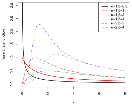
Figure 1. The hazard rate function.

In Section 2, we will discuss some basic characters of $C_L$ as well as the relationship between the product qualification ratio and the lifetime performance index. In Section 3, attention will be paid to the Maximum Likelihood Estimation (MLE) of $C_L$ using Fisher information matrix. In Section 4, we study normal approximation of the MLE and the log-transformed MLE. Then, Section 5 will use the Bayesian method to estimate $C_L$ with the help of Lindley approximation and Monte Carlo Markov Chain method. Section 6 and Section 7 contain simulation studies and an illustrative example. Optimal censoring plan will be discussed in Section 8. In Section 9, some conclusions will be summarized.

2. The Lifetime Performance Index ${\mathit{C}}_{\mathit{L}}$

Let X represent the lifetime of the products. The $C_{L_X}$ (the specific value of $C_L$ when using the random variable X) is defined in Reference [3] as follows:

$$\begin{array}{c}\hfill C_{L_X}=\frac{{\mu }_X-L_X}{{\sigma }_X}\end{array}$$

(4)

where ${\mu }_X$ is the mean of X and ${\sigma }_X$ is the standard deviation of X. $L_X$, the lower specification limit predetermined according to the market demands, specifies the minimum acceptable life of the product. Note that random variable X follows a log-logistic distribution throughout the whole paper. Since the pdf and the cdf of log-logistic distribution are presented earlier as in Equations (1) and (2), we can easily calculate that ${\mu }_X=E(X)=\frac{\alpha b}{sinb}$ and ${\sigma }_X=\sqrt{Var(X)}={\alpha }^2(\frac{2b}{sin2b}-\frac{b^2}{{sin}^{2}b})$, where $\alpha >0$, $\beta >2$ and $b=\frac{\pi }{\beta }$. Then, from Equation (4), the lifetime performance index is

$$\begin{array}{c}\hfill C_{L_X}=\frac{1}{A}(\frac{b}{sinb}-\frac{L_X}{\alpha }),-\infty <C_{L_X}<\sqrt{\frac{b}{tanb-b}}\end{array}$$

(5)

Here, we have $A=\sqrt{\frac{2b}{sin2b}-\frac{b^2}{{sin}^{2}b}}$. It is evident that $C_{L_X}>0$ while $L_X<\frac{\alpha b}{sinb}$. According to Equations (3) and (5), we can conservatively draw the conclusion that it is rational for $C_{L_X}$ to represent the lifetime performance of products since the hazard rate function $r(x,\alpha ,\beta )$ and $C_{L_X}$ have the opposite performance when $\alpha$ increases.

In this paper, a product is assumed to be qualified (subquality) when $X>(<)L_X$. We define the product qualification rate $P_r$, which is also named as the conforming rate, as follows:

$$\begin{array}{c}\hfill P_r=P(X\ge L_X)=\frac{1}{1+{(\frac{b}{sinb}-A{C}_{L_X})}^{\beta }},-\infty <C_{L_X}<\sqrt{\frac{b}{tanb-b}}\end{array}$$

(6)

Visibly, a strictly monotonic increasing relationship exits between $P_r$ and $C_{L_X}$ for given $\beta >2$.

All in all, $C_{L_X}$ has great practical relevance because it can represent the lifetime performance of products and can calculate the theoretical value of conforming rate $P_r$.

3. Maximum Likelihood Estimation for ${\mathit{C}}_{{\mathit{L}}_{\mathit{X}}}$

Based on progressive first-failure-censored samples, the maximum likelihood estimation (MLE) for $\alpha$, $\beta$, and $C_{L_X}$ with log-logistic distribution are analysed in this section. Firstly, let $X_{1:m:n}\le X_{2:m:n}\le \cdots \le X_{m:m:n}$ be the sample generated from the log-logistic distribution following censoring schemes $(R_1,\cdots ,R_m)$. Then, under this progressive first-failure-censored sample, the joint pdf based on the abovementioned censoring scheme is

$$\begin{array}{c}\hfill f_{X_{1:m:n}\le X_{2:m:n}\le \cdots \le X_{m:m:n}}(x_1,x_2,\cdots x_m)=B{k}^m{\displaystyle \prod _{i=1}^m}f(x_{i:m:n})\times {[1-F(x_{i:m:n})]}^{k(R_i+1)-1},\end{array}$$

(7)

where $B=n(n-R_1-1)\cdots (n-R_1-\cdots -R_{m-1}-m+1)$ is a normal constant and $0<x_1<x_2<\cdots <x_m<+\infty$ is obligatory.

Substituting Equations (1) and (2) into Equation (7), we get the likelihood function ($lf$):

$$\begin{array}{c}\hfill L(\alpha ,\beta )=B{k}^m{\beta }^m{\alpha }^{\beta k{\sum }_{i=1}^m(R_i+1)}{\displaystyle \prod _{i=1}^m}{\displaystyle \frac{x_i^{\beta -1}}{{({\alpha }^{\beta }+x_i^{\beta })}^{k(R_i+1)+1}}}\end{array}$$

(8)

Both $\alpha$ and $\beta$ are assumed to be unknown for further discussion. Take the logarithm of Equation (8) and the log-likelihood function $l(\alpha ,\beta ,x)$ becomes the following:

$$\begin{array}{c}\hfill l=logB+mlogk\beta +\beta klog\alpha \times {\displaystyle \sum _{i=1}^m}(R_i+1)+(\beta -1){\displaystyle \sum _{i=1}^m}ln{x}_i-{\displaystyle \sum _{i=1}^m}[k(R_i+1)+1]log({\alpha }^{\beta }+x_i^{\beta })\end{array}$$

$l(\alpha ,\beta ,x)$ differentiates $\alpha$ and $\beta$ respectively, and we can get the following:

$$\begin{array}{c}\hfill \frac{\partial l}{\partial \alpha }=\frac{\beta }{\alpha }{\displaystyle \sum _{i=1}^m}k(R_i+1)-{\displaystyle \sum _{i=1}^m}[k(R_i+1)+1]{\displaystyle \frac{\beta {\alpha }^{\beta -1}}{{\alpha }^{\beta }+x_i^{\beta }}}\end{array}$$

(9)

$$\begin{array}{c}\hfill \frac{\partial l}{\partial \beta }=\frac{m}{\beta }+kln\alpha {\displaystyle \sum _{i=1}^m}(R_i+1)+{\displaystyle \sum _{i=1}^m}ln{x}_i-{\displaystyle \sum _{i=1}^m}[k(R_i+1)+1]\frac{{\alpha }^{\beta }log(\alpha )+x^{\beta }log(x)}{{\alpha }^{\beta }+x^{\beta }}\end{array}$$

(10)

Set the above two Equations (9) and (10) to zero, and the MLEs of $\alpha$ and $\beta$ can be obtained through calculation. From Equation (9), we can observe the following:

$$\begin{array}{c}\hfill \alpha ={\left(\frac{W}{m}\right)}^{\frac{1}{\beta }}\end{array}$$

(11)

where $W={\sum }_{i=1}^{m}k(R_i+1)x_i^{\beta }$.

Then, substitute the value of $\alpha$ from Equation (11) into Equation (10):

$$\begin{array}{c}\hfill \frac{m}{\beta }+{\displaystyle \sum _{i=1}^m}{\displaystyle \frac{W}{W+m{x}_i^{\beta }}}(ln{x}_i-\frac{1}{\beta }ln\frac{W}{m})-{\displaystyle \sum _{i=1}^m}k(R_i+1){\displaystyle \frac{m{x}_i^{\beta }}{W+md{x}_i^{\beta }}}(ln{x}_i-\frac{1}{\beta }ln\frac{W}{m})=0\end{array}$$

(12)

Choosing a suitable iterative procedure, the solution to Equation (12) can be evaluated numerically when values of $(k,n,m,R,x)$ are given. Let the MLE of $\beta$ be $\widehat{\beta }$, and the MLE of b can be obtained as $\widehat{b}={\displaystyle \frac{\pi }{\widehat{\beta }}}$. Then, it is available to get $\widehat{\alpha }$, the MLE of $\alpha$, by substituting $\widehat{\beta }$ into Equation (11). Due to the invariance property, the MLE of $C_{L_X}$ is obtained as follows:

$$\begin{array}{c}\hfill \widehat{C_{L_X}}=\frac{1}{\widehat{A}}(\frac{\widehat{b}}{sin\widehat{b}}-\frac{L_X}{\widehat{\alpha }})\end{array}$$

(13)

4. Confidence Intervals

4.1. Asymptotic Confidence Intervals for MLE

Let $\theta =(\alpha ,\beta )$, and the Fisher information matrix of $\theta$ is as follows:

$$\begin{array}{c}\hfill \mathrm{I}(\theta )=E\left[\begin{array}{cc}-{\displaystyle \frac{{\partial }^{2}l}{\partial {\alpha }^2}}& -{\displaystyle \frac{{\partial }^{2}l}{\partial \alpha \partial \beta }}\\ -{\displaystyle \frac{{\partial }^{2}l}{\partial \beta \partial \alpha }}& -{\displaystyle \frac{{\partial }^{2}l}{\partial {\beta }^2}}\end{array}\right].\end{array}$$

(14)

The specific expressions of sencond derivatives of l are presented in Appendix A.

It is infeasible to derive the expectation of above expressions; henceforward, the observed Fisher information matrix is utilized for calculation. Set $\widehat{\theta }=(\widehat{\alpha },\widehat{\beta })$ to be the MLE of $\theta =(\alpha ,\beta )$. When $\theta =\widehat{\theta }=(\widehat{\alpha },\widehat{\beta })$, the inverse of Equation (14) is the observed variance–covariance matrix of MLEs:

$$\begin{array}{c}\hfill {\mathrm{I}}^{-1}(\widehat{\theta })={\left(\begin{array}{cc}\widehat{Var}(\widehat{\alpha })& \widehat{Cov}(\widehat{\alpha },\widehat{\beta })\\ \widehat{Cov}(\widehat{\beta },\widehat{\alpha })& \widehat{Var}(\widehat{\beta })\end{array}\right)}_{\theta =\widehat{\theta }}\end{array}$$

(15)

With mean as $(\alpha ,\beta )$ and covariance matrix as $I^{-1}(\alpha ,\beta )$, the asymptotic distribution of MLEs $\widehat{\theta }$ is approximately bivariately normal; $100(1-\zeta )\%$ two-tailed asymptotic confidence intervals of $\alpha$ and $\beta$ are respectively the following:

$$\begin{array}{c}\hfill \widehat{\alpha }\pm {\mathrm{Z}}_{\zeta /2}\sqrt{\widehat{Var}(\widehat{\alpha })}and\widehat{\beta }\pm {\mathrm{Z}}_{\zeta /2}\sqrt{\widehat{Var}(\widehat{\beta })}\end{array}$$

(16)

The $\zeta /2$ percentile of the standard normal distribution is $Z_{\zeta /2}$. Then, applying Monte Carlo simulation, the coverage probabilities (CPs) of $\alpha$ and $\beta$ are respectively

$$C{P}_{\alpha }=P\left[|{\displaystyle \frac{(\widehat{\alpha }-\alpha )}{\sqrt{\widehat{Var}(\widehat{\alpha })}}}|\le {\mathrm{Z}}_{\zeta /2}\right]andC{P}_{\beta }=P\left[|{\displaystyle \frac{(\widehat{\beta }-\beta )}{\sqrt{\widehat{Var}(\widehat{\beta })}}}|\le {\mathrm{Z}}_{\zeta /2}\right]$$

.

In addition, we assume that $R^{\mathrm{T}}=({\displaystyle \frac{\partial C_{L_X}}{\partial \alpha }},{\displaystyle \frac{\partial C_{L_X}}{\partial \beta }})$ and we have the following:

$$\begin{array}{c}\hfill {\displaystyle \frac{\partial C_{L_X}}{\partial \alpha }}=\frac{L_X}{{\alpha }^2\sqrt{\frac{2\pi csc\left(\frac{2\pi }{\beta }\right)}{\beta }-\frac{{\pi }^2{csc}^2\left(\frac{\pi }{\beta }\right)}{{\beta }^2}}},\end{array}$$

$$\begin{array}{ccc}\hfill \frac{\partial C_{L_X}}{\partial \beta }& =& \mathbb{M}-C_{L_X}\mathbb{N}\hfill \end{array}$$

where

$$\begin{array}{cc}\hfill \mathbb{M}=& {\displaystyle \frac{\frac{{\pi }^{2}cot\left(\frac{\pi }{\beta }\right)csc\left(\frac{\pi }{\beta }\right)}{{\beta }^3}-\frac{\pi csc\left(\frac{\pi }{\beta }\right)}{{\beta }^2}}{\sqrt{\frac{2\pi csc\left(\frac{2\pi }{\beta }\right)}{\beta }-\frac{{\pi }^2{csc}^2\left(\frac{\pi }{\beta }\right)}{{\beta }^2}}}}\hfill \\ \hfill \mathbb{N}=& {\displaystyle \frac{\left(-\frac{2{\pi }^{3}cot\left(\frac{\pi }{\beta }\right){csc}^2\left(\frac{\pi }{\beta }\right)}{{\beta }^4}+\frac{2{\pi }^2{csc}^2\left(\frac{\pi }{\beta }\right)}{{\beta }^3}+\frac{4{\pi }^{2}cot\left(\frac{2\pi }{\beta }\right)csc\left(\frac{2\pi }{\beta }\right)}{{\beta }^3}-\frac{2\pi csc\left(\frac{2\pi }{\beta }\right)}{{\beta }^2}\right)}{2\left(\frac{2\pi csc\left(\frac{2\pi }{\beta }\right)}{\beta }-\frac{{\pi }^2{csc}^2\left(\frac{\pi }{\beta }\right)}{{\beta }^2}\right)}}\hfill \end{array}$$

Then, we define the asymptotic estimator of $\widehat{Var}(\widehat{C_{L_X}})$ as follows:

$$\begin{array}{c}\hfill \widehat{Var}(\widehat{C_{L_X}})\simeq {\left[R^{\mathrm{T}}{I}^{-1}R\right]}_{(\alpha ,\beta )=(\widehat{\alpha },\widehat{\beta })}\end{array}$$

Using the delta method, we know that

$$\begin{array}{c}\hfill {\displaystyle \frac{\widehat{C_{L_X}}-C_{L_X}}{\sqrt{\widehat{Var}(\widehat{C_{L_X}})}}}\sim N(0,1)\end{array}$$

Thus, the $100(1-\zeta )\%$ asymptotic confidence interval of $C_{L_X}$ can be derived as

$$\begin{array}{c}\hfill \widehat{C_{L_X}}\pm {\mathrm{Z}}_{\zeta /2}\sqrt{\widehat{Var}(\widehat{C_{L_X}})}\end{array}$$

(17)

4.2. Asymptotic Confidence Intervals for the Log-Transformed MLE

According to References [8,24], the asymptotic confidence intervals has better CP using log-transformed MLE. The $100(1-\zeta )\%$ asymptotic confidence intervals of $\alpha$ and $\beta$ for the log-transformed MLE are

$$\begin{array}{ccc}\hfill log\widehat{\alpha }\pm {\mathrm{Z}}_{\zeta /2}\sqrt{\widehat{Var}(\widehat{log\widehat{\alpha }})}& and& log\widehat{\beta }\pm {\mathrm{Z}}_{\zeta /2}\sqrt{\widehat{Var}(\widehat{log\widehat{\beta }})}\hfill \end{array}$$

The $100(1-\zeta )\%$ approximate confidence intervals of $\alpha$ and $\beta$ for log-transformed MLE are

$$\begin{array}{ccc}\hfill \widehat{\alpha }exp[\pm \frac{{\mathrm{Z}}_{\zeta /2}\sqrt{\widehat{Var}(\widehat{\alpha })}}{\widehat{\alpha }}]& and& \widehat{\beta }exp[\pm \frac{{\mathrm{Z}}_{\zeta /2}\sqrt{\widehat{Var}(\widehat{\beta })}}{\widehat{\beta }}]\hfill \end{array}$$

(18)

Similarly, the $100(1-\zeta )\%$ normal approximation confidence interval of $C_{L_X}$ is

$$\begin{array}{c}\hfill \widehat{C_{L_X}}exp[\pm \frac{{\mathrm{Z}}_{\zeta /2}\sqrt{\widehat{Var}(\widehat{C_{L_X}})}}{\widehat{C_{L_X}}}].\end{array}$$

(19)

5. Bayesian Estimation

5.1. Prior Distribution and Posterior Analysis

A more precise and efficient method is considered to obtain approximate estimators of $\alpha$ and $\beta$ here. First of all, prior distributions used in calculation are Gamma distributions:

$$\begin{array}{c}{g}_1(\alpha )\sim {\alpha }^{a_1-1}{e}^{-b_1\alpha },\alpha >0,a_1>0,b_1>0\\ g_2(\beta )\sim {\beta }^{a_2-1}{e}^{-b_2\beta },\beta >2,a_2>0,b_2>0\end{array}$$

The joint prior distribution is

$$\begin{array}{c}\hfill \pi (\alpha ,\beta )\sim {\alpha }^{a_1-1}{\beta }^{a_2-1}{e}^{-(b_1\alpha +b_2\beta )}\end{array}$$

(20)

The joint posterior distribution is

$$\begin{array}{cc}\hfill \pi (\alpha ,\beta |x)& =\frac{\pi (\alpha ,\beta )L(x|\alpha ,\beta )}{{\int }_0^{\infty }{\int }_2^{\infty }\pi (\alpha ,\beta )L(x|\alpha ,\beta )d\alpha d\beta }\hfill \\ \hfill & =\frac{1}{K}{\alpha }^{{\gamma }_1-1}{\beta }^{{\gamma }_2-1}{e}^{-(b_1\alpha +b_2\beta )}{\displaystyle \prod _{i=1}^m}\frac{x_i^{\beta -1}}{{({\alpha }^{\beta }+x_i^{\beta })}^{k(R_i+1)+1}}\hfill \end{array}$$

(21)

where

$$\begin{array}{cc}\hfill & K={\int }_0^{\infty }{\int }_2^{\infty }{\alpha }^{{\gamma }_1-1}{\beta }^{{\gamma }_2-1}{e}^{-(b_1\alpha +b_2\beta )}{\displaystyle \prod _{i=1}^m}\frac{x_i^{\beta -1}}{{({\alpha }^{\beta }+x_i^{\beta })}^{k(R_i+1)+1}}d\alpha d\beta .\hfill \\ \hfill & {\gamma }_1=\beta {\displaystyle \sum _{i=1}^m}k(R_i+1)+a_1,{\gamma }_2=m+a_2\hfill \end{array}$$

5.2. Asymmetric and Symmetric Loss Functions

In the Bayesian estimation, the loss function is of great importance. The Bayesian estimation for parameters $\alpha$ and $\beta$ and lifetime performance index $C_{L_X}$ from a log-logistic distribution under both asymmetric as well as symmetric loss functions are carried out. The loss functions we chose are widely studied: the squared error loss function (SELF), the linex loss function (LF), the general entropy loss function (GELF). Their definitions are as follows:

$$\begin{array}{cc}\hfill L_{SELF}(\eta ,\widehat{\eta })& ={(\widehat{\eta }-\eta )}^2\hfill \\ \hfill L_{LF}(\eta ,\widehat{\eta })& =e^{\psi (\widehat{\eta }-\eta )}-\psi (\widehat{\eta }-\eta )-1\hfill \\ \hfill L_{GELF}(\eta ,\widehat{\eta })& ={(\frac{\widehat{\eta }}{\eta })}^{\phi }-\phi log\frac{\widehat{\eta }}{\eta }-1\hfill \end{array}$$

Note that $\widehat{\eta }$ represents an estimate of $\eta$, $\psi \ne 0$, and $\phi \ne 0$. In LF and GELF, the positive and negative natures of $\psi$ and $\phi$ show the direction of the asymmetry and the value size shows the degree of asymmetry.

The Bayesian estimation of $\eta$ under SELF, LF, and GELF are respectively as follows:

$$\begin{array}{c}\hfill {\widehat{\eta }}_{SELF}=E_{\eta }\left[\eta \right|\mathrm{X}]\end{array}$$

$$\begin{array}{c}\hfill {\widehat{\eta }}_{LF}=-\frac{1}{\psi }log(E_{\eta }\left[e^{-\psi \eta }\right|\mathrm{X}])\end{array}$$

$$\begin{array}{c}\hfill {\widehat{\eta }}_{GELF}={\left[E_{\eta }\left[{\eta }^{-\phi }\right|\mathrm{X}]\right]}^{-\frac{1}{\phi }}\end{array}$$

The Bayesian estimation under SELF, LF, and GELF of any given function of $\alpha$ and $\beta$, let us say $\varphi (\alpha ,\beta )$, are

$$\begin{array}{c}\hfill \widehat{\varphi }{(\alpha ,\beta )}_{SELF}={\displaystyle \frac{{\int }_0^{\infty }{\int }_2^{\infty }\varphi (\alpha ,\beta )\Im d\alpha d\beta }{{\int }_0^{\infty }{\int }_2^{\infty }\Im d\alpha d\beta }}\end{array}$$

$$\begin{array}{c}\hfill \widehat{\varphi }{(\alpha ,\beta )}_{LF}=-\frac{1}{\psi }log\left({\displaystyle \frac{{\int }_0^{\infty }{\int }_2^{\infty }{e}^{-\psi \varphi (\alpha ,\beta )}\Im d\alpha d\beta }{{\int }_0^{\infty }{\int }_2^{\infty }\Im d\alpha d\beta }}\right)\end{array}$$

$$\begin{array}{c}\hfill \widehat{\varphi }{(\alpha ,\beta )}_{GELF}={\left({\displaystyle \frac{{\int }_0^{\infty }{\int }_2^{\infty }\varphi {(\alpha ,\beta )}^{-\phi }\Im d\alpha d\beta }{{\int }_0^{\infty }{\int }_2^{\infty }\Im d\alpha d\beta }}\right)}^{-\frac{1}{\phi }}\end{array}$$

where $\Im =\pi (\alpha ,\beta )\times L(x|\alpha ,\beta )$.

Clearly, it is infeasible to get the accurate closed form of the Bayesian estimation. Hence, Lindley method is used in the next section to derive the Bayes estimator.

5.3. Lindley Approximation Method

Lindley approximation method is introduced by Reference [25] to approximate two integral ratios. According to this method, the Bayes estimate of any function of $({\wp }_1,{\wp }_2)$, $\varphi ({\wp }_1,{\wp }_2)$, is

$$\widehat{\varphi }=\varphi (\widehat{{\wp }_1},\widehat{{\wp }_2})+0.5(E+l_{30}{F}_{12}+l_{03}{F}_{21}+l_{21}{G}_{12}+l_{12}{G}_{21})+{\rho }_1{E}_{12}+{\rho }_2{E}_{21}$$

(22)

where

$$\begin{array}{cc}\hfill & E={\displaystyle \sum _{i=1}^2}{\displaystyle \sum _{j=1}^2}{\varphi }_{ij}{\tau }_{ij},E_{ij}={\varphi }_i{\tau }_{ii}+{\varphi }_j{\tau }_{ji},l_{ij}=\frac{{\partial }^{i+j}l({\wp }_1,{\wp }_2)}{\partial {\wp }_1^i\partial {\wp }_2^j}\hfill \\ \hfill & F_{ij}=({\varphi }_i{\tau }_{ii}+{\varphi }_j{\tau }_{ji}){\sigma }_{ii}{G}_{ij}=3{\varphi }_{ij}{\tau }_{ii}{\tau }_{jj}+{\varphi }_j({\tau }_{ii}{\tau }_{jj}+2{\tau }_{ij}^2),\hfill \\ \hfill & {\rho }_i=\frac{\partial \rho }{\partial {\wp }_i},\rho =log\pi ({\wp }_1,{\wp }_2)\hfill \\ \hfill & {\varphi }_i=\frac{\partial \varphi }{\partial {\wp }_i},{\varphi }_{ij}=\frac{{\partial }^2\varphi }{\partial {\wp }_i\partial {\wp }_j}i,j=1,2\hfill \\ \hfill & {\rho }_1=\frac{\partial \rho }{\partial \alpha }=\frac{a_1-1}{\alpha }-b_1,{\rho }_2=\frac{\partial \rho }{\partial \beta }=\frac{a_2-1}{\beta }-b_2\hfill \end{array}$$

The specific expressions of $l_{ij}$ (also known as third derivatives of l) are presented in Appendix B. ${\tau }_{ij}$ represents the $(i,j)$th element from the observed variance–covariance matrix in Equation (15) calculated in Section 4.1. We calculate $\widehat{\varphi }$ for the estimation of (${\wp }_1$, ${\wp }_2$) = ($\alpha$, $\beta$).

5.3.1. The Squared Error Loss Function (SELF)

Taking $\varphi (\alpha ,\beta )=\alpha$, $\beta$ and $C_{L_X}$, first of all, the Bayes estimator of $\alpha$ and $\beta$ under SELF can be obtained respectively as

$$\begin{array}{cc}\hfill {\widehat{\alpha }}_{LB}& =\widehat{\alpha }+{\rho }_1{\tau }_{11}+{\rho }_2{\tau }_{12}+0.5\left[{\tau }_{11}(l_{30}{\tau }_{11}+2l_{21}{\tau }_{12}+l_{12}{\tau }_{22})+{\tau }_{21}(l_{21}{\tau }_{11}+2l_{12}{\tau }_{21}+l_{03}{\tau }_{22})\right]\hfill \\ \hfill {\widehat{\beta }}_{LB}& =\widehat{\beta }+{\rho }_1{\tau }_{21}+{\rho }_2{\tau }_{22}+0.5\left[{\tau }_{12}(l_{30}{\tau }_{11}+2l_{21}{\tau }_{12}+l_{12}{\tau }_{22})+{\tau }_{22}(l_{21}{\tau }_{11}+2l_{12}{\tau }_{21}+l_{03}{\tau }_{22})\right]\hfill \end{array}$$

Similarly, we take $\varphi (\alpha ,\beta )=C_{L_X}$, and the Bayes estimator of $C_{L_X}$ can be obtained as follows:

$$\begin{array}{cc}\hfill {\widehat{C}}_{L_{X_{SELF}}}=& {\widehat{C}}_{L_X}+0.5\left[({\widehat{\varphi }}_{11}+2{\widehat{\varphi }}_1{\widehat{\rho }}_1){\widehat{\tau }}_{11}+({\widehat{\varphi }}_{12}+2{\widehat{\varphi }}_1{\widehat{\rho }}_2){\widehat{\tau }}_{12}+({\widehat{\varphi }}_{21}+2{\widehat{\varphi }}_2{\widehat{\rho }}_1){\widehat{\tau }}_{21}\right.\hfill \\ \hfill +& ({\widehat{\varphi }}_{22}+2{\widehat{\varphi }}_2{\widehat{\rho }}_2){\widehat{\tau }}_{22}+({\widehat{\varphi }}_1{\widehat{\tau }}_{11}+{\widehat{\varphi }}_2{\widehat{\tau }}_{12})({\widehat{l}}_{30}{\widehat{\tau }}_{11}+2{\widehat{l}}_{21}{\widehat{\tau }}_{12}+{\widehat{l}}_{12}{\widehat{\tau }}_{22})\hfill \\ \hfill +& \left.({\widehat{\varphi }}_1{\widehat{\tau }}_{21}+{\widehat{\varphi }}_2{\widehat{\tau }}_{22})({\widehat{l}}_{21}{\widehat{\tau }}_{11}+2{\widehat{l}}_{12}{\widehat{\tau }}_{21}+{\widehat{l}}_{03}{\widehat{\tau }}_{22})\right]\hfill \end{array}$$

The specific expressions of ${\varphi }_i$ and ${\varphi }_{ij}$ under SELF are presented in Appendix C.1.

5.3.2. The Linex Loss Function (LF)

For $\alpha$, taking $\varphi (\alpha ,\beta )=e^{-\psi \alpha }$, we obtain that

$$\begin{array}{c}\hfill {\varphi }_1=-\psi e^{-\psi \alpha },{\varphi }_{11}={\psi }^2{e}^{-\psi \alpha },{\varphi }_2={\varphi }_{12}={\varphi }_{21}={\varphi }_{22}=0.\end{array}$$

(23)

Substituting Equation (23) into Equation (22), the Bayes estimator of $\alpha$ under LF is

$$\begin{array}{cc}\hfill {\widehat{\alpha }}_{LF}=-& \frac{1}{\psi }log\left[e^{-\psi \widehat{\alpha }}+0.5({\psi }^2{e}^{-\psi \alpha }{\tau }_{11}-\psi e^{-\psi \alpha }(2{\rho }_1{\tau }_{11}+2{\rho }_2{\tau }_{12}\right.\hfill \\ \hfill +& \left.{\tau }_{11}(l_{30}{\tau }_{11}+2l_{21}{\tau }_{12}+l_{12}{\tau }_{22})+{\tau }_{21}(l_{21}{\tau }_{11}+2l_{12}{\tau }_{21}+l_{03}{\tau }_{22})))\right]\hfill \end{array}$$

Similarly, taking $\varphi (\alpha ,\beta )=e^{-\psi \beta }$, we can obtain that

$$\begin{array}{c}\hfill {\varphi }_2=-\psi e^{-\psi \beta },{\varphi }_{22}={\psi }^2{e}^{-\psi \beta },{\varphi }_1={\varphi }_{11}={\varphi }_{21}={\varphi }_{12}=0.\end{array}$$

The Bayes estimator of $\beta$ according to Equation (22) under LF is

$$\begin{array}{cc}\hfill {\widehat{\beta }}_{LF}=-& \frac{1}{\psi }log\left[e^{-\psi \widehat{\beta }}+0.5({\psi }^2{e}^{-\psi \beta }{\tau }_{22}-\psi e^{-\psi \beta }(2{\rho }_1{\tau }_{21}+2{\rho }_2{\tau }_{22}\right.\hfill \\ \hfill +& \left.{\tau }_{12}(l_{30}{\tau }_{11}+2l_{21}{\tau }_{12}+l_{12}{\tau }_{22})+{\tau }_{22}(l_{21}{\tau }_{11}+2l_{12}{\tau }_{21}+l_{03}{\tau }_{22})))\right]\hfill \end{array}$$

Then, we compute the Bayesian estimation of $C_{L_X}$ under LF when $\varphi (\alpha ,\beta )=e^{-\psi C_{L_X}}$ is

$$\begin{array}{cc}{\widehat{C}}_{L_{X_{LF}}}=\hfill & -\frac{1}{\psi }log\left[e^{-\psi {\widehat{C}}_{L_X}}+0.5(({\varphi }_{11}+2{\varphi }_1{\rho }_1){\tau }_{11}+({\varphi }_{12}+2{\varphi }_1{\rho }_2){\tau }_{12}+({\varphi }_{21}+2{\varphi }_2{\rho }_1){\tau }_{21}\right.\hfill \\ & +({\varphi }_{22}+2{\varphi }_2{\rho }_2){\tau }_{22}+({\varphi }_1{\tau }_{11}+{\varphi }_2{\tau }_{12})(l_{30}{\tau }_{11}+2l_{21}{\tau }_{12}+l_{12}{\tau }_{22})\hfill \\ & +\left.({\varphi }_1{\tau }_{21}+{\varphi }_2{\tau }_{22})(l_{21}{\tau }_{11}+2l_{12}{\tau }_{21}+l_{03}{\tau }_{22}))\right]\hfill \end{array}$$

The specific expressions of ${\varphi }_i$ and ${\varphi }_{ij}$ under LF are presented in Appendix C.2.

5.3.3. The General Entropy Loss Function (GELF)

Taking $\varphi (\alpha ,\beta )$= ${\alpha }^{-\phi }$, we calculate that

$$\begin{array}{c}\hfill {\varphi }_1=-\phi {\alpha }^{-\phi -1},{\varphi }_{11}=\phi (\phi +1){\alpha }^{-\phi -2},{\varphi }_{12}={\varphi }_{21}={\varphi }_2={\varphi }_{22}=0\end{array}$$

Then, we can get the Bayesian estimation of $\alpha$ under GELF as

$$\begin{array}{cc}\hfill {\widehat{\alpha }}_{GELF}& =\left[{\widehat{\alpha }}^{-\phi }+0.5(\phi (\phi +1){\alpha }^{-\phi -2}{\tau }_{11}-\phi {\alpha }^{-\phi -1}(2{\rho }_1{\tau }_{11}+2{\rho }_2{\tau }_{12}\right.\hfill \\ \hfill +& {\left.{\tau }_{11}(l_{30}{\tau }_{11}+2l_{21}{\tau }_{12}+l_{12}{\tau }_{22})+{\tau }_{21}(l_{21}{\tau }_{11}+2l_{12}{\tau }_{21}+l_{03}{\tau }_{22})))\right]}^{-\frac{1}{\phi }}\hfill \end{array}$$

Taking $\varphi (\alpha ,\beta )={\beta }^{-\phi }$, we have

$$\begin{array}{c}\hfill {\varphi }_2=-\phi {\beta }^{-\phi -1},{\varphi }_{22}=\phi (\phi +1){\beta }^{-\phi -2},{\varphi }_{12}={\varphi }_{21}={\varphi }_1={\varphi }_{11}=0\end{array}$$

Then, we can get the Bayesian estimation of $\beta$ under GELF as

$$\begin{array}{cc}\hfill {\widehat{\beta }}_{GELF}=& \left[{\widehat{\beta }}^{-\phi }+0.5(\phi (\phi +1){\beta }^{-\phi -2}{\tau }_{22}-\phi {\beta }^{-\phi -1}(2{\rho }_1{\tau }_{21}+2{\rho }_2{\tau }_{22}\right.\hfill \\ \hfill +& {\left.{\tau }_{12}(l_{30}{\tau }_{11}+2l_{21}{\tau }_{12}+l_{12}{\tau }_{22})+{\tau }_{22}(l_{21}{\tau }_{11}+2l_{12}{\tau }_{21}+l_{03}{\tau }_{22})))\right]}^{-\frac{1}{\phi }}\hfill \end{array}$$

Similarly, taking $\varphi (\alpha ,\beta )=C_{L_X}^{-\phi }$, the Bayes estimate of $C_{L_X}$ under GELF is

$$\begin{array}{cc}\hfill \widehat{C_{L_{X_{GELF}}}}=& \left[{\widehat{C}}_{L_X}^{-\phi }+0.5(({\varphi }_{11}+2{\varphi }_1{\rho }_1){\tau }_{11}+({\varphi }_{12}+2{\varphi }_1{\rho }_2){\tau }_{12}+({\varphi }_{21}+2{\varphi }_2{\rho }_1){\tau }_{21}\right.\hfill \\ & +({\varphi }_{22}+2{\varphi }_2{\rho }_2){\tau }_{22}+({\varphi }_1{\tau }_{11}+{\varphi }_2{\tau }_{12})(l_{30}{\tau }_{11}+2l_{21}{\tau }_{12}+l_{12}{\tau }_{22})\hfill \\ & +{\left.({\varphi }_1{\tau }_{21}+{\varphi }_2{\tau }_{22})(l_{21}{\tau }_{11}+2l_{12}{\tau }_{21}+l_{03}{\tau }_{22}))\right]}^{-\frac{1}{\phi }}\hfill \end{array}$$

The specific expressions of ${\varphi }_i$ and ${\varphi }_{ij}$ under GELF are presented in Appendix C.3.

The Bayes estimator of parameters $\alpha$ and $\beta$ and the lifetime performance index $C_{L_X}$ can be obtained using the Lindley method. Unfortunately, the Higher Posterior Density (HPD) credible intervals could not be studied since the Lindley approximation method only makes the point estimation. That is what we are going to focus on in the next section.

5.4. Monte Carlo Markov Chain Method

When estimating intricate Bayesian models, Monte Carlo Markov Chain (MCMC) is an effective method and have been used for research by many scholars; see Reference [16,26]. Metropolis–Hastings algorithm is the most commonly used Monte Carlo Markov Chain method in statistics, digital communication, signal processing, and other fields. In this paper, a mixed strategy combining the Metropolis–Hastings algorithm within the type of random walk chain is utilized for generating progressive first-failure-censored samples from each posterior distribution arising from log-logistic distribution. We apply the R function rwmetrop in the LearnBayes package. Reference [27] gave a detailed description.

From Equation (21), we acquire the joint posterior distributions of $\alpha$ and $\beta$:

$$\begin{array}{cc}\hfill \pi (\alpha ,\beta |x)& \sim {\alpha }^{{\gamma }_1-1}{e}^{-b_1\alpha }{\beta }^{{\gamma }_2-1}{e}^{-b_2\beta }{\displaystyle \prod _{i=1}^m}\frac{x_i^{\beta -1}}{{({\alpha }^{\beta }+x_i^{\beta })}^{k(R_i+1)+1}}\hfill \\ \hfill & \sim \frac{b_1^{{\gamma }_1}}{\Gamma ({\gamma }_1)}{\alpha }^{{\gamma }_1-1}{e}^{-b_1\alpha }\times \frac{b_2^{{\gamma }_2}}{\Gamma ({\gamma }_2)}{\beta }^{{\gamma }_2-1}{e}^{-b_2\beta }{\displaystyle \prod _{i=1}^m}\frac{x_i^{\beta -1}}{{({\alpha }^{\beta }+x_i^{\beta })}^{k(R_i+1)+1}}\hfill \\ \hfill \pi (\alpha ,\beta |x)& \sim {\pi }_1(\alpha |\beta ,x)\times {\pi }_2(\beta |\alpha ,x).\hfill \end{array}$$

Here, we have

$$\begin{array}{ccc}\hfill {\pi }_1(\alpha |\beta ,x)& =& Gamma({\gamma }_1,b_1)=\frac{b_1^{{\gamma }_1}}{\Gamma ({\gamma }_1)}{\alpha }^{{\gamma }_1-1}{e}^{-b_1\alpha }\hfill \\ \hfill {\pi }_2(\beta |\alpha ,x)& =& \frac{b_2^{{\gamma }_2}}{\Gamma ({\gamma }_2)}{\beta }^{{\gamma }_2-1}{e}^{-\beta (b_2-{\sum }_{i=1}^{m}ln{x}_i)}{\displaystyle \prod _{i=1}^m}{\displaystyle \frac{1}{x_i{({\alpha }^{\beta }+x_i^{\beta })}^{k(R_i+1)+1}}}\hfill \end{array}$$

Since ${\pi }_1(\alpha |\beta ,x)$ is a standard gamma density function, samples of $\alpha$ can be easily generated. Unfortunately, ${\pi }_2(\beta |\alpha ,x)$ cannot be simplified to the widely studied distributions. Consequently, the required random samples are generated from the conditional posterior density by applying the Metropolis–Hastings method and the process is as follows:

Step  1:

Initialize the values of $({\alpha }_1,{\beta }_1)$.

Step 2:

Set the initial value of t to 1.

Step 3:

Generate ${\alpha }_t$ from $Gamma({\gamma }_1,b_1)$.

Step 4:

Generate ${\beta }_t$ from ${\pi }_2({\beta }_{t-1}|{\alpha }_t,x)$, using the following algorithm:

Step 4-1:

Generate $\dot{\beta }$ from $Normal({\beta }_{t-1},Variance(\beta ))$.

Step 4-2:

Generate $\omega$ from $Uniform(0,1)distribution$.

Step 4-3:

Set ${\beta }_t=\left\{\begin{array}{cc}\dot{\beta }\hfill & if\omega <{\nu }_{\beta }\hfill \\ {\beta }_{t-1}\hfill & if\omega >{\nu }_{\beta }\hfill \end{array}\right.$ and ${\nu }_{\beta }=min(1,{\displaystyle \frac{{\pi }_2(\dot{\beta }|{\alpha }_t,x)}{{\pi }_2{\beta }_{t-1}|{\alpha }_t,x}})$.

Step 5:

t = $t+1$.

Step 6:

Repeat steps 3–5 for M times.

Under SELF, the approximate Bayes estimator of parameters $\alpha$ and $\beta$, and the lifetime performance index $C_{L_X}=\Re ({\alpha }_i,{\beta }_i)$ can be obtained as

$${\widehat{\alpha }}_{MCMC-SE}=\frac{1}{M}{\displaystyle \sum _{i=1}^M}{\alpha }_i{\widehat{\beta }}_{MCMC-SE}=\frac{1}{M}{\displaystyle \sum _{i=1}^M}{\beta }_i{\widehat{C_{L_X}}}_{MCMC-SE}=\frac{1}{M}{\displaystyle \sum _{i=1}^M}\Re ({\alpha }_i,{\beta }_i)$$

HPD credible intervals of parameters $\alpha$ and $\beta$ and the lifetime performance index $C_{L_X}$ can be obtained applying MCMC techniques as follows:

(1) Arrange ${\alpha }_i$ and ${\beta }_i$ as ${\alpha }_1,{\alpha }_2,\cdots ,{\alpha }_M$ and ${\beta }_1,{\beta }_2,\cdots ,{\beta }_M$.

(2) The $(100-\zeta )\%$ symmetric credible intervals of $\alpha$ and $\beta$ are $\left({\alpha }_{M(\zeta /2)},{\alpha }_{M(1-\zeta /2)}\right)$ and $\left({\beta }_{M(\zeta /2)},{\beta }_{M(1-\zeta /2)}\right)$, respectively.

(3) Similarly, the $(100-\zeta )\%$ symmetric credible interval of $C_{L_X}$ is $\left(C_{L_{X_{M(\zeta /2)}}},C_{L_{X_{M(1-\zeta /2)}}}\right)$.

6. Simulation Results

The Monte Carlo simulation study is used for analyzing and comparing the performance of various estimators proposed in the preceding sections. Values of various scale parameters $\alpha$ and $\beta$ and different sample sizes n, group sizes k, effective sample sizes m, and censored schemes $(R_1,R_2,\cdots ,R_m)$ from log-logistic distribution are used in simulation study. Reference [28] proposed referential algorithm for generating the progressive first-failure-censored samples. Briefly summarized, generating the progressive first-failure censored sample with cdf $F(x)$ can be regarded as generating the progressive type-II censored sample with cdf $1-{(1-F(x))}^k$ on calculating. Furthermore, different censoring schemes $(R_1,R_2,\cdots ,R_m)$ presented in the Table 1, Table 2, Table 3, Table 4, Table 5, Table 6, Table 7 and Table 8 are abbreviations. For example, (0*3) denotes (0,0,0) and ((0,1)*2) denotes (0,1,0,1). Note that we use R for simulation study.

Table 1. Maximum Likelihood Estimations (MLEs) of $\alpha$, $\beta$, and $C_L$ when $L=1$, $N=1000$, $\alpha =1.25$, $\beta =1.1\pi$, and $C_L=0.4761017$.

k	n	m	Censoring Scheme	${\widehat{\mathit{\alpha }}}_{\mathbf{ML}}$		${\widehat{\mathit{\beta }}}_{\mathbf{ML}}$		${\widehat{{\mathit{C}}_{\mathit{L}}}}_{\mathbf{ML}}$
				EV ${}^1$	MSE ${}^2$	EV	MSE	EV	MSE
	50	30	(10,0*28,10)	1.2440	0.0091	3.6203	0.3579	0.4656	0.0079
			(1*20,0*10)	1.2414	0.0098	3.6027	0.3014	0.4620	0.0076
			(1*10,0*10,1*10)	1.2369	0.0087	3.6118	0.3305	0.4593	0.0072
		40	(10,0*39)	1.2476	0.0068	3.5585	0.2127	0.4730	0.0062
			(1*10,0*30)	1.2480	0.0073	3.5454	0.2145	0.4707	0.0064
			(0*39,10)	1.2440	0.0065	3.6012	0.2883	0.4704	0.0057
	70	35	(35,0*34)	1.2448	0.0081	3.5508	0.2503	0.4659	0.0072
2			(1*35)	1.2453	0.0083	3.5879	0.2641	0.4654	0.0059
			(0*34,35)	1.2448	0.0089	3.6055	0.3615	0.4606	0.0057
		50	((0,1)*20,1*10)	1.2477	0.0056	3.5354	0.1625	0.4716	0.0045
			(1*20,0*30)	1.2472	0.0062	3.5310	0.1531	0.4705	0.0048
			(0*30,1*20)	1.2443	0.0057	3.5573	0.1998	0.4684	0.0042
	100	50	(25,0*48,25)	1.2472	0.0058	3.5471	0.2007	0.4685	0.0036
			(1*50)	1.2452	0.0053	3.5579	0.1829	0.4690	0.0034
			(0*49,50)	1.2395	0.0065	3.5943	0.2395	0.4636	0.0036
	50	30	(10,0*28,10)	1.2360	0.0098	3.6429	0.3770	0.4558	0.0066
			(1*20,0*10)	1.2442	0.0095	3.5869	0.2668	0.4632	0.0063
			(1*10,0*10,1*10)	1.2398	0.0104	3.6182	0.3441	0.4565	0.0066
		40	(10,0*39)	1.2423	0.0070	3.5580	0.2206	0.4648	0.0054
			(1*10,0*30)	1.2458	0.0069	3.5482	0.1808	0.4679	0.0048
			(0*39,10)	1.2423	0.0073	3.5772	0.2633	0.4630	0.0047
	70	35	(35,0*34)	1.2428	0.0077	3.5670	0.2448	0.4647	0.0057
3			(1*35)	1.2385	0.0096	3.6074	0.2744	0.4566	0.0055
			(0*34,35)	1.2367	0.0133	3.6284	0.3616	0.4457	0.0071
		50	((0,1)*20,1*10)	1.2421	0.0061	3.5498	0.1640	0.4651	0.0037
			(1*20,0*30)	1.2494	0.0063	3.5304	0.1549	0.4705	0.0041
			(0*30,1*20)	1.2384	0.0059	3.5876	0.2118	0.4635	0.0034
	100	50	(25,0*48,25)	1.2405	0.0069	3.5650	0.2184	0.4596	0.0038
			(1*50)	1.2402	0.0070	3.5460	0.1738	0.4590	0.0039
			(0*49,50)	1.2412	0.0080	3.5678	0.2286	0.4572	0.0037

${}^1$ EV means the expected values; ${}^2$ MSE means the mean square error.

Table 2. Bayes estimates of $\alpha$, $\beta$, and $C_{L_X}$ using the Lindley approximation method under squared error loss function (SELF) when $L=1$, $N=1000$, $\alpha =1.25$, $\beta =1.1\pi$, $C_{L_X}=0.4761017$, a1 = 5, b1 = 4, a2 = 1.1$\pi$, and b2 = 1.

k	n	m	Censoring Scheme	${\widehat{\mathit{\alpha }}}_{\mathbf{SELF}}$		${\widehat{\mathit{\beta }}}_{\mathbf{SELF}}$		${\widehat{{\mathit{C}}_{{\mathit{L}}_{\mathit{X}}}}}_{\mathbf{SELF}}$
				EV	MSE	EV	MSE	EV	MSE
	50	30	(10,0*28,10)	1.2651	0.0089	3.4924	0.2412	0.5715	0.0200
			(1*20,0*10)	1.2595	0.0098	3.5247	0.2380	0.5595	0.0172
			(1*10,0*10,1*10)	1.2625	0.0095	3.5065	0.2421	0.5653	0.0185
		40	(10,0*39)	1.2534	0.0069	3.5171	0.1754	0.5369	0.0117
			(1*10,0*30)	1.2606	0.0078	3.5059	0.2048	0.5379	0.0118
			(0*39,10)	1.2616	0.0066	3.5034	0.2006	0.5503	0.0132
	70	35	(35,0*34)	1.2643	0.0079	3.5023	0.1841	0.5488	0.0147
2			(1*35)	1.2620	0.0087	3.5125	0.2079	0.5531	0.0126
			(0*34,35)	1.2643	0.0090	3.5226	0.2464	0.5802	0.0183
		50	((0,1)*20,1*10)	1.2548	0.0056	3.5019	0.1464	0.5264	0.0081
			(1*20,0*30)	1.2558	0.0051	3.4950	0.1297	0.5236	0.0070
			(0*30,1*20)	1.2572	0.0052	3.5059	0.1623	0.5343	0.0083
	100	50	(25,0*48,25)	1.2564	0.0049	3.4998	0.1655	0.5326	0.0076
			(1*50)	1.2571	0.0059	3.5092	0.1494	0.5288	0.0070
			(0*49,50)	1.2623	0.0061	3.5018	0.1799	0.5470	0.0088
	50	30	(10,0*28,10)	1.2658	0.0102	3.5151	0.2710	0.5765	0.0182
			(1*20,0*10)	1.2629	0.0099	3.5083	0.2272	0.5578	0.0145
			(1*10,0*10,1*10)	1.2668	0.0107	3.5254	0.2623	0.5735	0.0179
		40	(10,0*39)	1.2583	0.0069	3.5051	0.1790	0.5390	0.0103
			(1*10,0*30)	1.258	0.0068	3.488	0.1671	0.5350	0.0097
			(0*39,10)	1.2586	0.0068	3.5219	0.1944	0.5530	0.0120
	70	35	(35,0*34)	1.2610	0.0082	3.5065	0.2021	0.5427	0.0117
3			(1*35)	1.2676	0.0101	3.5050	0.2141	0.5575	0.0124
			(0*34,35)	1.2752	0.0135	3.5142	0.2524	0.5891	0.0186
		50	((0,1)*20,1*10)	1.2630	0.0061	3.4780	0.1449	0.5283	0.0069
			(1*20,0*30)	1.2588	0.0057	3.5038	0.1233	0.5257	0.0064
			(0*30,1*20)	1.2639	0.0062	3.4899	0.1593	0.5377	0.0075
	100	50	(25,0*48,25)	1.2632	0.0065	3.4992	0.1443	0.5412	0.0080
			(1*50)	1.2628	0.0065	3.4840	0.1516	0.5302	0.0063
			(0*49,50)	1.2667	0.0081	3.4991	0.1852	0.5521	0.0091

Table 3. Bayes estimates of $\alpha$, $\beta$, and $C_{L_X}$ using the Lindley approximation method under linex loss function (LF) when $L=1$, $N=1000$, $\alpha =1.2$, $\beta =1.1\pi$, $C_{L_X}=0.4761017$, a1 = 5, b1 = 4, a2 = 1.1$\pi$, b2 = 1, and $\psi$ = $-1$.

k	n	m	Censoring Scheme	${\widehat{\mathit{\alpha }}}_{\mathbf{LF}}$		${\widehat{\mathit{\beta }}}_{\mathbf{LF}}$		${\widehat{{\mathit{C}}_{{\mathit{L}}_{\mathit{X}}}}}_{\mathbf{LF}}$
				EV	MSE	EV	MSE	EV	MSE
	50	30	(10,0*28,10)	1.2698	0.0095	3.6439	0.3285	0.4650	0.0072
			(1*20,0*10)	1.2674	0.0104	3.6252	0.2708	0.4635	0.0072
			(1*10,0*10,1*10)	1.2638	0.0099	3.6553	0.3277	0.4602	0.0073
		40	(10,0*39)	1.2626	0.0070	3.6085	0.2183	0.4725	0.0058
			(1*10,0*30)	1.2605	0.0075	3.6145	0.2165	0.4709	0.0061
			(0*39,10)	1.2655	0.0075	3.6111	0.2527	0.4702	0.0058
	70	35	(35,0*34)	1.2637	0.0074	3.6280	0.2480	0.4740	0.0067
2			(1*35)	1.2607	0.0082	3.6466	0.2640	0.4621	0.0055
			(0*34,35)	1.2661	0.0097	3.6838	0.3380	0.4576	0.0055
		50	((0,1)*20,1*10)	1.2572	0.0056	3.5581	0.1704	0.4651	0.0039
			(1*20,0*30)	1.2629	0.0064	3.5498	0.1446	0.4701	0.0041
			(0*30,1*20)	1.2632	0.0055	3.5833	0.1900	0.4717	0.0042
	100	50	(25,0*48,25)	1.2623	0.0053	3.5918	0.1952	0.4706	0.0039
			(1*50)	1.2659	0.0063	3.5857	0.1817	0.4720	0.0033
			(0*49,50)	1.2640	0.0063	3.6134	0.2293	0.4659	0.0031

Table 4. Bayes estimates of $\alpha$, $\beta$, and $C_{L_X}$ using the Lindley approximation method under LF when $L=1$, $N=1000$, $\alpha =1.25$, $\beta =1.1\pi$, $C_{L_X}=0.4761017$, a1 = 5, b1 = 4, a2 = 1.1$\pi$, b2 = 1, and $\psi$ = 1.

k	n	m	Censoring Scheme	${\widehat{\mathit{\alpha }}}_{\mathbf{LF}}$		${\widehat{\mathit{\beta }}}_{\mathbf{LF}}$		${\widehat{{\mathit{C}}_{{\mathit{L}}_{\mathit{X}}}}}_{\mathbf{LF}}$
				EV	MSE	EV	MSE	EV	MSE
	50	30	(10,0*28,10)	1.2610	0.0081	3.3762	0.2431	0.4563	0.0067
			(1*20,0*10)	1.2555	0.0085	3.4266	0.1880	0.4595	0.0063
			(1*10,0*10,1*10)	1.2526	0.0083	3.4054	0.2255	0.4523	0.0066
		40	(10,0*39)	1.2539	0.0070	3.3997	0.1626	0.4640	0.0064
			(1*10,0*30)	1.2586	0.0072	3.4048	0.1738	0.4656	0.0057
			(0*39,10)	1.2548	0.0062	3.4168	0.1960	0.4625	0.0053
	70	35	(35,0*34)	1.2545	0.0078	3.4026	0.1740	0.4628	0.0070
2			(1*35)	1.2581	0.0081	3.4122	0.1888	0.4563	0.0051
			(0*34,35)	1.2572	0.0084	3.4070	0.2300	0.4465	0.0064
		50	((0,1)*20,1*10)	1.2527	0.0055	3.4133	0.1301	0.4629	0.0042
			(1*20,0*30)	1.2588	0.0054	3.4235	0.1313	0.4702	0.0040
			(0*30,1*20)	1.2536	0.0056	3.4317	0.1467	0.4638	0.0039
	100	50	(25,0*48,25)	1.2575	0.0051	3.4157	0.1479	0.4645	0.0033
			(1*50)	1.2575	0.0056	3.4257	0.1315	0.4642	0.0032
			(0*49,50)	1.2557	0.0056	3.4371	0.1546	0.4593	0.0032

Table 5. Bayes estimates of $\alpha$, $\beta$, and $C_{L_X}$ using the Lindley approximation method under general entropy loss function (GELF) when $L=1$, $N=1000$, $\alpha =1.25$, $\beta =1.1\pi$, $C_{L_X}=0.4761017$, a1 = 5, b1 = 4, a2 = 1.1$\pi$, b2 = 1, and $\phi$ =$-1$.

k	n	m	Censoring Scheme	${\widehat{\mathit{\alpha }}}_{\mathbf{GELF}}$		${\widehat{\mathit{\beta }}}_{\mathbf{GELF}}$		${\widehat{{\mathit{C}}_{{\mathit{L}}_{\mathit{X}}}}}_{\mathbf{GELF}}$
				EV	MSE	EV	MSE	EV	MSE
	50	30	(10,0*28,10)	1.2650	0.0086	3.5013	0.2675	0.4542	0.0073
			(1*20,0*10)	1.2619	0.0096	3.5038	0.2230	0.4521	0.0075
			(1*10,0*10,1*10)	1.2644	0.0085	3.5304	0.2473	0.4572	0.0065
		40	(10,0*39)	1.2553	0.0068	3.5103	0.1761	0.4632	0.0065
			(1*10,0*30)	1.2574	0.0077	3.4775	0.1740	0.4587	0.0067
			(0*39,10)	1.2618	0.0064	3.5001	0.2153	0.4630	0.0058
	70	35	(35,0*34)	1.2593	0.0082	3.5016	0.1950	0.4598	0.0070
2			(1*35)	1.2602	0.0081	3.5187	0.2008	0.4540	0.0052
			(0*34,35)	1.2739	0.0095	3.5054	0.2496	0.4534	0.0054
		50	((0,1)*20,1*10)	1.2596	0.0055	3.4922	0.1518	0.4649	0.0039
			(1*20,0*30)	1.2574	0.0059	3.4804	0.1226	0.4636	0.0043
			(0*30,1*20)	1.2587	0.0055	3.4952	0.1588	0.4639	0.0041
	100	50	(25,0*48,25)	1.2539	0.0049	3.5156	0.1729	0.4601	0.0039
			(1*50)	1.2610	0.0057	3.4682	0.1379	0.4603	0.0037
			(0*49,50)	1.2616	0.0071	3.5032	0.1918	0.4546	0.0038

Table 6. Bayes estimates of $\alpha$, $\beta$, and $C_{L_X}$ using the Lindley approximation method under GELF when $L=1$, $N=1000$, $\alpha =1.25$, $\beta =1.1\pi$, $C_{L_X}=0.4761017$, a1 = 5, b1 = 4, a2 = 1.1$\pi$, b2 = 1, and $\phi$=$-0.8$.

k	n	m	Censoring Scheme	${\widehat{\mathit{\alpha }}}_{\mathbf{GELF}}$		${\widehat{\mathit{\beta }}}_{\mathbf{GELF}}$		${\widehat{{\mathit{C}}_{{\mathit{L}}_{\mathit{X}}}}}_{\mathbf{GELF}}$
				EV	MSE	EV	MSE	EV	MSE
	50	30	(10,0*28,10)	1.2097	0.0065	2.6748	0.6893	0.5273	0.0083
			(1*20,0*10)	1.2086	0.0071	2.7004	0.6471	0.5291	0.0091
			(1*10,0*10,1*10)	1.2098	0.0069	2.6863	0.6661	0.5281	0.0089
		40	(10,0*39)	1.2006	0.0060	2.6951	0.6388	0.5351	0.0086
			(1*10,0*30)	1.2024	0.0062	2.7056	0.6257	0.5370	0.0088
			(0*39,10)	1.2061	0.0054	2.6908	0.6571	0.5376	0.0085
	70	35	(35,0*34)	1.2041	0.0065	2.6854	0.6556	0.5324	0.0087
2			(1*35)	1.2097	0.0062	2.6992	0.6482	0.5310	0.0076
			(0*34,35)	1.2138	0.0064	2.6912	0.6637	0.5257	0.0073
		50	((0,1)*20,1*10)	1.2049	0.0052	2.6973	0.6228	0.5410	0.0076
			(1*20,0*30)	1.2023	0.0056	2.6907	0.6329	0.5370	0.0073
			(0*30,1*20)	1.2015	0.0054	2.7052	0.6213	0.5374	0.0073
	100	50	(25,0*48,25)	1.2044	0.0050	2.6879	0.6447	0.5358	0.0067
			(1*50)	1.2028	0.0055	2.7009	0.6240	0.5342	0.0063
			(0*49,50)	1.2042	0.0059	2.7025	0.6282	0.5295	0.0060

Table 7. Bayes estimates of $\alpha$, $\beta$, and $C_{L_X}$ using the Metropolis–Hastings method when $L=1$, $N=1000$, $\alpha =1.25$, $\beta =1.1\pi$, $C_L=0.4761017$, a1 = 5, b1 = 4, a2 = 1.1$\pi$, and b2 = 1.

k	n	m	Censoring Scheme	${\widehat{\mathit{\alpha }}}_{\mathbf{MH}}$		${\widehat{\mathit{\beta }}}_{\mathbf{MH}}$		${\widehat{{\mathit{C}}_{{\mathit{L}}_{\mathit{X}}}}}_{\mathbf{MH}}$
				EV	MSE	EV	MSE	EV	MSE
	50	30	(10,0*28,10)	1.2654	0.0113	3.5899	0.3877	0.4715	0.0089
			(1*20,0*10)	1.2717	0.0123	3.5746	0.2959	0.4750	0.0083
			(1*10,0*10,1*10)	1.2596	0.0133	3.6023	0.3287	0.4668	0.0101
		40	(10,0*39)	1.2666	0.0114	3.5591	0.2993	0.4761	0.0091
			(1*10,0*30)	1.2523	0.0093	3.6125	0.3101	0.4714	0.0079
			(0*39,10)	1.2668	0.0100	3.5813	0.2786	0.4783	0.0063
	70	35	(35,0*34)	1.2578	0.0123	3.5666	0.2794	0.4681	0.0102
2			(1*35)	1.2606	0.0103	3.5886	0.3060	0.4669	0.0062
			(0*34,35)	1.2772	0.0136	3.5638	0.3636	0.4672	0.0063
		50	((0,1)*20,1*10)	1.2545	0.0081	3.5743	0.2166	0.4730	0.0062
			(1*20,0*30)	1.2616	0.0075	3.5689	0.2004	0.4793	0.0057
			(0*30,1*20)	1.2569	0.0075	3.5707	0.2447	0.4733	0.0056
	100	50	(25,0*48,25)	1.2688	0.0084	3.5109	0.2082	0.4742	0.0054
			(1*50)	1.2584	0.0077	3.5934	0.2405	0.4734	0.0044
			(0*49,50)	1.2674	0.0090	3.5566	0.2305	0.4723	0.0039

Table 8. Average length (AL) and coverage probability (CP) of 95% asymptotic confidence/Higher Posterior Density (HPD) credible intervals for the lifetime performance index $C_{L_X}$ when $\alpha =1.25$, $\beta =1.1\pi$, and M = 1000.

k	n	m	Censoring Scheme		${\widehat{{\mathit{C}}_{{\mathit{L}}_{\mathit{X}}}}}_{\mathbf{MLE}}$		${\widehat{{\mathit{C}}_{{\mathit{L}}_{\mathit{X}}}}}_{\mathbf{log}.\mathbf{MLE}}$		${\widehat{{\mathit{C}}_{{\mathit{L}}_{\mathit{X}}}}}_{\mathbf{MH}}$
				AL	CP	AL	CP	AL	CP
	50	30	(10,0*28,10)	0.3259	0.950	0.3422	0.966	0.3346	0.950
			(1*20,0*10)	0.3271	0.956	0.3364	0.962	0.3337	0.950
			(1*10,0*10,1*10)	0.3210	0.980	0.3303	0.978	0.3253	0.974
		40	(10,0*39)	0.3108	0.942	0.3171	0.966	0.3138	0.940
			(1*10,0*30)	0.3037	0.946	0.3097	0.950	0.3053	0.924
			(0*39,10)	0.2859	0.960	0.2908	0.970	0.2920	0.960
	70	35	(35,0*34)	0.3282	0.960	0.3359	0.968	0.3318	0.944
2			(1*35)	0.2852	0.976	0.2911	0.978	0.2897	0.960
			(0*34,35)	0.2832	0.972	0.2924	0.988	0.2909	0.934
		50	((0,1)*20,1*10)	0.2505	0.952	0.2537	0.964	0.2532	0.936
			(1*20,0*30)	0.2588	0.962	0.2624	0.964	0.2619	0.960
			(0*30,1*20)	0.2426	0.964	0.2456	0.976	0.2465	0.950
	100	50	(25,0*48,25)	0.2339	0.954	0.2366	0.974	0.2375	0.944
			(1*50)	0.2291	0.968	0.2321	0.984	0.2329	0.950
			(0*49,50)	0.2266	0.958	0.2299	0.964	0.2339	0.946

In simulation study, we generate the progressive first-failure-censored data from log-logistic distribution ($\alpha =1.1$, $\beta =1.1\pi$). We suppose that $L=1$, and according to Equation (5), the corresponding $C_{L_X}$ is 0.4761017. The $\mathbf{optim}$ command in the R software is utilized to acquire the approximate MLEs of $\alpha$, $\beta$, and $C_{L_X}$. Under symmetric loss function, the Lindley method and the Monte Carlo Markov Chain method are used to perform the Bayesian estimation precisely as well as under asymmetric loss functions. In Bayesian estimation, set the value of the hyperparameters equal to the true values and $(a_1,b_1,a_2,b_2)=(5,4,1.1\pi ,1)$. We assume that $\psi =-1$ and $\psi =1$ under LF and that $\phi =-1$ and $\phi =-0.8$ under GELF. Set $M=1000$ in the Metropolis–Hastings algorithm, and the whole process is simulated for $N=1000$ times; 95% asymptotic confidence intervals of the lifetime performance index $C_{L_X}$ are obtained using both the MLEs and the log-transformed MLEs. Using the Metropolis–Hastings algorithm, we obtain 95% symmetric credible intervals of $C_{L_X}$. Under the abovementioned estimators, the calculation results of the expected values (EV) and the corresponding mean square error (MSE) are shown in Table 1, Table 2, Table 3, Table 4, Table 5, Table 6 and Table 7. Table 8 presents the interval estimation of $C_{L_X}$.

Due to limited space, we only list the results of group sizes $k=2$ and three cases $n=50,70,100$ in Table 3, Table 4, Table 5, Table 6, Table 7 and Table 8. Table 1 and Table 2 are fully listed as representatives to show the affect of k on simulation results of MLE and Bayesian estimation, respectively. The complete results of group sizes $k=2,3$ are listed in Appendix D. From Table 1, Table 2, Table 3, Table 4, Table 5, Table 6, Table 7 and Table 8, we can draw the following conclusions:

(1)

From Table 1, we conclude that, in MLE, the MSEs of $\alpha$ increase as k increases when n and m are invariant and decrease as n or m increases when k is invariant. The MSEs of $\beta$ and $C_{L_X}$ decrease when we assume that only one of the three parameters (k, m, and n) increases and that the other two are invariant. Figure 2 is drawn to better illustrate the relationship. In all cases, the MSEs of the parameters and the lifetime performance index perform well since the values of MSEs are close to 0.

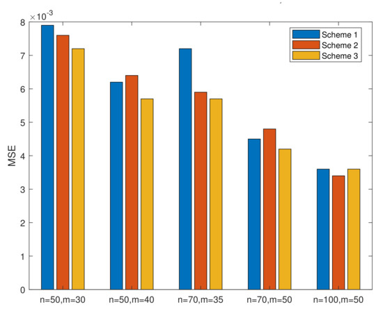Figure 2. MSEs of $C_{L_X}$ in Table 1 when k = 2.

(2)

From Table 2, we conclude that, in Bayesian estimation, the MSEs of $\alpha$, $\beta$, and $C_{L_X}$ decrease when we assume that m or n increases and that the k is invariant. When m and n are invariant, the MSEs of $\alpha$ increase while the MSEs of $\beta$ and $C_{L_X}$ decrease as k increases. From Table 2, Table 3, Table 4, Table 5, Table 6 and Table 7, the Bayesian estimation results based on the Lindley method perform better than the Bayesian estimation based on Metropolis–Hastings method in respect of MSEs. From Table 3 and Table 4, the result of Lindley approximation under LF when $\psi =1$ performs better than when $\psi =-1$. From Table 5 and Table 6, the result of Lindley approximation under GELF when $\phi =-1$ performs better than when $\phi =1$. It is also concluded from Table 1, Table 2, Table 3, Table 4, Table 5, Table 6 and Table 7 that the point estimation performs better as the failure proportion $\frac{m}{n}$ increases when k is invariant.

(3)

In Table 8, when we set that only one of the three parameters (k, m, and n) increases and the other two are invariant, the average length (AL) of 95% asymptotic confidence/HPD credible intervals narrow down. In almost all cases, the CP of $C_{L_X}$ reaches their prescribed confidence intervals. To conclude, it is better to apply the log-transformed MLEs than MLEs when considering the asymptotic confidence intervals.

Broadly speaking, the Bayesian estimation of parameters and the lifetime performance index is recommended in this situation.

7. Real Data Analysis

To illustrate the reliability of the simulation results using the methods discussed above, a set of real data is used here. We consider a lifetime data of 100 observations of tensile strength of carbon fibers. Reference [29] originally reported this data set which was later discussed by Reference [30]. The dataset is presented in Table 9.

Table 9. Real data set of breaking stress of carbon fibers (GPa).

3.70	3.11	4.42	3.28	3.75	2.96	3.39	3.31	3.15	2.81	1.41	2.76	3.19	1.59	2.17	3.51
1.84	1.61	1.57	1.89	2.74	3.27	2.41	3.09	2.43	2.53	2.81	3.31	2.35	2.77	2.68	4.91
1.57	2.00	1.17	2.17	0.39	2.79	1.08	2.88	2.73	2.87	3.19	1.87	2.95	2.67	4.20	2.85
2.55	2.17	2.97	3.68	0.81	1.22	5.08	1.69	3.68	4.70	2.03	2.82	2.50	1.47	3.22	3.15
2.97	2.93	3.33	2.56	2.59	2.83	1.36	1.84	5.56	1.12	2.48	1.25	2.48	2.03	1.61	2.05
3.60	3.11	1.69	4.90	3.39	3.22	2.55	3.56	2.38	1.92	0.98	1.59	1.73	1.71	1.18	4.38
0.85	1.80	2.12	3.65

In the first step, the complete data set is used for the log-logistic distribution fitting and the fitting results are compared to that of some well-informed distributions, for instance, Rayleigh distribution, inverse Weibull distribution, and generalized inverted exponential distribution (GIED). The probability density functions are $f(x)=\frac{2}{\theta }{e}^{-x^2/\theta }$, $f(x)=\alpha \beta x^{-(\alpha +1)}{e}^{-\beta x^{-\alpha }}$, and $f(x)=\frac{\alpha \beta }{x^2}{e}^{-\beta /x}{(1-e^{-\beta /x})}^{\alpha -1}$, respectively.

Based on the MLE method, various methods can be applied to test the fitting performance of the abovementioned distributions. We consider various indicators, $-lnL$, $AIC$, $BIC$, and Kolmogorov–Smirnov K-S statistics with p-value. $-lnL$ is estimated to be a negative log-likelihood function. $AIC(=2\times (p-lnL))$ is the Akaike information criterion. $BIC(=p\times ln(n)-2\times log(L))$ is Bayesian information criterion, where p is the parameter value of distribution, n is sample size, and L is the maximum of $lf$. If log-logistic distribution fits the data well, it will have the lowest statistic values of $-lnL$, $AIC$, $BIC$, and K-S and the highest statistic value of p-value. A graphical method in R is used to show the goodness of fitness of different distributions mentioned above. Quantile-quantile plots (Q-Q) are drawn and are showed in Figure 3. In Table 10, the values of MLEs of parameters, $-lnL$, $AIC$, $BIC$, and K-S statistics with p-value of different distributions are shown, and it is obvious that the log-logistic distribution best fits the lifetime data. Simultaneously, the above conclusions are clearly shown in Figure 3.

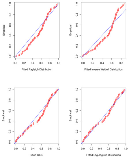
Figure 3. Q-Q plots.

Table 10. Fitting result.

Distribution	MLEs	-lnL	AIC	BIC	K-S	p-Value
Rayleigh	$\widehat{\theta }=7.8258$	149.0086	300.0172	302.6224	0.1402	0.039263
Inverse Weibull	$\widehat{\alpha }=1.7738$	172.4966	348.9931	354.2035	0.1761	0.004038
	$\widehat{\beta }=3.0856$
GIED	$\widehat{\alpha }=9.1967$	150.4161	304.8322	310.0426	0.1330	0.058198
	$\widehat{\beta }=6.2141$
Log-logistic	$\widehat{\alpha }=2.490$	145.3980	294.7960	300.0064	0.0860	0.449972
	$\widehat{\beta }=4.1455$

Next, randomly grouping the given data into $n=50$ groups with $k=2$ items in each, we obtain the progressive first-failure-censored sample in Table 11.

Table 11. Progressive first-failure-censored data of breaking stress of carbon fibers (GPa).

0.39	0.81	0.85	0.98	1.08	1.12	1.17	1.18	1.25	1.36	1.41	1.47	1.57	1.57	1.59	1.59
1.61	1.69	1.69	1.71	1.73	1.80	1.84	1.84	1.89	1.92	2.00	2.03	2.05	2.17	2.35	2.41
2.48	2.50	2.53	2.55	2.59	2.74	2.82	2.88	2.95	2.97	2.97	3.19	3.19	3.27	3.28	3.31
3.60	3.75

Then, for the abovementioned progressive first-failure censored data, three different censoring schemes when set at $m=30$ is applied to obtain three different censored samples. The first column in each row of Table 12 is a censored scheme, and the second column is the corresponding censored sample. We calculate the MLE and Bayes estimates of $\alpha$, $\beta$, and $C_{L_X}$ for three censoring schemes. For the Metropolis–Hastings procedure, we take $M=1000$. We also obtain 95% asymptotic confidence and HPD credible intervals for $\alpha$ and $\beta$. The results are listed in Table 13.

Table 12. The MLEs and Bayes estimates of $\alpha$, $\beta$, and $C_{L_X}$ of a real data set.

Censoring Scheme	${\mathfrak{R}}_{\mathfrak{1}}$	${\mathfrak{R}}_{\mathfrak{2}}$	${\mathfrak{R}}_{\mathfrak{3}}$
${\widehat{\alpha }}_{ML}$	3.0026 ( 2.7037,3.3014)	2.8616 (2.4917,3.2315)	2.5402 (2.1406,2.9398)
${\widehat{\beta }}_{ML}$	5.1557 (3.6353,6.6761)	3.9363 (2.7578,5.1148)	3.3795 (2.31100,4.4480)
${\widehat{C_{L_X}}}_{ML}$	1.8021	1.2854	0.9945
${\widehat{\alpha }}_{-SELF}$	3.0241	2.9038	2.5987
${\widehat{\beta }}_{-SELF}$	5.0412	3.8403	3.2878
${\widehat{C_{L_X}}}_{-SELF}$	2.3527	1.5038	1.1405
${\widehat{\alpha }}_{MH}$	2.9774 (2.1088,3.1307)	2.9453 (2.1960,3.1280)	2.4499 (2.0829,2.6401)
${\widehat{\beta }}_{MH}$	4.6815 (3.6730,5.7100)	3.6493 (3.1578,4.9303)	3.7345 (3.2811,4.5882)
${\widehat{C_{L_X}}}_{MH}$	1.6024	1.1778	1.1097

Table 13. Different progressive first-failure censored samples of various censored scheme when $k=2,n=50,$ and $m=30$.

Censoring Scheme	Sample
${\mathfrak{R}}_{\mathfrak{1}}=(20,(0*29))$	0.39, 1.80, 1.84, 1.84, 1.89, 1.92, 2.00, 2.03, 2.05, 2.17, 2.35, 2.41, 2.48, 2.50, 2.53, 2.55, 2.59, 2.74
	2.82, 2.88, 2.95, 2.97, 2.97, 3.19, 3.19, 3.27, 3.28, 3.31, 3.60, 3.75
${\mathfrak{R}}_{\mathfrak{2}}=(10,(0*28),10)$	0.39, 1.47, 1.57, 1.57, 1.59, 1.59, 1.61, 1.69, 1.69, 1.71, 1.73, 1.80, 1.84, 1.84, 1.89, 1.92, 2.00, 2.03
	2.05, 2.17, 2.35, 2.41, 2.48, 2.50, 2.53, 2.55, 2.59, 2.74, 2.82, 2.88
${\mathfrak{R}}_{\mathfrak{3}}=((0*29),20)$	0.39, 0.81, 0.85, 0.98, 1.08, 1.12, 1.17, 1.18, 1.25, 1.36, 1.41, 1.47, 1.57, 1.57, 1.59, 1.59, 1.61, 1.69
	1.69, 1.71, 1.73, 1.80, 1.84, 1.84, 1.89, 1.92, 2.00, 2.03, 2.05, 2.17

8. Optimal Censoring Plan

The point and interval estimation of unknown quantities $\alpha$ and $\beta$ and the lifetime performance index $C_{L_X}$ of log-logistic distribution is analysed with progressive first-failure censored data. In simulation and real data analysis, different censoring schemes have been considered. It raises the problem about how to decide the optimal censoring schemes. Many scholars and researchers—see [7,31]—have studied the criteria of comparing and analyzing different progressive and hybrid censored schemes. It is desirable in life-testing experiments to select the optimal censoring schemes from a set of censoring schemes as well as in reliability theory. Here are some evaluation criteria that we consider:

Criterion 1:

$\mathbf{Minimum}\mathbf{determinant}\mathbf{of}{\mathbf{I}}^{-\mathbf{1}}$$(\widehat{\theta })$. Under this criterion, the optimal censoring scheme for the experiment is supposed to have the minimum value of the determinant of $I^{-1}(\widehat{\theta })$ of MLEs.

Criterion 2:

$\mathbf{Minimum}\mathbf{trace}{\mathbf{I}}^{-\mathbf{1}}$$(\widehat{\theta })$. The optimal censoring scheme is considered to have the minimum value of the trace of $I^{-1}(\widehat{\theta })$ of MLEs under this criterion. Without scale-invariant characteristic, criteria 1 and 2 are efficacious when lifetime distributions have one parameter.

Criterion 3:

$\mathbf{Minimum}\mathbf{Var}[ln{\widehat{\mathbf{T}}}_{\mathbf{p}}]$. Under this criterion, the optimal censoring scheme has the minimum value of $(ln{\widehat{T}}_p)$ and the pth $(0<p<1)$ quantile of the MLE logarithmic variance of log-logistic distribution can also be written as $ln{T}_p=ln\left[\alpha {(\frac{p}{1-p})}^{1/\beta }\right]$. We can get the approximation value of $Var(ln{\widehat{T}}_p)$ as ${[\nabla ln{\widehat{T}}_p]}^T\left[Var(\widehat{\theta })\right][\nabla ln{\widehat{T}}_p]$, where ${[\nabla ln{\widehat{T}}_p]}^T={(\frac{\partial \nabla ln{T}_p}{\partial \alpha },\frac{\partial \nabla ln{T}_p}{\partial \beta })}_{\alpha =\widehat{\alpha },\beta =\widehat{\beta }}$. The results of criterion 3 hinges on the selection of p.

Criterion 4:

$\mathbf{Minimum}{\int }_{\mathbf{0}}^{\mathbf{1}}\mathbf{Var}\left[\mathbf{ln}{\widehat{\mathbf{T}}}_{\mathbf{p}}\right]\mathbf{w}(\mathbf{p})\mathbf{d}\mathit{p}$. $ln{\widehat{T}}_p$ is defined in criterion 3. $w(p)$ is nonnegative and satisfies ${\int }_0^{1}w(p)dp=1$. We take $w(p)=1$ when $0<p<1$.

$\mathsf{Example}$: Based on the real data set analyzed in Section 7, we elaborate on how the above criteria are utilized in actual tests. p = 0.05 and p = 0.95 are two different values computed under criterion 3. The values that we calculated are shown in Table 14. Conclusions are that ${\mathfrak{R}}_{\mathfrak{1}}$ is the optimal scheme under criteria 3 and 4, and ${\mathfrak{R}}_{\mathfrak{3}}$ is optimal for criteria 1 and 2.

Table 14. Comparison of censoring schemes when $k=2,n=50,$ and $m=30$.

Censoring Scheme			Criterion
	det$({\mathbf{I}}^{-\mathbf{1}}(\widehat{\mathbf{\theta }}))$	trace$({\mathbf{I}}^{-\mathbf{1}}(\widehat{\mathbf{\theta }}))$	$\mathbf{Var}[ln{\widehat{\mathbf{T}}}_{\mathbf{0.05}}]$	$\mathbf{Var}[ln{\widehat{\mathbf{T}}}_{\mathbf{0.95}}]$	${\int }_{\mathbf{0}}^{\mathbf{1}}\mathbf{Var}[ln{\widehat{\mathbf{T}}}_{\mathbf{p}}]\mathbf{dp}$
${\mathfrak{R}}_{\mathfrak{1}}=(20,(0*29))$	0.0130	0.6250	$\mathbf{0.0238}$	$\mathbf{0.0320}$	$\mathbf{0.0266}$
${\mathfrak{R}}_{\mathfrak{2}}=(10,(0*28),10)$	0.0102	0.3972	0.0259	0.0428	0.0317
${\mathfrak{R}}_{\mathfrak{3}}=((0*29),20)$	$\mathbf{0.0080}$	$\mathbf{0.3388}$	0.0303	0.0611	0.0407

9. Conclusions

Our main consideration is the lifetime performance index $C_L$, an indicator employed to evaluate the performance of a progress. In this article, different methods of estimating $C_L$ with progressive first-failure-censored data with the log-logistic distribution is discussed carefully. Both the MLE and the Bayesian estimation of $\alpha$ and $\beta$ and the lifetime performance index $C_L$ are investigated. The main difference between MLE and the Bayes estimate is the consideration of prior distributions. The parameters are regarded as unknown variables in MLE while they are random variables following known prior distributions in Bayesian estimation. For Bayesian estimation, Lindley method and the Monte Carlo Markov Chain method are applyed to approximate the Bayes estimator under asymmetric and symmetric loss functions. Asymptotic confidence intervals are constructed based on MLEs and log-transformed MLEs applying the observed Fisher information matrix. The HPD confidence intervals are studied applying the Metropolis–Hastings algorithm with the type of random walk chain. The performances of estimations have been compared and discussed. Also, four criteria of selecting optimal censoring plan in a real life test have been considered since it is significant for a researcher to determine under certain circumstances which censoring scheme will best fit the life-testing experiment.

It is worth noting that, here, we focus on the functional time of a product, which is strongly related to manufacturers and designers and can be enhanced on aspects of innovation, technology, design improvement, and systems approaches. Refurbishment, remanufacturing, and various business models can extend product life cycles since products can have one or more use. In this way, materials can be recycled into other products so that we can better defend the environment. For more detailed information, see References [32,33].

Appendix C.1. The Squared Error Loss Function

$$\begin{array}{cc}\hfill {\varphi }_1& =\frac{L_X}{{\alpha }^2\sqrt{\frac{2\pi csc\left(\frac{2\pi }{\beta }\right)}{\beta }-\frac{{\pi }^2{csc}^2\left(\frac{\pi }{\beta }\right)}{{\beta }^2}}},\hfill \\ \hfill {\varphi }_2& =\mathbb{M}-C_{L_X}\mathbb{N}\hfill \\ \hfill {\varphi }_{11}& =-\frac{2L_X}{{\alpha }^3\sqrt{\frac{2\pi csc\left(\frac{2\pi }{\beta }\right)}{\beta }-\frac{{\pi }^2{csc}^2\left(\frac{\pi }{\beta }\right)}{{\beta }^2}}},\hfill \\ \hfill {\varphi }_{12}& ={\varphi }_{21}=-\frac{L_X\mathbb{N}}{{\alpha }^2\sqrt{\frac{2\pi csc\left(\frac{2\pi }{\beta }\right)}{\beta }-\frac{{\pi }^2{csc}^2\left(\frac{\pi }{\beta }\right)}{{\beta }^2}}},\hfill \\ \hfill {\varphi }_{22}& =\mathbb{R}-2\mathbb{M}\mathbb{N}+3C_{L_X}{\mathbb{N}}^2-\frac{\mathbb{S}{C}_{L_X}}{2\left(\frac{2\pi csc\left(\frac{2\pi }{\beta }\right)}{\beta }-\frac{{\pi }^2{csc}^2\left(\frac{\pi }{\beta }\right)}{{\beta }^2}\right)}.\hfill \end{array}$$

where

$$\begin{array}{cc}\hfill \mathbb{S}=& -\frac{2{\pi }^4{csc}^4\left(\frac{\pi }{\beta }\right)}{{\beta }^6}+\frac{12{\pi }^{3}cot\left(\frac{\pi }{\beta }\right){csc}^2\left(\frac{\pi }{\beta }\right)}{{\beta }^5}-\frac{6{\pi }^2{csc}^2\left(\frac{\pi }{\beta }\right)}{{\beta }^4}-\frac{4{\pi }^4{cot}^2\left(\frac{\pi }{\beta }\right){csc}^2\left(\frac{\pi }{\beta }\right)}{{\beta }^6}\hfill \\ & +\frac{8{\pi }^3{csc}^3\left(\frac{2\pi }{\beta }\right)}{{\beta }^5}+\frac{8{\pi }^3{cot}^2\left(\frac{2\pi }{\beta }\right)csc\left(\frac{2\pi }{\beta }\right)}{{\beta }^5}+\frac{4\pi csc\left(\frac{2\pi }{\beta }\right)}{{\beta }^3}-\frac{16{\pi }^{2}cot\left(\frac{2\pi }{\beta }\right)csc\left(\frac{2\pi }{\beta }\right)}{{\beta }^4}\hfill \\ \hfill \mathbb{R}=& \frac{\frac{{\pi }^3{csc}^3\left(\frac{\pi }{\beta }\right)}{{\beta }^5}+\frac{{\pi }^3{cot}^2\left(\frac{\pi }{\beta }\right)csc\left(\frac{\pi }{\beta }\right)}{{\beta }^5}-\frac{4{\pi }^{2}cot\left(\frac{\pi }{\beta }\right)csc\left(\frac{\pi }{\beta }\right)}{{\beta }^4}+\frac{2\pi csc\left(\frac{\pi }{\beta }\right)}{{\beta }^3}}{\sqrt{\frac{2\pi csc\left(\frac{2\pi }{\beta }\right)}{\beta }-\frac{{\pi }^2{csc}^2\left(\frac{\pi }{\beta }\right)}{{\beta }^2}}}\hfill \end{array}$$

(A1)

Appendix C.2. The Linex Loss Function

$$\begin{array}{cc}\hfill {\varphi }_1& =-\psi e^{-\psi C_{L_X}}\frac{L_X}{{\alpha }^2\sqrt{\frac{2\pi csc\left(\frac{2\pi }{\beta }\right)}{\beta }-\frac{{\pi }^2{csc}^2\left(\frac{\pi }{\beta }\right)}{{\beta }^2}}},\hfill \\ \hfill {\varphi }_{11}& ={\psi }^2{e}^{-\psi C_{L_X}}\frac{L_X^2}{{\alpha }^4\left[\frac{2\pi csc\left(\frac{2\pi }{\beta }\right)}{\beta }-\frac{{\pi }^2{csc}^2\left(\frac{\pi }{\beta }\right)}{{\beta }^2}\right]}+\psi e^{-\psi C_{L_X}}\frac{2L_X}{{\alpha }^3\sqrt{\frac{2\pi csc\left(\frac{2\pi }{\beta }\right)}{\beta }-\frac{{\pi }^2{csc}^2\left(\frac{\pi }{\beta }\right)}{{\beta }^2}}},\hfill \\ \hfill {\varphi }_{12}={\varphi }_{21}& =\frac{e^{-\psi C_{L_X}}\psi L_X\mathbb{N}}{{\alpha }^2\sqrt{\frac{2\pi csc\left(\frac{2\pi }{\beta }\right)}{\beta }-\frac{{\pi }^2{csc}^2\left(\frac{\pi }{\beta }\right)}{{\beta }^2}}}+\frac{L_X\psi e^{-\psi C_{L_X}}}{{\alpha }^2\sqrt{\frac{2\pi csc\left(\frac{2\pi }{\beta }\right)}{\beta }-\frac{{\pi }^2{csc}^2\left(\frac{\pi }{\beta }\right)}{{\beta }^2}}}\left[-\psi \mathbb{M}+\psi C_{L_X}\mathbb{N}\right],\hfill \end{array}$$

$$\begin{array}{cc}\hfill {\varphi }_2=& e^{-\psi C_{L_X}}\left[-\psi \mathbb{M}+\psi C_{L_X}\mathbb{N}\right]\hfill \\ \hfill {\varphi }_{22}=& e^{-\psi C_{L_X}}{\left[-\psi \mathbb{M}+\psi C_{L_X}\mathbb{N}\right]}^2+e^{-\psi C_{L_X}}\left[-\psi \mathbb{R}+2\psi \mathbb{M}\mathbb{N}-3\psi C_{L_X}{\mathbb{N}}^2+\frac{\psi C_{L_X}\mathbb{S}}{2\left(\frac{2\pi csc\left(\frac{2\pi }{\beta }\right)}{\beta }-\frac{{\pi }^2{csc}^2\left(\frac{\pi }{\beta }\right)}{{\beta }^2}\right)}\right]\hfill \end{array}$$

(A2)

Appendix C.3. The General Entropy Loss Function

$$\begin{array}{cc}\hfill {\varphi }_1=& -\frac{L\phi C_{L_X}^{-\phi -1}}{{\alpha }^2\sqrt{\frac{2\pi csc\left(\frac{2\pi }{\beta }\right)}{\beta }-\frac{{\pi }^2{csc}^2\left(\frac{\pi }{\beta }\right)}{{\beta }^2}}},\hfill \\ \hfill {\varphi }_{11}=& \frac{2L\phi C_{L_X}^{-\phi -1}}{{\alpha }^3\sqrt{\frac{2\pi csc\left(\frac{2\pi }{\beta }\right)}{\beta }-\frac{{\pi }^2{csc}^2\left(\frac{\pi }{\beta }\right)}{{\beta }^2}}}+{\displaystyle \frac{L^2(\phi +1)\phi C_{L_X}^{-\phi -2}}{{\alpha }^4\left(\frac{2\pi csc\left(\frac{2\pi }{\beta }\right)}{\beta }-\frac{{\pi }^2{csc}^2\left(\frac{\pi }{\beta }\right)}{{\beta }^2}\right)}},\hfill \\ \hfill {\varphi }_{12}={\varphi }_{21}=& \frac{L\phi \mathbb{N}{C}_{L_X}^{-\phi -1}}{{\alpha }^2\sqrt{\frac{2\pi csc\left(\frac{2\pi }{\beta }\right)}{\beta }-\frac{{\pi }^2{csc}^2\left(\frac{\pi }{\beta }\right)}{{\beta }^2}}}+\frac{L(\phi +1)\phi C_{L_X}^{-\phi -2}}{{\alpha }^2\sqrt{\frac{2\pi csc\left(\frac{2\pi }{\beta }\right)}{\beta }-\frac{{\pi }^2{csc}^2\left(\frac{\pi }{\beta }\right)}{{\beta }^2}}}\times (\mathbb{M}-C_{L_X}\mathbb{N})\hfill \\ \hfill {\varphi }_2=& -\phi C_{L_X}^{-\phi -1}(\mathbb{M}-C_{L_X}\mathbb{N}),\hfill \\ \hfill {\varphi }_{22}=& (\phi +1)\phi C_{L_X}^{-\phi -2}{\left(\mathbb{M}-C_{L_X}\mathbb{N}\right)}^2-\phi C_{L_X}^{-\phi -1}\left(\mathbb{R}-2\mathbb{M}\mathbb{N}+3C_{L_X}{\mathbb{N}}^2\right.\hfill \\ & -\left.\frac{C_{L_X}\mathbb{S}}{2\left(\frac{2\pi csc\left(\frac{2\pi }{\beta }\right)}{\beta }-\frac{{\pi }^2{csc}^2\left(\frac{\pi }{\beta }\right)}{{\beta }^2}\right)}\right).\hfill \end{array}$$

References

- Cooper, T. Longer Lasting Products: Alternatives to the Throwaway Society; CRC Press: Boca Raton, FL, USA, 2016. [Google Scholar]
- Ertz, M.; Leblanc-Proulx, S.; Sarigllü, E.; Morin, V. Advancing quantitative rigor in the circular economy literature: New methodology for product lifetime extension business models. Resour. Conserv. Recycl. 2019, 150, 1–12. [Google Scholar] [CrossRef]
- Montgomery, D.C. Introduction to Statistical Quality Control; John Wiley & Sons: Hoboken, NJ, USA, 1991. [Google Scholar]
- Wu, J.W.; Lee, H.M.; Lei, C.L. Computational testing algorithmic procedure of assessment for lifetime performance index of products with two-parameter exponential distribution. Appl. Math. Comput. 2007, 190, 116–125. [Google Scholar] [CrossRef]
- Lee, W.C.; Wu, J.W.; Hong, C.W. Assessing the Lifetime Performance Index of Products with the Exponential Distribution under Progressively Type II Right Censored Samples; Elsevier Science: Amsterdam, The Netherlands, 2009. [Google Scholar]
- Lee, H.M.; Wu, J.W.; Lei, C.L.; Hung, W.L. Implementing lifetime performance index of products with two-parameter exponential distribution. Int. J. Syst. Sci. 2011, 42, 1305–1321. [Google Scholar] [CrossRef]
- Sultan, K.; Alsadat, N.; Kundu, D. Bayesian and maximum likelihood estimations of the inverse Weibull parameters under progressive type-II censoring. J. Stat. Comput. Simul. 2014, 84, 2248–2265. [Google Scholar] [CrossRef]
- Lee, K.; Cho, Y. Bayesian and maximum likelihood estimations of the inverted exponentiated half logistic distribution under progressive Type II censoring. J. Appl. Stat. 2016, 44, 811–832. [Google Scholar] [CrossRef]
- Cohen, A.C. Progressively Censored Samples in Life Testing. Technometrics 1963, 5, 327–339. [Google Scholar] [CrossRef]
- Mohammed, H.S. Statistical inferences based on an adaptive progressive type-II censoring from exponentiated exponential distribution. J. Egypt. Math. Soc. 2017, 25, 393–399. [Google Scholar]
- Balakrishnan, N.; Aggarwala, R. Progressive Censoring: Theory, Methods, and Applications; Birkhäuser: Boston, MA, USA, 2000. [Google Scholar]
- Johnson, L.G. Theory And Technique Of Variation Research; Elsevier Pub. Co.: Amsterdam, The Netherlands, 1964. [Google Scholar]
- Wu, S.J.; Kuş, C. On estimation based on progressive first-failure-censored sampling. Comput. Stat. Data Anal. 2009, 53, 3659–3670. [Google Scholar] [CrossRef]
- Ahmed, E.A. Estimation and prediction for the generalized inverted exponential distribution based on progressively first-failure-censored data with application. J. Appl. Stat. 2017, 44, 1576–1608. [Google Scholar] [CrossRef]
- Madhulika, D.; Renu, G.; Hare, K. On progressively first failure censored Lindley distribution. Comput. Stat. 2016, 31, 139–163. [Google Scholar]
- Soliman, A.A.; Abd-Ellah, A.H.; Abou-Elheggag, N.A.; Abd-Elmougod, G.A. Estimation of the parameters of life for Gompertz distribution using progressive first-failure censored data. Comput. Stat. Data Anal. 2012, 56, 2471–2485. [Google Scholar] [CrossRef]
- Ahmadi, M.V.; Doostparast, M.; Ahmadi, J. Estimating the lifetime performance index with Weibull distribution based on progressive first-failure censoring scheme. J. Comput. Appl. Math. 2013, 239, 93–102. [Google Scholar] [CrossRef]
- Madhulika, D.; Hare, K.; Renu, G. Generalized inverted exponential distribution under progressive first-failure censoring. J. Stat. Comput. Simul. 2016, 86, 1095–1114. [Google Scholar]
- Ahmed, A.; Soliman, M.M.A.S. Bayesian MCMC inference for the Gompertz distribution based on progressive first-failure censoring data. AIP Conf. Proc. 2015, 1643, 125–134. [Google Scholar]
- Ahmadi, M.V.; Doostparast, M. Pareto analysis for the lifetime performance index of products on the basis of progressively first-failure-censored batches under balanced symmetric and asymmetric loss functions. J. Appl. Stat. 2019, 46, 1196–1227. [Google Scholar] [CrossRef]
- Akhtar, M.T.; Khan, A.A.; Akhtar, M.T.; Khan, A.A. Log-logistic Distribution as a Reliability Model: A Bayesian Analysis. Am. J. Math. Stat. 2014, 4, 162–170. [Google Scholar]
- Al-Shomrani, A.A.; Shawky, A.I.; Arif, O.H.; Aslam, M. Log-logistic distribution for survival data analysis using MCMC. Springerplus 2016, 5, 1774. [Google Scholar] [CrossRef]
- Lesitha, G.P.Y.T. Estimation of the scale parameter of a log-logistic distribution. Metrika 2013, 76, 427–448. [Google Scholar] [CrossRef]
- William, Q.; Meeker; Luis, A. Escobar Statistical Methods for Reliability Data. Technometrics 1998, 40, 254–256. [Google Scholar]
- Lindley, D.V. Approximate Bayesian methods. Trab. Estad. Y Investig. Oper. 1980, 31, 223–245. [Google Scholar] [CrossRef]
- Nassar, M.; Abo-Kasem, O.; Zhang, C.; Dey, S. Analysis of Weibull Distribution Under Adaptive Type-II Progressive Hybrid Censoring Scheme. J. Ind. Soc. Probab. Stat. 2018, 19, 25–65. [Google Scholar] [CrossRef]
- Albert, J.; Chopin, N. Bayesian computation with R. Stat. Comput. 2009, 19, 111–112. [Google Scholar]
- Balakrishnan, N.; Sandhu, R.A. A Simple Simulational Algorithm for Generating Progressive Type-II Censored Samples. Am. Stat. 1995, 49, 229–230. [Google Scholar]
- Nichols, M.D.; Padgett, W.J. A Bootstrap Control Chart for Weibull Percentiles. Qual. Reliab. Eng. 2006, 22, 141–151. [Google Scholar] [CrossRef]
- Mohammed, H.S.; Ateya, S.F.; AL-Hussaini, E.K. Estimation based on progressive first-failure censoring from exponentiated exponential distribution. J. Appl. Stat. 2017, 44, 1479–1494. [Google Scholar] [CrossRef]
- Pradhan, B.; Kundu, D. On progressively censored generalized exponential distribution. Test 2009, 18, 497–515. [Google Scholar] [CrossRef]
- Den Hollander, M.C.; Bakker, C.A.; Hultink, E.J. Product Design in a Circular Economy: Development of a Typology of Key Concepts and Terms. J. Ind. Ecol. 2017, 21, 517–525. [Google Scholar] [CrossRef]
- Ertz, M.; Leblanc-Proulx, S.; Sarigollu, E.; Morin, V. Made to break? A taxonomy of business models on product lifetime extension. J. Clean. Prod. 2019, 234, 867–880. [Google Scholar] [CrossRef]
© 2020 by the authors. Licensee MDPI, Basel, Switzerland. This article is an open access article distributed under the terms and conditions of the Creative Commons Attribution (CC BY) license (http://creativecommons.org/licenses/by/4.0/).