Cosmological Solutions for the Geometrical Scalar-Tensor with the Potential Determined by the Noether Symmetry Approach

Abstract

The aim of this work is to study a scalar-tensor theory where owing to Palatini’s variational method the space-time is endowed with a geometrical structure of Weyl integrable type. The geometrical nature of the scalar field is related to the non-metricity so that the theory is known as geometrical scalar-tensor. On the framework of Weyl transformations, a non-minimally coupled scalar-tensor theory on the Jordan frame corresponds to a minimally coupled Einstein–Hilbert action on the Einstein frame. The scalar potential is selected by the Noether symmetry approach in order to obtain conserved quantities for the FRW cosmological model. Exact solutions are obtained and analyzed in the context of the cosmological scenarios consistent with an expanding universe. A particular case is matched in each frame and the role of scalar field as a dark energy component is discussed.

1. Introduction

Although Einstein’s theory of gravity is constantly being supported by current observational data [1], recent issues such as the accelerated expansion of the Universe and the possible existence of dark matter, can not be fully explained only based on general relativity. In this sense, there have been considerable efforts in the development of alternative theories to Einstein’s theory [2]. In particular, there is a great interest in investigating new possibilities that include changes in the theory of general relativity [3,4].

Scalar-tensor (ST) theories are among the proposed extensions of Einstein’s theory [5,6,7,8]. A geometrical approach to theories with non-minimal coupling is particularly interesting. According to it, by considering the Palatini variational method a not necessarily Riemannian compatibility condition between the metric tensor and the affine connection—initially taken as independent variables—is obtained [9,10]. Furthermore, it was shown that the geometry that naturally appears when a symmetric affine connection is regarded is the so called integrable Weyl geometry, where the scalar field takes part together with the metric tensor in the description of the gravitational field. This brings a geometrical origin for the scalar field present in the theory, which naturally define the known as geometrical scalar-tensor theories [11,12].

The potential term is obtained through the Noether symmetry approach, which allows making a choice that leads to a quantity conserved in the model [13,14,15,16]. Such a conserved quantity will imply the existence of a cyclic variable useful to find exact solutions for the field equation. This approach has already been used in choosing for models of tensor-scalar theories that could describe the dynamics of the expanding universe, as dark energy models [17,18,19,20].

In the organization of this work the action of the model is presented in Section 2. In Section 3 the field equations for a spatially flat Friedmann–Robertson–Walker (FRW) are obtained from a point-like Lagrangian. Noether symmetry approach is considered in the Section 4 to specify the self-interacting potential of the scalar field. In Section 5 the field equations are integrated and the cosmological solutions in each frame are fulfilled in the Section 6. The particular case $\omega =1/2$ is seen in Section 7. The paper is closed with the conclusions in Section 8.

We will adopt natural units, such that $8\pi G=\hslash =c=1$. Besides that, we will take the metric signature $(+,-,-,-)$.

2. The Model and the Weyl Transformations

A well-known scalar-tensor theory called dilaton gravity can be expressed through the following action

$${\mathcal{S}}_{JF}=\int d^{4}x\sqrt{-g}{e}^{-\varphi }\left[R+\omega {\varphi }^{,\alpha }{\varphi }_{,\alpha }-e^{-\varphi }V\left(\varphi \right)\right],$$

(1)

where $\varphi$ represents a scalar field, $V\left(\varphi \right)$ its self-interacting potential and $\omega$ a dimensionless coupling constant. Furthermore, R is the Ricci scalar, calculated with the affine connection ${\Gamma }_{\mu \nu }^{\alpha }$. We have represented ${\mathcal{S}}_{JF}$ to write the Action on the Jordan frame.

When Palatini variation is used in non-minimally coupled scalar-tensor theories, as this one, the affine connection is not the same of the Levi–Civita connection, expressed in terms of the Christoffel symbols. This is the main difference that arises between the Palatini variation method and the said metric variation. Considering the affine connection and the metric tensor as independent variables in the action extremization, the variation with respect to connection yields a relation between affine connection and the metric tensor that can be written as

$${\nabla }_{\alpha }{g}_{\mu \nu }={\varphi }_{,\alpha }{g}_{\mu \nu }$$

(2)

widely used in the literature that studies the so-called integrable Weyl manifolds, or non-metricity geometries [21,22]. That is, as a consequence of Palatini variation, the geometric structure of space-time, manifested through the affine connection, is given dynamically by the action, instead of being imposed a priori, as in the case of metric variation. So, the theory is called a geometrical scalar-tensor, because the scalar field has a geometric origin, related to the non-metricity of the manifold.

It is easy to see, after some algebraic manipulations of Equation (2) that the affine connection takes the following form

$${\Gamma }_{\mu \nu }^{\alpha }={\{}_{\mu \nu }^{\alpha }\}-\frac{1}{2}{g}^{\alpha \beta }\left(g_{\mu \beta }{\varphi }_{,\nu }+g_{\nu \beta }{\varphi }_{,\mu }-g_{\mu \nu }{\varphi }_{,\beta }\right),$$

(3)

where ${\{}_{\mu \nu }^{\alpha }\}=\frac{1}{2}{g}^{\alpha \beta }\left({\partial }_{\nu }{g}_{\mu \beta }+{\partial }_{\mu }{g}_{\nu \beta }-{\partial }_{\beta }{g}_{\mu \nu }\right)$ represent the Christoffel symbols. Both Equations (2) and (3) are invariant by Weyl transformations

$$\begin{array}{c}{\overline{g}}_{\mu \nu }=e^f{g}_{\mu \nu }\end{array}$$

(4)

$$\begin{array}{c}\overline{\varphi }=\varphi +f\end{array}$$

(5)

where f is a arbitrary scalar function, or a gauge. It is possible choose a f that leads Equation (1) to the Einstein frame

$${\mathcal{S}}_{EF}=\int d^{4}x\sqrt{-\overline{g}}\left[\overline{R}+\omega {\varphi }^{,\alpha }{\varphi }_{,\alpha }-V\left(\varphi \right)\right],$$

(6)

where $\overline{R}=e^{-\varphi }R$, because the Ricci tensor is invariant over Weyl transformations, but Ricci scalar is not. We have seen that the action Equation (1) corresponds the well-known action Equation (6) by Weyl transformations. Both theories are extensively studied in the literature, although the relationship between them is not so approached from the geometric point of view. In addition, both the scalar field and the scalar potential are entered by hand. In this work we are using the methods mentioned in the references to justify both the origin of the scalar field and the choice of the scalar potential.

Let us obtain the field equation by performing the variation with respect to $g_{\mu \nu }$

$$R_{\mu \nu }-\frac{1}{2}R{g}_{\mu \nu }=-T_{\mu \nu }^{\left(\varphi \right)}$$

(7)

where $T_{\mu \nu }^{\left(\varphi \right)}$ is the energy-momentum tensor of the scalar field

$$T_{\mu \nu }^{\left(\varphi \right)}=\omega \left({\partial }_{\mu }\varphi {\partial }_{\nu }\varphi -\frac{1}{2}{\varphi }^{,\alpha }{\varphi }_{,\alpha }{g}_{\mu \nu }\right)+\frac{1}{2}{e}^{-\varphi }V{g}_{\mu \nu }.$$

(8)

However, in order to identify the Einstein tensor calculated with the Christoffel symbols and to define an effective energy–momentum tensor gathering the scalar field terms, we need to express Equation (7) as follows

$${\tilde{R}}_{\mu \nu }-\frac{1}{2}\tilde{R}{g}_{\mu \nu }=-{\mathcal{T}}_{\mu \nu },$$

(9)

where ${\overline{R}}_{\mu \nu }$ and $\overline{R}$ are the usual Ricci tensor and Ricci scalar calculated with metric connection, and we have defined the effective energy–momentum tensor

$${\mathcal{T}}_{\mu \nu }\doteq T_{\mu \nu }^{\left(\varphi \right)}-{\tilde{\nabla }}_{\mu }{\varphi }_{,\nu }-\frac{1}{2}{\varphi }_{,\mu }{\varphi }_{,\nu }-g_{\mu \nu }\left(\frac{1}{4}{\varphi }_{,\alpha }{\varphi }^{,\alpha }-{\tilde{\nabla }}_{\alpha }{\varphi }^{,\alpha }\right),$$

(10)

which by using Equation (8) can be expressed simply as follows

$${\mathcal{T}}_{\mu \nu }\equiv \left(\omega -\frac{1}{2}\right){\varphi }_{,\mu }{\varphi }_{,\nu }-{\tilde{\nabla }}_{\mu }{\varphi }_{,\nu }-\frac{1}{2}{g}_{\mu \nu }\left[\left(\omega +\frac{1}{2}\right){\varphi }_{,\alpha }{\varphi }^{,\alpha }-e^{-\varphi }V-2{\tilde{\nabla }}_{\alpha }{\varphi }^{,\alpha }\right].$$

(11)

Furthermore, by performing the variation of the action with respect to the scalar field $\varphi$, we obtain the following field equation,

$$\tilde{\square }\varphi -{\varphi }^{,\alpha }{\varphi }_{,\alpha }+\frac{e^{-\varphi }}{2\omega }\frac{dV}{d\varphi }=0.$$

(12)

3. Pointlike Lagrangian and FRW and Klein-Gordon Equations

We are interested to analyze a homogeneous and isotropic universe described by the spatially flat Friedmann–Robertson–Walker metric

$$d{s}^2=d{t}^2-a^2\left(t\right)\left[d{x}^2+d{y}^2+d{z}^2\right].$$

(13)

Besides that, in order to not spoil the homogeneity and isotropicity, we require that $\varphi =\varphi \left(t\right)$. Therefore, according to the metric Equation (13) the kinetic term of the scalar field will reduce to

$$\omega g^{\mu \nu }{\varphi }_{,\mu }{\varphi }_{,\nu }=\omega {\dot{\varphi }}^2,$$

(14)

where dot means derivative with respect to coordinate t. In terms of the metric Equation (13) the Ricci scalar will be expressed by

$$R=6\left(\frac{\ddot{a}}{a}+\frac{{\dot{a}}^2}{a^2}\right)+\frac{3}{2}\left({\dot{\varphi }}^2-6\dot{\varphi }\frac{\dot{a}}{a}-2\ddot{\varphi }\right).$$

(15)

In this way, by using Equations (14) and (15) in Equation (1), and that $d^{4}x\sqrt{-g}=a^{3}dt{d}^{3}x$, we will have

$${\mathcal{S}}_{JF}={\mathcal{V}}_o\int dt{e}^{-\varphi }\left[6\left(a^2\ddot{a}+a{\dot{a}}^2\right)+\frac{3}{2}\left(a^3{\dot{\varphi }}^2-6a^2\dot{a}\dot{\varphi }-2a^3\ddot{\varphi }\right)+\omega a^3{\dot{\varphi }}^2-a^3{e}^{-\varphi }V\left(\varphi \right)\right],$$

(16)

where we have defined ${\mathcal{V}}_o$ as the 3-volume

$${\mathcal{V}}_o\doteq \underset{\mathcal{M}}{\int }{d}^{3}x.$$

(17)

The Equation (16) can be integrated by parts to separate terms of total derivative. Thus, by running this procedure we will get the following reduced action

$${\mathcal{S}}_{JF}=V_o\int dt\left\{e^{-\varphi }\left[\left(\omega -\frac{3}{2}\right)a^3{\dot{\varphi }}^2+6\left(a^2\dot{a}\dot{\varphi }-a{\dot{a}}^2\right)-a^3{e}^{-\varphi }V\left(\varphi \right)\right]+\frac{d}{dt}\left[e^{-\varphi }{a}^2\left(6\dot{a}-3a\dot{\varphi }\right)\right]\right\}.$$

(18)

Thus, after neglecting surface terms, we obtain the pointlike Lagrangian

$${\mathcal{L}}_{JF}\doteq e^{-\varphi }\left[\left(\omega -\frac{3}{2}\right)a^3{\dot{\varphi }}^2+6\left(a^2\dot{a}\dot{\varphi }-a{\dot{a}}^2\right)-a^3{e}^{-\varphi }V\left(\varphi \right)\right].$$

(19)

From the Euler–Lagrange equation for a applied to Equation (19),

$$\frac{d}{dt}\left(\frac{\partial \mathcal{L}}{\partial \dot{a}}\right)-\frac{\partial \mathcal{L}}{\partial a}=0$$

(20)

we obtain the acceleration equation

$$\frac{\ddot{a}}{a}=-\frac{1}{6}\left({\rho }_{\varphi }+3p_{\varphi }\right)$$

(21)

where $H\doteq \frac{\dot{a}}{a}$ is the Hubble parameter. By imposing that the energy function associated with Equation (19) vanishes,

$$E_{\mathcal{L}}\equiv \frac{\partial \mathcal{L}}{\partial \dot{a}}\dot{a}+\frac{\partial \mathcal{L}}{\partial \dot{\varphi }}\dot{\varphi }-\mathcal{L}=0$$

(22)

we have the Friedmann equation,

$$H^2=\frac{1}{3}{\rho }_{\varphi }$$

(23)

In Equations (21) and (23) the energy density and pressure of the scalar field read

$$\begin{array}{ccc}\hfill {\rho }_{\varphi }& =& \frac{1}{2}\left(\omega -\frac{3}{2}\right){\dot{\varphi }}^2+\frac{1}{2}{e}^{-\varphi }V+3H\dot{\varphi }\hfill \end{array}$$

(24)

$$\begin{array}{ccc}\hfill p_{\varphi }& =& \frac{1}{2}\left(\omega +\frac{1}{2}\right){\dot{\varphi }}^2-\frac{1}{2}{e}^{-\varphi }V-2H\dot{\varphi }-\ddot{\varphi }\hfill \end{array}$$

(25)

in accordance to the energy-momentum tensor in Equation (11). It is useful remember that $\rho \equiv {\mathcal{T}}_{00}$ and $p\equiv -\frac{1}{3}(\mathcal{T}-{\mathcal{T}}_{00})$ when we use a comoving frame $U^{\mu }{\delta }_{\mu }^0$ and, futhermore, we can remember the identity ${\tilde{\nabla }}_{\alpha }{V}^{\alpha }\equiv \frac{1}{\sqrt{-g}}{\partial }_{\alpha }\left(\sqrt{-g}{V}^{\alpha }\right)$. Now, from the Euler–Lagrange equation for $\varphi$ applied to Equation (19),

$$\frac{d}{dt}\left(\frac{\partial \mathcal{L}}{\partial \dot{\varphi }}\right)-\frac{\partial \mathcal{L}}{\partial \varphi }=0,$$

(26)

we get the Klein–Gordon equation as follows

$$\ddot{\varphi }+3H\dot{\varphi }-{\dot{\varphi }}^2+\frac{e^{-\varphi }}{2\omega }\frac{dV}{d\varphi }=0,$$

(27)

in accordance to the scalar field equation in Equation (12).

4. Noether Symmetry

In this section we shall apply the Noether symmetry approach in order to constraint the function of the self-interaction potential. We begin by considering the infinitesimal generator of symmetry

$$\mathbf{X}=\alpha \frac{\partial }{\partial a}+\beta \frac{\partial }{\partial \varphi }+\left(\dot{a}\frac{\partial \alpha }{\partial a}+\dot{\varphi }\frac{\partial \alpha }{\partial \varphi }\right)\frac{\partial }{\partial \dot{a}}+\left(\dot{a}\frac{\partial \beta }{\partial a}+\dot{\varphi }\frac{\partial \beta }{\partial \varphi }\right)\frac{\partial }{\partial \dot{\varphi }}.$$

(28)

Here $\alpha$ and $\beta$ depend only on the scale function a and on the scalar field $\varphi$. The condition for the existence of a Noether symmetry for the point-like Lagrangian is

$$L_{\mathbf{X}}\mathcal{L}\equiv \mathbf{X}\mathcal{L}=0.$$

(29)

This condition implies a vanishing Lie derivative of the Lagrangian with respect to the vector field $\mathbf{X}$ [20]. The symmetry condition Equation (29) with respect to the vector field Equation (28) when applied to Equation (19), leads to the system of coupled partial differential equations

$$\begin{array}{c}\left(3\alpha -2a\beta \right)V\left(\varphi \right)+a\beta V^{\prime }\left(\varphi \right)=0,\end{array}$$

(30)

$$\begin{array}{c}\alpha +2a\frac{\partial \alpha }{\partial a}-a\left(\beta +a\frac{\partial \beta }{\partial a}\right)=0,\end{array}$$

(31)

$$\begin{array}{c}a\beta -\left(2\alpha +a\frac{\partial \alpha }{\partial a}+a\frac{\partial \beta }{\partial a}\right)+2\frac{\partial \alpha }{\partial \varphi }-\frac{1}{3}\left(\omega -\frac{3}{2}\right)a^2\frac{\partial \beta }{\partial a}=0,\end{array}$$

(32)

$$\begin{array}{c}\left(\omega -\frac{3}{2}\right)\left(2a\frac{\partial \beta }{\partial \varphi }-a\beta +3\alpha \right)+6\frac{\partial \alpha }{\partial \varphi }=0.\end{array}$$

(33)

Equation (30) can be written as

$$\left(\frac{3\alpha }{2a\beta }-1\right)=f\left(\varphi \right)$$

(34)

where we have defined $f\left(\varphi \right)\doteq -\frac{V^{\prime }\left(\varphi \right)}{2V\left(\varphi \right)}$. The differentiation of the left-hand side of the above equation with respect to a leads to the following differential equation

$$\frac{1}{\alpha }\frac{\partial \alpha }{\partial a}-\frac{1}{\beta }\frac{\partial \beta }{\partial a}=\frac{1}{a},$$

(35)

whose solution is

$$\alpha =a\beta g\left(\varphi \right)$$

(36)

where $g\left(\varphi \right)$ is arbitrary function. From Equation (31) together with Equation (36) we have

$$g\left(\varphi \right)=\frac{\beta +a\frac{\partial \alpha }{\partial a}}{3\beta +2a\frac{\partial \alpha }{\partial a}}.$$

(37)

The differentiation of the above equation with respect to a leads to the following differential equation

$$\beta \left(a\frac{{\partial }^2\beta }{\partial a^2}+\frac{\partial \beta }{\partial a}\right)-a{\left(\frac{\partial \beta }{\partial a}\right)}^2=0,$$

(38)

whose solution is

$$\beta =h\left(\varphi \right)a^n,$$

(39)

where $h\left(\varphi \right)$ is an arbitrary function and n is not specified, it can assumed some value which will depend on the two remaining equations. Inserting Equation (39) into Equation (37) we have that

$$g\left(\varphi \right)=\frac{1+n}{3+2n}$$

(40)

is a constant. The Equations (32) and (33) admit the solution

$$\frac{dh}{d\varphi }=0,$$

(41)

only if $n=0$, this implies that

$$\alpha =\frac{1}{3}a{\beta }_0,$$

(42)

where ${\beta }_0$ is a constant, and Equation (30) reduces to

$$\frac{V^{\prime }\left(\varphi \right)}{V\left(\varphi \right)}=1$$

(43)

whose the solution is

$$V\left(\varphi \right)=2\Lambda e^{\varphi }$$

(44)

where $\Lambda$ is a constant. Because that, the action Equation (1) could take the following form

$${\mathcal{S}}_{JF}=\int d^{4}x\sqrt{-g}{e}^{-\varphi }\left(R+\omega {\varphi }^{,\alpha }{\varphi }_{,\alpha }-2\Lambda \right).$$

(45)

while in the Einstein frame the action Equation (6) becomes

$${\mathcal{S}}_{EF}=\int d^{4}x\sqrt{-\overline{g}}\left(\overline{R}+\omega {\varphi }^{,\alpha }{\varphi }_{,\alpha }-2\Lambda e^{\varphi }\right)$$

(46)

By the way, corresponding to the above solution a conserved quantity associated to the Noether symmetry is

$${\Sigma }_0\doteq \alpha \frac{\partial \mathcal{L}}{\partial \dot{a}}+\beta \frac{\partial \mathcal{L}}{\partial \dot{\varphi }}.$$

(47)

Therefore, by using Equations (19) and (42) in Equation (47), we obtain

$${\Sigma }_0=2{\beta }_0{a}^2{e}^{-\varphi }\left[\dot{a}+\left(\omega -\frac{1}{2}\right)a\dot{\varphi }\right].$$

(48)

In the next section, we shall look for analytical solutions.

5. Solutions of the Field Equations

For the solutions of the field equations we rewrite the point-like Lagrangian Equation (19) in terms of another variables. This is done in order to make easier the integration of the field equations. The knowledge of a Noether symmetry connected to V implies that there exists in the configuration space a coordinate transformation where one coordinate is cyclic. The following system of differential equations is related to the coordinate transformation

$$\begin{array}{c}\alpha \frac{\partial u}{\partial a}+\beta \frac{\partial u}{\partial \varphi }=0,\end{array}$$

(49)

$$\begin{array}{c}\alpha \frac{\partial z}{\partial a}+\beta \frac{\partial z}{\partial \varphi }=1.\end{array}$$

(50)

where $u=u(a,\varphi )$ and $z=z(a,\varphi )$ are the new variables linked to the old ones, a and $\varphi$. In this transformation z is the cyclic coordinate. It is worth to remember that due to Equations (42) and (44), we have

$$\alpha =\frac{1}{3}{\beta }_{0}a,\beta ={\beta }_0\mathrm{and}V=2\Lambda e^{\varphi }.$$

Thus, the system of differential equations above takes the form

$$\begin{array}{c}\frac{a}{3}\frac{\partial u}{\partial a}+\frac{\partial u}{\partial \varphi }=0,\end{array}$$

(51)

$$\begin{array}{c}\frac{a}{3}\frac{\partial z}{\partial a}+\frac{\partial z}{\partial \varphi }=\frac{1}{{\beta }_0},\end{array}$$

(52)

whose solutions are given below

$$u=a^3{e}^{-\varphi }\mathrm{and}z=\frac{3}{{\beta }_0}ln\left(a\right).$$

(53)

It is also useful to have expressions for $\dot{a}$ and $\dot{\varphi }$,

$$a\equiv e^{{\beta }_{0}z/3},\dot{a}\equiv \frac{1}{3}{\beta }_0\dot{z}{e}^{{\beta }_{0}z/3},H\equiv \frac{1}{3}{\beta }_0\dot{z}\mathrm{and}\dot{\varphi }\equiv {\beta }_0\dot{z}-\frac{\dot{u}}{u}.$$

By taking into account these transformations, we get the following expression to Equation (19)

$$\mathcal{L}=k_1\dot{u}\dot{z}+k_{2}u{\dot{z}}^2+k_3\frac{{\dot{u}}^2}{u}-2u\Lambda .$$

(54)

where we have defined the parameters

$$k_1\doteq -2{\beta }_0\left(\omega -\frac{1}{2}\right),k_2\doteq {\beta }_0^2\left(\omega -\frac{1}{6}\right)\mathrm{and}{k}_3\doteq \left(\omega -\frac{3}{2}\right).$$

(55)

The field equations in the new variables are obtained from the Euler-Lagrange equations associated with the Lagrangian and read

$$\begin{array}{c}{k}_1\dot{u}+2k_{2}u\dot{z}={\Sigma }_0\end{array}$$

(56)

$$\begin{array}{c}2k_3\frac{\ddot{u}}{u}+k_1\ddot{z}-k_2{\dot{z}}^2-k_3\frac{{\dot{u}}^2}{u^2}+2\Lambda =0\end{array}$$

(57)

where ${\Sigma }_0$ is the constant of motion Equation (48) rewritten in the new variables. This agrees with the fact that z been a cyclic coordinate, implying that the momentum canonically conjugate to the z is conserved

$$p_z\doteq \frac{\partial \mathcal{L}}{\partial \dot{z}}\Rightarrow p_z=k_1\dot{u}+2k_{2}u\dot{z}\equiv {\Sigma }_0.$$

(58)

Therefore,

$$\begin{array}{c}\frac{d{p}_z}{dt}=0,\end{array}$$

(59)

$$\begin{array}{c}\frac{d{p}_u}{dt}=k_2{\dot{z}}^2-k_3\frac{{\dot{u}}^2}{u^2}-2\Lambda .\end{array}$$

(60)

Another equation follows from the energy function associated with the Lagrangian Equation (54)

$$k_3\frac{{\dot{u}}^2}{u^2}+k_1\frac{\dot{u}}{u}\dot{z}+k_2{\dot{z}}^2+2\Lambda =0,$$

(61)

It is easy to observe that the above equation is equivalent to the Friedmann equation in the former variables. Note that Equations (56), (57) and (61) compose a system of three differential equations for u and z which are only two dynamical variables. To obtain the solutions of these equations, we shall isolate $\dot{z}$ from Equation (56),

$$\dot{z}=\frac{{\Sigma }_0-k_1\dot{u}}{2k_{2}u}$$

(62)

and to substitute $\dot{z}$ in Equation (57),

$$\left(k_3-\frac{k_1^2}{4k_2}\right){\dot{u}}^2+2\Lambda u^2+\frac{{\Sigma }_0^2}{4k_2}=0.$$

(63)

We can write the equation above in the following canonical form

$${\dot{u}}^2+\lambda u^2+\sigma =0$$

(64)

where we have defined the parameters $\lambda$ and $\sigma$ as

$$\begin{array}{c}\lambda \doteq \frac{8\Lambda k_2}{\left(4k_2{k}_3-k_1^2\right)}\equiv \frac{\Lambda }{2\omega }(1-6\omega )\\ \end{array}$$

(65)

$$\begin{array}{c}\sigma \doteq \frac{{\Sigma }_0^2}{\left(4k_2{k}_3-k_1^2\right)}\equiv -\frac{3{\Sigma }_0^2}{8{\beta }_0^2\omega },\end{array}$$

(66)

which we used the definitions in Equation (55). The ODE Equation (64) allows the solution given below

$$u\left(t\right)=\pm \sqrt{-\frac{\sigma }{\lambda }}sin\left[\sqrt{\lambda }\left(t\pm C_1\right)\right],$$

(67)

where $C_1$ is arbitrary constant of integration. We shall take $C_1=0$. In order to get $z\left(t\right)$ by integrating Equation (62), we will handle the cases for each $\lambda \ne 0$ sign.

5.1. Case $\lambda <0$:

This case can be considered if

$$\lambda <0\Rightarrow \left\{\begin{array}{cc}\Lambda >0\hfill & \mathrm{and}\omega \in \{\left(-\infty ,0\right)\cup \left(1/6,\infty \right)\}\hfill \\ \hfill & \mathrm{or}\hfill \\ \Lambda <0\hfill & \mathrm{and}\omega \in \left(0,1/6\right)\hfill \end{array}\right.$$

Therefore, in this case, Equation (67) becomes,

$$u\left(t\right)=\pm \frac{{\Sigma }_0}{2{\beta }_0}\sqrt{\frac{3}{\left|2\omega \lambda \right|}}sinh\left(\sqrt{\left|\lambda \right|}t\right).$$

(68)

By considering the equation above in Equation (62), we may obtain

$$\dot{z}=\frac{\Lambda }{\omega \lambda {\beta }_0}\left[\frac{(3-6\omega )}{2}\sqrt{\left|\lambda \right|}coth\left(\sqrt{\left|\lambda \right|}t\right)\mp \sqrt{6\left|\omega \lambda \right|}\mathrm{csch}\left(\sqrt{\left|\lambda \right|}t\right)\right],$$

(69)

which can be integrated in t,

$$z\left(t\right)=\frac{\Lambda }{\omega \lambda {\beta }_0}\left\{\frac{(3-6\omega )}{2}ln\left[sinh\left(\sqrt{\left|\lambda \right|}t\right)\right]\pm \sqrt{6\left|\omega \right|}ln\left[coth\left(\frac{\sqrt{\left|\lambda \right|}}{2}t\right)\right]\right\}.$$

(70)

In terms of the original variables $a\left(t\right)$ and $\varphi \left(t\right)$, we have

$$a\left(t\right)=exp\left\{\frac{\Lambda }{3\omega \lambda }\left[\frac{(3-6\omega )}{2}ln\left[sinh\left(\sqrt{\left|\lambda \right|}t\right)\right]\pm \sqrt{6\left|\omega \right|}ln\left[coth\left(\frac{\sqrt{\left|\lambda \right|}}{2}t\right)\right]\right]\right\}$$

(71)

and,

$$\varphi \left(t\right)=\frac{\Lambda }{\omega \lambda }\left\{ln\left[sinh\left(\sqrt{\left|\lambda \right|}t\right)\right]\pm \sqrt{6\left|\omega \right|}ln\left[coth\left(\frac{\sqrt{\left|\lambda \right|}}{2}t\right)\right]\right\}.$$

(72)

5.2. Case $\lambda >0$:

This case can be considered if

$$\lambda >0\Rightarrow \left\{\begin{array}{cc}\Lambda >0\hfill & \mathrm{and}\omega \in \left(0,1/6\right)\hfill \\ \hfill & \mathrm{or}\hfill \\ \Lambda <0\hfill & \mathrm{and}\omega \in \{\left(-\infty ,0\right)\cup \left(1/6,\infty \right)\}\hfill \end{array}\right.$$

Therefore, in this case, Equation (67) becomes,

$$u\left(t\right)=\pm \frac{{\Sigma }_0}{2{\beta }_0}\sqrt{\frac{3}{2\omega \lambda }}sin\left(\sqrt{\lambda }t\right).$$

(73)

By considering the equation above in Equation (62), we may obtain

$$\dot{z}=\frac{\Lambda }{\omega \lambda {\beta }_0}\left[\frac{(3-6\omega )}{2}\sqrt{\lambda }cot\left(\sqrt{\left|\lambda \right|}t\right)\mp \sqrt{6\left|\omega \lambda \right|}csc\left(\sqrt{\left|\lambda \right|}t\right),\right]$$

(74)

which can be integrated in t,

$$z\left(t\right)=\frac{\Lambda }{\omega \lambda {\beta }_0}\left\{\frac{(3-6\omega )}{2}ln\left[sin\left(\sqrt{\left|\lambda \right|}t\right)\right]\pm \sqrt{6\left|\omega \right|}ln\left[cot\left(\frac{\sqrt{\left|\lambda \right|}}{2}t\right)\right]\right\}.$$

(75)

In terms of the original variables $a\left(t\right)$ and $\varphi \left(t\right)$, we have

$$a\left(t\right)=exp\left\{\frac{\Lambda }{3\omega \lambda }\left[\frac{(3-6\omega )}{2}ln\left[sin\left(\sqrt{\left|\lambda \right|}t\right)\right]\pm \sqrt{6\left|\omega \right|}ln\left[cot\left(\frac{\sqrt{\left|\lambda \right|}}{2}t\right)\right]\right]\right\}$$

(76)

and,

$$\varphi \left(t\right)=\frac{\Lambda }{\omega \lambda }\left\{ln\left[sin\left(\sqrt{\left|\lambda \right|}t\right)\right]\pm \sqrt{6\left|\omega \right|}ln\left[cot\left(\frac{\sqrt{\left|\lambda \right|}}{2}t\right)\right]\right\}.$$

(77)

In a nutshell, we have this set of solutions,

$$\begin{array}{ccc}\hfill a_{\lambda <0}^{(\pm )}& =& exp\left\{\frac{\Lambda }{3\omega \lambda }\left[\frac{(3-6\omega )}{2}ln\left[sinh\left(\sqrt{\left|\lambda \right|}t\right)\right]\pm \sqrt{6\left|\omega \right|}ln\left[coth\left(\frac{\sqrt{\left|\lambda \right|}}{2}t\right)\right]\right]\right\}\hfill \end{array}$$

(78)

$$\begin{array}{ccc}\hfill {\varphi }_{\lambda <0}^{(\pm )}& =& \frac{\Lambda }{\omega \lambda }\left\{ln\left[sinh\left(\sqrt{\left|\lambda \right|}t\right)\right]\pm \sqrt{6\left|\omega \right|}ln\left[coth\left(\frac{\sqrt{\left|\lambda \right|}}{2}t\right)\right]\right\},\hfill \end{array}$$

(79)

$$\begin{array}{ccc}\hfill a_{\lambda >0}^{(\pm )}& =& exp\left\{\frac{\Lambda }{3\omega \lambda }\left[\frac{(3-6\omega )}{2}ln\left[sin\left(\sqrt{\left|\lambda \right|}t\right)\right]\pm \sqrt{6\left|\omega \right|}ln\left[cot\left(\frac{\sqrt{\left|\lambda \right|}}{2}t\right)\right]\right]\right\},\hfill \end{array}$$

(80)

$$\begin{array}{ccc}\hfill {\varphi }_{\lambda >0}^{(\pm )}& =& \frac{\Lambda }{\omega \lambda }\left\{ln\left[sin\left(\sqrt{\left|\lambda \right|}t\right)\right]\pm \sqrt{6\left|\omega \right|}ln\left[cot\left(\frac{\sqrt{\left|\lambda \right|}}{2}t\right)\right]\right\}.\hfill \end{array}$$

(81)

Besides that, we can write $a\left(\varphi \right)$ simply how,

$$a\left(\varphi \right)=exp\left[-\left(\omega -\frac{1}{2}\right)\varphi \right]$$

(82)

6. Cosmological Solutions in Each Frame

In this section we shall give the expressions for the scale factor, Hubble and deceleration parameters in the Jordan and Einstein frames. The solutions for $\lambda >0$ in the Jordan frame give oscillatory behaviors which are not interested in the cosmological sense so that we shall neglect them in this section.

6.1. Jordan Frame

On the basis of the solutions for the scale factor in the Jordan frame below

$$a_{\lambda <0}^{(\pm )}=exp\left\{\frac{\Lambda }{3\omega \lambda }\left[\frac{(3-6\omega )}{2}ln\left[sinh\left(\sqrt{\left|\lambda \right|}t\right)\right]\pm \sqrt{6\left|\omega \right|}ln\left[coth\left(\frac{\sqrt{\left|\lambda \right|}}{2}t\right)\right]\right]\right\},$$

(83)

we can obtain the following Hubble parameter

$$H_{\lambda <0}^{(\mp )}=\frac{\Lambda \sqrt{\lambda }}{3\omega \lambda }\left[\frac{(3-6\omega )}{2}coth\left(\sqrt{\left|\lambda \right|}t\right)\mp \sqrt{6\left|\omega \right|}\mathrm{csch}\left(\sqrt{\left|\lambda \right|}t\right)\right].$$

(84)

Furthermore by considering the definition of the deceleration parameter

$$q\doteq -\frac{a\ddot{a}}{{\dot{a}}^2}\equiv -\left(\frac{\dot{H}}{H^2}+1\right),$$

(85)

its expression becomes

$$q_{\lambda <0}^{(\mp )}=\frac{3\omega \lambda }{\Lambda }\frac{\left[\frac{(3-6\omega )}{2}\mp \sqrt{6\omega }cosh\left(\sqrt{\left|\lambda \right|}t\right)\right]{\mathrm{csch}}^2\left(\sqrt{\left|\lambda \right|}t\right)}{{\left[\frac{(3-6\omega )}{2}coth\left(\sqrt{\left|\lambda \right|}t\right)\mp \sqrt{6\left|\omega \right|}\mathrm{csch}\left(\sqrt{\left|\lambda \right|}t\right)\right]}^2}-1.$$

(86)

6.2. Einstein Frame

In the Einstein frame the scale factor is obtained through the Weyl transformation

$$\overline{a}=a{e}^{-\varphi /2},$$

(87)

which implies

$${\overline{a}}_{\lambda <0}^{(\mp )}=exp\left\{-\frac{2\omega }{(1-6\omega )}ln\left[sinh\left(\sqrt{\left|\lambda \right|}t\right)\right]\mp \frac{2\omega }{(1-6\omega )\sqrt{6\omega }}ln\left[coth\left(\frac{\sqrt{\left|\lambda \right|}}{2}t\right)\right]\right\}.$$

(88)

From the knowledge of the scale factor the Hubble and deceleration parameters can be obtained, yielding

$${\overline{H}}_{\lambda <0}^{(\pm )}=\frac{\mathrm{csch}\left(\sqrt{\left|\lambda \right|}t\right)}{(1-6\omega )}\left[\pm \sqrt{\frac{2}{3}\left|\lambda \omega \right|}-2\omega \sqrt{\left|\lambda \right|}cosh\left(\sqrt{\left|\lambda \right|}t\right)\right],$$

(89)

$${\overline{q}}_{\lambda <0}^{(\mp )}=\frac{(1-6\omega )}{2\omega }\frac{\left[\pm \sqrt{6\omega }cosh\left(\sqrt{\left|\lambda \right|}t\right)-6\omega \right]}{{\left[1\mp \sqrt{6\omega }cosh\left(\sqrt{\left|\lambda \right|}t\right)\right]}^2}-1$$

(90)

Here it is important to remember that the correspondence between the scale factors in both frames are

$$a_{\mathrm{Jordan}}^{(+)}⟺{\overline{a}}_{\mathrm{Einstein}}^{(-)},a_{\mathrm{Jordan}}^{(-)}⟺{\overline{a}}_{\mathrm{Einstein}}^{(+)}.$$

(91)

7. A Particular Case: $\mathbf{\omega }=\mathbf{1}/\mathbf{2}$

We would like to analyze the solutions in the case where $\omega =1/2$, since it is a very common case in the literature, a minimally coupled scalar-tensor theory in the Einstein frame.

To begin with, let us write below the solutions for the scale factor Equation (83), Hubble parameter Equation (84) and deceleration parameter Equation (86) in the Jordan frame, with $\omega =1/2$:

$$a_{\lambda <0}^{(\mp )}={\left[coth\left(\sqrt{\frac{\Lambda }{2}}t\right)\right]}^{\mp \frac{1}{\sqrt{3}}}$$

(92)

$$H_{\lambda <0}^{(\pm )}=\pm \sqrt{\frac{2\Lambda }{3}}\mathrm{csch}\left(\sqrt{2\Lambda }t\right)$$

(93)

$$q_{\lambda <0}^{(\pm )}=\pm \sqrt{3}cosh\left(\sqrt{2\Lambda }t\right)-1.$$

(94)

In the Einstein frame the corresponding set of expressions which follows from Equations (88)–(90) for $\omega =1/2$ reads

$${\overline{a}}_{\lambda <0}^{(\pm )}={\left[sinh\left(\sqrt{2\Lambda }t\right)\right]}^{\frac{1}{2}}·{\left[coth\left(\sqrt{\frac{\Lambda }{2}}t\right)\right]}^{\pm \frac{1}{2\sqrt{3}}},$$

(95)

$${\overline{H}}_{\lambda <0}^{(\mp )}=\mathrm{csch}\left(\sqrt{2\Lambda }t\right)\left[\sqrt{\frac{\Lambda }{2}}cosh\left(\sqrt{2\Lambda }t\right)\mp \sqrt{\frac{\Lambda }{6}}\right],$$

(96)

$${\overline{q}}_{\lambda <0}^{(\mp )}=\frac{\left[6\mp 2\sqrt{3}cosh\left(\sqrt{2\Lambda }t\right)\right]}{{\left[1\mp \sqrt{3}cosh\left(\sqrt{2\Lambda }t\right)\right]}^2}-1.$$

(97)

Jordan Frame vs. Einstein Frame

Here we shall analyze the solutions which are compatible with an expanding universe from the expressions given above for the case of $\omega =1/2$. For the Jordan frame only the solution for the scale factor $a_{\lambda <0}^{(-)}$ implies an expanding universe. On the other hand, in the Einstein frame both solutions for the scale factor are possible solutions for an expanding universe. We shall analyze here the scale factor ${\overline{a}}_{\lambda <0}^{(+)}$ in the Einstein frame since it corresponds to the scale factor $a_{\lambda <0}^{(-)}$ in the Jordan frame.

In Figure 1 the scale factors in the Jordan frame $a_{\lambda <0}^{(-)}$ and in the Einstein frame ${\overline{a}}_{\lambda <0}^{(+)}$ are plotted as functions of time $\sqrt{\Lambda t}$. We infer from this figure that in the Einstein frame the scale factor increases with time, while in the Jordan frame it grows but for large time values the scale factor tends to constant value of a stationary universe. This behavior can be understood by analysing the scale factor velocity $\dot{a}\left(t\right)/\sqrt{\Lambda }$ as function of time $\sqrt{\Lambda t}$ in Figure 2. We see that the scale factor velocity in the Jordan frame decreases with time and goes to zero at large time values. The scalar factor velocity in the Einstein frame initially decreases with time but from a certain time further it grows.

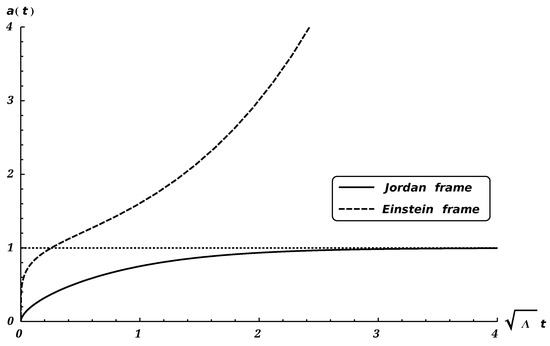
Figure 1. Scale factors $a_{\lambda <0}^{(-)}$ and ${\overline{a}}_{\lambda <0}^{(+)}$ as functions of time $\sqrt{\Lambda t}$.

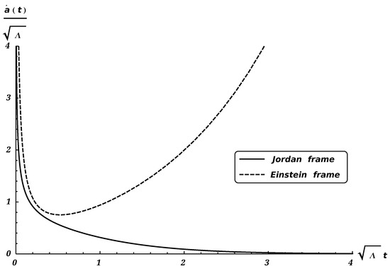
Figure 2. Scale factor velocities ${\dot{a}}_{\lambda <0}^{(-)}/\sqrt{\Lambda }$ and ${\dot{\overline{a}}}_{\lambda <0}^{(+)}/\sqrt{\Lambda }$ as functions of time $\sqrt{\Lambda t}$.

Figure 3 shows the behavior of the deceleration parameter $q\left(t\right)$ as function of time $\sqrt{\Lambda t}$ in both frames. We conclude from this figure that in the Jordan frame the deceleration parameter has a positive sign, which may be interpreted as a matter dominated era. In the Einstein frame the behavior of the deceleration parameter is different from that of the Jordan frame. At the begin the deceleration parameter has positive sign and evolves to a negative sign. Here it may be interpreted to an exit of a matter dominated period to a dark energy era.

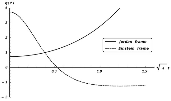
Figure 3. Deceleration parameters $q_{\lambda <0}^{(+)}$ and ${\overline{q}}_{\lambda <0}^{(-)}$ as functions of time $\sqrt{\Lambda t}$.

It is clear that in this work we introduced only one constituent which is the scalar field. In order to have a better insight of the cosmological behavior one should add a matter constituent. This will be the subject of a next investigation.

8. Conclusions

In this work we analyzed a model with a scalar field minimally coupled to gravity. We started with the action in the Einstein frame and obtained the action in the Jordan frame through the use of the Weyl transformations. The field equations in the Jordan frame were obtained from the Palatini variation method. By restricting to a spatially flat Friedman–Robertson–Walker metric the point-like Lagrangian and the equations of Friedmann acceleration and Klein–Gordon were obtained. The Noether symmetry method was used to determine the self-interaction potential of the scalar field. From the solution of the field equations the scale factor, the Hubble and deceleration parameters were obtained in the Jordan frame and the corresponding ones in the Einstein frame were determined by the use of Weyl transformations. The cosmological solutions were obtained in case where the coupling constant of the scalar field $\omega =1/2$ which corresponds to a the case of a minimally coupled scalar field in the Einstein frame. It was show that in the Jordan frame the scalar factor grows with time but tends to a constant value at large times, i.e., evolving into a stationary universe. Furthermore, its deceleration parameter has a positive sign, which may be interpreted as a matter dominated era. In the Einstein frame the scale factor grows with time and the deceleration parameter evolves from a positive sign to a negative one, which may be interpreted as a transition from a matter dominated period to a dark energy era.

References

- Will, C.M. The Confrontation between General Relativity and Experiment. Living Rev. Rel. 2014, 17, 4. [Google Scholar] [CrossRef] [PubMed]
- Yunes, N.; Siemens, X. Gravitational-Wave Tests of General Relativity with Ground-Based Detectors and Pulsar Timing-Arrays. Living Rev. Rel. 2013, 16, 9. [Google Scholar] [CrossRef] [PubMed]
- Capozziello, S.; De Laurentis, M. Extended Theories of Gravity. Phys. Rept. 2011, 509, 167–321. [Google Scholar] [CrossRef]
- Capozziello, S.; Lambiase, G.; Sakellariadou, M.; Stabile, A. Constraining models of extended gravity using Gravity Probe B and LARES experiments. Phys. Rev. 2015, D91, 044012. [Google Scholar] [CrossRef]
- Brans, C.; Dicke, R.H. Mach’s principle and a relativistic theory of gravitation. Phys. Rev. 1961, 124, 925–935. [Google Scholar] [CrossRef]
- Sen, D.K.; Dunn, K.A. A Scalar-Tensor Theory of Gravitation in a Modified Riemannian Manifold. J. Math. Phys. 1971, 12, 578–586. [Google Scholar] [CrossRef]
- Dunn, K.A. A scalar-tensor theory of gravitation. J. Math. Phys. 1974, 15, 2229–2231. [Google Scholar] [CrossRef]
- Faraoni, V.; Côté, J.; Giusti, A. Do solar system experiments constrain scalar–tensor gravity? Eur. Phys. J. C 2020, 80, 132. [Google Scholar] [CrossRef]
- Burton, H.; Mann, R.B. Palatini variational principle for an extended Einstein-Hilbert action. Phys. Rev. 1998, D57, 4754–4759. [Google Scholar] [CrossRef]
- Kozak, A.; Borowiec, A. Palatini frames in scalar–tensor theories of gravity. Eur. Phys. J. C 2019, 79, 335. [Google Scholar] [CrossRef]
- Almeida, T.S.; Pucheu, M.L.; Romero, C.; Formiga, J.B. From Brans-Dicke gravity to a geometrical scalar-tensor theory. Phys. Rev. D 2014, 89, 064047. [Google Scholar] [CrossRef]
- Pucheu, M.L.; Alves Junior, F.A.P.; Barreto, A.; Romero, C. Cosmological models in Weyl geometrical scalar-tensor theory. Phys. Rev. D 2016, 94, 064010. [Google Scholar] [CrossRef]
- Capozziello, S.; de Ritis, R.; Marino, A.A. Conformal equivalence and Noether symmetries in cosmology. Class. Quant. Grav. 1998, 14, 3259. [Google Scholar] [CrossRef]
- Paliathanasis, A. Using Noether symmetries to specify f(R) gravity. J. Phys. Conf. Ser. 2013, 453, 012009. [Google Scholar] [CrossRef]
- Terzis, P.A.; Dimakis, N.; Christodoulakis, T. Noether analysis of Scalar-Tensor Cosmology. Phys. Rev. D 2014, 90, 123543. [Google Scholar] [CrossRef]
- Camci, U. F(R,G) Cosmology through Noether Symmetry Approach. Symmetry 2018, 10, 719. [Google Scholar] [CrossRef]
- de Souza, R.C.; Kremer, G.M. Constraining non-minimally coupled tachyon fields by Noether symmetry. Class. Quant. Grav. 2009, 26, 135008. [Google Scholar] [CrossRef]
- de Souza, R.C.; Kremer, G.M. Dark Sector from Interacting Canonical and Non-Canonical Scalar Fields. Class. Quant. Grav. 2010, 27, 175006. [Google Scholar] [CrossRef][Green Version]
- de Souza, R.C.; Kremer, G.M. Cosmic expansion from boson and fermion fields. Class. Quant. Grav. 2011, 28, 125006. [Google Scholar] [CrossRef]
- de Souza, R.C.; Andre, R.; Kremer, G.M. Analysis of the nonminimally coupled scalar field in the Palatini formalism by the Noether symmetry approach. Phys. Rev. D 2013, 87, 083510. [Google Scholar] [CrossRef]
- Romero, C.; Fonseca-Neto, J.B.; Pucheu, M.L. General Relativity and Weyl Geometry. Class. Quant. Grav. 2012, 29, 155015. [Google Scholar] [CrossRef]
- Scholz, E. MOND-like acceleration in integrable Weyl geometric gravity. Found. Phys. 2016, 46, 176. [Google Scholar] [CrossRef]
© 2020 by the authors. Licensee MDPI, Basel, Switzerland. This article is an open access article distributed under the terms and conditions of the Creative Commons Attribution (CC BY) license (http://creativecommons.org/licenses/by/4.0/).