A Sparse Quasi-Newton Method Based on Automatic Differentiation for Solving Unconstrained Optimization Problems

Abstract

In our paper, we introduce a sparse and symmetric matrix completion quasi-Newton model using automatic differentiation, for solving unconstrained optimization problems where the sparse structure of the Hessian is available. The proposed method is a kind of matrix completion quasi-Newton method and has some nice properties. Moreover, the presented method keeps the sparsity of the Hessian exactly and satisfies the quasi-Newton equation approximately. Under the usual assumptions, local and superlinear convergence are established. We tested the performance of the method, showing that the new method is effective and superior to matrix completion quasi-Newton updating with the Broyden–Fletcher–Goldfarb–Shanno (BFGS) method and the limited-memory BFGS method.

1. Introduction

We concentrated on the unconstrained optimization problem

$$minf\left(x\right),x\in R^n,$$

(1)

where $f:R^n\to R$ is a twice continuously differentiable function; and $\nabla f\left(x\right)$ and ${\nabla }^{2}f\left(x\right)$ denote the gradient and Hessian of f at x, respectively. The first order necessary condition of (1) is

$$\nabla f\left(x\right)=0,$$

which can be written as the symmetric nonlinear equations

$$F\left(x\right)=0,$$

(2)

where $F:R^n\to R^n$ is a continuously differentiable mapping and the symmetry implies that the Jacobian $F^{\prime }\left(x\right)$ satisfies $F^{\prime }\left(x\right)=F^{\prime }{\left(x\right)}^T$. That symmetric nonlinear system has close relationships with many practical problems, such as the gradient mapping of unconstrained optimization problems, the Karush–Kuhn–Tuckrt (KKT) system of equality constrained optimization problem, the discretized two-point boundary value problem, and the saddle point problem (2) [1,2,3,4,5].

For small or medium-scale problems, classical quasi-Newton methods enjoy superlinear convergence without the calculation of the Hessian [6,7]. Let $x_k$ be the current iterative point and $B_k$ be the symmetric approximation of the Hessian; then the iteration $\left\{x_k\right\}$ generated by quasi-Newton methods is

$$x_{k+1}=x_k+{\alpha }_k{d}_k\nabla f\left(x_k\right),$$

where ${\alpha }_k>0$ is a step length obtained by some line search or other strategies. The search direction $d_k$ can be gotten by solving the equations

$$B_k{d}_k+\nabla f\left(x_k\right)=0,$$

where the quasi-Newton matrix $B_k$ is an approximation of ${\nabla }^{2}f\left(x_k\right)$ and satisfies the secant condition:

$$B_{k+1}{s}_k=y_k,$$

where $s_k=x_{k+1}-x_k$, $y_k=\nabla f\left(x_{k+1}\right)-\nabla f\left(x_k\right)$. The matrix $B_k$ can be updated by different update formulae. The Davidon–Fletcher–Powell (DFP) update,

$$\begin{array}{ccc}\hfill B_{k+1}& =& \left(I-\frac{y_k{s}_k^T}{y_k^T{s}_k}\right)B_k\left(I-\frac{y_k{s}_k^T}{y_k^T{s}_k}\right)+\frac{y_k{y}_k^T}{y_k^T{s}_k}\hfill \\ & =& B_k+\frac{(y_k-B_k{s}_k)s_k^T+s_k{(y_k-B_k{s}_k)}^T}{y_k^T{s}_k}\hfill \\ & & -\frac{{(y_k-B_k{s}_k)}^T{s}_k}{{\left(y_k^T{s}_k\right)}^2}{y}_k{y}_k^T\hfill \\ & =& \left(I-\frac{y_k{s}_k^T}{y_k^T{s}_k}\right)B_k\left(I-\frac{y_k{s}_k^T}{y_k^T{s}_k}\right)+\frac{y_k{y}_k^T}{y_k^T{s}_k},\hfill \end{array}$$

was first proposed by Davidon [8] and developed by Fletcher and Powell [9]. The Broyden–Fletcher–Goldfard–Shanno (BFGS) update,

$$B_{k+1}=B_k-\frac{B_k{s}_k{s}_k^T{B}_k}{s_k^T{B}_k{s}_k}+\frac{y_k{y}_k^T}{y_k^T{s}_k},$$

was proposed independently by Broyden [10], Fletcher [11], Goldfarb [12], and Shanno [13]. One can find more on the topic in references [14,15,16,17].

If we assume that $H_k=B_k^{-1}$, then using Sherman–Morrison formula, we have the Broyden’s family update:

$$H_{k+1}=H_k-\frac{H_k{y}_k{y}_k^T{H}_k}{y_k^T{H}_k{y}_k}+\frac{s_k{s}_k^T}{s_k^T{y}_k}+{\varphi }_k{v}_k{v}_k^T,$$

where ${\varphi }_k\in [0,1]$ is

$${\varphi }_k=\sqrt{y_k^T{H}_k{y}_k}\left(\frac{s_k}{s_k^T{y}_k}-\frac{H_k{y}_k}{y_k^T{H}_k{y}_k}\right),$$

When ${\varphi }_k\equiv 1$, we have a BFGS update. When ${\varphi }_k\equiv 0$, we have a DFP update.

However, a quasi-Newton method is not desirable when applied to solve large-scale problems, because we need to store the full matrx $B_k$. To overcome such drawback, the so-called sparse quasi-Newton methods [14] have received much attention. Early in 1970, Schubert [18] has proposed a sparse Broyden’s rank one method. Then Powell and Toint [19], Toint [20] studied the sparse quasi-Newton method.

Existing sparse quasi-Newton methods usually use a sparse symmetric matrix as an approximation of the Hessian so that both matrices take the same form or have similar structures. If the limited memory technique [21,22] is adopted, which only stores several pairs $(s_k,y_k)$ to construct a matrix $H_k$ by updating the initial matrix $H_0$m times, the method can be widely used in practical optimization problems. On the other hand, there are many large-scale problems in scientific fields take the partially separable form

$$f\left(x\right)=\sum _{i=1}^m{f}_i\left(x\right),$$

where function $f_i$, $i=1,\dots ,m$ is related to a few variables. For the partially separable unconstrained optimization problems, the partitioned BFGS method [23,24] was proposed and has better performance in practice. The partitioned BFGS method updates each matrix $B_k^i$ of each element function $f_i\left(x\right)$ separately via BFGS updating and sums these matrices to construct the next quasi-Newton matrix $B_{k+1}$. Since the size of x in $f_i\left(x\right)$ is smaller than that of n, the matrix $B_{k+1}^i$ will be a small matrix, and then the matrix $B_{k+1}$ will be sparse. The quasi-Newton direction is the solution of the linear equations:

$$\left(\sum _{i=1}^m{B}_k^i\right)d_k=-\nabla f\left(x_k\right).$$

However, the partitioned BFGS method cannot always preserve the positive definiteness of the matrix $B_k$, only if that each element function $f_i\left(x\right)$ is convex, so the partitioned BFGS method is implemented with the trust region strategy [25]. Recently, for the partially separable nonlinear equations, Cao and Li [26] have introduced two kinds of partitioned quasi-Newton methods and given their global and superlinear convergence.

Another efficient sparse quasi-Newton method is designed to exploit the sparsity structures of the Hessian. We assume that for all $x\in R^n$,

$${\left({\nabla }^{2}f\left(x\right)\right)}_{i,j}=0,(i,j)\in F,$$

where $F\subseteq \{1,\dots ,n\}\times \{1,\dots ,n\}$. References  [27,28] have proposed sparse quasi-Newton methods, where $H_{k+1}$ satisfies the secant equation

$$H_{k+1}{y}_k=s_k$$

and sparse condition

$${\left(H_{k+1}\right)}_{ij}=0,(i,j)\in F$$

simultaneously, where $H_{k+1}$ is an approximate inverse Hessian. Recently, Yamashita [29] proposed another type of matrix completion quasi-Newton (MCQN) update for solving problem (1) with a sparse Hessian and proved the local and superlinear convergence for MCQN updates with the DFP method. Reference [30] established the convergence of MCQN updates with all of Broyden’s convex family. However, global convergence analysis [31] was presented for two-dimensional functions with uniformly positive definite Hessians.

Another kind of quasi-Newton method for solving large scale unconstrained optimization problems is the diagonal quasi-Newton method, where the Hessian of an objective function is approximated by a diagonal matrix with positive elements. The first version was developed by Nazareth [32], where the quasi-Newton matrix satisfies the least change and weak secant condition [33]:

$$\begin{array}{ccc}\hfill min& & \Vert H_{k+1}-H_k\Vert \hfill \\ \hfill \mathrm{s.t.}& & y_k^T{H}_{k+1}{y}_k=y_k^T{s}_k,\hfill \end{array}$$

(3)

where ${\Vert ·\Vert }_F$ is the standard Frobenius norm. Recently, Andrei N. [34] developed a diagonal quasi-Newton method, where the diagonal elements satisfy the least change weak secant condition (3) and minimize the trace of the update. Besides, lots of other techniques, such as forward and central finite differences, the variational principle with a weighted norm, and the generalized Frobenius norm, can be used to derive different kinds of diagonal quasi-Newton method [35,36,37]. Under usual assumptions, the diagonal quasi-Newton method is linearly convergent. The authors of [38] adopted a similar technique to derivation with the DFP method and got a low memory diagonal quasi-Newton method. Using the Armijo line search, they established the global convergence and gave the sufficient conditions for the method to be superlinearly convergent.

The main contribution of our paper is to propose a sparse quasi-Newton algorithm based on automatic differentiation for solving (1). Firstly, similarly to the derivation of BFGS update, we can perform a symmetric rank-two quasi-Newton update:

$$B_{k+1}=B_k-\frac{B_k{\sigma }_k{\sigma }_k^T{B}_k}{{\sigma }_k^T{B}_k{\sigma }_k}+\frac{{\nabla }^{2}f\left(x_{k+1}\right){\sigma }_k{\sigma }_k^T{\nabla }^{2}f\left(x_{k+1}\right)}{{\sigma }_k^T{\nabla }^{2}f\left(x_{k+1}\right){\sigma }_k},$$

(4)

where ${\sigma }_k\in R^n$ and $B_{k+1}$ satisfying the adjoint tangent condition [39]

$${\sigma }_k^T{B}_{k+1}={\sigma }_k^T{\nabla }^{2}f\left(x_{k+1}\right).$$

For an $n\times n$ matrix, we denote $A⪰0$, as A is positive definite. Then, when $B_k⪰0$, $B_{k+1}⪰0$ if and only if ${\sigma }_k^T{\nabla }^{2}f\left(x_{k+1}\right){\sigma }_k>0$, which means that the proposed update (4) keeps the positive definiteness, as in BFGS updating. Moreover, when $B_0$ is positive definite, the matrices $\left\{B_k\right\}$ updated by the proposed update (4) are positive definite for solving (1) with uniformly positive definite Hessians. In our work, we pay attention to ${\sigma }_k=s_k$; then the proposed rank-two quasi-Newton update (4) method satisfies

$$B_{k+1}{s}_k={\nabla }^{2}f\left(x_{k+1}\right)s_k,$$

which means that $B_{k+1}$ equals ${\nabla }^{2}f\left(x_{k+1}\right)$ in the direction $s_k$ exactly. Several lemmas have been given to present the properties of the proposed rank-two quasi-Newton update formula. Secondly, combined with the idea of MCQN method [29], we propose a sparse and symmetric quasi-Newton algorithm for solving (1). Under appropriate conditions, local and superlinear convergence are established. Finally, our numerical results illustrate that the proposed algorithm has satisfying performance.

The paper is organized as follows. In Section 2, we introduce a symmetric rank-two quasi-Newton update based on automatic differentiation and prove several nice properties. In Section 3, by using the idea of matrix completion, we present a sparse quasi-Newton algorithm and show some nice properties. In Section 4, we prove the local and superlinear convergence of the algorithm proposed in Section 3. Numerical results are listed in Section 5, which verify that the proposed algorithm is very encouraging. Finally, we give the conclusion.

2. A New Symmetric Rank-Two Quasi–Newton Update

Similarly to the derivation of BFGS update, we will derive a new symmetric rank-two quasi-Newton update and show several lemmas. Let

$$B_{k+1}=B_k+{∆}_k,$$

where ${∆}_k$ is a rank-two matrix and $B_{k+1}$ satisfies the condition

$${\sigma }_k^T{B}_{k+1}={\sigma }_k^T{\nabla }^{2}f\left(x_{k+1}\right),$$

(5)

where ${\sigma }_k\in R^n$ and ${\sigma }_k\ne 0$. Similarly to the derivation of BFGS, we have the following symmetric rank-two update:

$$B_{k+1}=B_k-\frac{B_k{\sigma }_k{\sigma }_k^T{B}_k}{{\sigma }_k^T{B}_k{\sigma }_k}+\frac{{\nabla }^{2}f\left(x_{k+1}\right){\sigma }_k{\sigma }_k^T{\nabla }^{2}f\left(x_{k+1}\right)}{{\sigma }_k^T{\nabla }^{2}f\left(x_{k+1}\right){\sigma }_k}.$$

(6)

If we denote $H_k=B_k^{-1}$ and $H_{k+1}=B_{k+1}^{-1}$, then (6) can be expressed as

$$\begin{array}{ccc}\hfill H_{k+1}& =& H_k-\frac{H_k{\nabla }^{2}f\left(x_{k+1}\right){\sigma }_k{\sigma }_k^T+{\sigma }_k{\sigma }_k^T{\nabla }^{2}f\left(x_{k+1}\right)H_k}{{\sigma }_k^T{\nabla }^{2}f\left(x_{k+1}\right){\sigma }_k}\hfill \\ & & +\left(1+\frac{{\sigma }_k^T{\nabla }^{2}f\left(x_{k+1}\right)H_k{\nabla }^{2}f\left(x_{k+1}\right){\sigma }_k}{{\sigma }_k^T{\nabla }^{2}f\left(x_{k+1}\right){\sigma }_k}\right)·\frac{{\sigma }_k{\sigma }_k^T}{{\sigma }_k^T{\nabla }^{2}f\left(x_{k+1}\right){\sigma }_k}.\hfill \end{array}$$

(7)

It can be seen that the update (6) involves the Hessian ${\nabla }^{2}f\left(x\right)$, but we do not need to compute them in practice. For given vectors x, s, and $\sigma$, we can get ${\nabla }^{2}f\left(x\right)s$ and ${\sigma }^T{\nabla }^{2}f\left(x\right)$ exactly by the forward and reverse mode of automatic differentiation.

Next, several lemmas are presented.

Lemma 1.

We suppose that $B_k⪰0$ and $B_{k+1}$ is updated by (6); then $B_{k+1}⪰0$ if and only if ${\sigma }_k^T{\nabla }^{2}f\left(x_{k+1}\right){\sigma }_k>0$.

Proof. 

According to the condition (5), one has

$${\sigma }_k^T{\nabla }^{2}f\left(x_{k+1}\right){\sigma }_k={\sigma }_k^T{B}_{k+1}{\sigma }_k.$$

If $B_{k+1}$ is positive definite, one has ${\sigma }_k^T{\nabla }^{2}f\left(x_{k+1}\right){\sigma }_k>0$.

Let ${\sigma }_k^T{\nabla }^{2}f\left(x_{k+1}\right){\sigma }_k>0$ and $B_k⪰0$. Then for $\forall d_k\in R^n$, $d_k\ne 0$, it can be derived from (6) that

$$d_k^T{B}_{k+1}{d}_k=d_k^T{B}_k{d}_k-\frac{{\left(d_k^T{B}_k{\sigma }_k\right)}^2}{{\sigma }_k^T{B}_k{\sigma }_k}+\frac{{\left(d_k^T{\nabla }^{2}f\left(x_{k+1}\right){\sigma }_k\right)}^2}{{\sigma }_k^T{\nabla }^{2}f\left(x_{k+1}\right){\sigma }_k}.$$

According to that $B_k⪰0$, there is a symmetric matrix $B_k^{1/2}⪰0$, such that $B_k=B_k^{1/2}{B}_k^{1/2}$. Then we have from Cauchy–Schwarz inequality that

$$\begin{array}{ccc}\hfill {\left(d_k^T{B}_k{\sigma }_k\right)}^2& =& {\left({\left(B_k^{1/2}{d}_k\right)}^T\left(B_k^{1/2}{\sigma }_k\right)\right)}^2\hfill \\ & \le & \Vert B_k^{1/2}{d}_k{\Vert }^2·{\Vert B_k^{1/2}{\sigma }_k\Vert }^2\hfill \\ & =& \left(d_k^T{B}_k{d}_k\right)\left({\sigma }_k^T{B}_k{\sigma }_k\right),\hfill \end{array}$$

(8)

where the equality holds if and only if $d_k={\lambda }_k{\sigma }_k$, ${\lambda }_k\ne 0$.

If the inequality (8) holds strictly, one has

$$d_k^T{B}_{k+1}{d}_k>d_k^T{B}_k{d}_k-d_k^T{B}_k{d}_k+\frac{{\left(d_k^T{\nabla }^{2}f\left(x_{k+1}\right){\sigma }_k\right)}^2}{{\sigma }_k^T{\nabla }^{2}f\left(x_{k+1}{\sigma }_k\right)}\ge 0.$$

If the equality (8) holds; i.e., there exists a ${\lambda }_k\ne 0$ such that $d_k={\lambda }_k{\sigma }_k$, then it can be deduced from (8) that

$$d_k^T{B}_{k+1}{d}_k\ge \frac{{\left(d_k^T{\nabla }^{2}f\left(x_{k+1}\right){\sigma }_k\right)}^2}{{\sigma }_k^T{\nabla }^{2}f\left(x_{k+1}{\sigma }_k\right)}={\lambda }_k^2{\sigma }_k^T{\nabla }^{2}f\left(x_{k+1}\right){\sigma }_k>0.$$

In conclusion, $d_k^T{B}_{k+1}{d}_k>0$ for $\forall d_k\in R^n$ and $d_k\ne 0$.    □

Lemma 2.

If we rewrite update Formula (7) as $H_{k+1}=H_k+E$, where $H_k$ is symmetric and satisfies ${\sigma }_k^T={\sigma }_k^T{\nabla }^{2}f\left(x_{k+1}\right)H_k$, then E is the solution of the following minimization problem:

$$\begin{array}{ccc}\hfill \underset{E}{min}& & {\Vert E\Vert }_W\hfill \\ \hfill s.t.& & E^T=E,\hfill \\ & & {\sigma }_k^T{\nabla }^{2}f\left(x_{k+1}\right)E={\eta }^T,\hfill \end{array}$$

where $\eta ={\sigma }_k^T-{\sigma }_k^T{\nabla }^{2}f\left(x_{k+1}\right)H_k$ and W satisfies ${\sigma }_k^{T}W={\sigma }_k^T{\nabla }^{2}f\left(x_{k+1}\right)$.

Proof. 

A suitable Lagrangian function of the convex programming problem is

$$\phi =\frac{1}{4}\mathrm{trace}\left(W{E}^{T}WE\right)+\mathrm{trace}\left({\mathrm{\Lambda }}^T(E^T-E)\right)-{\lambda }^{T}W(E{\nabla }^{2}f\left(x_{k+1}\right){\sigma }_k-\eta ),$$

where $\mathrm{\Lambda }$ and $\lambda$ are Lagrange multipliers. Moreover,

$$\begin{array}{ccc}\hfill \frac{\partial \phi }{\partial E_{ij}}& =& \frac{1}{4}(\mathrm{trace}\left(W{e}_j{e}_i^{T}WE\right)+\mathrm{trace}\left(W{E}^{T}W{e}_i{e}_j^T\right))\hfill \\ & & +\mathrm{trace}\left(\mathrm{\Lambda }(e_j{e}_i^T-e_i{e}_j^T)\right)-{\lambda }^{T}W{e}_i{e}_j^T{F}^{\prime }\left(x_{k+1}\right){\sigma }_k=0,\hfill \end{array}$$

or according to the symmetry and cyclic permutations, one has

$$\frac{1}{2}{\left[WEW\right]}_{ij}+{\mathrm{\Lambda }}_{ij}-{\mathrm{\Lambda }}_{ji}={\left[W\lambda {\sigma }_k^T{\nabla }^{2}f\left(x_{k+1}\right)\right]}_{ij}.$$

Taking the transpose and accumulating eliminates $\mathrm{\Lambda }$ to yield

$$WEW=W\lambda {\sigma }_k^T{\nabla }^{2}f\left(x_{k+1}\right)+{\nabla }^{2}f\left(x_{k+1}\right){\sigma }_k{\lambda }^{T}W,$$

and by ${\sigma }_k^{T}W={\sigma }_k^T{\nabla }^{2}f\left(x_{k+1}\right)$ and the nonsingularity of W we have that

$$E=\lambda {\sigma }_k^T+{\sigma }_k{\lambda }^T.$$

(9)

Substituting (9) into ${\sigma }_k^T{\nabla }^{2}f\left(x_{k+1}\right)E={\eta }^T$ and rewriting gives

$$\lambda =\frac{\eta -{\sigma }_k{\lambda }^T{\nabla }^{2}f\left(x_{k+1}\right){\sigma }_k}{{\sigma }_k^T{\nabla }^{2}f\left(x_{k+1}\right){\sigma }_k}.$$

Postmultiplying by ${\sigma }_k^T{\nabla }^{2}f\left(x_{k+1}\right)$ gives

$${\lambda }^T{\nabla }^{2}f\left(x_{k+1}\right){\sigma }_k=\frac{1}{2}\frac{{\sigma }_k^T{\nabla }^{2}f\left(x_{k+1}\right)\eta }{{\sigma }_k^T{\nabla }^{2}f\left(x_{k+1}\right){\sigma }_k},$$

so we have

$$\lambda =\frac{\eta -\frac{1}{2}\frac{{\sigma }_k^T{\sigma }_k{\nabla }^{2}f\left(x_{k+1}\right)\eta }{{\sigma }_k^T{\nabla }^{2}f\left(x_{k+1}\right){\sigma }_k}}{{\sigma }_k^T{\nabla }^{2}f\left(x_{k+1}\right){\sigma }_k}=\frac{H_k{\nabla }^{2}f\left(x_{k+1}\right){\sigma }_k-\frac{1}{2}\frac{{\sigma }_k^T{\sigma }_k{\nabla }^{2}f\left(x_{k+1}\right)H{\nabla }^{2}f\left(x_{k+1}\right){\sigma }_k}{{\sigma }_k^T{\nabla }^{2}f\left(x_{k+1}\right){\sigma }_k}}{{\sigma }_k^T{\nabla }^{2}f\left(x_{k+1}\right){\sigma }_k}.$$

Substituting this into (9) gives the result (7).    □

Lemma 3.

If $H_k=B_k^{-1}>0$ and ${\sigma }_k^T{\nabla }^{2}f\left(x_{k+1}\right){\sigma }_k>0$. Then $B_{k+1}$ given by (6) solves the variational problem

$$\begin{array}{ccc}\hfill \underset{B>0}{min}& & \psi \left(H_k^{1/2}B{H}_k^{1/2}\right)\hfill \\ \hfill s.t.& & B^T=B,\hfill \\ & & {\sigma }_k^{T}B={\sigma }_k^T{\nabla }^{2}f\left(x_{k+1}\right).\hfill \end{array}$$

Proof. 

According to the definition of $\psi$, where $\psi :R^{n\times n}\to R$ [40] is given by

$$\psi \left(A\right)=\mathrm{tr}\left(A\right)-lndet\left(A\right),$$

(10)

so we have

$$\psi \left(H_k^{1/2}B{H}_k^{1/2}\right)=\mathrm{trace}\left(H_{k}B\right)-\ln \left(\det H_k\det B\right)=\psi \left(H_{k}B\right)=\psi \left(B{H}_k\right).$$

(11)

We have the Lagrangian function

$$\begin{array}{ccc}\hfill L(B,\mathrm{\Lambda },\lambda )& =& \frac{1}{2}\psi \left(H_k^{1/2}B{H}_k^{1/2}\right)+\mathrm{trace}({\mathrm{\Lambda }}^T(B^T-B)+({\sigma }_k^{T}B-{\sigma }_k^T{\nabla }^{2}f\left(x_{k+1}\right)){\lambda }_k\hfill \\ & =& \frac{1}{2}(\psi \left(H_{k}B\right)-\ln \left(\det H_k\right)-\ln \left(\det B\right))\hfill \\ & & +\mathrm{trace}\left({\mathrm{\Lambda }}^T(B^T-B)\right)+({\sigma }_k^{T}B-{\sigma }_k^T{\nabla }^{2}f\left(x_{k+1}\right)){\lambda }_k,\hfill \end{array}$$

where $\mathrm{\Lambda }$ and $\lambda$ are the Lagrange multipliers. Moreover, one has

$$\begin{array}{ccc}\hfill \frac{\partial L}{\partial B_{ij}}& =& \frac{1}{2}\mathrm{trace}\left(H_k{e}_i{e}_j^T-{\left(B^{-1}\right)}_{ji}\right)+\mathrm{trace}\left({\mathrm{\Lambda }}^T(e_k{e}_i^T-e_i{e}_j^T)\right)+{\sigma }_k^T{e}_i{e}_j^T\lambda \hfill \\ & =& \frac{1}{2}{\left(H_k\right)}_{ji}-{\left(B^{-1}\right)}_{ji})+{\mathrm{\Lambda }}_{ji}-{\mathrm{\Lambda }}_{ij}+{\left({\sigma }_k^T\lambda \right)}_{ij}=0.\hfill \end{array}$$

(12)

Transposing and adding in (12) that

$$\begin{gathered} H_k-B^{-1}+{\sigma }_k^T\lambda +{\lambda }^T{\sigma }_k=0, \\ {B}^{-1}=H_k+{\sigma }_k^T\lambda +{\lambda }^T{\sigma }_k. \end{gathered}$$

(13)

Combined with the tangent condition, we have that

$${\sigma }_k^T={\sigma }_k^T{\nabla }^{2}f\left(x_{k+1}\right)H_k+{\sigma }_k^T{\nabla }^{2}f\left(x_{k+1}\right)\lambda {\sigma }_k^T+{\sigma }_k^T{\nabla }^{2}f\left(x_{k+1}\right){\sigma }_k{\lambda }^T,$$

and hence

$${\sigma }_k^T{\nabla }^{2}f\left(x_{k+1}\right){\sigma }_k=\frac{1}{2}\left(1-\frac{{\sigma }_k^T{\nabla }^{2}f\left(x_{k+1}\right)H_k{\nabla }^{2}f\left(x_{k+1}\right){\sigma }_k}{{\sigma }_k^T{\nabla }^{2}f\left(x_{k+1}\right){\sigma }_k}\right),$$

and so

$$\lambda =\frac{{\sigma }_k-H_k{\nabla }^{2}f\left(x_{k+1}\right)-\frac{1}{2}\left(1-\frac{{\sigma }_k^T{\nabla }^{2}f\left(x_{k+1}\right)H_k{\nabla }^{2}f\left(x_{k+1}\right){\sigma }_k}{{\sigma }_k^T{\nabla }^{2}f\left(x_{k+1}\right){\sigma }_k}\right)}{{\sigma }_k^T{\nabla }^{2}f\left(x_{k+1}\right){\sigma }_k}.$$

Combined with (6), one has the Formula (7).

According to the Sherman–Morrison formula, (7) is equivalent to (6). Since the function $\psi \left(H_k^{1/2}B{H}_k^{1/2}\right)$ is strictly convex on $B⪰0$, the update formula (6) is the unique solution of the variational problem.    □

In this paper, we set ${\sigma }_k=s_k$, so one has

$$B_{k+1}{s}_k={\nabla }^{2}f\left(x_{k+1}\right)s_k,$$

which means that $B_{k+1}$ is an exact approximation to ${\nabla }^{2}f\left(x_{k+1}\right)$ in direction $s_k$. Then we have the symmetric rank-two update formula

$$B_{k+1}=B_k-\frac{B_k{s}_k{s}_k^T{B}_k}{s_k^T{B}_k{s}_k}+\frac{{\nabla }^{2}f\left(x_{k+1}\right)s_k{s}_k^T{\nabla }^{2}f\left(x_{k+1}\right)}{s_k^T{\nabla }^{2}f\left(x_{k+1}\right)s_k}.$$

(14)

It can be seen that $B_{k+1}$ can preserve the symmetry when $B_k$ is symmetric. If we denote $w_k={\nabla }^{2}f\left(x_{k+1}\right)s_k$, then we can obtain a similar Broyden convex family update formula:

$$H_{k+1}=H_k-\frac{H_k{w}_k{w}_k^T{H}_k}{w_k^T{H}_k{w}_k}+\frac{s_k{s}_k^T}{s_k^T{w}_k}+{\varphi }_k{v}_k{v}_k^T,$$

(15)

where the parameter ${\varphi }_k\in [0,1]$ is defined as

$$v_k=\sqrt{w_k^T{H}_k{w}_k}\left(\frac{s_k}{s_k^T{w}_k}-\frac{H_k{w}_k}{w_k^T{H}_k{w}_k}\right).$$

(16)

The choice ${\varphi }_k\equiv 1$ corresponds to the BFGS update

$$\begin{array}{ccc}\hfill H_{k+1}& =& H_k+\left(1+\frac{w_k^T{H}_k{w}_k}{s_k^T{w}_k}\right)\frac{s_k^T{s}_k}{s_k^T{w}_k}-\frac{s_k^T{w}_k{H}_k+H_k{w}_k{s}_k^T}{s_k^T{w}_k}\hfill \\ & =& H_k+\frac{(s_k-H_k{w}_k)s_k^T+s_k{(s_k-H_k{w}_k)}^T}{s_k^T{w}_k}.\hfill \end{array}$$

(17)

3. Algorithm and Related Properties

For the update formula (15), we adopt the idea of matrix completion. The next quasi-Newton matrix $H_{k+1}$ is the solution of the following minimization problem:

$$\begin{array}{ccc}\hfill min& & \psi \left(H_k^{-1/2}H{H}_k^{-1/2}\right)\hfill \\ \hfill \mathrm{s.t.}& & H_{ij}=H_{i,j}^{AD},(i,j)\in F,\hfill \\ & & {\left(H^{-1}\right)}_{i,j}=0,(i,j)\notin F,\hfill \\ & & H^T=H,H⪰0.\hfill \end{array}$$

(18)

When $G(V,\overline{F})$ is chordal, the minimization problem (18) can be solved by solving the problem

$$\begin{array}{ccc}\hfill max& & det\left(H\right)\hfill \\ \hfill \mathrm{s.t.}& & H_{i,j}=H_{i,j}^{AD},(i,j)\in F,\hfill \\ & & H^T=H,H⪰0.\hfill \end{array}$$

(19)

Then $H_{k+1}$ can be expressed as the sparse clique-factorization formula [29]. Then Algorithm 1 is stated as follows.

Algorithm 1 (Sparse Quasi-Newton Algorithm based on Automatic Differentiation)

Step 0. Compute $\overline{F}$ according to F such that $G(V,\overline{F})$ is a chordal graph, where    $V=\{1,2,\cdots ,n\}$. Choose $x_0\in R^n$, $ϵ>0$ and a matrix $H_0\in R^{n\times n},$ $H_0⪰0$ with ${\left(H_0^{-1}\right)}_{ij}=0$, $\forall (i,j)\notin F$. Let $k:=0$. Step 1 If $\Vert \nabla f\left(x_k\right)\Vert ⩽ϵ$, stop. Step 2$x_{k+1}=x_k-H_k\nabla f\left(x_k\right)$. Step 3 Update $H_k$ to get $H_{ij}^{AD},{\varphi }_k\in [0,1]$, $(i,j)\in F$ by update Formula (15). Step 4 Get $H_{k+1}$ by the minimization problem (18). When $G(V,\overline{F})$ is a chordal graph, the problem (18) can be solved by solving the problem (19). Step 5 Let $k:=k+1$, go to Step 1.

When the $H_k$ in step 3 is updated by Broyden’s class method, the method corresponds to the method in [29]. In the present paper, we focus on the MCQN update with $H^{AD}=H_{k+1}$, where $H_{k+1}$ is given by (15).

In what follows, we give some notation for the convenience of analysis. For a nonsingular matrix P satisfying

$${\left(P^{-1}\right)}_{ij}=0,\forall (i,j)\in F,$$

(20)

we let

$${\overline{s}}_k=P^{-1/2}{s}_k,{\overline{w}}_k=P^{1/2}{w}_k,{\overline{H}}_k=P^{-1/2}{H}_k{P}^{-1/2},{\overline{H}}^{AD}=P^{-1/2}{H}^{AD}{P}^{-1/2},$$

where $H^{AD}=H_{k+1}$ is given by (15). Then we can get from (15) that

$${\overline{H}}^{AD}={\overline{H}}_k-\frac{{\overline{H}}_k{\overline{w}}_k{\overline{w}}_k^T{\overline{H}}_k}{{\overline{w}}_k^T{\overline{H}}_k{\overline{w}}_k}+\frac{{\overline{s}}_k{\overline{s}}_k^T}{{\overline{s}}_k^T{\overline{w}}_k}+{\varphi }_k{\overline{v}}_k{\overline{v}}_k^T,$$

(21)

where

$${\overline{v}}_k=\sqrt{{\overline{w}}_k^T{\overline{H}}_k{\overline{w}}_k}\left(\frac{{\overline{s}}_k}{{\overline{s}}_k^T{\overline{w}}_k}-\frac{{\overline{H}}_k{\overline{w}}_k}{{\overline{w}}_k^T{\overline{H}}_k{\overline{w}}_k}\right).$$

(22)

Similarly to that in [30], we can assume that

$${\tau }_k=\frac{{\overline{w}}_k^T{\overline{H}}_k{\overline{w}}_k^T}{\Vert {\overline{w}}_k\Vert ·\Vert {\overline{H}}_k{\overline{w}}_k\Vert },q_k=\frac{{\overline{w}}_k^T{\overline{H}}_k{\overline{w}}_k}{\Vert {\overline{w}}_k{\Vert }^2},{\eta }_k=\frac{{\overline{s}}_k^T{\overline{H}}_k{\overline{w}}_k}{{\overline{s}}_k^T{\overline{w}}_k},m_k=\frac{{\overline{s}}_k^T{\overline{w}}_k}{{\overline{w}}_k^T{\overline{w}}_k},$$

$$M_k=\frac{\Vert {\overline{s}}_k{\Vert }^2}{{\overline{s}}_k^T{\overline{w}}_k},{\beta }_k=\frac{{\overline{s}}_k^T{\overline{H}}_k^{-1}{\overline{s}}_k^T}{{\overline{s}}_k^T{\overline{w}}_k},{\gamma }_k=\frac{{\overline{w}}_k^T{\overline{H}}_k{\overline{w}}_k}{{\overline{s}}_k^T{\overline{w}}_k}.$$

According to [41] and (21), we have

$$\mathrm{tr}\left({\overline{H}}^{AD}\right)=\mathrm{tr}\left({\overline{H}}_k\right)-(1-{\varphi }_k)\frac{q_k}{{\tau }_k^2}-2{\varphi }_k{\eta }_k+\left(1+{\varphi }_k\frac{q_k}{m_k}\right)M_k$$

(23)

and

$$\det \left({\overline{H}}^{AD}\right)=\det \left({\overline{H}}_k\right)\left(1+{\varphi }_k({\beta }_k{\gamma }_k-1)\right)/{\gamma }_k.$$

(24)

Next, we establish a relation between ${\overline{H}}_{k+1}$ and ${\overline{H}}^{AD}$, which is very important in the establishment of the local and superlinear convergence of Algorithm 1.

Proposition 1.

For the Algorithm 1, we have the following relation:

$$tr\left({\overline{H}}_{k+1}\right)=tr\left({\overline{H}}^{AD}\right),det\left({\overline{H}}_{k+1}\right)⩾det\left({\overline{H}}^{AD}\right).$$

(25)

Proof. 

We can obtain from (18) that

$${\left(H_{k+1}\right)}_{i,j}={\left(H^{AD}\right)}_{i,j},\forall (i,j)\in F.$$

Combined with (20), one has that for any $(i,j)\in F$, there at least exists one of the ${(H_{k+1}-H^{AD})}_{ij}$ and $P_{i,j}^{-1}$ equals to zero. Then we can get that

$$\begin{array}{ccc}\hfill \mathrm{tr}({\overline{H}}_{k+1}-{\overline{H}}^{AD})& =& \mathrm{tr}\left(P^{-1}(H_{k+1}-H^{AD})\right)\hfill \\ & =& \sum _{i=1}^n\sum _{j=1}^n{\left(P^{-1}\right)}_{i,j}{(H_{k+1}-H^{AD})}_{i,j}=0.\hfill \end{array}$$

(26)

Moreover, since $H^{AD}$ satisfies (19), we must have

$$det\left(H_{k+1}\right)⩾det\left(H^{AD}\right).$$

Consequently, one has

$$\begin{array}{c}\hfill det\left({\overline{H}}_{k+1}\right)={\overline{H}}^{AD}.\end{array}$$

(27)

□

Remark 1.

According to the definition of ψ (10) and the relation between ${\overline{H}}_{k+1}$ and ${\overline{H}}^{AD}$(25), one has that

$$\psi \left({\overline{H}}_{k+1}\right)⩽\psi \left({\overline{H}}^{AD}\right).$$

(28)

When we substitute (23) and (24) into (28), the $\psi \left({\overline{H}}_{k+1}\right)$ and $\psi \left({\overline{H}}_k\right)$ has the relation

$$\begin{array}{ccc}\hfill \psi \left({\overline{H}}_{k+1}\right)& ⩽& \psi \left({\overline{H}}_k\right)-(1-{\varphi }_k)\frac{q_k}{{\tau }_k^2}-2{\varphi }_k{\eta }_k+\left(1+{\varphi }_k\frac{q_k}{m_k}\right)M_k\hfill \\ & & -ln\left(1+{\varphi }_k({\beta }_k{\gamma }_k-1)\right)+ln{\gamma }_k.\hfill \end{array}$$

(29)

4. The Local and Superlinear Convergence

Based on the discussion in Section 3, we prove the local and superlinear convergence of Algorithm 1. First, we list the assumptions.

Assumption A1.

Assume that $x^{\ast }$ is a solution of (1) and

$$]\mathrm{\Omega }=\{x\in R^n|\Vert x-x^{\ast }\Vert ⩽b\},$$

where $b>0$.

(1) 

The function $f\in R^n\to R$ is twice continuously differentiable on Ω.

(2) 

There exist two constants, $m>0$ and $M>0$, satisfying

$${m\Vert u\Vert }^2⩽u^T{\left({\nabla }^{2}f\left(x\right)\right)}^{-1}u⩽M{\Vert u\Vert }^2,\forall u\in R^n,x\in \mathrm{\Omega }.$$

(30)

According to Assumption 1, we have constants $\overline{L}>0$ and $L>0$ such that

$$\Vert \nabla f\left(x\right)-\nabla f\left(y\right)\Vert ⩽\overline{L}\Vert x-y\Vert ,\forall x,y\in \mathrm{\Omega },$$

(31)

$$\Vert {\nabla }^{2}f\left(x\right)-{\nabla }^{2}f\left(y\right)\Vert ⩽L\Vert x-y\Vert ,\forall x,y\in \mathrm{\Omega }.$$

(32)

We define

$${ϵ}_k=max\{\Vert x_k-x^{\ast }\Vert ,\Vert x_{k+1}-x^{\ast }\Vert \},$$

(33)

and get from (32) that

$$\begin{array}{ccc}\hfill \Vert w_k-{\nabla }^{2}f\left(x^{\ast }\right)s_k\Vert & =& \Vert {\nabla }^{2}f\left(x_{k+1}\right)s_k-{\nabla }^{2}f\left(x^{\ast }\right)s_k\Vert \hfill \\ & ⩽& \Vert {\nabla }^{2}f\left(x_{k+1}\right)-{\nabla }^{2}f\left(x^{\ast }\right)\Vert ·\Vert s_k\Vert \hfill \\ & ⩽& L\Vert x_{k+1}-x^{\ast }\Vert ·\Vert s_k\Vert \hfill \\ & =& L{ϵ}_k\Vert s_k\Vert .\hfill \end{array}$$

(34)

If we take $P=H^{\ast }$, then one has from (34) that

$$\begin{array}{ccc}\hfill \Vert {\overline{w}}_k-{\overline{s}}_k\Vert & =& \Vert P^{1/2}{w}_k-P^{-1/2}{s}_k\Vert \hfill \\ & =& \Vert {H^{\ast }}^{1/2}\Vert ·\Vert w_k-{\nabla }^{2}f\left(x^{\ast }\right)s_k\Vert ⩽L\Vert H^{\ast }{\Vert }^{1/2}{ϵ}_k\Vert s_k\Vert ,\hfill \end{array}$$

(35)

Furthermore, it is easy to deduce that

$$M_k-1,{\mu }_k=\frac{2-M_k-m_k}{m_k},{\widehat{\mu }}_k=\frac{{({\overline{w}}_k-{\overline{s}}_k)}^T{\overline{H}}_k{\overline{w}}_k}{\mathrm{tr}\left({\overline{H}}_k\right){\overline{s}}_k^T{\overline{w}}_k},ln{m}_k⩽\frac{1}{2}{c}_1{ϵ}_k,$$

(36)

where $c_1>0$, $c_2\in (0,b)$, and ${ϵ}_k<c_2$. We define

$$\begin{array}{ccc}\hfill {\rho }_k& =& q_k-1-ln{q}_k,\hfill \\ \hfill {\zeta }_k& =& (1-{\varphi }_k)q_k({\tau }_k^{-2}-1),\hfill \\ \hfill {\xi }_k& =& ln(1+{\varphi }_k({\beta }_k{\gamma }_k-1)),\hfill \end{array}$$

(37)

and rewrite (29) as

$$\begin{array}{ccc}\hfill \psi \left({\overline{H}}_{k+1}\right)& ⩽& \psi \left({\overline{H}}_k\right)-{\rho }_k-{\zeta }_k-{\xi }_k+(M_k-1)\hfill \\ & & +{\varphi }_k{q}_k{\mu }_k+{\varphi }_k\mathrm{tr}\left({\overline{H}}_k\right){\widehat{\mu }}_k+ln{m}_k.\hfill \end{array}$$

(38)

As ${\gamma }_k=q_k/m_k$ and $0⩽q_k⩽\mathrm{tr}\left({\overline{H}}_k\right)$, we can obtain from the above inequality and (36) that

$$\psi \left({\overline{H}}_{k+1}\right)⩽\psi \left({\overline{H}}_k\right)-{\rho }_k-{\zeta }_k-{\xi }_k+c_1\left(1+\mathrm{tr}\left({\overline{H}}_k\right)\right){ϵ}_k.$$

(39)

Considering

$$\lambda -ln\lambda ⩾max\left(\left(1-\frac{1}{e}\right)\lambda ,1\right),\forall \lambda >0,$$

(40)

one has

$$\psi \left(A\right)⩾max\left(\left(1-\frac{1}{e}\right)\mathrm{tr}\left(A\right),n\right),$$

where $A^T=A$ and $A>0$. Moreover, it follows from (40) that

$$\psi \left({\overline{H}}_{k+1}\right)⩽(1+c_3{ϵ}_k)\psi \left({\overline{H}}_k\right)-{\rho }_k-{\zeta }_k-{\xi }_k,$$

(41)

where $c_3=c_1\left(\frac{1}{n}+\frac{e}{e-1}\right)$. Since ${\tau }_k^2⩽1$ and ${\beta }_k{\gamma }_k⩾1$, it is obvious that ${\rho }_k,{\zeta }_k,{\xi }_k>0$, and

$$\psi \left({\overline{H}}_{k+1}\right)⩽(1+c_3{ϵ}_k)\psi \left({\overline{H}}_k\right).$$

(42)

The theorem given bellow shows that Algorithm 1 converges locally and linearly, where the relation (42) plays an essential role.

Theorem 1.

Let Assumption 1 hold and sequence $\left\{x_k\right\}$ be generated by Algorithm 1 with ${\alpha }_k\equiv 1$, where $H_k$ is updated by (15). Then for any $\rho \in (0,1)$, there is a constant τ $\Vert x_0-x^{\ast }\Vert ⩽\tau$, $\Vert H_0-H^{\ast }\Vert ⩽\tau$, such that

$$\Vert x_{k+1}-x^{\ast }\Vert ⩽\rho \Vert x_k-x^{\ast }\Vert .$$

(43)

Proof. 

According to the Lemma 4 [29], there are constants $\overline{\tau }\in (0,b)$ and $\delta >0$ such that when $\Vert x_0-x^{\ast }\Vert ⩽\overline{\tau }$, one has

$$\psi \left({\overline{H}}_0\right)-n⩽\delta /2,$$

(44)

and

$$\Vert H-H^{\ast }\Vert ⩽\rho /\left(2\overline{L}\right),$$

(45)

where $H⪰0$ and $\overline{H}={H^{\ast }}^{-1/2}H\overline{H}={H^{\ast }}^{-1/2}$. Define

$$\tau =min\left\{\overline{\tau },c_2,\frac{\rho }{\overline{L}},\frac{\rho }{LM},\frac{1-\rho }{c_3}ln\left(\frac{2(n+\delta )}{2n+\delta }\right)\right\}.$$

(46)

We will prove the inequalities (43) and

$$\Vert H_k-H^{\ast }\Vert ⩽\frac{\rho }{2\overline{L}}$$

(47)

hold for any $k⩾0$ by induction. By the Lipstchitz continuity of ${\nabla }^{2}f\left(x\right)$, we have for $\forall x\in \mathrm{\Omega }$,

$$\begin{array}{ccc}\hfill \Vert x-x^{\ast }-H^{\ast }\nabla f\left(x\right)\Vert & ⩽& \parallel H^{\ast }\Vert ·{\int }_0^1\Vert {\nabla }^{2}f(x+t(x-x^{\ast }))-{\nabla }^{2}f\left(x^{\ast }\right)\Vert ·\Vert x-x^{\ast }\Vert dt\hfill \\ & ⩽& \frac{1}{2}LM{\Vert x-x^{\ast }\Vert }^2.\hfill \end{array}$$

(48)

Then, when $k=0$, it is easy to deduce (43) by (44) and (45). Moreover, when we take ${\alpha }_k\equiv 1$ and substitute $x_0$ into (48), we can obtain

$$\begin{array}{ccc}\hfill \Vert x_1-x^{\ast }\Vert & =& \Vert x_0-H_0\nabla f\left(x_0\right)-x^{\ast }\Vert \hfill \\ & ⩽& \Vert x_0-x^{\ast }-H^{\ast }\nabla f\left(x_0\right)\Vert +\Vert (H_0-H^{\ast })(\nabla f\left(x_0\right))-\nabla f\left(x^{\ast }\right))\Vert \hfill \\ & ⩽& \frac{1}{2}LM\Vert x_0-x^{\ast }{\Vert }^2+\Vert H_0-H^{\ast }\Vert ·\Vert \nabla f\left(x_0\right))-\nabla f\left(x^{\ast }\right)\Vert \hfill \\ & ⩽& \left(\frac{1}{2}LM\Vert x_0-x^{\ast }\Vert +\frac{\rho }{2}\right)\Vert x_0-x^{\ast }\Vert \hfill \\ & ⩽& \left(\frac{1}{2}LM\tau +\frac{\rho }{2}\right)\Vert x_0-x^{\ast }\Vert \hfill \\ & ⩽& \rho \Vert x_0-x^{\ast }\Vert .\hfill \end{array}$$

(49)

So we have that (43) and (47) hold for $k=1$. Assume that (43) and (47) hold for $k=0,1,\dots ,l$; then one has

$${ϵ}_k=\Vert x_k-x^{\ast }\Vert ,{ϵ}_k⩽{\rho }^k{ϵ}_0⩽{\rho }^k\tau ,k=0,1,\dots ,l,$$

and

$$\begin{array}{ccc}\hfill \Vert x_{l+1}-x^{\ast }\Vert & =& \Vert x_l-H_l\nabla f\left(x_l\right)-x^{\ast }\Vert \hfill \\ & ⩽& \Vert x_l-x^{\ast }-H^{\ast }\nabla f\left(x_l\right)\Vert +\Vert (H_l-H^{\ast })(\nabla f\left(x_l\right))-\nabla f\left(x^{\ast }\right))\Vert \hfill \\ & ⩽& \frac{1}{2}LM\Vert x_l-x^{\ast }{\Vert }^2+\Vert H_l-H^{\ast }\Vert ·\Vert \nabla f\left(x_l\right))-\nabla f\left(x^{\ast }\right)\Vert \hfill \\ & ⩽& \left(\frac{1}{2}LM\Vert x_l-x^{\ast }\Vert +\frac{\rho }{2}\right)\Vert x_l-x^{\ast }\Vert \hfill \\ & ⩽& \left(\frac{1}{2}LM{\rho }^l\tau +\frac{\rho }{2}\right)\Vert x_l-x^{\ast }\Vert \hfill \\ & ⩽& \rho \Vert x_l-x^{\ast }\Vert .\hfill \end{array}$$

(50)

Then by the definition of $\tau$ (46), one has

$$c_3\sum _{k=0}^l{ϵ}_k⩽c_3\tau \sum _{k=0}^l{\rho }^k=c_3\tau \frac{1-{\rho }^{l+1}}{1-\rho }⩽\frac{c_3\tau }{1-\rho }⩽ln\frac{2(n+\delta )}{2n+\delta }.$$

(51)

Combine (42) and (44). It can seen that

$$\begin{array}{ccc}\hfill \psi \left({\overline{H}}_{l+1}\right)-n& ⩽& (\psi \left({\overline{H}}_0\right)-n)+\left(\prod _{k=0}^l(1+c_3{ϵ}_k)-1\right)\psi \left({\overline{H}}_0\right)\hfill \\ & ⩽& \frac{\delta }{2}+\left(n+\frac{\delta }{2}\right)\left(\prod _{k=0}^l{e}^{c_3{ϵ}_k}-1\right)\hfill \\ & ⩽& \frac{\delta }{2}+\left(n+\frac{\delta }{2}\right)\left(e^{c_3{\sum }_{k=0}^l{ϵ}_k}-1\right)\hfill \\ & ⩽& \frac{\delta }{2}+\left(n+\frac{\delta }{2}\right)\left(\frac{2(n+\delta )}{2n+\delta }-1\right)=\delta .\hfill \end{array}$$

(52)

Thus, we can get that (47) holds for all $k=l+1$. This completes the proof. □

Based on the above discussion and the relation (42), we can show the superlinear convergence of the Algorithm 1.

Theorem 2.

Let Assumption A1 hold and sequence $\left\{x_k\right\}$ be generated by Algorithm 1 with ${\alpha }_k\equiv 1$, where $H_k$ is updated by (15). Then there is a constant $\tau >0$ such that when $\Vert x_0-x^{\ast }\Vert ⩽\tau$, $\Vert H_0-H^{\ast }\Vert ⩽\tau$, one has

$$\underset{k\to \infty }{lim}\frac{\Vert (H_k-H^{\ast })w_k\Vert }{\Vert w_k\Vert }=0.$$

(53)

Then the sequence $\left\{x_k\right\}$ is superlinearly convergent.

Proof. 

Let $\tau$ be defined as in (1), and for all k one has

$$\psi \left({\overline{H}}_k\right)-n⩽\delta .$$

(54)

It follows from (41) that

$${\rho }_k+{\zeta }_k+{\xi }_k⩽\left(\psi \left({\overline{H}}_{k+1}\right)-\psi \left({\overline{H}}_k\right)\right)+c_3{ϵ}_k\psi \left({\overline{H}}_k\right).$$

Summing the above inequality and combining (51) and (54), we can deduce

$$\sum _{k⩾1}({\rho }_k+{\zeta }_k+{\xi }_k)⩽c_3\sum _{k⩾1}{ϵ}_k\psi \left({\overline{H}}_k\right)⩽c_3(n+\delta )ln\frac{2(n+\delta )}{2n+\delta }<\infty ,$$

(55)

which means that the nonnegative constants ${\rho }_k$, ${\zeta }_k$ and ${\xi }_k$ all tend to zero when $k\to +\infty$. Furthermore, according to the definition of (37), we have that

$$\left(1\right)q_k\to 1;\left(2\right)\mathrm{if}{\varphi }_k⩽\frac{1}{2},\tau \to 1;\left(3\right)\mathrm{if}{\varphi }_k>\frac{1}{2},{\beta }_k{\gamma }_k\to 1.$$

First, we have

$$\begin{array}{ccc}\hfill \frac{\Vert {H^{\ast }}^{-1/2}(H_k-H^{\ast })w_k{\Vert }^2}{\Vert {H^{\ast }}^{1/2}{w}_k{\Vert }^2}& =& \frac{\Vert {\overline{H}}_k{\overline{w}}_k{\Vert }^2-2{\overline{w}}_k^T{\overline{H}}_k{\overline{w}}_k+{\Vert {\overline{w}}_k\Vert }^2}{\Vert {\overline{H}}_k{\Vert }^2}\hfill \\ & =& \frac{q_k}{{\tau }_k^2}-2q_k+1.\hfill \end{array}$$

(56)

For the case $\{k_i:{\varphi }_{k_i}⩽\frac{1}{2}\}$, one has $q_k\to 1$, and ${\tau }_{k_i}\to 1$; and then (53) is true.

Moreover, it is easy to deduce that

$$\begin{array}{ccc}\hfill \frac{\Vert {\overline{H}}_k{\overline{w}}_k-{\overline{s}}_k{\Vert }^2}{\Vert {\overline{w}}_k{\Vert }^2}& ⩽& \frac{\Vert {\overline{H}}_k^{1/2}{\Vert }^2·{\Vert {\overline{H}}_k^{1/2}{\overline{w}}_k-{\left({\overline{H}}_k\right)}^{-1/2}{\overline{s}}_k\Vert }^2}{\Vert {\overline{w}}_k{\Vert }^2}\hfill \\ & =& \frac{\Vert {\overline{H}}_k^{1/2}{\Vert }^2({\overline{w}}_k^T{\overline{H}}_k{\overline{w}}_k-2{\overline{s}}_k^T{\overline{w}}_k+{\overline{s}}_k^T{\left({\overline{H}}_k\right)}^{-1}{\overline{s}}_k)}{\Vert {\overline{w}}_k{\Vert }^2}\hfill \\ & =& \Vert {\overline{H}}_k^{1/2}{\Vert }^2\left(q_k-2m_k+\frac{{\beta }_k{\gamma }_k}{q_k}\right).\hfill \end{array}$$

(57)

We also have

$$|\frac{\Vert {\overline{H}}_k{\overline{w}}_k-{\overline{w}}_k\Vert }{\Vert {\overline{w}}_k\Vert }-\frac{\Vert {\overline{H}}_k{\overline{w}}_k-{\overline{s}}_k\Vert }{\Vert {\overline{w}}_k\Vert }|⩽\frac{\Vert {\overline{w}}_k-{\overline{s}}_k\Vert }{\Vert {\overline{w}}_k\Vert }\to 0.$$

(58)

For the case $\{k_i:{\varphi }_{k_i}>\frac{1}{2}\}$, one has $q_k\to 1$, ${\beta }_k{\gamma }_k\to 1$, $m_k\to 1$; then (53) is true by (56)–(58). Thus, the relation (53) holds for all k.

Next, we will show that (53) indicates that the sufficient condition [6]

$$\underset{k\to \infty }{lim}\frac{\Vert (B_k-{\nabla }^{2}f\left(x^{\ast }\right))s_k\Vert }{\Vert s_k\Vert }=0$$

(59)

holds. According to (47), one has that there is a constant ${\lambda }_{min}>0$ such that ${\left({\lambda }_k\right)}_i⩾{\lambda }_{min}$, where ${\left({\lambda }_k\right)}_i$ denotes the eigenvalues of $H_k$, $i=1,2,\cdots ,n$. When we let $w_k={\nabla }^{2}f\left(x_{k+1}\right)s_k$, one has

$$\begin{array}{ccc}& & \Vert (H_k-H^{\ast })w_k\Vert \hfill \\ & =& \Vert (H_k-H^{\ast }){\nabla }^{2}f\left(x^{\ast }\right)s_k+(H_k-H^{\ast })({\nabla }^{2}f\left(x_{k+1}\right)-{\nabla }^{2}f\left(x^{\ast }\right))s_k\Vert \hfill \\ & ⩾& \Vert H_k({\nabla }^{2}f\left(x^{\ast }\right)-B_k)s_k\Vert -\Vert (H_k-H^{\ast })({\nabla }^{2}f\left(x_{k+1}\right)-{\nabla }^{2}f\left(x^{\ast }\right))s_k\Vert \hfill \\ & ⩾& {\lambda }_{min}\Vert ({\nabla }^{2}f\left(x^{\ast }\right)-B_k)s_k\Vert -\Vert (H_k-H^{\ast })({\nabla }^{2}f\left(x_{k+1}\right)-{\nabla }^{2}f\left(x^{\ast }\right))s_k\Vert ,\hfill \end{array}$$

and

$$\begin{array}{ccc}& & \frac{\Vert (H_k-H^{\ast })w_k\Vert }{\Vert w_k\Vert }\hfill \\ & =& \frac{{\lambda }_{min}\Vert ({\nabla }^{2}f\left(x^{\ast }\right)-B_k)s_k\Vert }{\Vert {\nabla }^{2}f\left(x_{k+1}\right)s_k\Vert }-\frac{\Vert (H_k-H^{\ast })({\nabla }^{2}f\left(x_{k+1}\right)-{\nabla }^{2}f\left(x^{\ast }\right))s_k\Vert }{\Vert {\nabla }^{2}f\left(x_{k+1}\right)s_k\Vert }\hfill \\ & ⩾& \frac{{\lambda }_{min}\Vert ({\nabla }^{2}f\left(x^{\ast }\right)-B_k)s_k\Vert }{\frac{1}{{\lambda }_{min}}\Vert s_k\Vert }-\frac{\Vert (H_k-H^{\ast })({\nabla }^{2}f\left(x_{k+1}\right)-{\nabla }^{2}f\left(x^{\ast }\right))s_k\Vert }{\frac{1}{{\lambda }_{min}}\Vert s_k\Vert }\hfill \\ & =& {\lambda }_{min}^2\Vert ({\nabla }^{2}f\left(x^{\ast }\right)-B_k)\Vert -{\lambda }_{min}\Vert (H_k-H^{\ast })({\nabla }^{2}f\left(x_{k+1}\right)-{\nabla }^{2}f\left(x^{\ast }\right))\Vert .\hfill \end{array}$$

When $k\to \infty$, since $x_k\to x^{\ast }$, then one has from (53) that

$$\underset{k\to \infty }{lim}\frac{\Vert (B_k-{\nabla }^{2}f\left(x^{\ast }\right))s_k\Vert }{\Vert s_k\Vert }=0,$$

which is the well-known Dennis–Moré condition. Thus, we get the superlinear convergence. □

5. Numerical Experiments

The performance in [29] shows that the MCQN update with the BFGS method has better numerical performance than the MCQN update with DFP method. Hence, we compare the numerical performance of Algorithm 1 with the MCQN update with BFGS method and the limited-memory BFGS method.

The 24 test problems with initial points are given in Table 1, which are from [29,42,43,44]. It can be seen that all the test problems have special Hessian structures such as band matrices, so the chordal extension of the sparsity could be obtained easily. Then $H_{k+1}$ in Algorithm 1 can be written as the sparse clique-factorization formula.

Table 1. The test problems.

Pro	the Test Functions	Init
1	TRIDIA [29]	$x_0={(1,1,\cdots ,1)}^T$
2	the chained Rosenbrock problem [29]	$x_0={(-1.2,-1,\dots ,-1.2,-1)}^T$
3	the boundary value problem [29]	$x_0={(\frac{1}{n+1},\frac{2}{n+1}\cdots ,\frac{n}{n+1})}^T$
4	Broyden tridiagonal function [42]	$x_0={(-1,-1,\cdots ,-1)}^T$
5	DQRTIC [43]	$x_0={(2,2,\cdots ,2)}^T$
6	EDENSCH [43]	$x_0={(0,0,\cdots ,0)}^T$
7	ENGVAL1 [43]	$x_0={(2,2,\cdots ,2)}^T$
8	COSINE [43]	$x_0={(1,1,\cdots ,1)}^T$
9	ERRINROS-modified [43]	$x_0={(-1,-1,\cdots ,-1)}^T$
10	FREUROTH [43]	$x_0={(0.5,-2,0,\cdots ,0)}^T$
11	MOREBV- different start point [43]	$x_0={(0.5,0.5,\cdots ,0.5)}^T$
12	TOINTGSS [43]	$x_0={(3,3,\cdots ,3)}^T$
13	SCHMVETT [43]	$x_0={(3,3,\cdots ,3)}^T$
14	Extended Freudenstein and Roth function [44]	$x_0={(0.5,-2,\cdots ,0.5,-2)}^T$
15	Raydan 1 function [44]	$x_0={(1,1,\cdots ,1)}^T$
16	Generalized Tridiagonal function [44]	$x_0={(2,2,\cdots ,2)}^T$
17	Extended Himmelblau function [44]	$x_0={(1,1,\cdots ,1)}^T$
18	Generalized PSCI function [44]	$x_0={(3,0.1,\cdots ,3,0.1)}^T$
19	Extended Tridiagonal 2 function [44]	$x_0={(1,1,\cdots ,1)}^T$
20	Raydan 2 function [44]	$x_0={(1,1,\cdots ,1)}^T$
21	Extended Freudenstein and Roth function [44]	$x_0={(1,1,\cdots ,1)}^T$
22	DQDRTIC function [44]	$x_0={(3,3,\cdots ,3)}^T$
23	Generalized Quartic function [44]	$x_0={(1,1,\cdots ,1)}^T$
24	HIMMELBG function [44]	$x_0={(1.5,1.5,\cdots ,1.5)}^T$

All the methods were coded in MATLAB R2016a on a Core (TM) i5 PC. The automatic differentiation was computed by ADMAT 2.0, which is available on the cayuga research GitHUB page. In Table 1, Table 2, Table 3 and Table 4 and Figure 1 and Figure 2, we report the numerical performances of the three methods. For the convenience of statement, we use the following notation in our numerical results.

Table 2. Numbers of iterations for problems 1–12.

Dim	10	20	50	100	200	500	1000	2000	5000	10,000
(1) Algorithm 1	30	38	51	78	96	146	217	301	424	527
(1) MCQN-BFGS	29	38	51	72	95	146	192	298	424	528
(1) L-BFGS	26	39	96	158	360	864	1042	1759	3153	3152
(2) Algorithm 1	49	90	166	308	595	1345	2699	5437	3218	2725
(2) MCQN-BFGS	60	95	200	384	683	1668	3249	6486	4562	3207
(2) L-BFGS	59	113	260	504	999	2481	4947	9887	24,732	49,391
(3) Algorithm 1	16	26	42	58	59	51	49	60	102	399
(3) MCQN-BFGS	15	26	42	50	59	71	54	69	101	402
(3) L-BFGS	39	114	279	700	1503	1659	2695	3370	8867	27,471
(4) Algorithm 1	31	25	34	49	43	44	43	49	52	53
(4) MCQN-BFGS	30	29	43	45	49	58	61	62	63	56
(4) L-BFGS	21	27	40	54	41	38	38	56	52	50
(5) Algorithm 1	30	48	60	92	109	99	92	89	81	81
(5) MCQN-BFGS	35	49	67	94	111	108	112	98	84	84
(5) L-BFGS	28	27	34	31	33	39	41	43	54	81
(6) Algorithm 1	23	26	38	44	54	55	47	51	61	51
(6) MCQN-BFGS	17	27	36	53	60	55	54	51	50	54
(6) L-BFGS	17	19	19	22	21	23	24	26	24	25
(7) Algorithm 1	16	21	21	19	17	17	16	15	16	15
(7) MCQN-BFGS	20	22	23	22	15	15	15	17	17	16
(7) L-BFGS	20	22	26	21	22	21	25	27	28	30
(8) Algorithm 1	22	23	24	21	23	27	27	28	29	30
(8) MCQN-BFGS	23	25	26	26	26	27	28	28	29	30
(8) L-BFGS	9	9	9	9	10	10	10	10	10	10
(9) Algorithm 1	74	122	134	149	137	180	148	153	172	170
(9) MCQN-BFGS	106	125	145	171	199	181	168	171	174	179
(9) L-BFGS	163	245	216	196	189	190	163	169	171	192
(10) Algorithm 1	45	45	48	39	45	43	45	145	161	145
(10) MCQN-BFGS	47	48	49	43	47	48	41	244	204	279
(10) L-BFGS	24	25	24	24	24	22	22	22	20	22
(11) Algorithm 1	24	45	97	121	82	67	35	34	21	11
(11) MCQN-BFGS	24	45	98	121	82	67	35	34	21	11
(11) L-BFGS	33	103	136	127	85	49	32	21	10	9
(12) Algorithm 1	13	11	11	12	9	5	6	2	3	2
(12) MCQN-BFGS	15	11	13	12	12	7	6	2	3	2
(12) L-BFGS	6	8	9	10	13	11	10	10	9	10

Table 3. Numbers of iterations for problems 13–24.

Dim	10	20	50	100	200	500	1000	2000	5000	10,000
(13) Algorithm 1	19	20	21	22	18	17	15	14	13	12
(13) MCQN-BFGS	19	20	21	22	18	17	15	14	13	12
(13) L-BFGS	16	18	17	18	18	17	18	18	17	18
(14) Algorithm 1	36	52	95	111	169	262	612	567	1062	1114
(14) MCQN-BFGS	37	54	86	120	190	300	594	679	1062	1126
(14) L-BFGS	10	10	10	10	10	10	10	10	10	11
(15) Algorithm 1	11	13	23	30	39	45	60	97	196	295
(15) MCQN-BFGS	11	12	21	28	37	45	64	95	196	295
(15) L-BFGS	13	21	32	50	79	122	207	338	402	770
(16) Algorithm 1	29	31	47	69	110	149	165	174	170	163
(16) MCQN-BFGS	29	35	51	70	100	146	164	173	171	164
(16) L-BFGS	25	65	80	162	160	156	151	150	144	140
(17) Algorithm 1	16	15	14	11	13	12	12	12	10	9
(17) MCQN-BFGS	14	11	18	12	13	12	12	12	10	9
(17) L-BFGS	8	8	8	8	8	8	8	8	8	8
(18) Algorithm 1	49	21	23	21	19	14	22	21	13	11
(18) MCQN-BFGS	43	28	22	29	20	15	20	25	23	26
(18) L-BFGS	36	34	37	36	39	36	40	34	41	37
(19) Algorithm 1	13	12	11	13	12	12	12	10	7	5
(19) MCQN-BFGS	13	12	11	13	12	12	12	10	7	5
(19) L-BFGS	12	14	15	16	16	17	16	15	16	17
(20) Algorithm 1	5	5	4	4	4	4	4	3	3	3
(20) MCQN-BFGS	5	5	4	4	4	4	4	3	3	3
(20) L-BFGS	7	7	7	7	7	7	7	7	7	7
(21) Algorithm 1	14	11	11	21	18	18	35	28	26	43
(21) MCQN-BFGS	13	10	11	22	18	18	35	28	26	43
(21) L-BFGS	10	13	15	19	22	30	36	51	56	64
(22) Algorithm 1	36	36	26	28	26	27	27	30	28	29
(22) MCQN-BFGS	36	36	26	28	26	27	27	30	28	29
(22) L-BFGS	13	13	16	16	17	16	16	15	19	19
(23) Algorithm 1	13	17	12	21	12	14	8	11	10	9
(23) MCQN-BFGS	16	18	22	25	15	13	12	13	12	10
(23) L-BFGS	14	14	16	15	17	24	27	27	27	31
(24) Algorithm 1	11	13	18	24	31	37	28	21	13	7
(24) MCQN-BFGS	12	15	19	25	32	37	28	21	13	7
(24) L-BFGS	10	10	10	10	10	10	10	10	10	10

Table 4. Results of Dim = 1000 with different initial points.

Pro	Algorithm 1					MCQN-BFGS
Init	${\mathit{x}}_{\mathbf{0}}$	$\mathbf{2}{\mathit{x}}_{\mathbf{0}}$	$\mathbf{4}{\mathit{x}}_{\mathbf{0}}$	$\mathbf{7}{\mathit{x}}_{\mathbf{0}}$	$\mathbf{10}{\mathit{x}}_{\mathbf{0}}$	${\mathit{x}}_{\mathbf{0}}$	$\mathbf{2}{\mathit{x}}_{\mathbf{0}}$	$\mathbf{4}{\mathit{x}}_{\mathbf{0}}$	$\mathbf{7}{\mathit{x}}_{\mathbf{0}}$	$\mathbf{10}{\mathit{x}}_{\mathbf{0}}$
(1)	217	189	192	194	196	192	210	213	220	213
(2)	2699	2684	2641	1192	2694	3249	4850	5056	2157	4961
(3)	49	47	55	68	65	54	213	210	228	294
(4)	43	47	36	81	80	60	213	210	228	294
(5)	92	83	86	91	89	112	106	85	94	94
(6)	47	47	47	47	47	54	54	54	54	54
(7)	16	30	53	19	21	15	19	27	21	22
(8)	27	31	16	35	54	28	31	16	33	56
(9)	148	159	154	184	157	168	151	147	191	154
(10)	45	45	164	170	175	41	263	203	192	194
(11)	35	70	96	112	127	35	70	96	112	127
(12)	6	6	2	2	2	6	6	2	2	2
(13)	15	16	17	14	14	15	16	17	14	14
(14)	612	312	504	511	318	594	523	503	481	563
(15)	60	57	208	452	1024	64	58	203	532	941
(16)	165	180	173	153	129	164	183	191	197	215
(17)	12	11	10	7	21	12	11	8	7	30
(18)	22	23	25	60	41	20	23	30	65	75
(19)	12	12	14	16	24	12	12	14	22	20
(20)	4	6	5	6	4	4	6	5	6	4
(21)	35	30	35	112	719	35	30	35	112	719
(22)	27	28	28	29	29	27	28	28	29	29
(23)	8	22	23	14	35	12	13	24	19	70
(24)	28	20	21	21	21	28	20	21	21	21

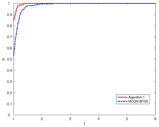
Figure 1. Performance profiles based on the numbers of iterations.

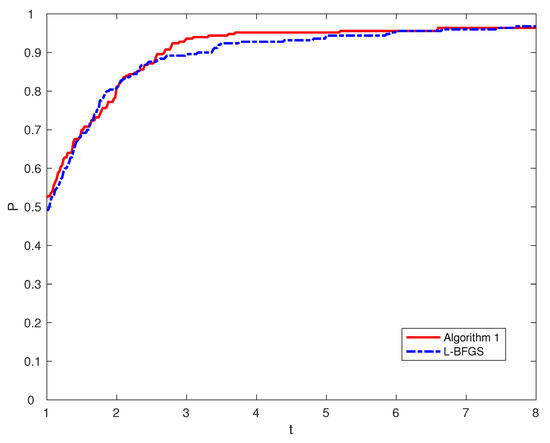
Figure 2. Performance profiles based on the numbers of iterations.

• Pro: the problems;
• Dim: the dimensions of the test problem;
• Init: the initial points;
• Method: the algorithm used to solve the problem;
• MCQN-BFGS: MCQN update with the BFGS method;
• L-BFGS: limited-memory with the BFGS method.

We adopted the termination criterion as follows:

$$\frac{\Vert \nabla f\left(x\right)\Vert }{n}⩽{10}^{-5}\mathrm{or}\mathrm{ite}⩾5000.$$

Firstly, we tested all three methods on the above 24 problems, whose dimensions are 10, 20, 50, 100, 200, 5000, 1000, 2000, 5000, and 1000. We set $m=15$ in the limited-memory BFGS method. Table 2 and Table 3 contain the numbers of iterations of the three methods for the test problems. Taking account of the total number of iterations, Algorithm 1 outperformed the MCQN update with BFGS method on 11 problems (2, 4, 5, 7, 9, 10, 12, 14, 18, 23, 24). Additionally, Algorithm 1 outperformed the limited memeory BFGS method on 13 problems (1, 2, 3, 7, 9, 12, 15, 16, 18, 19, 20, 21, 23).

For the sake of precise comparison, we adopted the performance profiles from [45], which are distribution functions of a performance metric. We denote P and S as the test set and the set of solvers; and $N_p$ and $N_s$ as the umber of problems and number of solvers, respectively. For solver $s\in S$ and problem $p\in P$, we define $t_{p,s}$ as the number of iterations or number of function evaluations required for solve problem p using solver s. Then, using the performance ration

$$r_{p,s}=\frac{t_{p,s}}{min\{t_{p,q}:q\in S\}},$$

we define

$${\rho }_s\left(t\right)=\frac{1}{N_p}\mathrm{size}\{p\in P:r_{p,s}\le t\},$$

where $r_{p,s}\le r_M$ for some constant for all p and s. The equality holds if and only if solver s cannot solve problem p. Therefore, ${\rho }_s:R\to [0,1]$ was the probability for $s\in S$ satisfying $r_{p,s}\le t,t\in R$ among the best possible ratios.

Figure 1 evaluates the number of iterations of and the MCQN update with BFGS method by using performance profiles. It can be seen that the top curve corresponds to Algorithm 1, which shows that Algorithm 1 had better performance than the MCQN update with BFGS method. Additionally, Figure 2 demonstrates that Algorithm 1 had better performance than the limited-memory BFGS method.

Secondly, for a further comparison of Algorithm 1 and the MCQN update with BFGS method, we tested five different initial points, $x_0$, $2x_0$, $4x_0$, $7x_0$, and $10x_0$, where $x_0$ is specified in Table 1. The dimensions of the test problems was 1000. Table 4 reports the number of iterations required of the two methods for 24 test problems, which also demonstrates that Algorithm 1 was effective and superior to the MCQN update with BFGS method.

6. Conclusions

In this paper, we presented a symmetric rank-two quasi-Newton update method based on an adjoint tangent condition for solving unconstrained optimization problems. Combined with the idea of matrix completion, we proposed a sparse quasi-Newton algorithm and established its local and superlinear convergence. Extensive numerical results demonstrated that the proposed algorithm outperformed other methods and can be used to solve large-scale unconstrained optimization problems.

References

- Zhou, W. A modified BFGS type quasi-Newton method with line search for symmetric nonlinear equations problems. J. Comput. Appl. Math. 2020, 367, 112454. [Google Scholar] [CrossRef]
- Zhou, W. A globally convergent BFGS method for symmetric nonlinear equations. J. Ind. Manag. Optim. 2021. [Google Scholar] [CrossRef]
- Zhou, W. A class of line search-type methods for nonsmooth convex regularized minimization. Softw. Comput. 2021, 25, 7131–7141. [Google Scholar] [CrossRef]
- Zhou, W.; Zhang, L. A modified Broyden-like quasi-Newton method for nonlinear equations. J. Comput. Appl. Math. 2020, 372, 112744. [Google Scholar] [CrossRef]
- Sabi’u, J.; Muangchoo, K.; Shah, A.; Abubakar, A.B.; Jolaoso, L.O. A Modified PRP-CG Type Derivative-Free Algorithm with Optimal Choices for Solving Large-Scale Nonlinear Symmetric Equations. Symmetry 2021, 13, 234. [Google Scholar] [CrossRef]
- Dennis, J.E.; Moré, J.J. A characterization of superlinear convergence and its application to quasi-Newton methods. Math. Comput. 1974, 28, 549–560. [Google Scholar] [CrossRef]
- Dennis, J.E.; Moré, J.J. Quasi–Newton methods, motivation and theory. SIAM Rev. 1977, 19, 46–89. [Google Scholar] [CrossRef]
- Davidon, W.C. Variable metric method for minimization. In Research Development Report ANL-5990; University of Chicago: Chicago, IL, USA, 1959. [Google Scholar] [CrossRef]
- Fletcher, R.; Powell, M.J. A rapidly convergent descent method for minimization. Comput. J. 1963, 6, 163–168. [Google Scholar] [CrossRef]
- Broyden, C.G. The convergence of a class of double-rank minimization algorithms 1. General considerations. IMA J. Appl. Math. 1970, 6, 76–90. [Google Scholar] [CrossRef]
- Fletcher, R. A new approach to variable metric algorithms. Comput. J. 1970, 13, 317–322. [Google Scholar] [CrossRef]
- Goldfarb, D. A family of variable-metric methods derived by variational means. Math. Comput. 1970, 24, 23–26. [Google Scholar] [CrossRef]
- Shanno, D.F. Conditioning of quasi-Newton methods for function minimization. Math. Comput. 1970, 24, 647–656. [Google Scholar] [CrossRef]
- Quasi–Newton Methods. In Optimization Theory and Methods; Springer Series in Optimization and Its Applications; Springer: Boston, MA, USA, 2006; Volume 1, pp. 203–301. [CrossRef]
- Quasi–Newton Methods. In Numerical Optimization; Springer Series in Operations Research and Financial Engineering; Springer: New York, NY, USA, 2006. [CrossRef]
- Sun, W.; Yuan, Y.X. Optimization Theory and Methods: Nonlinear Programming; Springer Science & Business Media: New York, NY, USA, 2006. [Google Scholar]
- Andrei, N. Continuous Nonlinear Optimization for Engineering Applications in GAMS Technology; Springer Optimization and Its Applications Series; Springer: Berlin, Germany, 2017; Volume 121. [Google Scholar] [CrossRef]
- Schubert, L.K. Modification of a quasi-Newton method for nonlinear equations with a sparse Jacobian. Math. Comput. 1970, 24, 27–30. [Google Scholar] [CrossRef]
- Powell, M.J.D.; Toint, P.L. On the estimation of sparse Hessian matrices. SIAM J. Numer. Anal. 1979, 16, 1060–1074. [Google Scholar] [CrossRef]
- Toint, P. Towards an efficient sparsity exploiting Newton method for minimization. In Sparse Matrices and Their Uses; Academic Press: London, UK, 1981; pp. 57–88. [Google Scholar]
- Nocedal, J. Updating quasi-Newton matrices with limited storage. Math. Comput. 1980, 35, 773–782. [Google Scholar] [CrossRef]
- Liu, D.C.; Nocedal, J. On the limited memory BFGS method for large scale optimization. Math. Program. 1989, 45, 503–528. [Google Scholar] [CrossRef]
- Griewank, A.; Toint, P.L. Partitioned variable metric updates for large structured optimization problems. Numer. Math. 1982, 39, 119–137. [Google Scholar] [CrossRef]
- Griewank, A.; Toint, P.L. Local convergence analysis for partitioned quasi-Newton updates. Numer. Math. 1982, 39, 429–448. [Google Scholar] [CrossRef]
- Griewank, A. The global convergence of partitioned BFGS on problems with convex decompositions and Lipschitzian gradients. Math. Program. 1991, 50, 141–175. [Google Scholar] [CrossRef]
- Cao, H.P.; Li, D.H. Partitioned quasi-Newton methods for sparse nonlinear equations. Comput. Optim. Appl. 2017, 66, 481–505. [Google Scholar] [CrossRef]
- Toint, P.L. On sparse and symmetric matrix updating subject to a linear equation. Math. Comput. 1977, 31, 954–961. [Google Scholar] [CrossRef]
- Fletcher, R. An optimal positive definite update for sparse Hessian matrices. SIAM J. Optim. 1995, 5, 192–218. [Google Scholar] [CrossRef]
- Yamashita, N. Sparse quasi-Newton updates with positive definite matrix completion. Math. Program. 2008, 115, 1–30. [Google Scholar] [CrossRef]
- Dai, Y.H.; Yamashita, N. Analysis of sparse quasi-Newton updates with positive definite matrix completion. J. Oper. Res. Soc. China 2014, 2, 39–56. [Google Scholar] [CrossRef][Green Version]
- Dai, Y.H.; Yamashita, N. Convergence analysis of sparse quasi-Newton updates with positive definite matrix completion for two-dimensional functions. Numer. Algebr. Control. Optim. 2011, 1, 61–69. [Google Scholar] [CrossRef]
- Nazareth, J.L. If quasi-Newton then why not quasi-Cauchy. SIAG/Opt Views-and-News 1995, 6, 11–14. [Google Scholar]
- Dennis, J.E., Jr.; Wolkowicz, H. Sizing and least-change secant methods. SIAM J. Numer. Anal. 1993, 30, 1291–1314. [Google Scholar] [CrossRef]
- Andrei, N. A diagonal quasi-Newton updating method for unconstrained optimization. Numer. Algorithms 2019, 81, 575–590. [Google Scholar] [CrossRef]
- Andrei, N. A new diagonal quasi-Newton updating method with scaled forward finite differences directional derivative for unconstrained optimization. Numer. Funct. Anal. Optim. 2019, 40, 1467–1488. [Google Scholar] [CrossRef]
- Andrei, N. Diagonal Approximation of the Hessian by Finite Differences for Unconstrained Optimization. J. Optim. Theory Appl. 2020, 185, 859–879. [Google Scholar] [CrossRef]
- Andrei, N. A new accelerated diagonal quasi-Newton updating method with scaled forward finite differences directional derivative for unconstrained optimization. Optimization 2021, 70, 345–360. [Google Scholar] [CrossRef]
- Leong, W.J.; Enshaei, S.; Kek, S.L. Diagonal quasi-Newton methods via least change updating principle with weighted Frobenius norm. Numer. Algorithms 2021, 86, 1225–1241. [Google Scholar] [CrossRef]
- Schlenkrich, S.; Griewank, A.; Walther, A. On the local convergence of adjoint Broyden methods. Math. Program. 2010, 121, 221–247. [Google Scholar] [CrossRef]
- Byrd, R.H.; Nocedal, J. A tool for the analysis of quasi-Newton methods with application to unconstrained minimization. SIAM J. Numer. Anal. 1989, 26, 727–739. [Google Scholar] [CrossRef]
- Byrd, R.H.; Nocedal, J.; Yuan, Y.X. Global convergence of a cass of quasi-Newton methods on convex problems. SIAM J. Numer. Anal. 1987, 24, 1171–1190. [Google Scholar] [CrossRef]
- Moré, J.J.; Garbow, B.S.; Hillstrom, K.E. Testing unconstrained optimization software. ACM Trans. Math. Softw. (TOMS) 1981, 7, 17–41. [Google Scholar] [CrossRef]
- Luksan, L.; Matonoha, C.; Vlcek, J. Modified CUTE Problems for Sparse Unconstrained Optimization; Technical Report 1081; Institute of Computer Science, Academy of Sciences of the Czech Republic: Prague, Czech Republic, 2010. [Google Scholar]
- Andrei, N. An unconstrained optimization test functions collection. Adv. Model. Optim. 2008, 10, 147–161. [Google Scholar]
- Dolan, E.D.; Moré, J.J. Benchmarking optimization software with performance profiles. Math. Program. 2002, 91, 201–213. [Google Scholar] [CrossRef]
Publisher’s Note: MDPI stays neutral with regard to jurisdictional claims in published maps and institutional affiliations. |
© 2021 by the authors. Licensee MDPI, Basel, Switzerland. This article is an open access article distributed under the terms and conditions of the Creative Commons Attribution (CC BY) license (https://creativecommons.org/licenses/by/4.0/).