Abstract
UAV trajectory planning is one of the research focuses in artificial intelligence and UAV technology. The asymmetric information, however, will lead to the uncertainty of the UAV trajectory planning; the probability theory as the most commonly used method to solve the trajectory planning problem in uncertain environment will lead to unrealistic conclusions under the condition of lacking samples, while the uncertainty theory based on uncertain measures is an efficient method to solve such problems. Firstly, the uncertainties in trajectory planning are sufficiently considered in this paper; the fuel consumption, concealment and threat degree with uncertain variables are taken as the objective functions; the constraints are analyzed according to the maneuverability; and the uncertain multi-objective trajectory planning (UMOTP) model is established. After that, this paper takes both the long-term benefits and its stability into account, and then, the expected-value and standard-deviation efficient trajectory model is established. What is more, this paper solves the Pareto front of the trajectory planning, satisfying various preferences, which avoids the defects of the trajectory obtained by traditional model only applicable to a certain specific situation. In order to obtain a better solution set, this paper proposes an improved backbones particle swarm optimization algorithm based on PSO and NSGA-II, which overcomes the shortcomings of the traditional algorithm such as premature convergence and poor robustness, and the efficiency of the algorithm is tested. Finally, the algorithm is applied to the UMOTP problem; then, the optimal trajectory set is obtained, and the effectiveness and reliability of the model is verified.
1. Introduction
1.1. Motivation
The development of UAVs is an inevitable tendency in many countries due to their potential effects in modern warfare. UAV trajectory planning, as an important technique of modern autonomous control module, plays a significant role in both military and civilian fields such as military strike, counterterrorism and resource exploration.
The purpose of the UAV trajectory planning is to obtain an optimal trajectory under a certain combat mission, which have to take different criterions such as the fuel consumption, the concealment and the threat degree into consideration and satisfy various constraints including the maximum flight distance, the maximum turning angle and the maximum climb/dive angle, etc. Most of the current trajectory plannings, however, only consider a single criterion, which cannot evaluate the trajectory comprehensively. Although some researchers have taken multiple evaluation criterions into account, they transform it into a single-objective programming through linear weighting, ideal points and other methods and obtain the optimal trajectory under the specific preference of decision-makers, which cannot comprehensively analyze the optimal trajectory under various preferences. The optimal trajectory will change with the preferences or requirements, which is not conducive to real-time decision making. The planning space of the trajectory is a battlefield environment with incompleteness, unpredictability and asymmetry, and there are inevitably various uncertainties. The incompleteness, inaccuracy and asymmetry of the information detection, sensor error and weather condition constitute the uncertain factors, which lead to the uncertain results in trajectory planning. Therefore, only by fully considering various uncertain factors in advance and formulating a comprehensive action plan, can some uncertain and unfavorable factors in actual implementation be reduced or eliminated, so as to plan a secure trajectory with lower costs. At present, the uncertain factors in trajectory planning are regarded as random variables, and the probability theory is used to deal with them. However, in actual battlefield environment, it is unrealistic to obtain the sample data that are sufficiently close to the actual situation; usually, at this time, we can only obtain a distribution function based on empirical estimates relying on the military field experts, and if the probabilistic is still used to deal with this problem, the conclusion obtained will not conform to the actual operational environment. A new uncertainty theory based on uncertain measure is used to deal with this uncertainty, which is called the uncertainty with experts reliability. Therefore, how to establish the uncertain multi-objective trajectory planning model (UMOTP) based on the uncertainty with experts reliability and multiple evaluation criterions satisfying various constraints is crucially significant research content.
After establishing the UMOTP model, the algorithm should be designed to solve it. It is difficult to obtain the optimal trajectory due to its attribute of uncertainty and multi-objective. At present, the common algorithms used for multi-objective programming include NSGA-II, HBGA, etc., but they are prone to premature convergence, poor robustness and distribution, and meanwhile, they are not ideal for handling constraints. Therefore, it is necessary to establish an efficient algorithm for multi-objective programming. How to obtain the Pareto front of the trajectory programming under the various constraints and improve the diversity and accuracy of the optimal trajectory are important research aims of this paper.
1.2. Literature Review
UAV trajectory planning has been one of the hot spots studied by experts at home and abroad since the late 20th century. Dijkstra proposed to apply the Dijkstra algorithm to trajectory planning in 1951, which can efficiently find the optimal trajectory, but the computational requirements are too heavy [1]. The A* algorithm was introduced by Peter Hart in 1968, which is able to obtain the shortest and most economical trajectory, but the search efficiency will decrease with the increase of the planning space [2]. Khatib designed the artificial potential field method in 1986 to optimize the trajectory by conducting the gravitational field at the target point and repulsive field at the obstacles and threat areas, but this method may have a zero potential energy point [3]. In the 1990s, Probabilistic Roadmaps (PRM) was introduced by Kavraki, which forms a roadmap according to the roadmap rules between the start point and the target point and then completes the trajectory planning through the learning phase and the query phase [4]. In 2013, Roberge proposed the genetic algorithm and particle swarm optimization to solve the problem of autonomous trajectory planning of UAVs in complex 3D environments [5]. In 2018, a non-holonomic constrained trajectory planning method for the problem of 3D UAV trajectory planning was designed by Vanegas [6]. However, most of the above-mentioned methods study the single-objective trajectory planning in a certain environment or convert the multi-objective trajectory planning into a single-objective problem and then obtain the optimal trajectory under a certain preference. In conclusion, the efficient trajectory will change with the battlefield environment, combat mission and requirements, so it is impossible to obtain all the efficient trajectories under different preferences.
Many scholars have carried out research on the uncertain factors in trajectory planning. Jun M [7], Marinakis [8], Allahviranloo [9] and Aoude et al. [10] regarded the uncertain factors as random variables, and the probability theory is used to deal with them. The D* algorithm was proposed by Stentz to solve the problem of trajectory planning in an uncertain environment by correcting the local path; this method works at times, but the threat model is not able to truly reflect the combat environment [11]. Yu introduced the LTL-A* algorithm to deal with the uncertain routing planning, where the task is specified by a linear temporal logic (LTL) formula, and a weighted transition system according to the known information in uncertain environment is modeled to describe the robot motion [12]. Tavoosi applied neural networks to uncertain trajectory planning in uncertain environments [13]. However, as stated in our motivation, it is difficult to obtain sufficient experimental data and learning samples in reality, and the distribution is often estimated based on the experience of domain experts, so the algorithms based on probability, such LTL-A* and neural network mentioned above, are difficult to be implemented in uncertain environments. In order to solve such types of indeterminacy known as uncertainties with an expert belief degree, uncertainty theory was founded by professor Liu [14] and refined in 2010 based on normality, duality, subadditivity and product axioms [15]. At present, uncertainty theory has not only made significant progress in theory, but has also been successfully applied in transportation [16], supply chain [17] and portfolio [18]. Moreover, as a class of mathematical programming involving uncertain variables, uncertain programming was founded by Liu in 2009 [19] and extended to uncertain multi-objective programming in 2015 [20]. After that, an increasing number of papers paid attention to the solution method of the uncertain multi-objective programming. The efficient solution concepts such as expected-value efficiency, expected-value proper efficiency which was introduced in 2017 [21], and the relations among efficient solutions in uncertain multi-objective programming were analyzed by Zheng [22], and the information value and uncertainties in two-stage uncertain programming with recourse was introduced in 2017 [23]. Since then, uncertain programming continues to be an efficient tool for dealing with practical problems in uncertain environments, such as the uncertain multi-objective traveling salesman problem [24], uncertain orienteering problem [25] and the uncertain redudancy allocation problem [26]. All the studies have achieved good results, but there is little research on UMOTP problems based on uncertainty theory.
An increasing number of scholars began to study the Pareto front of multi-objective optimization and proposed a number of multi-objective evolutionary algorithms to obtain a more objective and comprehensive efficient solution set. Schaffer proposed a vector evaluation genetic algorithm, which is easy to implement, but under the influence of the selection operator, the algorithm may converge to the optimal solution of a single objective function [27]. In 1989, the evolutionary algorithm was introduced by Goldberg to deal with multi-objective optimization [28]. The evolutionary algorithms based on genetic algorithm are NSGA proposed by Srinivas [29], NSGA-II and NSGA-III proposed by Deb [30] and Jain [31]. Most of the algorithms mentioned above are aimed at unconstrained multi-objective optimization, and there are some shortcomings such as premature convergence and poor robustness. A growing number of experts have applied particle swarm optimization (PSO) algorithm to the solution of the optimization models due to its better performance in recent years. However, the results of the traditional particle swarm optimization algorithm depend on the inertia weight and acceleration coefficient, and there is no sufficient theoretical support to select these two parameters. Since the crowding distance and non-dominated sorting in NSGA-II play an important role in multi-objective programming, this paper introduces and improves the ideas of them based on the basic particle swarm optimization, then designs a new multi-objective optimization algorithm with fast, stable and efficient performance.
1.3. Proposed Approaches
As mentioned in the section of Motivation and the incomplete research work in Literature Review, this paper studies the uncertain multi-objective trajectory planning based on the uncertainty theory.
In the work of establishing the uncertain trajectory planning model, this paper first analyzes the constraints in detail, including the maximum flight distance, the maximum turning angle and the maximum climb/dive angle, etc. Then, the threat models are established according to the characteristics of different threat areas such as thunderstorm and hail area, cloud weather and radar. Next, the trajectory will be evaluated from multiple criterions including the fuel consumption, the concealment and the threat degree, which overcomes the shortcomings of only considering a single objective in traditional trajectory planning. What is more, the model established in this paper takes the possible uncertainties caused by various factors including the asymmetric information fully into account, such as the uncertainty of the fuel consumption per distance, the uncertainty of the influence radius of radar and the uncertainty of the weather areas, which overcomes the shortcomings of ignoring uncertain factors in traditional trajectory planning. The distribution of the uncertain variables is given by domain experts according to the uncertain statistic based on historical experience and professional knowledge, and the principle of least squares that minimizes the sum of the squares of the distance of the expert’s experimental data to the uncertain distribution is employed by Liu [15] to estimate the unknown parameters of the distribution. Finally, an uncertain multi-objective trajectory planning (UMOTP) model considering the three evaluation criterions and uncertain factors is established.
After that, in view of the uncertainty and the conflict between the multiple objective functions, the optimal trajectory under different preferences can be obtained by considering different compromise decision schemes from different perspectives. This paper comprehensively considers the long-term benefits and stability of the trajectory, transforms the UMOTP model into an expected-value standard-deviation efficeint trajectory model (-UMOTP) and then analyzes the relationship between the UMOTP and -UMOTP model.
In order to improve the quality and maintain the diversity of the solutions, this paper first introduces the ideal of the crowding distance and non-dominated sorting in NSGA-II based on the basic particle swarm optimization and proposes a constrained dominance relation, then designs a linear decline strategy to balance the exploration ability of particles and constructs a time-varying mutation operator to avoid the premature convergence. Finally, a multi-objective backbones constrained particle swarm optimization algorithm (BB-CMOPSO) is designed. After that, the algorithm is compared with the classic multi-objective optimization algorithm through the test function, and the feasibility, effectiveness and timeliness of the algorithm is verified.
Finally, the planning space with a size of 100 km × 100 km × 7 km is established, and the simulation terrain is constructed in this space. The numbers of the different threat areas are all set as two, and then the coordinate of the threat center, the influence radius and parameters of the uncertain variables are given. The number of the trajectory nodes is set as 15, then the BB-CMOPSO algorithm is used to solve the model to obtain the optimal trajectory set, and the selection strategy is provided for decision-makers according to the operational environment and mission requirements from different perspectives, which verified the effectiveness and reliability of the UMOTP model.
The paper is organized as follows. The next section reviews some basic results of the uncertainty theory and multi-objective programming. In Section 3, the uncertain multi-objective trajectory planning (UMOTP) model with expert reliability is established. In Section 4, the theory of multi-objective solutions is analyzed and the -UMOTP model is established. An improved BB-CMOPSO algorithm is designed in Section 5, and its performance is tested by some test functions. In Section 6, the proposed algorithm is used to solve the -UMOTP model, and the optimal trajectory set is obtained. Finally, the main results of this paper are summarized in Section 7.
2. Preliminary
2.1. Uncertainty Theory
Let be a nonempty set, and let be a -algebra over . Each element in is called an event. The set function is called an uncertain measure if it satisfies the following three axioms [14]:
Axiom 1. (Normality Axiom) for the universal set ;
Axiom 2. (Duality Axiom) for any event ;
Axiom 3. (Subadditivity Axiom) For every countable sequence of events , we have
The triplet is called an uncertainty space. Liu proposed the following fourth axiom of uncertain measure in 2009 to study the uncertain measure of the product uncertainty space [32].
Axiom 4. (Product Axiom) Let be uncertainty spaces for The product uncertain measure is an uncertain measure satisfying
where are arbitrarily chosen events from for , respectively.
Definition 1
([15]). The events are said to be independent if
where are arbitrarily chosen from , respectively, and Γ is the universal set.
Definition 2
([14]). An uncertain variable is a function ξ from an uncertainty space to the set of real numbers such that is an event for any Borel set B of real numbers.
Definition 3
([14]). The uncertainty distribution Φ of an uncertain variable ξ is defined by
for any real number x.
Definition 4
([15]). An uncertain variable ξ is called linear if it has a linear uncertainty distribution
denoted by , where a and b are real numbers with .
Definition 5
([15]). An uncertain variable ξ is called normal if it has a normal uncertainty distribution
denoted by , where e and σ are real numbers with . A normal uncertainty distribution is called standard if and .
Definition 6
([15]). Let ξ be an uncertain variable with regular uncertainty distribution Φ. Then, the inverse function is called the inverse uncertainty distribution of ξ.
Theorem 1
([15]). Let be independent uncertain variables with regular uncertainty distributions , respectively. If is continuous, strictly increasing with respect to and strictly decreasing with respect to , then
has an inverse uncertainty distribution
and has an uncertainty distribution
Definition 7
([14]). Let ξ be an uncertain variable. Then, the expected value of ξ is defined by
provided that at least one of the two integrals is finite.
Theorem 2
([15]). Let ξ be an uncertain variable with regular uncertainty distribution Φ. Then,
Theorem 3
([15]). Let ξ and η be independent uncertain variables with finite expected values. Then, for any real numbers a and b, we have
Definition 8
([14]). Let ξ be an uncertain variable with finite expected value e. Then, the variance of ξ is
Theorem 4
([33]). Let ξ be an uncertain variable with regular uncertainty distribution Φ and finite expected value e. Then,
2.2. Multi-Objective Programming
Some related concepts of the multi-objective programming will be illustrated in this section. A general model of multi-objective programming (MOP) is established as follows:
where is the decision vector. Let be the feasible set that satisfies the constraints. Some Definitions are shown as follows:
Definition 9.
(Absolute optimal solution) Let ; then, the solution is called the absolute optimal solution of the MOP problem if for any given .
Different from the single-objective programming problem, since the multi-objective programming problem contains multiple conflicting objective functions, its optimal solution is a set that may contain infinite elements.
Definition 10.
(Pareto dominance) For a given vector , it dominates the vector if and only if
which marked as .
Definition 11.
(Non-dominated solution) For a given set , if there does not exist another element such that , then the decision vector is called a non-dominated solution on the set Γ.
Definition 12.
(Pareto optimal) For a multi-objective programming problem with the feasible region , the vector is called the Pareto opitmal if for any given such that
Definition 13.
(Pareto optimal set) For a given multi-objective programming , the Pareto optimal set is defined as follows:
Definition 14.
(Pareto front) For a given multi-objective programming , the Pareto front is defined as follows:
3. Uncertain Multi-Objective Trajectory Planning Model
In this section, the theories of trajectory planning will be analyzed, and then the uncertain multi-objective trajectory planning model will be established.
3.1. Problem Discription
Trajectory planning is a multi-disciplinary and multi-level research topic with strong professionalism and high difficulty, which needs to solve the following problems:
(1) Obtain and process the topographic environment of the planning space;
(2) Analyze the constraints of the trajectory, which mainly include the constraints limited by the maneuverability and restricted by climate and radar threat.
(3) Evaluate the quality of planned trajectory and its feasibility and effectiveness.
3.1.1. Planning Space Representation
Planning space must be able to completely express information about the geographic environment. Let be the coordinate of the point in the planning space, where denote the longitude, latitude and height, respectively. In this paper, the grid method is used to discretize the planning space in order for the computer to recognize the topographic information. The planning space can be represented by an m-row, n-column matrix as follows:
where denotes the highest value of the terrain in the m-th row and n-th column of the grid. The accuracy of the trajectory will increase with the grid division rising, while the calculation amount will be heavier accordingly. The three-dimensional planning space constructed by the this method is shown in Figure 1.
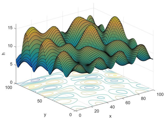
Figure 1.
Schematic diagram of planning space.
3.1.2. Trajectory Indication
The search for the optimal trajectory of the UAV is carried out in a three-dimensional space. A series of trajectory nodes need to be searched and selected in planning space, which is the basis composition of the trajectory.
Let be the trajectory nodes of the u-th trajectory, where represents the number of the trajectory nodes, and and denotes the start and target point, respectively. The line between two adjacent trajectory nodes is called the trajectory segment. Let , , ; then, the u-th trajectory can be represented as .
3.2. Uncertain Constraints in Trajectory Planning
It is necessary to factor in the threat areas and maneuverability in trajectory planning. The threat areas mainly include climate areas, radars, missiles and ground collision threats, while maneuverability mainly refers to the maximum flight distance, the maximum turning angle and other performance of the UAVs.
3.2.1. Uncertain Threat Areas
(1) Uncertain weather area
Complex weather conditions, which is the area that UAV has to avoid, will greatly affect the visibility of the UAV and at the same time weaken the efficiency of the infrared guidance system. Different weather regions with different characteristics reflect the need to build different models.
The area affected by thunderstorms and hail can be equivalent to a cylinder, the coordinate of the threat center is recorded as , and its influence radius is . Acoording to the past data, the threat radius can be considered as normal uncertain variables, that is, , and its uncertainty distribution
where and are real numbers with
Moreover, the area affected by fog and cloud can be reducible to a cube. According to the historical meteorological observations, it can be considered as a linear uncertain variable. Let be the coordinate of the threat center and be the threat side length, then , and its uncertainty distribution
where and are the maximum and minimum radius, respectively.
(2) Radar threat
Radar is the greatest detection threat of low-altitude penetration. Once the UAV is detected by the enemy’s radar, the UAV might be shot down by air defense weapons, so the detection coverage of radars should be avoided.
This paper assumes that radars are the same type of single-base pulse, and its detection ability is related to its maximum threat radius , which can be calculated as follows:
where is the transmitting power, and are the gains of the transmitting and receiving antennas, is the wave length of the transmitting wave, and is the average cross sectional area of the detection target. and are the feeder loss, is the receiver noise figure, k is the Boltzmann constant, T is the absolute temperature, is the receiver bandwidth, and is the detection terminal identification constant.
It can be seen from the Equation (23) that the influence radius of the radar is affected by many parameters, which is not constant due to the irresistible factors. Let be the radius of the radar; the parameters are usually relatively stable according to historical observation, so can be considered as a normal uncertain variable, that is, , and its uncertainty distribution
where denotes maximum threat radius of radar without the interference of uncertain factors and denotes the standard deviation.
3.2.2. Maneuverability
(1) Maximum flight distance
The maximum flight distance of the UAV is the flight distance with full fuel. Let be the maximum flight distance and N be the number of the trajectory nodes. Then, the constraint of the maximum flight distance can be established as follows:
where .
(2) Maximum turning angle
There are two main considerations for the constraint of the trajectory turning angle. On the one hand, due to the limitation of the maneuverability, the turning angle should not be too large; on the other hand, when the UAV is turning, the curvature needs to be considered to keep the trajectory at a safe distance from the terrain.
Let be the horizontal projection of the i-th trajectory segment, and the maximum turning angle is the angle between the vector and . Then, the constraint can be expressed as follows:
where denotes the length of the vector.
(3) Minimum trajectory segment distance
Frequent turning and detour flight is not desirable in order to improve the safety of the trajectory and reduce unjustified flight and fuel consumption; therefore, it is necessary to maintain a minimum flight distance before the UAV changes its direction. Let be the shortest trajectory segment, and then the constraint can be given as follows:
(4) Maximum climb/dive angle
This constraint limits the angle to climb and dive in the vertical direction, which ensures the UAV flight will be within a safe range. Let be the maximum climb/dive angle, then the angle between the vertical direction and the horizontal projection of the trajectory segment must satisfy the following constraint:
(5) Minimum flight altitude
A minimum flight altitude should be set to reduce the collision probability of UAVs and ground obstacles. Divide each trajectory segment into k equal parts, and store the trajectory height of each equipartition point into vector . Meanwhile, store the height of the grid corresponding to the equipartition point in the vector . Let be the minimum flight height of the UAV, and then the constraint can be expressed as follows:
(6) Approach angle of the target
In order to ensure the successful completion of specific targets, the UAV has to approach the target within a certain angle. Let and be the maximum and minimum allowable angles of the UAV to approach the target, respectively, then the constraint can be expressed as follows:
3.3. Objective Function of Trajectory Evaluation
Trajectory evaluation is crucially important in trajectory planning, which has to take various criterions into account. Generally speaking, three factors should be considered: fuel consumption, concealment and the threat degree.
3.3.1. Fuel Consumption
Fuel consumption refers to the total fuels consumed by the trajectory from the start point to the target point. The residence times decreases with the fuel consumption declining, which improves the security and saves the costs of the flight.
Let be the fuel consumption per unit distance. It is an uncertain variable influenced by various factors such as the flight speed and the temperature, and it is evenly distributed over a certain interval according to the historical data, so it is reasonable to be considered as a linear uncertain variable, that is, , and its uncertainty distribution is
where and are the maximum and minimum fuel consumption, respectively.
In addition, the UAV will be affected by other uncertain factors during the flight, resulting in additional fuel consumption . According to the observational data, this part of the fuel consumption , and its uncertainty distribution
where and are real numbers with .
Then, the objective function of fuel consumption can be calculated as follows:
3.3.2. Concealment
UAVs must maintain a certain flying height to ensure security. When UAVs fly at low altitudes, they are prone to collision with the terrian obstacles due to the inaccuracy of the control system. However, as the flight altitude increases, the UAV is more likely to be detected by the enemy, which results in the decreasing of security. Therefore, a relatively ideal trajectory should reduce the flight height of the UAV while ensuring its security.
What is more, the concealment of the trajectory is also affected by the average height of the planning space. Generally speaking, higher altitude of the planning space will lead to the worse concealment.
In this paper, the concealment degree given by domain experts is introduced to calculate the concealment of the trajectory, and is the concealment per unit elevation of the planning space, then the concealment of the trajectory can be expressed as follows:
where represents the average height of the planning space, and denotes the average altitude of the i-th trajectory segment, that is,
In trajectory planning, however, given by domain experts is affected by many unpredictable factors, and it is normally distributed around a certain value according to the historical observations, so it is reasonable to think it is a normal uncertain variable, that is, , and its uncertainty distribution is
Similarly, is considered as an exponential uncertain variable of parameter , that is, , and its uncertainty distribution is
where is real numbers with .
3.3.3. Threat Degree
In trajectory evaluation, the crucial issue is the calculation of the threat degree. According to Section 3.2.1, the trajectory threat degree mainly includes the impact of the weather and radar, and the security of the trajectory is proportional to the distance between the UAV and the threat center. The threat degree of the trajectory under the influence of different threat areas is calculated as follows.
(1) Threat degree of the weather
Weather areas are mainly divided into two main categories, one is the area posed by thunderstorms and hail areas, and the other is posed by fog and cloud areas. This section calculates the threat degree based on the mathematical models established for the two categories in Section 3.3.1.
The threat diagram of the thunderstorms and hail areas is shown in Figure 2, its threat degree to the UAV is inversely proportional to the distance between the UAV and threat area, and it is directly proportional to the radius of the area. Let be the threat degree of the UAV being threatened by the j-th thunderstorms and hail area at the position ; then, it can be expressed as follows:
where denotes the threat parameter of the j-th thunderstorms and hail area, is an uncertain variable denoting its threat radius, and represents the distance between the UAV and the center of the j-th threat area, which can be calculated as follows:
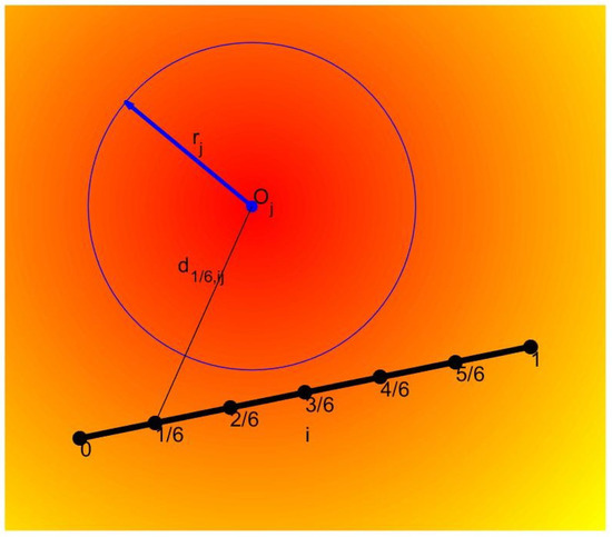
Figure 2.
Thunderstorms and hail area.
For the second uncertain weather, its threat degree is mainly related to the distance between the UAV and the center of the cube area and is also affected by its side length. It can be seen from Figure 3 that point A and point D are at the same distance from the center of the threat area, but it is obvious that point A is at the edge of the threat area while point D is out of it, so their threat degree is different. If the Euclidean distance is used in this case, we will conclude that the threat degree is the same, which is contrary to reality. Taking the particularity of the actual problem into account, an infinite norm is reasonable to define the distance between the trajectory and the areas, that is,
then the threat degree of the UAV being endangered by the j-th fog and cloud area can be calculated as follows:
where is an uncertain variable denoting the side length of the j-th area, denotes its threat parameter, and represents the distance between the current position of the UAV and the center of the j-th area.
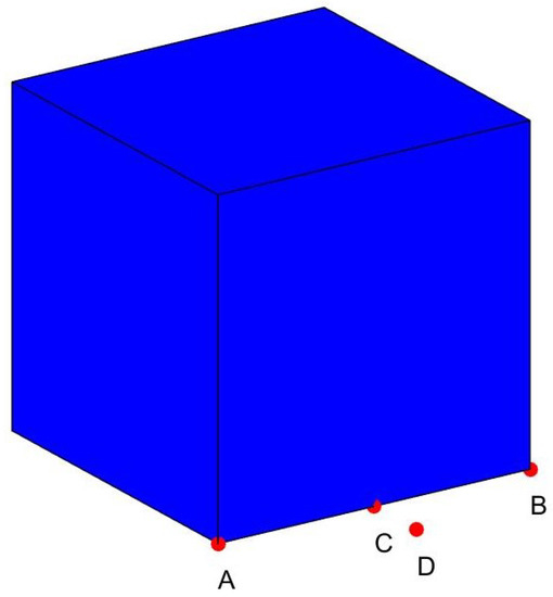
Figure 3.
Fog and cloud area.
(2) Radar threat areas
Threat degree of the radar to the UAV is inversely proportional to the fourth power of the distance between the UAV and the radar, and it is also related to the threat radius of the radar and its own parameters. Let be the threat degree of the UAV being threatened by the j-th radar at the position . It can be calculated as follows:
where denotes the distance between the UAV and the center of j-th radar, and is an uncertain variable representing the threat radius of the j-th threat source.
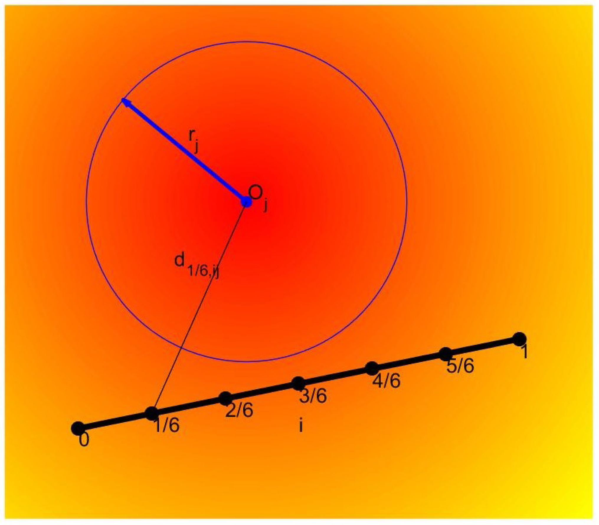
It is inevitable to integrate with respect to the u-th trajectory to accurately calculate the threat degree, which results in a heavy computation requirement. Therefore, the i-th trajectory segment is divided into six equal parts, and the threat degree can be obtained by calculating the average of the five equal points, that is,
where J denotes the number of threat areas, denotes the types of threat area, denotes the position of the equipartition point, which can be calculated as follows:
then, the threat degree of trajectory can be calculated by summing the threat degrees of different threat areas:
3.4. Uncertain Multi-Objective Trajectory Planning Model
Section 3.1 first analyzes the basic knowledge of the trajectory planning, and then the constraints are established, including the maximum flight distance, the maximum turning angle, the minimum flight altitude, etc. Finally, the evaluation criterions of the trajectory are given, which contain the fuel consumption, the concealment and the threat degree. Let be the feasible region; then, the uncertain multi-objective trajectory planning model (UMOTP) can be established as shown in Model 1.
| Model 1: UMOTP model |
Since there are uncertain variables and multiple objective functions in UMOTP, it is not a solvable mathematical model because a natural ordered relation in uncertain space does not exist, so the pareto efficient solution criterion that conforms to the actual problem will be used to transform the UMOTP problem into a deterministic multi-objective programming model.
4. Solution Method of UMOTP Problem
In Section 3, the UMOTP model is established; however, it is unable to obtain the optimal solution due to the existence of the uncertain variables, so the method of solving UMOTP problem will be introduced in this section.
For an uncertain objective function , the expected-value efficient trajectory to the UMOTP problem is a common solution method, which reflects the preference of long-term benefits. In trajectory planning, however, the stability of the trajectory should be taken into account as well.
Therefore, both the expected value and standard deviation of the fuel consumption, concealment and threat degree will be considered as the new objective function. Then, Model 1 can be transformed into the expected-value standard-deviation efficient trajectory to the uncertain multi-objective trajectory planning (-UMOTP) problem, as shown in Model 2.
| Model 2: -UMOTP model |
Remark 1.
Since the objective function involves uncertain vector , the results can only be optimal in some sense. Here, the -UMOTP model is to minimize both the expected value and standard deviation of the evaluation criterion. This policy is practical because it takes both the long-term benefits and volatility into consideration.
Definition 15.
Let ; then, the solution is called the expected-value standard-deviation efficient solution of the UMOTP problem if it is the Pareto efficient solution of the -UMOTP problem, that is, there does not exist such that
and
for at least one index .
The relation among the -UMOTP model, the E-UMOTP model and the -UMOTP model is transformed by Theorem 5.
Theorem 5.
Let and be the Pareto efficient trajectory set of the E-UMOTP and -UMOTP, respectively, and S be the Pareto efficient trajectory set of the -UMOTP. Then, we have .
Proof.
Let be both the efficient trajectory of the E-UMOTP and -UMOTP, that is,
Since is the efficient trajectory of E-UMOTP, there does not exist such that
and
for at least one index i. Similarly, there does not exist such that
and
for at least one index j.
It can be known that is the Pareto efficient trajectory of Model 2. Therefore, if is both the Pareto efficient trajectory of E-UMOTP and -UMOTP, then it is the Pareto efficient trajectory of -UMOTP, that is, if , then , so . □
In this paper, we assume that the uncertain variables are independent, then the expected value and standard deviation can be calculated according to Theorem 3 and Theorem 5. It is obvious that , , are strictly increasing with respect to , so all of them are uncertain variables according to Theorem 2. Let be the uncertainty distribution of , which can be calculated as follows:
after then, the expected value of can be obtained as follows:
and its standard deviation can be calculated according to Theorem 5 as follows:
Since the inverse uncertainty distribution of normal uncertain variable is
the uncertain distribution of the second objective can be calculated as follows:
and the expected value and standard deviation can be obtained as follows:
Similarly, the uncertainty distribution of can be calculated as follows:
Then, the expected value and standard deviation can be obtained as follows:
This section transforms the UMOTP problem into a sovable mathematical programming model. However, the Pareto front is difficult to solve due to the uncertain properties and the high degree of nonlinearity, so it is particularly important to design an efficient algorithm for solving multi-objective optimization.
5. Improved Particle Swarm Optimization for Multi-Objective Problem
In Section 4, the UMOTP problem is transformed into a solvable deterministic mathematical programming model. In this section, an efficient algorithm will be designed to solve the -UMOTP model. The ideas of non-dominated sorting and crowding distance in NSGA-II are introduced based on the PSO to improve the quality and maintain the diversity of the solution. Then, the improved constrained multi-objective backbones particle swarm optimization algorithm (BB-CMOPSO) is proposed and tested to verify the performance of the algorithm.
5.1. Algorithm Analysis
In order to deal with -UMOTP, an efficient optimization technique must be able to optimize the objective function under the constraints. This paper proposes a BB-CMOPSO algorithm, and the main works of this section are as follows:
(1) Consider both the degree of constraint violation and the Pareto dominance relation, and define a constrainted dominance to analyze the relation of the particles;
(2) Propose a new update method for the infeasible reserve set;
(3) In order to balance the global search and local development capabilities of the algorithm, a linear decline strategy is proposed to calculate the probability of choosing the global leader from the infeasible reserve set and the feasible reserve set.
5.1.1. Constrained Dominance
Consider the constrained violation degree and the Pareto dominance. The constrained dominance is introduced to analyze the relations between the particles and then update the individual leader and select particles into the feasible reserve set. Considering the particle , its constraint violation degree can be calculated as follows:
where and denote the equality and inequality constraints, respectively; is the allowable error for the violation of equality constraints; and S represents the current particle swarm. If , it means that the particle violates the j-th constraint.
After that, the constraint violation degree is used to evaluate each particle. For a given particle and , if they satisfy one of the following conditions: (1) ; (2) , while , and such that . Then, is said to constrained dominate .
5.1.2. Update the Individual Leader
The individual leader refers to the best position of the particle from initial to current iteration times, which can be updated based on the constrained dominance.
Let be the individual leader of the particle , if constrained dominates , ; if they do not dominate each other, randomly choose one from and as ; otherwise, .
5.1.3. Update the Feasible and Infeasible Reserve Sets
Two external reserve sets with fixed potential named infeasible and feasible reserve set will be designed to store the infeasible and non-inferior solutions, respectively, and the global leader will be selected from these two sets.
There are two purposes to search the feasible optimal solutions from the infeasible solutions: the first is that the diversity of the population can be improved by efficiently balancing feasible and infeasible solutions; the second is that the infeasible solution is used to explore the isolated feasible regions, which is able to search for better feasible solutions and is helpful to deal with the constrained programming problems with a small proportion of feasible solutions.
(1) Update the feasible reserve set
Pareto dominance is used to update the feasible reserve set as follows: Firstly, combine the particles in the feasible reserve set and new feasible solutions set into a new population. Then, select the particles that are not dominated by each other in the new population by using the Pareto dominance relation, and save them in the feasible reserve set. Finally, if the number of particles in the feasible reserve set exceeds its inherent capacity , then the particles will be filtered on the premise of maintaining the diversity of the solutions.
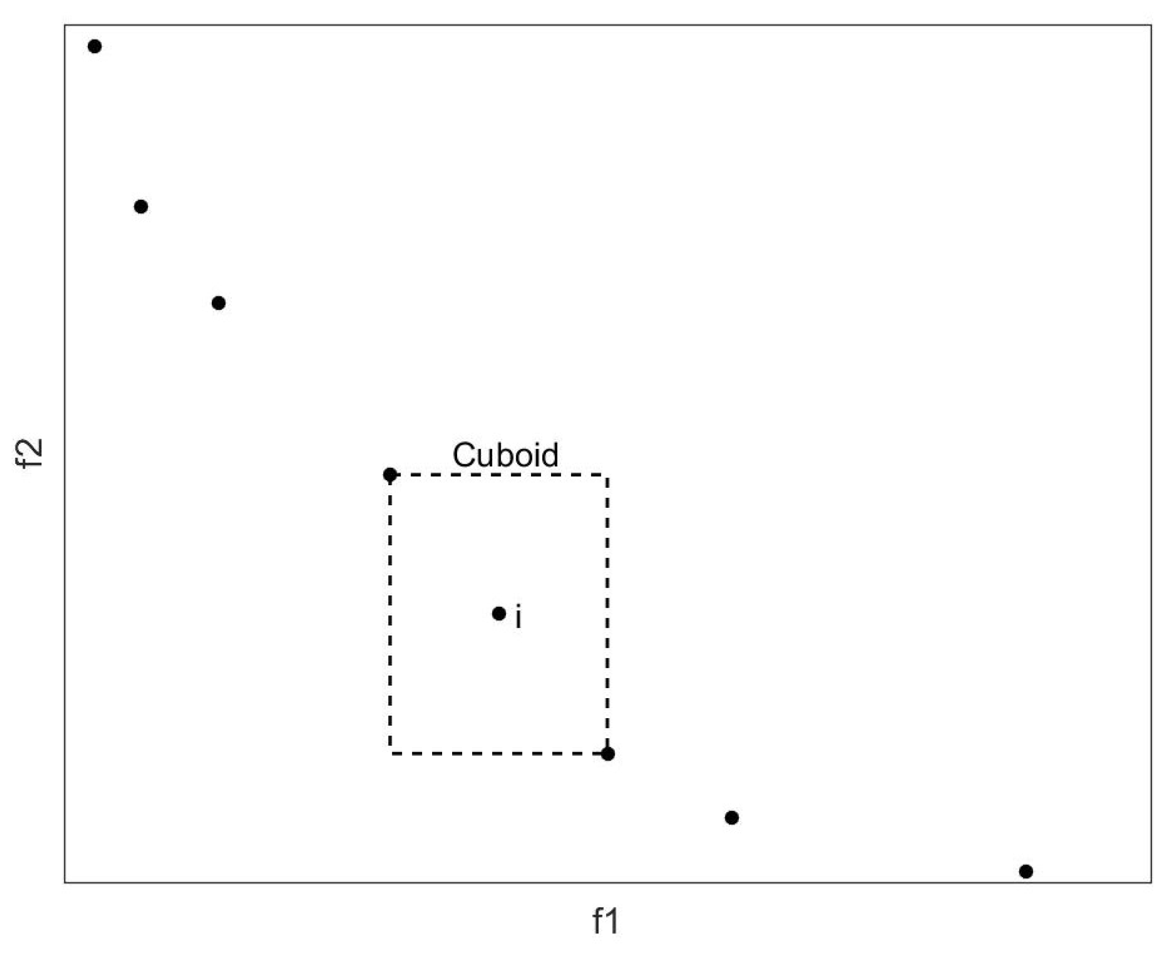
For this purpose, this paper calculates the crowding distance of each particle and retains the most sparsely distributed particles. As shown in Figure 4, the points represent the particles in the reserve set, and the crowding distance of the i-th particle is the average side length of the virtual quadrilateral. The boundary particles in each dimensional target space are given an infinite crowding distance to improve the ductility of the obtained Pareto front.
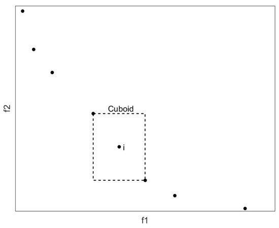
Figure 4.
Crowding distance.
(2) Update the infeasible reserve set
The infeasible reserve set can be refreshed based on the updated feasible reserve set. Firstly, combine the particles in the infeasible reserve set and the new infeasible solutions into a new population. Then, for a particle in new population, if one of the following conditions is satisfied, it will be saved in the infeasible reserve set: (a) there is a particle in the feasible reserve set that is dominated; (b) it is neither dominated by the particle in the feasible reserve set nor located in the sparse area. In order to determine whether a particle is in the sparse area, it will be put into the feasible reserve set, and if the crowding distance is times or more than the average crowding distance of the feasible reserve set, then the particle is considered to be located in the sparse area. Finally, if the particles stored in the infeasible reserve set exceed its inherent capacity , and then we calculate the crowding distance of each particle, and the particles with greater crowding distances will be retained.
Two classes of the infeasible solutions are preserved according to this method to update the infeasible reserve set. The former infeasible solution can increase the objective function value of the feasible solution, while the latter infeasible solution is beneficial to guide the particle exploring the undiscovered feasible regions.
5.1.4. Select the Global Leader
Since the infeasible solution can be considered as a bridge to guide particles to the isolated area, and it can guide particles to a feasible region when the feasible solution interval is small, then the diversity of the population can be improved. Therefore, selecting the particles in the infeasible reserve set as the global leader will enhance the global development capabilities; what is more, selecting the elements in the feasible reserve set as the global leader can also guide the particles to thoroughly develop the discovered feasible regions and further improve the quality of the existing feasible solutions.
This paper designs a dynamic allocation strategy based on selection probability to balance the two selection approaches; the global leader is selected from the infeasible reserve set and the feasible reserve set with probability and , respectively, which can be calculated as follows:
where denotes the algorithm iterations; and are constants satisfying .
There are two main advantages of this selection strategy:
(I) In the early stage of the algorithm, the global leader is chosen from the infeasible reserve set with a greater probability, which will contribute to maintain the diversity of the particles and enable them to search for more isolated feasible regions.
(II) As the number of iterations increases, the selection of the global leader gradually focuses on the feasible reserve set, which means that the algorithm will have more opportunities to search for feasible regions in later iterations so as to achieve the purpose of deeply exploring the feasible non-inferior solutions.
Remark 2.
If the infeasible reserve set is empty, global leader is chosed from the feasible reserve set; if the feasible reserve set is empty, the global leader is chosen from the infeasible reserve set.
After that, the global leader will be selected from the corresponding reserve set. In order to introduce a method for selecting the global leader, the angle of the particles is defined as follows.
Definition 16.
Considering two particles and , define
as the angle of particles and in the target space, where and denote the objective function value of the particle and , respectively.
The global leader is selected from the reserve set based on the angle between the particles. The specific method is as follows:
- (I)
- Calculate the angle between particle and each particle in reserve set S.
- (II)
- The particle is selected as the global leader if .
5.1.5. Update the Particle Position
Traditional particle swarm optimization relies on inertial weight and acceleration coefficient to balance the global exploration and local development. Experimental analysis, however, shows that the performance of the PSO is sensitive to these parameters, and there is not sufficient theory to draw up the guidelines of the parameter selection.
In order to overcome this problem, the backbones particle swarm optimization algorithm is proposed in [34]. A Gaussian distribution with respect to the global and individual leaders is used to update the particle position:
What is more, a new updating formula suitable for multi-objective programming problems based on the BBPSO is proposed in this paper:
where .
Compared with Equation (66), particle’s global leader , instead of its individual leader , is used in Equation (67). Similar to the crossover operator in evolutionary algorithms, this improvement will help particles build excellent modules with a faster speed. On the other hand, since the global leader is randomly selected from the external reserve set containing several particles, the development of the global leader with the probability of 50% will not destroy its diversity. In addition, when , the gravitational factor in Equation (66) becomes the combination of the global leader and individual leader with random weights, which further expands the search scope.
5.1.6. Time-Varying Variation
The advantage of the PSO is its fast convergence speed. However, it is precisely because of its fast convergence that the multi-objective programming based on PSO algorithm may prematurely converge to the local Pareto front.
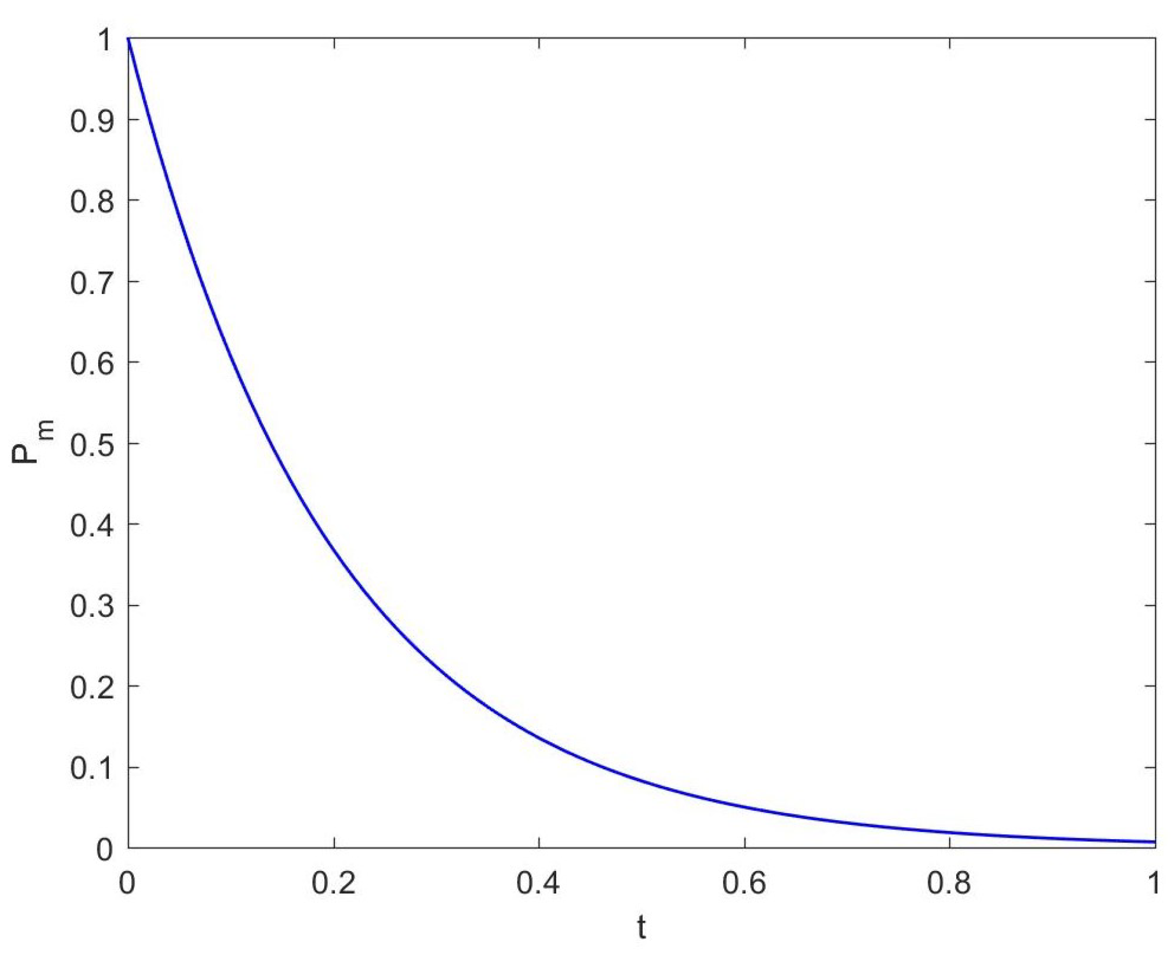
A time-varying mutation operator is proposed to avoid the premature convergence, and the mutation parameter is used to calculate the mutation probability and the range of movement of the particle land when the mutation is executed. The pseudo code of time-varying mutation is shown in Algorithm 1, the variation curve of the mutation probability with is shown in Figure 5.
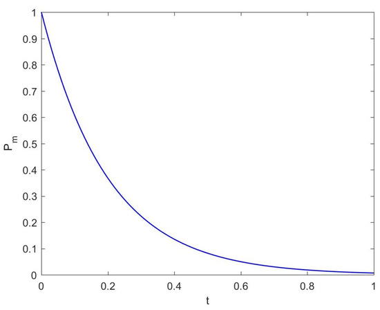
Figure 5.
Mutation probability curve.
It can be seen from Figure 5 that in the early stage, most of the particles will be affected by the mutation operator, and each particle is allowed to mutate throughout the decision space, so the global exploration ability is excellent. As the number of iterations increases, the influence of the mutation operator gradually weakens, which is not only reflected in the decrease in mutation probability, but also in the gradually shrinking variation range of particles; then, the algorithm will have a better local development.
Remark 3.
If the mutated particle exceeds its allowable range, the boundary is taken as its new position.
| Algorithm 1 Pseudo code of time-varying mutation |
|
5.2. Algorithm Design
The relevant theories of constrained multi-objective particle swarm algorithm are analyzed in Section 5.1, and the algorithm can be designed as follows:
Step 1. Set the parameters of the algorithm, including the number of particles M, the potential of the feasible and infeasible reserve set and , the iterations T and mutation parameter .
Step 2., initialize the particle swarm. Each particle is randomly assigned an initial position in the feasible region; the individual leader of each particle is set as itself; the feasible reserve set and the infeasible reserve set are both set to empty.
Step 3. Calculate the fitness and constraint violation degree of the particles.
Step 4. Divide the particles into two categories: feasible and infeasible solutions, and the method proposed in Section 5.1.2 is used to update the feasible and infeasible reserve set.
Step 5. If the termination condition is satisfied, the algorithm stops; otherwise, perform the following steps.
Step 6. Perform the following operations for each particle in sequence:
(1) Select its global leader from the infeasible reserves with probability according to the method in Section 5.1.4;
(2) Update its individual leader using the method mentioned in Section 5.1.2;
(3) A new particle position is regenerated by Equation (67);
(4) Perform time-varying mutation according to the method in Section 5.1.6.
Step 7., transfer to Step 3.
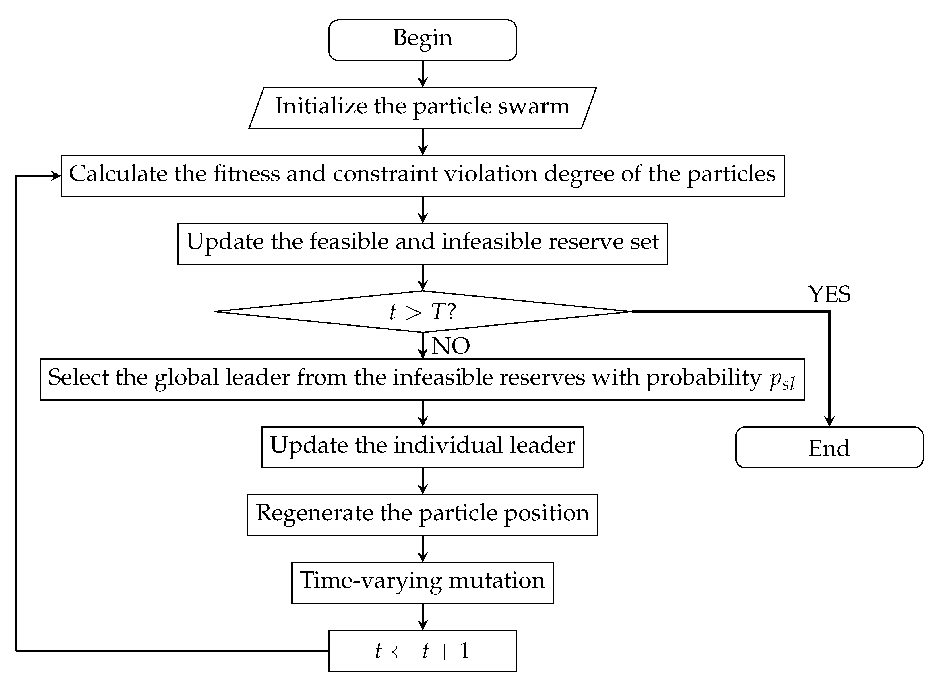
The flow diagram of the algorithm is shown in Figure 6.

Figure 6.
Flow diagram of the BB-CMOPSO.
5.3. Algorithm Test
This section will analyze the performance of the improved BB-CMOPSO, and two typical test functions are used to verify the effectiveness of the algorithm.
5.3.1. Test Functions
Two typical test functions are selected in this experiment: BNH [35] and OSY [36], which are all minimization problems. The feasible rates of BNH and OSY are 3.16% and 3.25%, respectively, and a small feasible rate will challenge the algorithm’s ability to search for feasible solutions.
Test function 1: OSY
Test function 2: BNH
5.3.2. Performance Indicators
In order to quantitatively analyze the performance of a multi-objective algorithm, two aspects should be taken into consideration: (1) the distance between the Pareto front generated by our algorithm and the real Pareto front; (2) the distribution of the solutions. Therefore, two concepts are defined as follows:
Definition 17. (Spacing)
Spacing defined as follows is used to measure the distribution of the obtained non-inferior solution set in the target space:
where
where denote the number of the obtained non-inferior and objective function, respectively. It is obvious that the obtained non-inferior solutions are uniformly distributed in the solution space if and only if .
Definition 18. (Generational distance)
Generational distance defined as follows is used to measure the distance between the obtained non-inferior solution set and the real Pareto front:
where denotes the minimum Euclidean distance between the element i in the non-inferior solution set and the element in the Pareto front. If , then the obtained non-inferior solutions are all located on the Pareto front.
5.3.3. Test Results and Comparison
In order to understand how competitive the BB-CMOPSO is, we compare it with two state-of-the-art multi-objective evolutionary algorithms: Nondominated Sorting Genetic Algorithm II (NSGA-II) and HBGA.
For each test function, the algorithms will run 30 times independently, and the initial population is set at the same potential. The statistical results of the three algorithms on the SP and GD measures are shown in Table 1.

Table 1.
Comparison of the GD and SP.
It can be known from the table that for both the function BNH and OSY, the BB-CMOPSO algorithm achieves the best average GD and SP, which means that its optimal solution set is closest to the real Pareto front, and in terms of the distribution, it is much better than NSGA-II and HBGA. Therefore, the BB-CMOPSO is an efficient method to deal with CMOTP problems.
6. Computational Results
Section 3, Section 4 and Section 5 establish the UMOTP model and design and test an improved BB-CMOPSO algorithm. This section will use the algorithm to conduct simulation experiments on UMOTP problem.
In this experiment, a simulation experiment is carried out on MATLAB, and the relevant experimental parameters are set as follows:
(1) Maneuverability of UAV
The parameters are set as shown in Table 2 according to the practical investigation of the maneuverability of a series UAVs.
Table 2.
Maneuverability of UAV.
(2) Parameters of threat areas
The parameters of the threat area in this experiment are set as shown in Table 3 based on the analysis of the threat areas in Section 3.3.2 and combination with the actual battlefield environment.
Table 3.
Parameters of threat areas.
(3) Experimental parameters
• Number of trajectory nodes ;
• Number of particles ;
• Potential of the feasible and infeasible reserve set ;
• Variation parameter ;
•.
(4) Uncertain variable parameters
Based on the historical data and uncertain statistics, the parameters of uncertain variables are set as follows:
• Fuel consumption per unit distance is a linear uncertain variable; let . Fuel consumption produced by other uncertain factors is a lognormal uncertain variable; let .
• Concealment decreased by the rising unit height is a normal uncertain variable; let . Threat cost per unit height of the average elevation increase in the planned area follows a exponential distribution; let .
• Threat radius in the area of thunderstorm and hail is a normal uncertain variable; let ;
• Side length of the area affected by fog and larger cloud can be considered as a linear uncertain variable; let ;
• Threat radius is reasonable to be considered as a normal variable; let .
Therefore, the -UMOTP model can be transformed into a mathematical model as shown in Model 3, and some Pareto efficient solutions of the uncertain trajectory planning model are shown in Table 4.
Table 4.
Some Pareto efficient solutions for uncertain trajectory planning.
The experimental data in Table 4 show that different objective functions of the trajectory planning mathematical model restrict each other, which is mainly reflected in two aspects. One is the mutual restriction between different evaluation criterions. For example, the fuel consumption of trajectory 7 is more than trajectory 5, but its threat degree is smaller; the fuel consumption of trajectory 4 is smaller, but its threat degree is greater; the concealment of trajectory 9 is lower, but its fuel consumption is higher than some trajectories. The second is the contradiction between the expected value and standard deviation of the same evaluation indicator. For example, the expected value of the threat degree of trajectory 4 is smaller than trajectory 1, but its volatility is greater, that is, the stability is not ideal.
It can be learned from Table 4 that the efficient trajectories are contradictory, and there is no single trajectory that minimizes all the objective functions, so there is no absolute optimal trajectory. If decision-makers hope for the lowest threat degree, they have to sacrifice the fuel consumption to avoid the threat areas. Similarly, if the decision-maker wants to complete the combat mission as soon as possible, they may be threatened. Therefore, different optimal trajectories will be defined under the different combat mission.
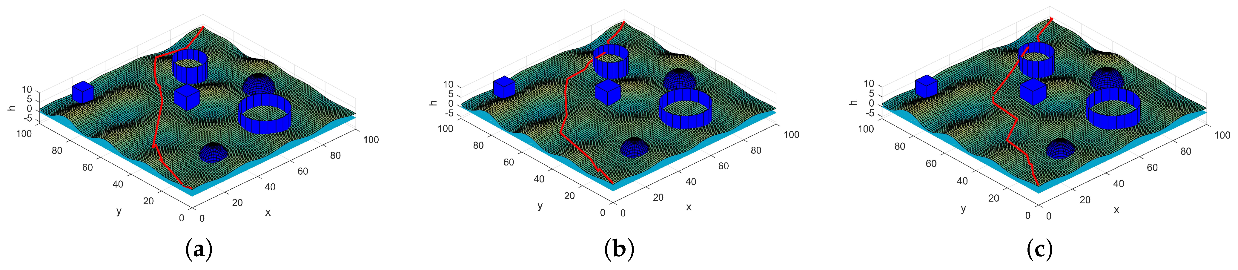
In trajectory planning, there are usually two strategies for decision-makers to determine the optimal trajectory under the different combat missions. One is to assign different weights to each objective function under specific conditions; the second is to limit some objections and then find the optimal value of the remaining targets under this condition. The optimal trajectories obtained by these two methods are shown in Figure 7 and Figure 8, respectively.
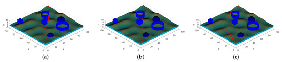
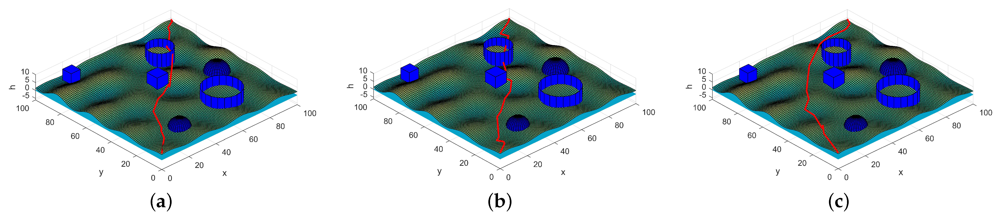
Figure 7.
Optimal trajectory under different weights. (a) = (0.5,0.1,0.1,0.1,0.1,0.1), which means the decision-maker hopes that the fuel consumption is as low as possible. (b) = (0.1,0.1,0.5,0.1,0.1,0.1), which means the decision-maker hopes that the trajectory is more concealed. (c) = (0.1,0.1,0.1,0.1,0.5,0.1), which means the decision-maker hopes that the threat degree is as low as possible.
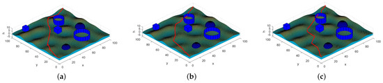
Figure 8.
Optimal trajectory under different preconditions. (a) Least threat degree with fuel consumption and concealment not exceeding 1000 and 500, respectively. (b) Least fuel consumption with threat degree and concealment not exceeding 900 and 500, respectively. (c) Best concealment with fuel consumption and threat degree not exceeding 970 and 1000, respectively.
In Figure 7, different weights are applied to the objective function according to combat mission. The value of the weight indicates the preference degree of the criterion, and the optimal solution under different circumstances is obtained. For example, in a certain task, where UAVs have to achieve the mission as quickly as possible and are willing to take some risks, the weight = (0.5, 0.1, 0.1, 0.1, 0.1, 0.1) can be set to obtain the trajectory as shown in Figure 7a. The adaptive value of this trajectory after normalization under this weight is 0.148. Similarly, decision-makers can change the weights according to the actual environment and combat requirements to obtain the corresponding optimal trajectory.
Continuing to analyze Figure 1, we can find it visually that if the decision-maker pays more attention to fuel consumption (as shown in Figure 7a), the trajectory distance obtained is shorter, but it will cross the threat area with a greater probability, and the trajectory is more dangerous; if the decision-makers focus more on a smaller threat degree, the trajectory distance and fuel consumption will increase.
The decision-maker can also set the preconditions that the trajectory needs to satisfy according to the combat mission and then select the optimal trajectory that satisfies the conditions. Assuming that in a certain flight mission, the fuel consumption should not exceed 1000, and the altitude cost must not exceed 500, then the trajectory with the smallest threat coefficient is selected on this basis, and the trajectory shown in Figure 8a is obtained.
What is more, the optimal trajectory obtained by the linear weighting, ideal point method and minimax method are the part of the Pareto front of the -UMOTP model, which only represents the best decision under a certain preference, so it is not universal. The BB-CMOPSO algorithm is used in this section to solve the -UMOTP model and the optimal trajectory set is obtained, then the optimal trajectory under different preference is analyzed, which provides a decision-making scheme for trajectory planning under different combat missions, and the shortcomings of the traditional method are overcome.
7. Conclusions
This paper first proposed the uncertain multi-objective trajectory planning based on uncertainty theory in a complex environment with asymmetric information. Since it can only be optimal in some sense under the state of indeterminacy, the concept of the expected-standard-deviation efficient trajectory was defined. Simulation modeling is carried out for the planned space; then, the constraint conditions of the flight trajectory are analyzed; and finally, the uncertain flight trajectory planning model is established by comprehensive evaluation of the UAV from three aspects. Compared with probabilistic methods, the uncertain UAV trajectory planning model with expert reliability established in this paper is more suitable for combat planning in uncertain environments. In order to effectively solve the UMOTP problem, this paper designs an improved backbones multi-objective particle swarm algorithm based on the NSGA-II and PSO algorithm and has achieved good performance.
Author Contributions
Conceptualization, A.Z. and M.Z.; methodology, A.Z.; software, A.Z. and H.Z.; validation, B.L. and H.Z.; writing—original draft preparation, A.Z.; writing—review and editing, B.L., M.Z. and H.Z. All authors have read and agreed to the published version of the manuscript.
Funding
This research was funded by National Natural Science Foundation of China grant number No.11801564.
Conflicts of Interest
The authors declare no conflict of interest.
References
- Dijkstra, E.W. A note on two problems in connexion with graphs. Numer. Math. 1959, 1, 269–271. [Google Scholar] [CrossRef] [Green Version]
- Hart, P.E.; Nilsson, N.J.; Raphael, B. A Formal Basis for the Heuristic Determination of Minimum Cost Paths. IEEE Trans. Syst. Sci. Cybern. 1972, 4, 28–29. [Google Scholar] [CrossRef]
- Khatib, O. Real-Time Obstacle Avoidance System for Manipulators and Mobile Robots. Int. J. Robot. Res. 1986, 5, 90–98. [Google Scholar] [CrossRef]
- Kavraki, L.E.; Svestka, P.; Latombe, J.C.; Overmars, M.H. Probabilistic roadmaps for path planning in high-dimensional configuration spaces. IEEE Trans. Robot. Autom. 1996, 12, 566–580. [Google Scholar] [CrossRef] [Green Version]
- Roberge, V.; Tarbouchi, M.; Labonté, G. Comparison of Parallel Genetic Algorithm and Particle Swarm Optimization for Real-Time UAV Path Planning. Ind. Inform. IEEE Trans. 2013, 9, 132–141. [Google Scholar] [CrossRef]
- Venegas, G.; Samaniego, F.; Girbes, V.; Armesto, L.; Garcia-Nieto, S. Smooth 3D path planning for non-holonomic UAVs. In Proceedings of the 2018 7th International conference on Systems and Control (ICSC), Valencia, Spain, 24–26 October 2018; pp. 1–6. [Google Scholar]
- Jun, M.; D’Andrea, R. Path Planning for Unmanned Aerial Vehicles in Uncertain and Adversarial Environments. In Cooperative Control: Models, Applications and Algorithms; Butenko, S., Murphey, R., Pardalos, P.M., Eds.; Springer: Boston, MA, USA, 2003; pp. 95–110. [Google Scholar]
- Marinakis, Y.; Marinaki, M. A Hybrid Multi-Swarm Particle Swarm Optimization algorithm for the Probabilistic Traveling Salesman Problem. Comput. Oper. Res. 2010, 37, 432–442. [Google Scholar] [CrossRef]
- Allahviranloo, M.; Chow, J.; Recher, W.W. Selective vehicle routing problems under uncertainty without recourse. Transp. Res. Part Logist. Transp. Rev. 2014, 62, 68–88. [Google Scholar] [CrossRef]
- Aoude, G.S.; Luders, B.D.; Joseph, J.M.; Roy, N.; How, J.P. Probabilistically safe motion planning to avoid dynamic obstacles with uncertain motion patterns. Auton. Robot. 2013, 35, 51–76. [Google Scholar] [CrossRef]
- Stentz, A. The focused D* Algorithm for RealTime Replanning. Int. Jt. Conf. Artif. Intellgence 1995, 1652–1659. [Google Scholar]
- Yu, X.Y.; Fan, Z.Y.; Ou, L.L.; Zhu, F.; Guo, Y.K. Optimal Path Planning Satisfying Complex Task Requirement in Uncertain Environment. Robotica 2019, 37, 1956–1970. [Google Scholar] [CrossRef]
- Tavoosi, V.; Marzbanrad, J.; Golnavaz, M. Optimized path planning of an unmanned vehicle in an unknown environment using the PSO algorithm. IOP Conf. Ser. Mater. Sci. Eng. 2020, 671, 012009. [Google Scholar] [CrossRef]
- Liu, B. Uncertainty Theory, 2nd ed.; Springer: Berlin, Germany, 2007. [Google Scholar]
- Liu, B. Uncertainty Theory: A Branch of Mathematics for Modeling Human Uncertainty; Springer: Berlin, Germany, 2010. [Google Scholar]
- Chen, B.; Liu, Y.; Zhou, T. An entropy based solid transportation problem in uncertain environment. J. Ambient. Intell. Humaniz. Comput. 2019, 10, 357–363. [Google Scholar] [CrossRef]
- Zhu, K.; Shen, J.; Yao, X. A three-echelon supply chain with asymmetric information under uncertainty. J. Ambient. Intell. Humaniz. Comput. 2017, 152, 66–80. [Google Scholar] [CrossRef]
- Salehpoor, I.B.; Molla-Alizadeh-Zavardehi, S. A constrained portfolio selection model at considering risk-adjusted measure by using hybrid meta-heuristic algorithms. Appl. Soft Comput. 2019, 75, 233–253. [Google Scholar] [CrossRef]
- Liu, B. Theory and Practice of Uncertain Programming, 2nd ed.; Springer: Berlin, Germany, 2009. [Google Scholar]
- Liu, B.; Chen, X. Uncertain Multiobjective Programming and Uncertain Goal Programming. J. Uncertianty Anal. Appl. 2015, 3, 10. [Google Scholar] [CrossRef] [Green Version]
- Zheng, M.; Yi, Y.; Wang, Z.; Liao, T. Efficient solution concepts and their application in uncertain multiobjective programming. Appl. Soft Comput. 2017, 56, 557–569. [Google Scholar] [CrossRef]
- Zheng, M.; Yi, Y.; Wang, Z.; Liao, T. Relations among efficient solutions in uncertain multiobjective programming. Fuzzy Optim. Decis. Mak. 2017, 16, 329–357. [Google Scholar] [CrossRef]
- Zheng, M.; Yuan, Y.; Wang, X.; Wang, J.; Mao, S. The information value and the uncertainties in two-stage uncertain programming with recourse. Soft Comput. 2018, 22, 5791–5801. [Google Scholar] [CrossRef]
- Wang, Z.; Guo, J.; Zheng, M.; Wang, Y. Uncertain multiobjective traveling salesman problem. Eur. J. Oper. Res. 2017, 241, 478–489. [Google Scholar] [CrossRef] [Green Version]
- Wang, J.; Guo, J.; Zheng, M.; Wang, Z.; Li, Z. Uncertain multiobjective orienteering problem and its application to UAV reconnaissance mission planning. J. Intell. Fuzzy Syst. 2018, 34, 2287–2299. [Google Scholar] [CrossRef]
- Guo, J.; Wang, Z.; Zheng, M.; Wang, Y. Uncertain multiobjective redundancy allocation problem of repairable systems based on artificial bee colony algorithm. Chin. J. Aeronaut. 2014, 27, 1477–1487. [Google Scholar] [CrossRef] [Green Version]
- Schaffer, J.D. Multiple objective optimization with vector evaluated genetic algorithms. In Proceedings of the First International Conference on Genetic Algorithms and Their Applications, Pittsburg, PA, USA, 24–26 July 1985; pp. 93–100. [Google Scholar]
- Goldberg, D.E.; Korb, B.; Deb, K. Messy Genetic Algorithms: Motivation, Analysis, and First Results. Complex Syst. 1989, 3, 493–530. [Google Scholar]
- Srinivas, N.; Deb, K. Multiobjective Function Optimization Using Nondominated Sorting Genetic Algorithms. Evol. Comput. 1994, 2, 1301–1308. [Google Scholar] [CrossRef]
- Deb, K.; Agrawal, S.; Pratap, A.; Meyarivan, T. A Fast Elitist Non-dominated Sorting Genetic Algorithm for Multi-objective Optimization: NSGA-II. In International Conference on Parallel Problem Solving from Nature; Springer: Berlin/Heidelberg, Germany, 2000; pp. 849–858. [Google Scholar]
- Deb, K.; Jain, H. An Evolutionary Many-Objective Optimization Algorithm Using Reference-Point-Based Nondominated Sorting Approach, Part I: Solving Problems With Box Constraints. IEEE Trans. Evol. Comput. 2014, 18, 577–601. [Google Scholar] [CrossRef]
- Liu, B. Some research problems in uncertainty theory. J. Uncertain Syst. 2009, 3, 3–10. [Google Scholar]
- Yao, K. A formula to calculate the variance of uncertain variable. Soft Comput. 2015, 19, 2947–2953. [Google Scholar] [CrossRef]
- Kennedy, J. Bare bones particle swarms. In Proceedings of the 2003 IEEE Swarm Intelligence Symposium, Indianapolis, Indiana, 24–26 April 2003; pp. 80–87. [Google Scholar]
- Binh, T.T.; Korn, U. MOBES: A multiobjective evolution strategy for constrained optimization problems. Proc. 3rd Int. Conf. Genet. Algorithms 1997, 25, 27. [Google Scholar]
- Osyczka, A.; Kundu, S. A new method to solve generalized multicriteria optimization problems using the simple genetic algorithm. Struct. Optim. 1995, 10, 94–99. [Google Scholar] [CrossRef]


Publisher’s Note: MDPI stays neutral with regard to jurisdictional claims in published maps and institutional affiliations. |
© 2021 by the authors. Licensee MDPI, Basel, Switzerland. This article is an open access article distributed under the terms and conditions of the Creative Commons Attribution (CC BY) license (https://creativecommons.org/licenses/by/4.0/).