Article

Principal Component Wavelet Networks for Solving Linear Inverse Problems

by
Bernard Tiddeman
1,* and
Morteza Ghahremani
2
1
Department of Computer Science, Aberystwyth University, Aberystwyth SY23 3DB, UK
2
A.I. Virtanen Institute for Molecular Sciences, University of Eastern Finland, 70150 Kuopio, Finland
*
Author to whom correspondence should be addressed.
Symmetry 2021, 13(6), 1083; https://doi.org/10.3390/sym13061083
Submission received: 18 February 2021 / Revised: 31 May 2021 / Accepted: 1 June 2021 / Published: 17 June 2021
(This article belongs to the Special Issue Symmetry in Vision II)

Abstract

:
In this paper we propose a novel learning-based wavelet transform and demonstrate its utility as a representation in solving a number of linear inverse problems—these are asymmetric problems, where the forward problem is easy to solve, but the inverse is difficult and often ill-posed. The wavelet decomposition is comprised of the application of an invertible 2D wavelet filter-bank comprising symmetric and anti-symmetric filters, in combination with a set of 1 × 1 convolution filters learnt from Principal Component Analysis (PCA). The 1 × 1 filters are needed to control the size of the decomposition. We show that the application of PCA across wavelet subbands in this way produces an architecture equivalent to a separable Convolutional Neural Network (CNN), with the principal components forming the 1 × 1 filters and the subtraction of the mean forming the bias terms. The use of an invertible filter bank and (approximately) invertible PCA allows us to create a deep autoencoder very simply, and avoids issues of overfitting. We investigate the construction and learning of such networks, and their application to linear inverse problems via the Alternating Direction of Multipliers Method (ADMM). We use our network as a drop-in replacement for traditional discrete wavelet transform, using wavelet shrinkage as the projection operator. The results show good potential on a number of inverse problems such as compressive sensing, in-painting, denoising and super-resolution, and significantly close the performance gap with Generative Adversarial Network (GAN)-based methods.

1. Introduction

Linear inverse problems occur frequently in image processing applications. These are asymmetrical problems, in which the forward solution is well defined and straightforward to compute, but the inverse problem is often ill-posed and difficult to compute. The goal is to estimate an underlying (uncorrupted) signal x , given a set of noisy measurements y , with noise n that have undergone some known linear transformation A i.e.,
y = A x + n .
One standard approach to solving such problems, which are typically ill-posed, involves regularising the problem using a signal prior ϕ ( x ) i.e.,
argmin x 1 2 | | y A x | | 2 2 + λ ϕ ( x ) ,
where λ is a non-negative weighting term. Generally the signal prior is intended to encourage sparsity of x in some basis, such as a wavelet domain [1,2,3,4,5]. Such hand designed priors have certain advantages, for example they form a convex optimisation problem with global optimality, and provide various theoretical guarantees. Unfortunately such priors are often too generic to constrain the problem, and can result in noise like images or other artefacts.
In this paper, we first explore previous work related to solving linear inverse problems, and possible image representations that could help to support their solution. Then we introduce the Principal Component Wavelet Networks, and demonstrate that this relatively simple approach can produce results that are comparable to the state-of-the-art, with a fixed training cost and are robust to over-fitting.

2. Literature Review

2.1. Deep Learning Based Techniques

To overcome the disadvantages of hand-crafted features, several learning based methods have been proposed. Most of these are designed for specific purposes, such as inpainting [6], image denoising/structured recovery [7], compressive sensing [8], super resolution [9,10] and deblurring [11]. Recently adversarial learning with deep neural networks has been applied to many of these problems with impressive results. OneNet is a particular example designed to solve such linear inverse problems in general [12]. OneNet combines a classifier with an auto-encoder, which is trained to project perturbed images back to their ground truth, and to classify perturbed/unperturbed images. The network is used as the projection operator in an alternating direction method of multipliers (ADMM) based technique. They demonstrated good results on a number of inverse problems. The training of the projection operator uses two discriminator networks (in the latent and image spaces) to distinguish perturbed from unperturbed images. They alternate training of the projection operator (to project “fake” unperturbed images into the space of unperturbed images) with training of the discriminator (to detect projected images from original, unperturbed images). Hence it is a form of Generative Adversarial Network (GAN).
GANs are known to be challenging to train [13,14], as they are prone to local minima, and are sensitive to the perturbations introduced in the training phase. Recently, various approaches have been proposed to speed up the optimisation using projection-based operators. Differential unrolled ADMM (DU-ADMM) has been proposed [15], which improves on the original OneNet, showing faster convergence and a reduction in overfitting during training. In a similar vein, Reference [16] used projected gradient descent (PGD) to allow a significant speed up in the convergence, by removing the need to compute the Jacobian of the gradient. Nevertheless, the training still requires generating artificial perturbed images, which the system learns to project back into the original so could be prone to bias due to the choice of perturbations. The system also requires learning many layers and parameters, which could lead to overfitting.
In this paper we show that a much simpler system can achieve results that improve on the original OneNet results in the majority of experiments, and improve on DU-ADMM on 3 tasks out of 8, with an unsupervised deterministic learning algorithm and very short training times. It is important to note that we use a “traditional” soft-thresholding projection operator, rather than a deep learning/GAN-based projection operator. We simply learn a more suitable wavelet decomposition for representing the dataset. As such, this work bridges the gap between traditional approaches and GAN-based approaches, and raises important questions relating to the relative importance of algorithm choice vs data representation.

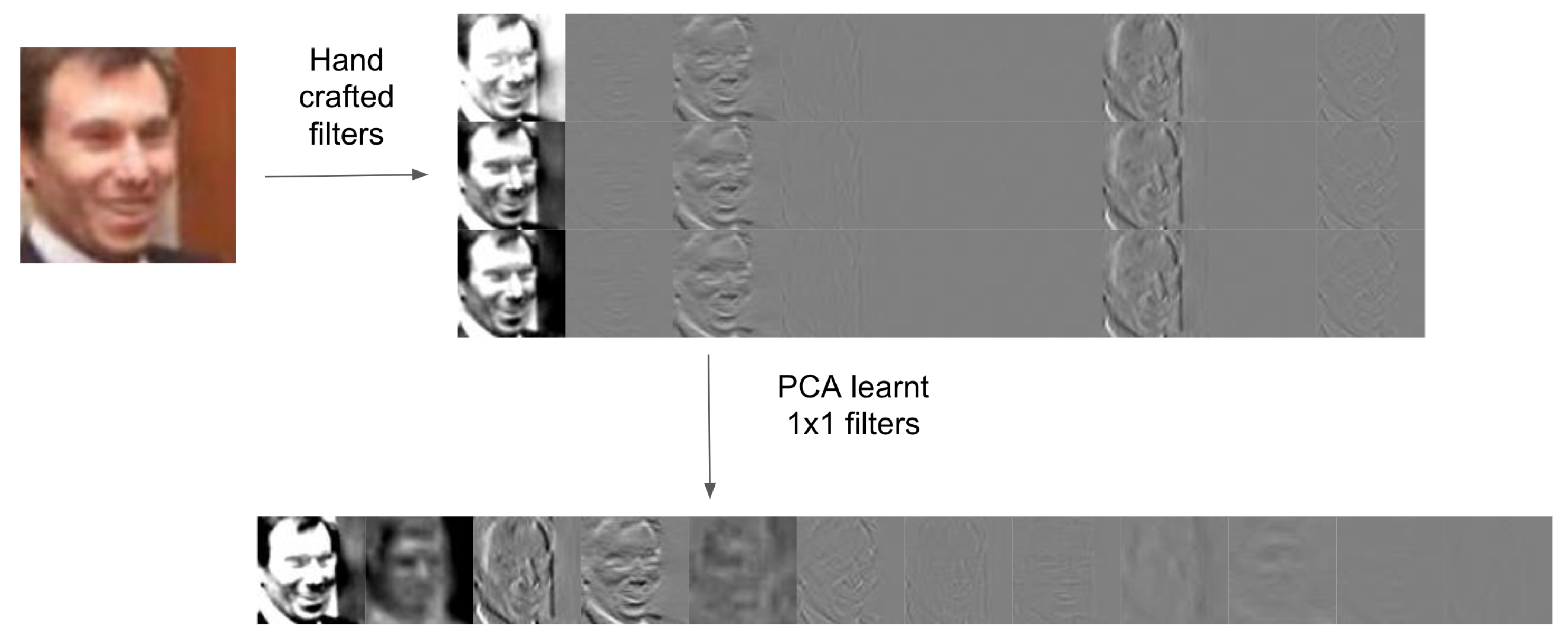
2.2. Image Representations

An appropriate image representation can be important to the success of an algorithm. Various image representations exist, such as the spatial and Fourier domain, various wavelet domain representations (such as continuous and discrete) and scattering wavelets, among others. Other representations are less explicit, but exist nevertheless, such as in Deep CNNs in the intermediate stages of auto-encoder networks.
Wavelet transforms generally filter an image with multiple versions of a single “mother” wavelet function that has been dilated and rotated in multiple directions. The wavelet subbands and/or low-pass filtered image may be kept at full resolution [17], or subsampled, typically by powers of 2 in x and y e.g., [18]. Decimation of both the low-pass and high pass filtered images provides a compact representation, but is known to lead to artefacts in the reconstruction. Various over-complete wavelet bases (or wavelet frames) have been proposed previously, such as double-density wavelets [19], dual-tree wavelets [20] or a combination of both [21]. The disadvantage of using a highly redundant representation is that it grows in size exponentially with the depth of the network.
Convolutional Neural Networks (CNNs) follow a similar pattern, but with some notable differences, including:
  • The filters are learnt from the data, rather than hard coded, usually by a back-propagation algorithm.
  • The number of filters is generally much larger than in wavelet analysis.
  • The high-pass subbands are themselves subjected to further rounds of filtering.
  • Non-linear components are generally introduced, such as ReLU activation functions and max pooling operators.
  • Inversion generally requires the training of a separate decoder network, although reversible networks do exist [22].
Scattering networks are another approach to bridging the gap between CNNs and wavelet analysis [23]. In scattering networks a set of oriented complex Mortlet wavelets of different scales are applied to the image, then the complex magnitude of the resulting subbands is found. The process can be repeated on these in a hierarchy. Finally the magnitude subbands of all levels are smoothed and subsampled to represent the image. The resulting representation has good shift and rotation invariance. One disadvantage of scattering networks for the proposed application to linear inverse problems, is the lack of a simple, direct, inversion algorithm. Scattering networks have been inverted by direct optimisation [24], by learning a reconstructing generative network [25] and by a hybrid algorithm [24]. The generative network approach appears the most promising from the perspective of solving linear inverse problems, but the reconstruction results exhibit some artefacts, and they haven’t yet been evaluated for solving linear inverse problems of the type described here.
Various combinations of wavelet analysis and PCA have been proposed previously, but not the particular structure proposed here. The application of PCA to (decimated) wavelet transforms has been used frequently e.g., [26,27,28]. In those examples, PCA is applied to the whole wavelet transformed image (after suitable scaling of the subbands) or to each subband independently, so for the purposes of PCA each image or subband constitutes a ‘point’ in the high dimensional space to which PCA is applied. In this work, PCA is applied to ‘fibres’ in the partially decomposed space i.e., the values across channels at a particular 2D location. Performing PCA in this way produces a decomposition algorithm identical in structure to convolutional neural networks, where the mean subtraction becomes the bias and the 2D convolutional filters are a linear combination of the selected wavelet filters. Given the success of CNNs in solving a wide range of problems, we believe it is informative to consider different learning algorithms within the successful CNN structure.
PCANet is another related approach, used to create 2D filters by applying PCA to overlapping patches extracted from the training images [29,30]. In this approach, the extracted patches first have the mean removed and PCA is applied to the resulting image stack to learn convolutional filters corresponding to the first N principal components. The process can be repeated on each of the resulting subbands in a hierarchy. When combined with binary hashing and blockwise histograms they achieved state of the art results on a number of image recognition tasks. The resulting decomposition and processing with PCANet is different to typical CNN architectures, with separate subbands treated independently in lower levels of the decomposition. PCANet also offers no reconstruction algorithm, which is essential to the application explored here. The architecture proposed here is therefore more closely related to standard CNN architectures, but with a different learning strategy (PCA rather than backpropagation). Nevertheless, the success of PCANet demonstrates that alternative approaches are still worth exploring.

3. Aims and Contributions

We aim to bridge the gap between wavelet transforms and CNNs. We propose to use a set of predetermined wavelet filter banks combined with low-pass filters and then proceed to the learning phase using multiple applications of principal component analysis (PCA) to learn 1 × 1 convolution filters. For the filter bank, we focus in this paper on separable derivative of Gaussian filters. The final resulting filters after application of PCA are not necessarily separable, and can represent a range of other functions. Unlike traditional wavelet transforms, we filter all subbands (channels) with our filter bank at every level. The use of a bank of filters helps to stabilise the reconstruction, but can result in an explosion in the number of subbands as the depth of the network increases. We control the growth in the number of channels by using PCA across channels to learn 1 × 1 filters that can compress the data.
The contributions of this work include:
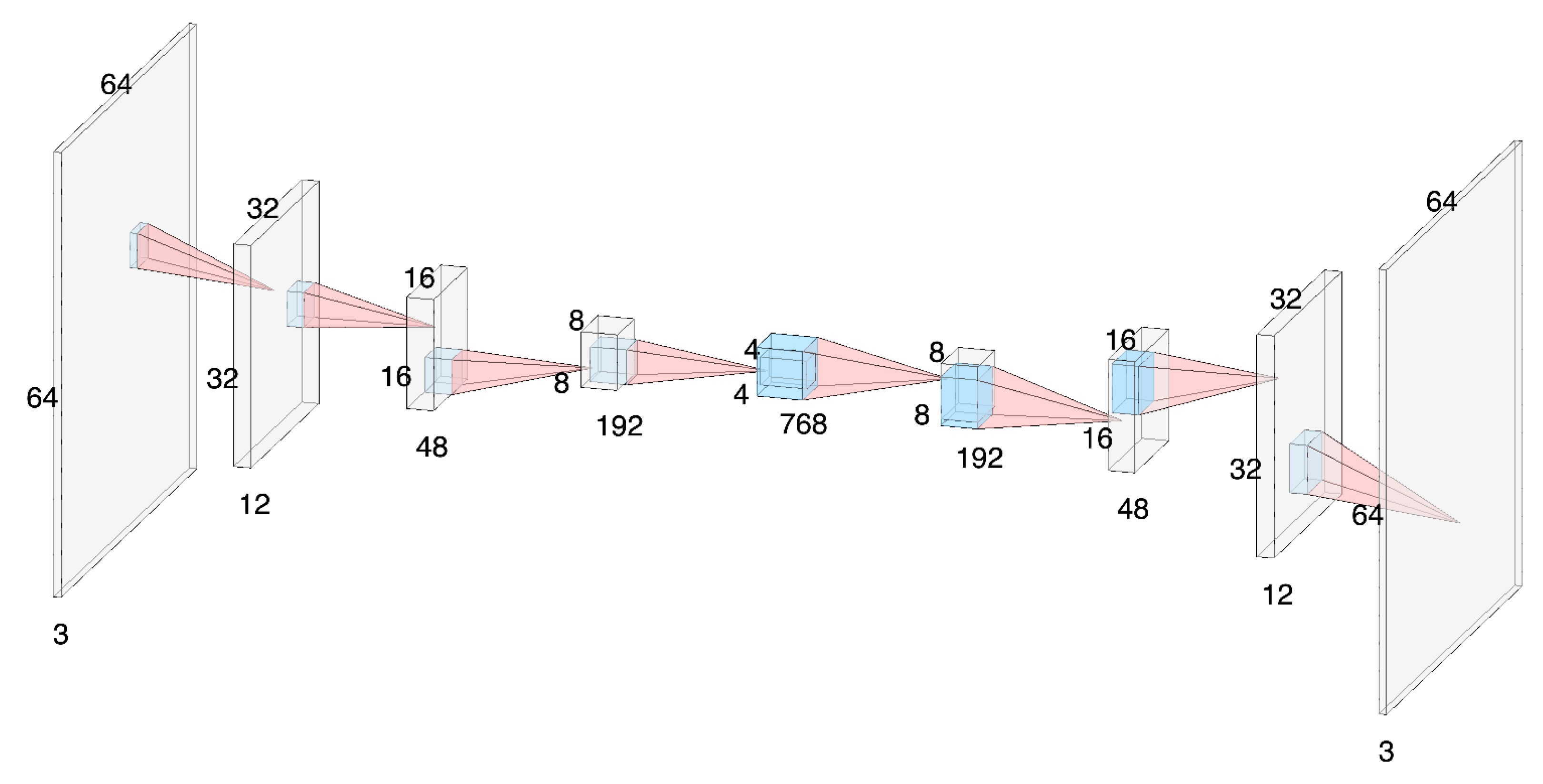
  • The introduction of Principal Component Wavelet Networks (PCWNs) and the demonstration that the resulting architecture is equivalent to a CNN.
  • An inversion algorithm, which allows the trained networks to be used as an autoencoder.
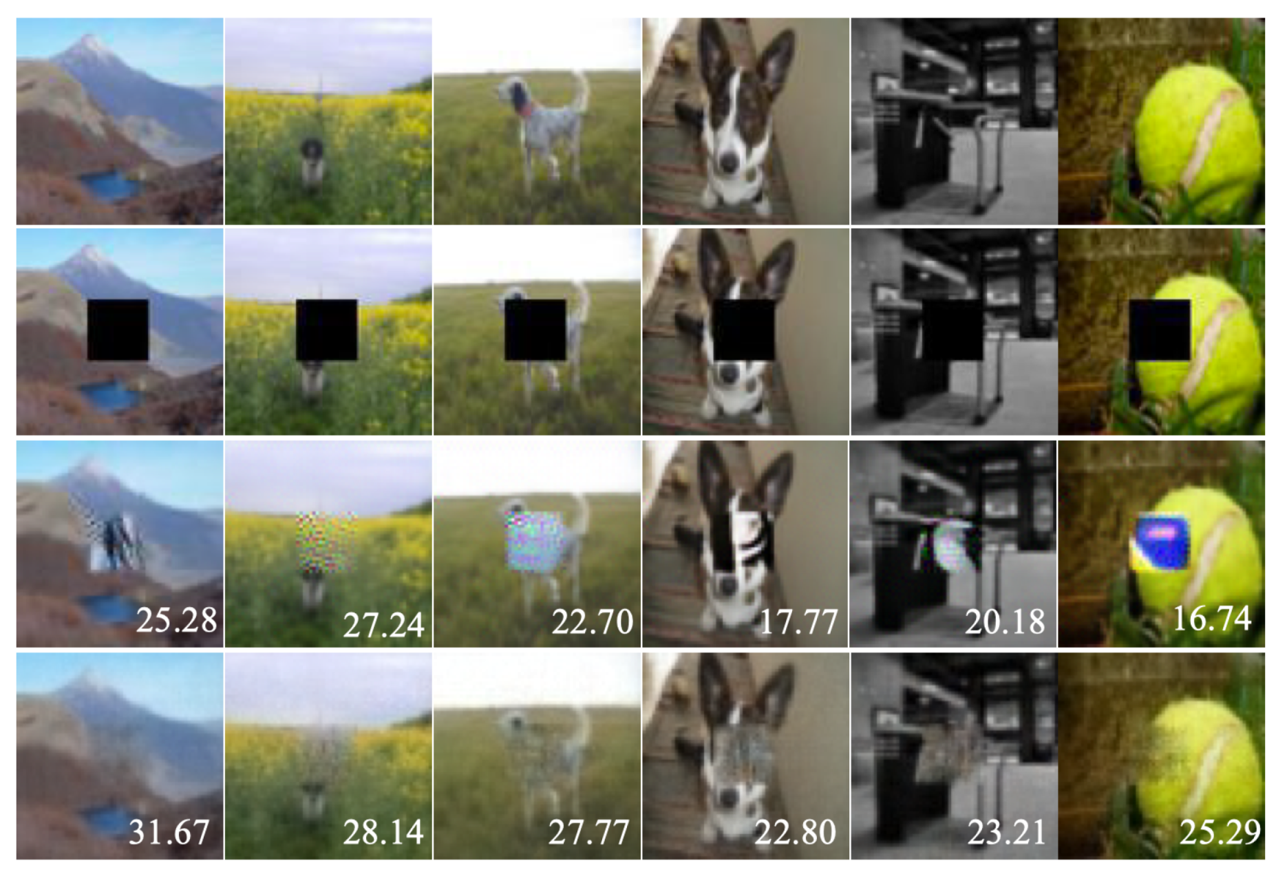
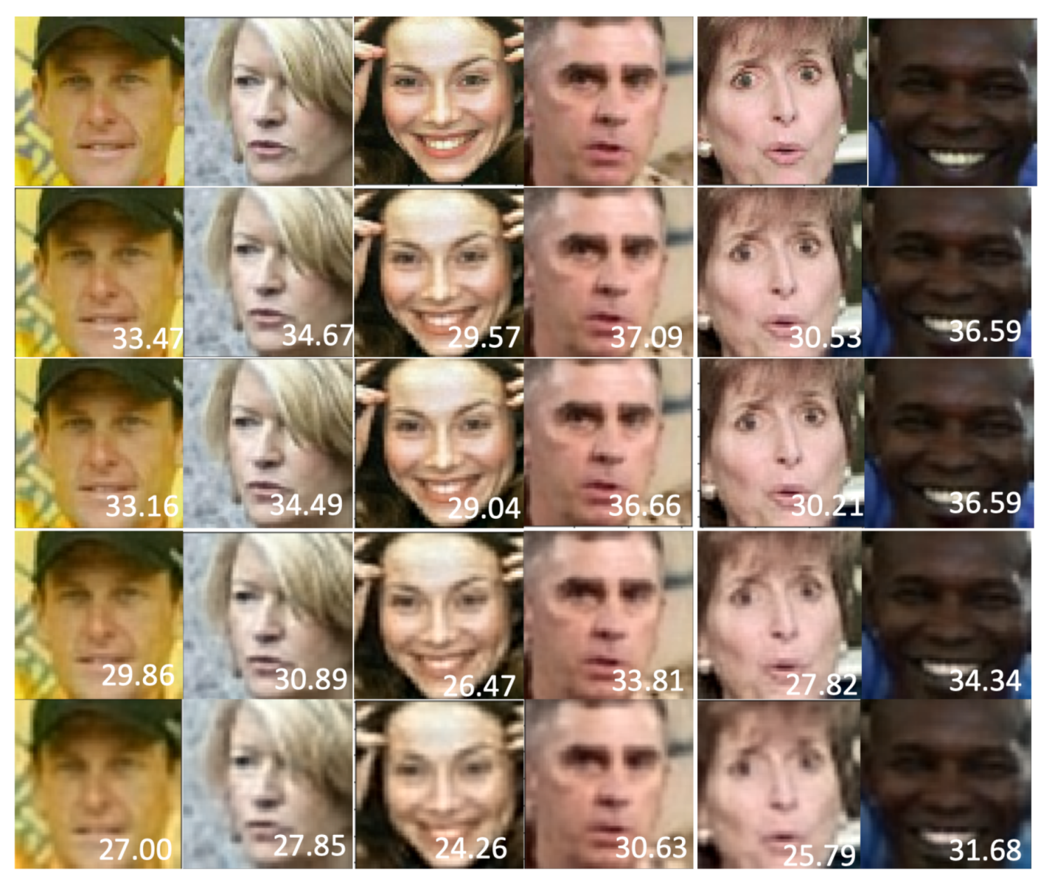
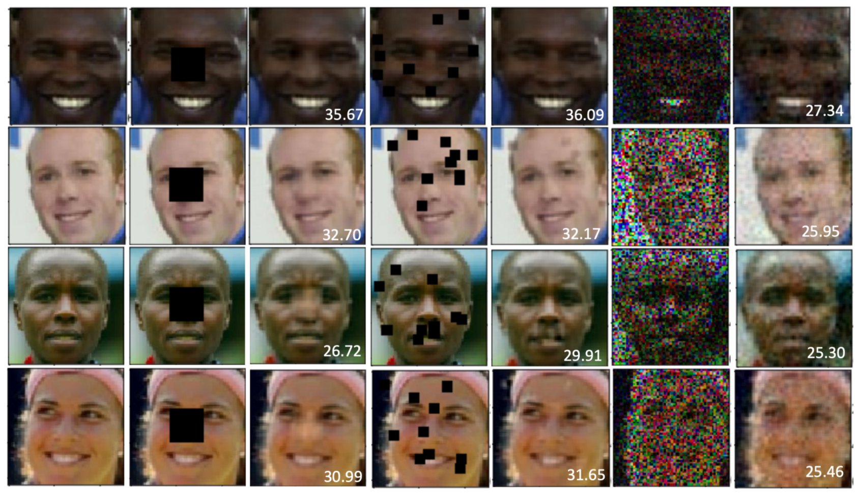
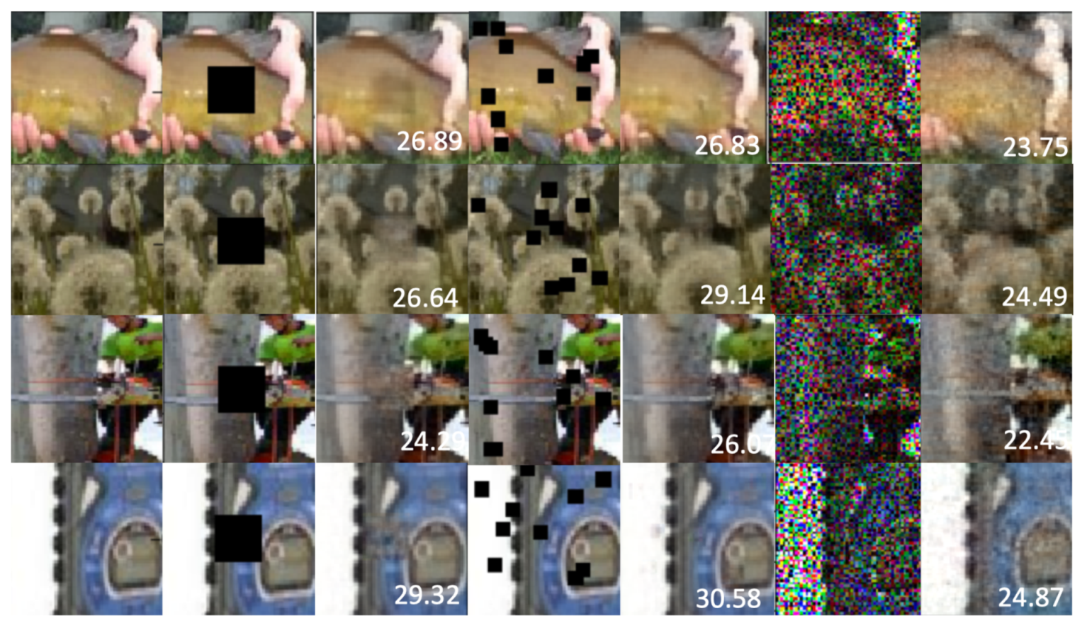
  • An example application to linear inverse problems, where the proposed networks show good potential, outperforming the original OnetNet [12] on 6 out of 9 tasks and showing state-of-the-art performance for a general purpose solution on three tasks (superresolution for face images, and pixelwise inpaint denoising and scattered inpainting on ImageNet).
It is worth noting that, although the structure of the final network is equivalent to a CNN, the training of the proposed network does not involve backpropagation or stochastic optimisation. The simple, forward, deterministic nature of the training algorithm makes the network fast to learn. The use of PCA, which is based on a Gaussian distribution model, leads to an algorithm which is robust against over-fitting, which is a problem with GAN-based methods (as shown in Figure 1). The considerable improvement in ADMM using an L1-norm regulariser based on our decomposition, compared to simpler wavelet-based techniques, indicates an interesting direction of research for novel learning algorithms within the CNN data structure.

4. Method: Decomposition, Training and Reconstruction

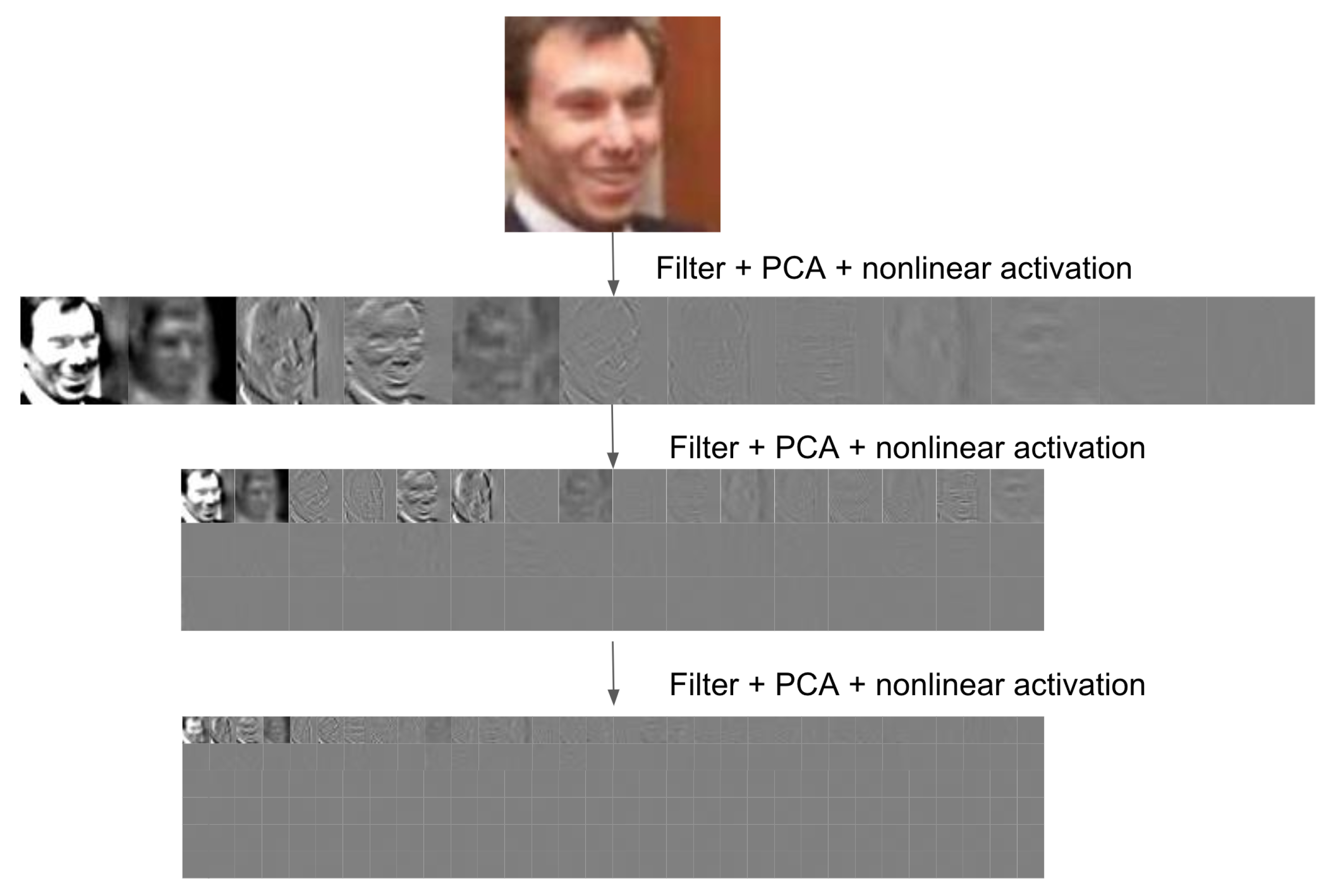
4.1. Decomposition Algorithm

In this section we describe the algorithms for constructing, training and reconstructing a PCWN decomposition. At each level in the decomposition, each channel first undergoes convolution with each filter in the selected filter-bank. For the rest of this paper we use separable filters based on approximations to zeroth, first and second derivatives of a Gaussian. Each is applied along either the x or y direction, leading to nine output channels per input channel. We typically use a stride of two, although other options are possible. This gives rise to:
t l + 1 ( 9 z + 3 j + i ) = G i x G j y s l ( z ) ,
where t l + 1 ( 9 z + 3 j + i ) is the decomposition tensor channel ‘ 9 z + 3 j + i ’ at level ‘ l + 1 ’ of the decomposition prior to PCA processing, s l ( z ) is the decomposition tensor channel z at level l of the decomposition following PCA processing (or the input), G i x and G j y are 1D Gaussian derivatives in direction x and y of order i and j respectively, where i 0 , 1 , 2 and j 0 , 1 , 2 .
After filtering, the channels are projected into the learnt principal component subspace, which forms a weighted sum s l ( z ) of the channels within the subband, t l ( i ) along with a bias term representing subtraction of the mean i.e.,
s l ( z ) = b l ( z ) + i = 0 Z l W l ( z , i ) t l ( i ) .
Here W l ( z , i ) is the ith component of the zth principal component at level l in the decomposition and Z l is the number of channels before projection into the PCA subspace. The bias term b l ( z ) is equivalent to the dot product of the negative of the mean, m l ( i ) , with the principal component:
b l ( z ) = i = 0 Z l W l ( z , i ) m l ( i ) .
Adding this term after taking the dot product is equivalent to subtracting the mean for level l, m l ( i ) , before taking the dot product with W l ( z , i ) .

4.2. Training Algorithm

To learn the PCA decomposition for level l, we iterate through the training set and iteratively decompose using the specified filters and PCA parameters up to level ‘ l 1 ’. We then filter with the specified filters at level l. We form the mean vector across channels as:
m l ( z ) = 1 K X l Y l k = 0 K x = 0 X l y = 0 Y l t l ( x , y , z ) ,
where the sum is over all K training images and all pixels in the X l by Y l subband images. The covariance matrix is similarly formed from the sum of outer-product matrices of these vectors, i.e., if the t l are considered as row vectors:
C l ( z , w ) = 1 K X l Y l 1 k , x , y K , X l , Y l d ( z ) T d ( w )
where d ( q ) = t l ( x , y , q ) m l ( q ) . The above sum can be factored into:
1 K X l Y l 1 k , x , y K , X l , Y l t l ( z ) T t l ( w ) K X l Y l m l ( z ) T m l ( w ) ,
which allows a single pass algorithm per layer of the network. The processing of a single fibre (the vector of values at a specific 2D location) is illustrated in Figure 2.
Eigenanalysis of the covariance matrix C l gives the principal components in the orthonormal matrix W l and their variances in the diagonal matrix Λ l :
C l = W l Λ l W l t .
We order the eigenvectors according to the size of their corresponding eigenvalues, which give the variances along each component. We then drop those with the smallest value according to some criteria, such as: percentage of variance explained; a fixed network architecture; or maximum number of desired channels.
An example of the outputs of each step in the first layer decomposition is shown in Figure 3. The filter bank and 1 × 1 filters are combined into a single 2D convolutional tensor. The result of applying the filter learnt at each level of the decomposition is shown in Figure 4. The output at each level can be combined with an optional non-linear activation function.

4.3. Reconstruction Algorithm

The reconstruction algorithm performs the decomposition steps in reverse. Starting at the lowest level, first the inverse of any non-linear activation function needs to be applied. Then the channels (now principal component weighting images) s l are used to reconstruct approximations t l to the original subband images t l using:
t l ( z ) = m l ( z ) + i = 0 T l W l ( i , z ) s l ( i ) .
where m l ( z ) is the corresponding mean for channel z of level l of the decomposition, T l is the number of principal components that were retained for level l, and W l ( i , z ) is the zth component of the ith principal component at level l in the decomposition.
Next these images are processed in blocks of 9 (for our typical case of 9 construction filters) to reconstruct the matching channel at level ‘ l 1 ’. One way to do this is to construct the filter matrix Φ corresponding to the one dimensional forward filtering (including the stride, border handling etc.) and calculate the least squares inverse (Moore–Penrose pseudo-inverse) Φ :
Φ = ( Φ t Φ ) 1 Φ t .
This is applied along rows and then columns to recreate the channel at the higher level in the decomposition. Another option is to find a set of reconstruction filters with compact support. These form a set of transpose convolution filters that are separable in x and y. An example set of forward and inverse filters is given in Table 1. The entire process for constructing the decompostion and reconstruction networks is outlines in Algorithm 1.
The architecture of the complete network is shown in Figure 5. Examples of reconstructed images with linear and non-linear activation functions (a simple tanh activation function on the decomposition, and atanh on the reconstruction), and varying compression levels (100%, 50% and 25%) for the linear models are shown in Figure 6.
Algorithm 1: Overview of the training algorithm
Symmetry 13 01083 i001

4.4. Discussion of Architecture

The above process allows us to construct CNNs using a very simple yet effective learning process. The learnt network is generic, rather than trained for any specific problem, but is optimal in the sense of minimizing the information loss at each level subject to an orthogonal decomposition. The filters in our method are derived from a local linear model of separable convolution operators and they are not necessarily constrained to be separable. For example the Laplacian can be approximated by the sum of two separable derivative filters, but is not itself separable. As we are forming linear combinations of filtered images via the use of PCA, the resulting filters can include the derivatives steered in different directions (as they span the first and second derivative steerable filter bases), Laplacian and other common filters. In fact, for small filters, such as 3 × 3 commonly used in CNNs, the space of such filters lies in an eight dimensional space, which is spanned by the nine filters used in this work, so the system can learn any 3 × 3 filter. In this work we extend the low-pass filter in order to make the wavelet functions used smoother, which is known to lead to fewer reconstruction artefacts in wavelet processing.
The network can incorporate non-linear elements, such as activation functions between networks, max pooling layers, batch normalisation etc. There is no dependency on learning (as there is for back propagation), but some of these elements make inversion difficult or impossible. For the work described here we focus on linear inverse problems, we need to be able to perform the inverse transform and so leave investigation of these aspects to future work. The structure used in this paper is shown in Figure 5. A simplified table of the layers is shown in Table 2. For the most part the algorithm can be implemented using standard layers (e.g., in Tensorflow Keras). The filters can be applied either separably or pre-calculated into three dimensional ( w i d t h × h e i g h t × c h a n n e l s ) filters for the construction. Symmetric padding is used to handle the borders. For the reconstruction, transpose convolution is used. Due to the use of some anti-symmetric 1D filters, we need to first apply the inverse PCA decomposition to reconstruct the set of original filtered channels. This allows us to use anti-symmetric border padding for the correct handling of the borders of the anti-symmetric filtered channels (performed using regular symmetric padding and multiplication by a mask of mostly 1’s and 1 ’s for the anti-symmetric padding values) (Code available from https://github.com/bptiddeman/PCWN.git or as a Google Colab demo https://colab.research.google.com/drive/1bRji-34Icy8serMzxZ0r-S2FqVOfgw2-?usp=sharing) (accessed on: 17 February 2021).

4.5. Computational Complexity

The computational complexity of the proposed training algorithm is related to the size of the training set, T, the number of levels in the decomposition, L, the number of pixels in each level, N l , and the number of channels retained in each level, C l . For one level of the decomposition, the algorithm requires O ( T N l 2 C l 2 + N l 3 C l 3 ) operations, with the first term resulting from the building of the covariance matrix, and the second term from the Eigenanalysis step of the PCA that is required once per level. The total complexity is found by summing these terms over all levels, O ( l L ( T N l 2 C l 2 + N l 3 C l 3 ) ) . Comparison of this complexity to training a deep learning projection operator is difficult. The deep learning projectors extend the training set by introducing image perturbations, thus effectively increasing T, whereas the PCWN training only requires the original unperturbed images. The PCWN requires a known, fixed number of operations, whereas for stochastic, gradient-based optimisation methods the convergence requires a variable number of iterations to reach a minimum, depending on the characteristics of the problem. For example, OneNet [12] used between 10 K and 80 K iterations on batches of 25 to 32 images. As an indication of the comparative training cost, training onenet on the celeb-a dataset for 6000 iterations on our GPU server using a single GPU (Tesla P100-PCIE-16GB) required over 52 h and was far from converging. The DU-ADMM authors recommend 100,000 iterations in their code, which would take over a month to train on our system. In contrast, we were able to train our system in 4 h for the celeb-a dataset (200 K images), or 15 h for the entire ImageNet training partition (1.2 M images) on the same platform.

4.6. Implementation

The construction algorithm was implemented in Tensorflow 2 using the Keras interface with a number of custom layers. Custom layers were required in particular to handle border symmetry/anti-symmetry correctly for exact reconstruction of the downsampled wavelet filters. The ADMM implementation was adapted from the OneNet implementation [31]. The system was first implemented using Google Colab for development and collaboration, then exported to a Python script for running on our GPU server, a 32-core system with 48 Gb of system RAM, 2 GP100GL graphics cards, each with 16 Gb of VRAM.

5. Example Application: Linear Inverse Problems

Integration with ADMM

ADMM is a standard method for solving linear inverse problems. The minimisation problem (Equation (2)) is split into a number of sub-problems, which are solved iteratively i.e.,
x k + 1 = argmin x ρ 2 | | x z k u k | | 2 + λ ϕ ( x ) ,
z k + 1 = argmin z 1 2 | | y A z | | 2 + ρ 2 | | x k + 1 z u k | | 2 ,
u k + 1 = u k + z k + 1 x k + 1 .
The approach to solving Equation (12), involves the constraint ϕ ( x ) , which is usually taken to be a constraint intended to encourage sparsity of x in some suitable domain, often taken as minimisation of the L 1 norm in that domain i.e.,
x k + 1 = argmin x ρ 2 | | x z k u k | | 2 + λ | x | 1 ,
where primes denote the change to a suitable domain, typically a wavelet domain. The solution to the above minimisation is the proximal function for the L 1 norm, which is found by applying the soft-thresholding operator
x s g n ( x ) m a x ( 0 , | x | ρ λ )
to z k + u k . Hence the update to x is given by soft thresholding in a domain where the signal is expected to be sparse. In this work we use our PCWN as the sparse domain, as described in the preceding section. Equation (13) can be solved directly:
z k + 1 = ( A t A + ρ I ) 1 A t y + ρ ( x k + 1 u k ) .
For problems such as inpainting (pixelwise, scattered, or blockwise), matrix A is a diagonal masking matrix containing 0 for missing data or 1 for included data. For super-resolution Equation (17), A is taken to be a non-overlapping blockwise averaging matrix. For compressive sensing, matrix A is a random matrix of size m × d for images size d ( d = p i x e l s × c h a n n e l s ) where we use m d = 0.1 . In this work we follow [12] and use conjugate gradient solvers for simplicity for all problems. In each iteration, the solver is “warm started” with the solution from the previous iteration and usually converges quickly.
In previous work, such as OneNet [12], the solution was initialised with the least-squares solution to:
x 0 = a r g m i n x | | A x y | | 2 .
In this work, we experiment with an alternative initialisation, using the mean image learnt from the training set as the starting point. The reasoning being that where there is missing data, particularly structured data such as faces, the mean may provide a better approximation than the least-squares solution. This change seems to benefit face images, where the mean is an average, blurry face, but is less helpful with more highly varied datasets, such as ImageNet, where the mean is essentially just a grey image. That said, the solution should converge to the solution independently of the initialisation [32], although better initialisation leads to reaching the optimal value more quickly and so prevents the optimisation stopping before the minimum is reached.

6. Experiments

We evaluated our method against a number of existing general purpose solutions, namely the original OneNet solution [12], the more recent Differential Unrolled ADMM (DU-ADMM) version of OneNet [15] and the general purpose wavelet based method [32].
For face images we trained and tested our method on the Labelled Faces in the Wild (LFW) dataset [33], testing on 300 images, 200 images were reserved for tuning (unused) and the remaining 12,733 images were used for training. The images had the central 50% square (containing the face) cropped and were then downsampled to 64 × 64 . We used 100 iterations for all methods. For blockwise and scattered inpainting, and super-resolution we used λ = 0.1 and ρ = 0.0005 . For pixelwise inpaint denoising with 10% noise we used λ = 0.6 and ρ = 0.003 . For compressive sensing we used λ = 0.1 and ρ = 0.005 .
We compared our results with those of the other methods presented in [15]. For these results the systems were trained on images of 73,678 people and tested on 500 random images from the MS-Celebs-1M dataset. We elected not to use the MS-celeb-1M dataset due to ethical concerns around privacy, which led to the datasets’ website being withdrawn [34]. Although we train and test on different image sets, we believe the results are comparable because:
  • The face images used previously for testing and training were a random subset of the dataset, so even if we used the same dataset they wouldn’t necessarily be the same images.
  • They are both celebrity face images, of the same resolution, scraped off the web, so should be comparable.
  • Deep learning usually benefits from using more data (to avoid overfitting), so arguably we are setting ourselves a harder task or, alternatively, demonstrating that our method is more resistant to overfitting.
We also test our method on images in the ImageNet 2012 dataset downsized to 64 × 64 pixels [35]. We train our model on the full training set and test on 3000 images. We compare with the results published in [12] (for CS) and [15] (for BI, SI, PID, and SR). Although we use the same dataset as those authors, again there is some uncertainty about the specific test images used, so the results should be taken as indicative of the general performance. For blockwise and scattered inpainting, and super-resolution we used λ = 0.1 and ρ = 0.002 . For pixelwise inpaint denoising with 10% noise we used λ = 0.3 and ρ = 0.004 . For compressive sensing we used λ = 0.1 and ρ = 0.004 .

Results

The quantitative results on face images are presented in Table 3 and examples are shown in Figure 7 and Figure 8. We follow previous authors and use the Peak Signal-to-Noise Ratio (PSNR) to assess our results. PSNR is defined as:
P S N R = 20 log 10 M A X R M S
where R M S is the root mean squared error and M A X is the maximum intensity in each channel (usually 255 in images, or 1.0 in intensity normalised images). We report the mean and standard deviation PSNR across the test images to allow meaningful comparison between methods. Our method performs best on the super-resolution task, and better than or equivalent to the original OneNet on Blockwise Inpainting (BI) and Pixelwise Inpaint Denoising (PID) problem, but slightly worse than DU-ADMM. For compressive sensing (CS), quantitative results on face images were not presented previously for face images.
For ImageNet images, we trained our model on the entire training set of 1.2 M images and tested on a separate set of 3000 random images from the validation partition. The quantitative results are presented in Table 4. Example qualitative results for the inpainting problems (blockwise inpaint (BI), scattered inpaint (SI) and pixelwise inpaint denoising (PID)) are shown in Figure 9 and for compressive sensing (CS) and super resolution (SR) are shown in Figure 10.

7. Conclusions and Future Work

In this paper we have proposed Principal Component Wavelet Networks (PCWN) based on a set of specified wavelet functions and combined with PCA to learn 1 × 1 convolution filters for data reduction. We have shown that the resulting decomposition is identical in structure to standard CNNs and permits the option to incorporate nonlinear activation functions. The resulting decomposition is deterministic and based on well studied mathematical models and techniques including wavelet analysis and PCA, making it more amenable to mathematical analysis. We have also shown how to perform (approximate) reconstruction in order to form an easy to learn auto-encoder. We have demonstrated the potential of the proposed technique by using it to solve linear inverse problems. Our experimental results show improved or equivalent performance to the original general purpose OneNet system on many of the example problems. The main advantages of the proposed technique are a fast, simple and deterministic learning algorithm, (as opposed to adversarial learning algorithms that are known to be challenging to train) and, with PCA being based on a Gaussian model, is not prone to overfitting as exhibited in the OneNet method, particularly in Blockwise Inpainting, as shown in Figure 1. Disadvantages include slower convergence of the ADMM method and lower quality results on some of the problems presented. Future work will include evaluating the proposed decomposition technique for other problems, and improving the linear inverse solving system. A significant issue with the current system is selecting suitable parameters to obtain good results on a particular problem/image set combination. We will investigate methods for learning good parameters from the training data. As with CNNs, there are an infinite variety of architectures, including layers, strides, activation functions etc. which can be varied for different problems. Here we only use a simple pyramidal architecture and linear activation functions. We plan to investigate alternatives for both the linear inverse problems and other common vision and image processing problems in future work. As an encoder-decoder network, it also has potential for application to other common problems such as colorization e.g., [36], classification e.g., for remote sensing [37]. As the model is based on a well studied statistical model, it may be amenable to other techniques such as detecting/avoiding outliers [38] or extreme values [39] which may make the systems more robust.

Author Contributions

Software: B.T. and M.G.; methodology: B.T.; manuscript preparation: B.T. and M.G.; experiments: B.T. and M.G. proof reading: B.T. and M.G. All authors have read and agreed to the published version of the manuscript.

Funding

M.G. is funded by an Aberystwyth University PhD Scholarship.

Data Availability Statement

The data used is in the public domain. The code has been made available from https://github.com/bptiddeman/PCWN.git or as a Google Colab demo https://colab.research.google.com/drive/1bRji-34Icy8serMzxZ0r-S2FqVOfgw2-?usp=sharing (accessed on 17 February 2021).

Conflicts of Interest

The authors declare no conflict of interest.

References

  1. Donoho, D.L. De-noising by soft-thresholding. IEEE Trans. Inf. Theory 1995, 41, 613–627. [Google Scholar] [CrossRef] [Green Version]
  2. Portilla, J.; Strela, V.; Wainwright, M.J.; Simoncelli, E.P. Image denoising using scale mixtures of Gaussians in the wavelet domain. IEEE Trans. Image Process. 2003, 12, 1338–1351. [Google Scholar] [CrossRef] [Green Version]
  3. Mairal, J.; Sapiro, G.; Elad, M. Learning multiscale sparse representations for image and video restoration. Multiscale Model. Simul. 2008, 7, 214–241. [Google Scholar] [CrossRef] [Green Version]
  4. Chan, T.F.; Shen, J.; Zhou, H.M. Total variation wavelet inpainting. J. Math. Imaging Vis. 2006, 25, 107–125. [Google Scholar] [CrossRef]
  5. Dong, W.; Zhang, L.; Shi, G.; Wu, X. Image deblurring and super-resolution by adaptive sparse domain selection and adaptive regularization. IEEE Trans. Image Process. 2011, 20, 1838–1857. [Google Scholar] [CrossRef] [Green Version]
  6. Pathak, D.; Krahenbuhl, P.; Donahue, J.; Darrell, T.; Efros, A.A. Context encoders: Feature learning by inpainting. In Proceedings of the IEEE Conference on Computer Vision and Pattern Recognition, Las Vegas, NV, USA, 27–30 June 2016; pp. 2536–2544. [Google Scholar]
  7. Mousavi, A.; Baraniuk, R.G. Learning to invert: Signal recovery via deep convolutional networks. In Proceedings of the 2017 IEEE international conference on acoustics, speech and signal processing (ICASSP), New Orleans, LA, USA, 5–9 March 2017; pp. 2272–2276. [Google Scholar]
  8. Kulkarni, K.; Lohit, S.; Turaga, P.; Kerviche, R.; Ashok, A. Reconnet: Non-iterative reconstruction of images from compressively sensed measurements. In Proceedings of the IEEE Conference on Computer Vision and Pattern Recognition, Las Vegas, NV, USA, 27–30 June 2016; pp. 449–458. [Google Scholar]
  9. Ledig, C.; Theis, L.; Huszár, F.; Caballero, J.; Cunningham, A.; Acosta, A.; Aitken, A.; Tejani, A.; Totz, J.; Wang, Z.; et al. Photo-realistic single image super-resolution using a generative adversarial network. In Proceedings of the IEEE Conference on Computer Vision and Pattern Recognition, Honolulu, HI, USA, 21–26 July 2017; pp. 4681–4690. [Google Scholar]
  10. Dong, C.; Loy, C.C.; He, K.; Tang, X. Learning a deep convolutional network for image super-resolution. In Proceedings of the European Conference on Computer Vision, Zurich, Switzerland, 6–12 September 2014; Springer: Berlin/Heidelberg, Germany, 2014; pp. 184–199. [Google Scholar]
  11. Xu, L.; Ren, J.S.; Liu, C.; Jia, J. Deep convolutional neural network for image deconvolution. In Proceedings of the Advances in Neural Information Processing Systems, Montreal, QC, Canada, 8–13 December 2014; pp. 1790–1798. [Google Scholar]
  12. Rick Chang, J.; Li, C.L.; Poczos, B.; Vijaya Kumar, B.; Sankaranarayanan, A.C. One Network to Solve Them All–Solving Linear Inverse Problems Using Deep Projection Models. In Proceedings of the IEEE International Conference on Computer Vision, Venice, Italy, 22–29 October 2017; pp. 5888–5897. [Google Scholar]
  13. Lucic, M.; Kurach, K.; Michalski, M.; Bousquet, O.; Gelly, S. Are GANs Created Equal? A Large-Scale Study. In Proceedings of the 32nd International Conference on Neural Information Processing Systems (NIPS’18), Montreal, QC, Canada, 3–8 December 2018; Curran Associates Inc.: Red Hook, NY, USA, 2018; pp. 698–707. [Google Scholar]
  14. Arjovsky, M.; Bottou, L. Towards Principled Methods for Training Generative Adversarial Networks. In Proceedings of the 5th International Conference on Learning Representations (ICLR 2017), Toulon, France, 24–26 April 2017. [Google Scholar]
  15. Milacski, Z.A.; Póczos, B.; Lorincz, A. Differentiable Unrolled Alternating Direction Method of Multipliers for OneNet. In Proceedings of the British Machine Vision Conference, Cardiff, UK, 9–12 September 2019. [Google Scholar]
  16. Raj, A.; Li, Y.; Bresler, Y. GAN-Based Projector for Faster Recovery With Convergence Guarantees in Linear Inverse Problems. In Proceedings of the 2019 IEEE/CVF International Conference on Computer Vision (ICCV), Seoul, Korea, 27 October–2 November 2019; pp. 5601–5610. [Google Scholar]
  17. Mallat, S. A Wavelet Tour of Signal Processing, 3rd ed.; Academic Press: Cambridge, MA, USA, 2008; pp. 1–832. [Google Scholar]
  18. Freeman, W.T.; Adelson, E.H. The design and use of steerable filters. IEEE Trans. Pattern Anal. Mach. Intell. 1991, 13, 891–906. [Google Scholar] [CrossRef]
  19. Kingsbury, N. Complex wavelets for shift invariant analysis and filtering of signals. J. Appl. Comput. Harmon. Anal. 2001, 10, 234–253. [Google Scholar] [CrossRef] [Green Version]
  20. Selesnick, I.W.; Baraniuk, R.G.; Kingsbury, N.C. The dual-tree complex wavelet transform. IEEE Signal Process. Mag. 2005, 22, 123–151. [Google Scholar] [CrossRef] [Green Version]
  21. Selesnick, I.W. The double-density dual-tree DWT. IEEE Trans. Signal Process. 2004, 52, 1304–1314. [Google Scholar] [CrossRef]
  22. Kingma, D.P.; Dhariwal, P. Glow: Generative flow with invertible 1x1 convolutions. In Proceedings of the Advances in Neural Information Processing Systems, Montreal, QC, Canada, 3–8 December 2018; pp. 10215–10224. [Google Scholar]
  23. Bruna, J.; Mallat, S. Invariant Scattering Convolution Networks. IEEE Trans. Pattern Anal. Mach. Intell. 2013, 35, 1872–1886. [Google Scholar] [CrossRef] [Green Version]
  24. Oyallon, E.; Zagoruyko, S.; Huang, G.; Komodakis, N.; Lacoste-Julien, S.; Blaschko, M.; Belilovsky, E. Scattering networks for hybrid representation learning. IEEE Trans. Pattern Anal. Mach. Intell. 2018, 41, 2208–2221. [Google Scholar] [CrossRef] [PubMed] [Green Version]
  25. Angles, T.; Mallat, S. Generative networks as inverse problems with scattering transforms. arXiv 2018, arXiv:1805.06621. [Google Scholar]
  26. Gupta, M.R.; Jacobson, N.P. Wavelet Principal Component Analysis and its Application to Hyperspectral Images. In Proceedings of the 2006 International Conference on Image Processing, Las Vegas, NV, USA, 26–29 June 2006; pp. 1585–1588. [Google Scholar] [CrossRef]
  27. Feng, G.C.; Yuen, P.C.; Dai, D.Q. Human face recognition using PCA on wavelet subband. J. Electron. Imaging 2000, 9, 226–233. [Google Scholar]
  28. Naik, G.R.; Pendharkar, G.; Nguyen, H.T. Wavelet PCA for automatic identification of walking with and without an exoskeleton on a treadmill using pressure and accelerometer sensors. In Proceedings of the 2016 38th Annual International Conference of the IEEE Engineering in Medicine and Biology Society (EMBC), Orlando, FL, USA, 16–20 August 2016; pp. 1999–2002. [Google Scholar] [CrossRef] [Green Version]
  29. Chan, T.H.; Jia, K.; Gao, S.; Lu, J.; Zeng, Z.; Ma, Y. PCANet: A simple deep learning baseline for image classification? IEEE Trans. Image Process. 2015, 24, 5017–5032. [Google Scholar] [CrossRef] [Green Version]
  30. Kong, J.; Chen, M.; Jiang, M.; Sun, J.; Hou, J. Face recognition based on CSGF (2D) 2 PCANet. IEEE Access 2018, 6, 45153–45165. [Google Scholar] [CrossRef]
  31. Rick Chang, J.; Li, C.L.; Poczos, B.; Vijaya Kumar, B.; Sankaranarayanan, A.C. OneNet Tensorflow Implementation. Available online: https://github.com/rick-chang/OneNet/tree/master/admm (accessed on 17 February 2021).
  32. Wang, Y.; Yin, W.; Zeng, J. Global convergence of ADMM in nonconvex nonsmooth optimization. J. Sci. Comput. 2019, 78, 29–63. [Google Scholar] [CrossRef] [Green Version]
  33. Huang, G.B.; Ramesh, M.; Berg, T.; Learned-Miller, E. Labeled Faces in the Wild: A Database for Studying Face Recognition in Unconstrained Environments; Technical Report 07-49; University of Massachusetts: Amherst, MA, USA, 2007. [Google Scholar]
  34. Harvey, A.; LaPlace, J. MegaPixels: Origins, Ethics, and Privacy Implications of Publicly Available Face Recognition Image Datasets. 2019. Available online: https://megapixels.cc (accessed on 17 February 2021).
  35. Russakovsky, O.; Deng, J.; Su, H.; Krause, J.; Satheesh, S.; Ma, S.; Huang, Z.; Karpathy, A.; Khosla, A.; Bernstein, M.; et al. ImageNet Large Scale Visual Recognition Challenge. Int. J. Comput. Vis. 2015, 115, 211–252. [Google Scholar] [CrossRef] [Green Version]
  36. Joshi, M.R.; Nkenyereye, L.; Joshi, G.P.; Islam, S.M.R.; Abdullah-Al-Wadud, M.; Shrestha, S. Auto-Colorization of Historical Images Using Deep Convolutional Neural Networks. Mathematics 2020, 8, 2258. [Google Scholar] [CrossRef]
  37. Rajendran, G.B.; Kumarasamy, U.M.; Zarro, C.; Divakarachari, P.B.; Ullo, S.L. Land-Use and Land-Cover Classification Using a Human Group-Based Particle Swarm Optimization Algorithm with an LSTM Classifier on Hybrid Pre-Processing Remote-Sensing Images. Remote Sens. 2020, 12, 4135. [Google Scholar] [CrossRef]
  38. Jäntschi, L. A Test Detecting the Outliers for Continuous Distributions Based on the Cumulative Distribution Function of the Data Being Tested. Symmetry 2019, 11, 835. [Google Scholar] [CrossRef] [Green Version]
  39. Jäntschi, L. Detecting Extreme Values with Order Statistics in Samples from Continuous Distributions. Mathematics 2020, 8, 216. [Google Scholar] [CrossRef] [Green Version]
Figure 1. Examples of Blockwise Inpainting, where GAN based methods can be prone to overfitting but our network is not. Rows from top to bottom: original images; the masked input images; the outputs of OneNet [12] showing evidence of overfitting; the results of our network. The figures show the PSNR of the output images. We have reproduced the examples selected by the authors of [12] using their code [31]. The OneNet examples in [15] show similar problems for blockwise inpainting.
Symmetry 13 01083 g001
Figure 2. Illustration of the accumulation of the sum of ‘fibres’ and their outer products used to compute the mean and covariance matrix in a single pass through all images per output layer.
Symmetry 13 01083 g002
Figure 3. An example of the first stage of the decomposition. First, each channel is filtered with each of the specified filter banks. Second, a set of 1 × 1 × c h a n n e l s filters (learnt from PCA) are applied to reduce the number of channels. It is clear that most of the power is concentrated in a small set of channels. After the application of PCA the number of channels is reduced and the remaining ones are generally those with more of the signal energy.
Symmetry 13 01083 g003
Figure 4. An example of multiple stages of the decomposition. The decomposed image tensor is filtered with the convolutional filter formed from the combined filter bank and PCA filters. An optional non-linear activation function can be applied to the output at each stage. Although many of the channels may provide a small amount of the signal energy, the redundancy is significantly reduced with the application of PCA.
Symmetry 13 01083 g004
Figure 5. Architecture of the simple example network used in this paper.
Symmetry 13 01083 g005
Figure 6. Example reconstructions with different variations on the architecture. The top row shows the original image. The second row shows the reconstruction using a decomposition that retains 100% of the information (the decomposition is the same size as the input images) and a linear activation function. The third row shows the results of retaining 100% of the data and using a non-linear activation function (tanh on the decomposition and atanh on the reconstruction). The fourth and fifth rows use a linear activation function and retain 50% and 25% respectively. The PSNR is shown for each reconstructed image.
Symmetry 13 01083 g006
Figure 7. Example results from our network on the blockwise (BI), scattered (SI) and pixelwise denoise (PID) inpainting problems after 100 iterations. Columns from left to right: original image, BI input, BI output, SI input, SI output, PID input and PID output. The figures show the Peak Signal to Noise Ratio (PSNR) of the output image.
Symmetry 13 01083 g007
Figure 8. Example results from our network on the compressive sensing (CS) and super resolution (SR) problems on Labelled Faces in the Wild images after 100 iterations. Columns from left to right: original image, CS output, SR input, SR output. The figures show the PSNR of the output image.
Symmetry 13 01083 g008
Figure 9. Example ImageNet results from our network on the blockwise (BI), scattered (SI) and pixelwise denoise (PID) inpainting problems after 100 iterations. Columns from left to right: original image, BI input, BI output, SI input, SI output, PID input and PID output. The figures show the PSNR of the output image.
Symmetry 13 01083 g009
Figure 10. Example ImageNet results from our network on the compressive sensing CS problem (300 iterations) and super resolution SR problem (100 iterations). Columns from left to right: original image, CS output, SR input, SR output. The figures show the PSNR of the output image.
Symmetry 13 01083 g010
Table 1. Table showing the coefficients of the construction ( G ) and reconstruction ( H ) filters used in this paper.
FilterFilter Coefficients
G 0 × 16 14641
G 1 × 4 0−12−10
G 2 × 2 010−10
H 0 × 16 0018148100
H 1 × 128 −1−8−20−56170−56−20−8−1
H 2 × 256 18301360−136−30−8−1
Table 2. This table shows the structure of our convolutional network.
Input SizeType/StrideFilter Shape
64 × 64 × 3 Subtract mean 64 × 64 × 3
64 × 64 × 3 Conv2D/s2 5 × 5 × 3 × 12
32 × 32 × 12 Conv2D/s2 5 × 5 × 12 × 48
16 × 16 × 48 Conv2D/s2 5 × 5 × 48 × 192
8 × 8 × 192 Conv2D/s2 5 × 5 × 192 × 768
4 × 4 × 768 Decomposition-
4 × 4 × 768 Activation-
4 × 4 × 768 Conv2DTranspose/s2 9 × 9 × 768 × 192
8 × 8 × 192 Conv2DTranspose/s2 9 × 9 × 192 × 48
16 × 16 × 48 Conv2DTranspose/s2 9 × 9 × 48 × 12
32 × 32 × 12 Conv2DTranspose/s2 9 × 9 × 12 × 3
64 × 64 × 3 Add mean 64 × 64 × 3
64 × 64 × 3 Reconstruction-
Table 3. The results of our method compared to other methods on face images, including GAN based approaches (DU-ADMM and OneNet) for Blockwise Inpainting (BI), Super Resolution (SR), Pixelwise Inpainting Denoising (PID), Compressive Sensing (CS) and Scattered Inpainting (SI). Figures show the mean and standard deviation Peak Signal to Noise Ration (PSNR) across the test set.
MethodBISRPIDCSSI
DU-ADMM 28.59 ± 2.3 28.19 ± 3.1 26.87 ± 1.2 - 30.66 ± 1.9
OneNet 24.4 ± 2.4 27.15 ± 1.9 25.39 ± 1.6 - 25.23 ± 2.4
Wavelet 17.70 ± 1.9 28.66 ± 1.7 20.81 ± 1.0 - 28.60 ± 2.4
Ours 27.7 ± 2.3 29.98 ± 2.2 25.32 ± 0.9 23.6 ± 1.9 29.60 ± 2.3
Table 4. The results of our method compared to other methods on ImageNet, including GAN based approaches (DU-ADMM and OneNet) for Blockwise Inpainting (BI), Super Resolution (SR), Pixelwise Inpainting Denoising (PID), Compressive Sensing (CS) and Scattered Inpainting (SI). Figures show the mean and standard deviation Peak Signal to Noise Ration (PSNR) across the test set.
MethodBISRPIDCSSI
DU-ADMM 26.59 ± 3.0 26.38 ± 2.5 24.91 ± 1.8 - 27.92 ± 2.5
OneNet 22.25 ± 2.9 26.11 ± 3.0 25.44 ± 1.8 27.34 ± 5.2 22.85 ± 2.6
Wavelet 19.33 ± 2.9 26.70 ± 2.4 20.18 ± 1.5 13.79 ± 3.7 27.65 ± 2.8
Ours 26.09 ± 2.3 23.1 ± 2.9 27.87 ± 2.8 25.73 ± 2.0 28.04 ± 2.3
Publisher’s Note: MDPI stays neutral with regard to jurisdictional claims in published maps and institutional affiliations.

