Abstract
In this review, we give a basic introduction to the -deformed relativistic phase space and free quantum fields. After a review of the -Poincaré algebra, we illustrate the construction of the -deformed phase space of a classical relativistic particle using the tools of Lie bi-algebras and Poisson–Lie groups. We then discuss how to construct a free scalar field theory on the non-commutative -Minkowski space associated to the -Poincaré and illustrate how the group valued nature of momenta affects the field propagation.
1. Introduction
Quantum group deformations of relativistic spacetime symmetries became a popular topic in the quantum gravity research community in the early 2000s mainly thanks to the development of the ideas of doubly special relativity (DSR), proposed by Amelino-Camelia in two papers [1,2]. These papers pose the question of whether it is possible to reconcile Lorentz invariance with the presence of a minimal length that all inertial observers agree on. Indeed, as it turns out, the existence of a minimal length is a common feature of most, if not all, quantum gravity models (see [3] for review). However, if Lorentz symmetry is to hold, how is it possible that this length scale does not depend on the observer measuring it? As an example, let us consider one of the major results of loop quantum gravity: the discreteness of the spectrum of area and volume operators, with their spectra bounded from below, by, roughly, and , where ℓ is the Planck length. Both areas and volumes, however, are not invariant under Lorentz transformations, so the question arises of which observer should be singled out to measures the minimal length. If such length is indeed minimal, does it mean that its existence implies a violation of Lorentz invariance, under the form of a privileged coordinate system, in which such length takes its minimal value? However, if this is the case, how is this possible in a theory which is built on the very notion of local Lorentz invariance?
The answer that DSR provides to this conundrum is by making the Planck length play the same role as the speed of light plays in special relativity, namely that of an observer-independent scale. The transition from special relativity to DSR is analogous to the route that Einstein chose to take in his way from Galilean relativity to special relativity. As is well known, the presence of an observer-independent scale of speed is not compatible with Galilean relativity. In the transition from non-relativistic to relativistic physics, Einstein did not want to abandon the principle of relativity (of inertial observers); instead, he modified the transformation rules, replacing Galilean transformations by Lorentz ones, in which the speed of light is an observer-independent scale, guaranteed to be the same for all inertial observers. Similarly, in DSR, one adds yet another scale, of length or mass, which is kept observer independent by an appropriate modification of Lorentz transformations, making them nonlinear in such a way that the scale of length/mass is kept invariant. We therefore have to do with a series of transitions from a theory with no observer-independent scales (Galilean relativity), to one with a single scale (special relativity), and finally to the one with two (doubly special relativity). This explains the adjective ‘doubly’ in DSR.
Although DSR was formulated as general scheme, it was clear from the beginning that there is a particular realization of this idea, known under the name of -deformation (another realization that attracted a lot of attention was put forward by Magueijo and Smolin [4,5]) developed in the 1990s in a series of papers [6,7,8,9,10]. Soon after the DSR proposal was put forward, it was noted [11,12] that the deformation of the Poincaré algebra, known under the name of the -Poincaré algebra, can properly describe the symmetries of DSR theories. The -Poincaré algebra is a generalization of the Poincaré algebra admitting another invariant, observer-independent scale, the scale of mass , identified with the Planck mass, as its built-in deformation parameter. When this parameter goes to infinity , -Poincaré becomes the standard Poincaré algebra of special relativity.
The -Poincaré algebra was originally derived as contraction limit of the quantum anti-de Sitter algebra [6,7,9]. It turned out that the deformation parameter of the resulting Hopf algebra, denoted by , is by construction dimensionful, with dimension of mass. Since Poincaré symmetry is a symmetry of flat spacetime, it was natural to speculate, just for dimensional reasons, that -Poincare symmetry must have something to do with quantum gravity, and therefore it is to be expected that the parameter should be of order of the quantum gravity energy scale, the Planck mass, GeV.
The Poincaré algebra can be seen as describing the symmetries of a relativistic system with flat momentum space. From such flat momentum space, one can construct the dual object, the flat Minkowski spacetime on which there exists a natural action of the Poincaré group. In the deformed case, the situation is analogous, but with important and interesting differences. First, the spacetime dual to the momentum space associated with the deformed -Poincaré algebras is non-commutative, with the non-commutativity scale ℓ equal to the inverse of and thus on the order of the Planck length, m [8,10]. Second, the geometry of momentum space becomes non-trivial: the -momentum space has a form of the manifold of the group , being a submanifold of de Sitter space with constant curvature proportional to [13,14,15]. The momentum space with non-trivial geometry was first proposed and analyzed by Max Born [16], and it was revived in the context of noncommutative geometry and Hopf algebras by Majid [17].
As mentioned above, it was very clear from the early days of -deformation that it has to by closely related with quantum gravity. Surprisingly, a direct link has been hard to establish, despite numerous attempts (see, e.g., [18,19,20]). Only a few years ago, a proof of the emergence of -deformation from quantum gravity in the simplified context of Euclidean quantum gravity appeared [21] (see also [22]). The starting observation of this paper is that the algebra of constraints of classical gravity contains, in flat space, the Poincaré algebra as its subalgebra. One can then pose a question of what is the quantum gravity counterpart of the Poincaré algebra, by computing the algebra of quantum commutators of the quantum constraint operators and analyzing their subalgebra corresponding to the classical Poincaré algebra. It turns out that this quantum Poincaré algebra, being an algebra of symmetries of quantum flat spacetime, is, in fact, -Poincaré. It should be mentioned that there is another deformation of spacetime symmetries, the Drinfeld double deformation, obtained with the help of path integral [23,24] and Hamiltonian analysis [25,26,27,28]. Unfortunately, very little is known about the possible extension of these results to 3 + 1 physical dimensions.
In this review, we do not attempt to give a comprehensive overview of the theory of -deformations, as we do that in the upcoming monograph [29]. Instead, we concentrate on some aspects that we found most relevant and that will allow us to touch upon a variety of topics in this vast field. The plan of the paper is as follows. In the next section, we give a pedagogical introduction to the -Poincaré algebra and discuss in some detail its Hopf algebraic structure and geometric aspects. Section 3 is devoted to the description of -deformed phase space using first algebraic tools and then a model of -deformed relativistic particle action. Finally, Section 4 describes some elements of the construction of a -deformed field theory and deformed field propagation. We conclude this review with a brief outlook of the open challenges in the field.
2. The -Poincaré Hopf Algebra
The symmetries of ordinary relativistic kinematics are described by the group of isometries of Minkowski spacetime: the Poincaré group. This group is given by the semidirect product of the abelian group of four-dimensional translations and the non-compact group of Lorentz transformations
A Poincaré transformation by an element on a four vector in Minkowski spacetime is given by
or in terms of the action of a 5 × 5 matrix on a five-vector
Being a semidirect product group, the group multiplication law is given by
with inverse
The Lie algebra of can be easily obtained [30] by writing a Poincaré transformation as a unitary operator and considering its infinitesimal version in terms of the generators of the Lorentz group and of spacetime translations :
with and infinitesimal parameters. To derive the commutators of the Poincaré–Lie algebra, one can write the action by conjugation of a generic element of on the infinitesimal element (6)
and equate it to
giving the following expressions for the adjoint action of the group on its generators:
Specializing (9) and (10) to the case of infinitesimal transformations, one obtains from (9) that
and
while, from (10), one gets
The Lie brackets (11)–(13) define the Poincaré–Lie algebra , which can be written explicitly in terms of the generators of rotations and boosts
(no summation over repeated indices in the first definition) as
As mentioned in the Introduction, the characterizing feature of deformed symmetries is the Lie group manifold structure of four-momentum space with curvature determined by the deformation parameter. Let us be more specific. The configuration space of a spinless relativistic particle in Minkowski spacetime can be identified with the abelian group of translations . The four-momentum space is given by the cotangent space at any of the configuration space , where stands for the dual, as a vector space, to [31]. The phase space of the particle is thus described by the cotangent bundle
Let us denote the Lie algebras associated to each component of as and for and , respectively, and the coordinates for as and for , with . For Lie algebra , we denote the basis elements as , whereas, for , we use . The trivial Lie brackets on the Lie algebras and are
The basic feature of -deformation is that the four-momentum space is no longer a vector space but it becomes a non-abelian Lie group. Such group is the four-dimensional abelian nilpotent group which, as a manifold, is half of de Sitter space whose cosmological constant determines the deformation parameter . We should remark that, in order for this group manifold to be a good candidate for a relativistic four-momentum space, it should admit an action of the Lorentz group on its elements. This is ensured by the fact that both and are subgroups of the de Sitter group . This feature is evident from the factorization of the group known as Iwasawa decomposition [32]. Such decomposition can be described starting from the vector space of the Lie algebra written as a direct sum of vector spaces of its subalgebras
where algebra is the algebra, is the one dimensional algebra described by the matrix
and is the algebra spanned by the elements
where are unit vectors in ith direction (, etc.), and T denotes transposition. Every element of the algebra is a negative root of the element H, i.e.,
We can rescale the elements of the Lie algebras and using the dimensionful deformation parameter in order to have new generators with dimensions of length and which we can see as coordinates on a non-commutative spacetime
known as the -Minkowski spacetime. This commutator replaces the trivial one (21) characterizing an ordinary relativistic particle. From the decomposition (22), it follows that every element of the group can be written as
where , the element belongs to group generated by H
and the element belongs to group generated by algebra
and =diag(−1, 1, 1, 1, −1). The group can be characterized by the factorization
in which its elements can be seen as plane waves on -Minkowski spacetime with the time component ordered to the right
Notice that, while the -Minkowski coordinates are the generators of the non-abelian Lie algebra characterized by the commutator (26), the Lie algebra of translation generators remains abelian
as for an ordinary relativistic particle (21). The elements appearing in (30) are coordinate functions on the group and are known as bicrossporduct coordinates. The quotient group structure of which can be derived from the Iwasawa decomposition of its Lie algebra (22), allows us to obtain another system of coordinates widely used in the literature. Indeed, the quotient of Lie groups is de Sitter space, a symmetric space with a transitive action of [32]. Acting with the an element of the group written as product of matrices on the point
we obtain the coordinates
These coordinates satisfy the constraint
defining de Sitter space as a submanifold of a five-dimensional Minkowski space. It should be noted that the coordinates , describe only half of de Sitter space and therefore the group is not the whole group . However, if we consider the combinations
we cover the whole group which can thus be written in the form
We now describe a crucial feature of -deformation. Let us start by noticing that the coordinates are just specific functions on the part of
Looking at the group element (30) written as a plane wave and using the Baker–Campbell–Hausdorff formula
which in the particular case of takes the form
it is easy to see that
Using this property for the product of two group elements, we get
In other words, the four-momentum of a plane wave obtained by multiplying two plane-waves labeled by four-momenta and is given by the non-abelian sum
Such non-abelian composition law for momenta is the distincitve feature of Hopf algebra deformations of relativistic symmetries. Indeed, if one thinks of plane waves as irreducible representations of the undeformed algebra of translation generators (31), taking the kets and as representatives of the two plane waves above, the non-abelian composition law above can be interpreted as a non-trivial action of the translation generators on the tensor product state
To see this, let us remember that the ordinary composition law for four-momenta can be derived from the fact that the kets and are eigenstates of the translation generators and the fact that the latter act following the Leibniz rule on tensor product states
so that
It turns out that, roughly speaking, spelling out a Leibniz rule for the generators of a Lie algebra, i.e., giving a prescription on how their action is “shared out” on tensor products of their representations amounts to endowing the Lie algebra with a bi-algebra algebra structure (strictly speaking one should also specify a so-called co-unit in order to have a bi-algebra structure; for detail, see, e.g., [33,34]). The operation of sharing out the generators on tensor product representations is called coproduct and is denoted by
where is the identity operator. When the coproduct is invariant under flipping of the factors in its products, it is called co-commutative. Returning to the -deformed setting, after these considerations, we can conclude that the non-abelian structure of momentum space induces a non-co-commutative coproduct on the algebra of translation generators; specifically, it is easy to see that the composition law (41) can be interpreted in terms of the following non-co-commutative coproduct
If we now look at the inverse non-commutative plane wave , i.e., the one such that
it is easy to see that the non-abelian composition law (41) implies that
It can be shown that such such non-trivial inverse is connected with an operation which defines the action of translation generators on dual representations, called antipode given by
Equipped with a non co-commutative coproduct and with such non-trivial antipode the algebra of translations becomes a non-trivial Hopf algebra. Such non-trivial structures describe the deformed translation sector of the -Poincaré algebra.
We now move on to the description of the Lorentz sector of such algebra. From the Iwasawa decomposition described above, it turns out that we can write an element of the group in two equivalent ways
Once the left hand of such equality side is known, all three elements on the right hand side are uniquely defined. We can define an action of the Lorentz group on group valued momenta by writing (50) as
where , which in terms of non-commutative plane-waves reads
To derive an explicit form of the action of generators of Lorentz transformations on momenta, let us assume that depends on and . We consider infinitesimal transformations, so that and are linear in the infinitesimal (boost) parameters . We then use (52) to write an equation for the variation of the group element under a Lorentz transformation
where
If we write , where are components of an infinitesimal boost parameter, we get
and
From the formulas, we can write Equation (53) in the following form
which holds only up to first order in . Writing the leading order expansion in of as
we find that the action of generators of Lorentz boosts on momenta are given by
These commutators describe the deformed action of boosts on group valued momenta for the particular choice of bicrossproduct coordinates on the momentum space. One of the characterizing features of these momentum variables is that the energy momentum dispersion relation is non-linearly modified. This is of course strictly related to the non-linear character of the boosts. The ordinary relativistic energy-momentum dispersion relation is in fact a sub-manifold, the mass-shell, of the four-momentum space. In the -deformed context, the sub-manifolds of the group, which is left invariant by the action of the Lorentz group described above, are the intersections of the hyperplanes with the de Sitter hyperboloid. Such deformed mass-shells are given by
When expanded in powers of , this modified dispersion relation provides an example of Planck scale deformation of the mass-shell which have been widely studied as candidate quantum gravity effects on particle kinematics (see, e.g., [3,35] and references therein).
Let us now look at the coproducts and antipodes of the deformed boost generators of the -Poincaré algebra. Using the notation introduced above, we can write the infinitesimal action of the boost on functions on the group as
where dot means action by commutator. The antipode can be defined from the action of infinitesimal Lorentz boosts on inverse elements as follows
Recalling the expression (48), we see that, to find the antipode, we need to use (54), where instead of we insert and then change the overall sign. The explicit form of the antipode is then given by
Deriving the coproduct is slightly more involved. We start by rewriting the definition of coproduct in a more convenient form
where
We now look at the action of on products of elements of the group . We can either act on the product of two group elements or first on the individual elements and then take their product. We have
with . We can again use (54) to find an expression for h and then for and to finally obtain the following coproduct
One can proceed in a similar way for the generators of rotations and discover that both at algebra and co-algebra level they exhibit undeformed commutators and have trivial co-algebra maps. Summarizing the -Poincaré algebra is characterized by the following commutators
and the coproducts and commutators
These relations characterize the -Poincaré algebra in the so-called bicrossproduct basis. Other coordinate systems on the group manifold will exhibit different algebra and co-algebra relations. In particular, as we see below, embedding coordinates are associated to a variant of the -Poincaré algebra in which the algebra sector is undeformed and all the non-trivial structures appear only in the co-algebra sector.
Using the coproduct for momenta derived above, we now show how it possible to construct a non-commutative spacetime covariant under the action of the -Poincaré algebra, which turns out to be nothing but the -Minkowski spacetime (26). Similar to the standard Poincaré case, we define spacetime as the dual space to the momentum sector of the algebra. As a first step, we introduce the position variables and the standard action of momenta and Lorentz generators on them
As a next step, we define the action of momenta on polynomials built from X. This is where the coproduct enters the game; indeed, we have
Similarly,
and
We see therefore that
and therefore we conclude that positions do not commute with time
One can check that all other commutators of among positions vanish so that we recover the relations defining the Lie algebra. It should be noticed that, since momenta commute, repeating the same argument for polynomials of momenta forces us to conclude that the coproduct of spacetime coordinates is undeformed:
Let us notice how at first glance the -Minkowski spacetime (79) does not look Lorentz covariant, but in fact it is, as a result of a non-trivial coproduct for the generators of boosts. Indeed, using the coproduct of boosts (74), it is easily checked that
where , showing the Lorentz covariance of -Minkowski spacetime.
An important feature of the -Poincaré algebra is that different coordinates systems on the group manifold will be associated to different choices of translation generators, which are associated to different bases of such Hopf algebra. To see this, let us look at the embedding coordinates (33)
As shown above, the coordinates, corresponding to horospherical coordinates on de Sitter space [36], are associated to the bicrossproduct basis of the -Poincaré algebra. Such coordinates cover the portion of de Sitter space
One can easily see that, upon a non-linear redefinition of the translation generators according to (81), the coproducts and antipodes of the -Poincaré algebra change to
where . The corresponding coproducts and antipodes for rotations and boosts are now given by
These generators are known in the literature as the “classical” basis [37,38] of the -Poincaré algebra, since, unlike the bicrossproduct basis reviewed above, their commutators are just the ones of the ordinary Poincaré algebra
This also implies that the mass Casimir invariant naturally associated to the generators is just the ordinary one:
In other words, in the classical basis departures from ordinary structures of relativistic symmetries are present only in the co-algebra sector. Owing to this feature, such classical basis is often preferred when exploring the consequences of symmetry deformation, for example in the context of quantum field theory, as we show below. Before discussing the basics of -deformed field theory, we first give a detailed construction of the phase space of a classical relativistic particle. This topic has in fact played an important role in the so-called “relative locality” approach to symmetry deformation [39], which, over the years, has become widely studied in the community involved in the search of possible experimental signatures of Planck-scale physics.
3. -Deformed Phase Space
We begin by a general discussion on how one can endow general non-abelian Lie groups with the structure of a phase space and then apply the tools we review to the case of a ordinary relativistic particle in Minkowski spacetime and to the a -deformed phase space where momenta belong to the Lie group. Our presentation of general theory of Poisson–Lie groups is very brief here (see, e.g., [33] for details). Some detailed computations that we review here are presented in [40].
3.1. Lie Groups as Phase Spaces
Let us consider a phase space where both the configuration space T and momentum space G are four-dimensional Lie groups. We first focus on the Lie algebras associated to these Lie groups, for T and for G. We denote the generators of and with and , respectively, , the Lie brackets are
where and are the structure constants of the Lie algebras. We identify T and G with the positions and momenta of a classical system and to this extent it is useful to consider and as dual vector spaces with pairing between the basis elements given by
Let us now define the maps and as
Through the dual pairing (92), the maps and determine the Lie brackets of and , respectively, via the relations
which is why in the literature such functions are called co-commutators.
The duality relation between and allows us to introduce Poisson brackets. Let us consider an element . Being a vector space, the tangent space is isomorphic to itself. For a smooth function , the differential is an element of the cotangent space . A Poisson bracket on the space of functions can then be defined in terms of the commutators of as
Similarly, the Lie brackets on determine Poisson brackets on . Indeed, if we consider coordinate functions and such that , the Lie algebra structure of induces the following Poisson brackets
and the Lie algebra structure on defines a Poisson structure
on with coordinate functions on whose differentials can be identified with the generators . The Poisson brackets described above are known in the literature as Kirillov–Kostant brackets, and, being isomorphic to Lie brackets, they automatically satisfy all the properties for being a Poisson bracket, i.e., skew symmetry and Jacobi identity.
Poisson Structures on Lie Groups
Let us now consider a Poisson structure on a Lie group G. We write the associated Poisson bracket in terms of a Poisson bivector defined as follows
where and with the tangent space to G in g. To make contact with the notion of co-commutator introduced above, let us consider the right translate of the Poisson bivector w to the identity element of G, denoted by , with the Lie algebra of G. We have that
hence we have for the Poisson bivector
We now define the co-commutator as
Denoting , one can derive [40] the following relation between the co-commutator and the Poisson bracket on the group:
The co-commutator is usually defined in terms of an element
called the r-matrix. In order for to be a co-commutator, the r-matrix must satisfy the following conditions:
- The symmetric part of r, is an ad-invariant element of , with and a basis of .
- The “Schouten bracket”: is an ad-invariant element of , whereand
The first condition ensures the skew-symmetry of the Poisson bracket and Lie brackets defined by . The second condition is related to the fact that such brackets satisfy the Jacobi identity. It is easily seen that the simplest way to satisfy the second condition is to require that . This equation is know as the classical Yang–Baxter equation (CYBE) and its solution is called the classical r-matrix. The requirement of ad-invariance of
where
is known as the modified classical Yang–Baxter equation (mCYBE).
To define a Poisson structure on the Lie group phase space , we look for an “exponentiated” version of the co-commutators defined on the Lie (bi-)algebra . To do so, we start by defining a Lie algebra structure on the vector space compatible with the duality relation (92) between and . Such relation can be derived from the natural inner product on given by
We introduce on a Lie bracket such that the inner product (108) is invariant under the adjoint action of the elements of
where , . As can be easily checked, the Lie brackets
comply with this requirement. To show that these brackets turn into a Lie algebra, we must ensure that they satisfy the Jacobi identity. It can be shown that the brackets (110) on satisfy the Jacobi identity if and only if for the co-commutator on the Lie algebra the following condition holds:
where we use the notation
We now want to define a co-commutator on the whole of the direct sum in a way that reduces to and , as given in Equation (93), when restricted to and . It turns out that there is a canonical way of defining such co-commutator in terms of the following r-matrix
via
It is easily checked that such co-commutator reduces to (93), when or . It can be also proved that (114) defines a Lie bi-algebra structure on , i.e., that complies with the properties listed above.
We can now use the r-matrix (113) to define a Poisson structure following the lines illustrated in the previous section. It turns out that, given an appropriate r-matrix, there are two possible ways for introducing a Poisson structures on (see [40] for details). Let us consider two functions . We can define the following Poisson brackets
where and are the left and right translates of . More explicitly, if is a matrix group, as it is in the case we consider in this review, then (115) can be written as
where and are its components which can be understood as coordinate functions on the group: , and . In more compact notation,
with the plus denoting the anti-commutator and the minus for the commutator. The bracket given by the commutator endows with the structure of Drinfeld double and the one with the anticommutator with that of the Heisenberg double. The Drinfeld double structure satisfies a compatibility condition with the group multiplication and turns into a Poisson–Lie group. Such Poisson structure, however, is always degenerate at the identity element , and thus it is not symplectic. On the other hand, picking the Heisenberg double, one renounces to the requirement of compatibility between the group multiplication and the Poisson structure in order to have of a global symplectic structure which can be used to give consistent phase space structure. Below, we use these tools to describe the ordinary phase space of a relativistic particle and the -deformed phase space built from the momentum space.
3.2. Relativistic Spinless Particle: Flat Momentum Space
As recalled above, the configuration space of a spinless relativistic particle in -dimensional Minkowski space time can be identified with the abelian group of translations, , while, for any point of the configuration space , four-momenta can be identified with the elements of the cotangent space being . Following a “geometric” approach, one would now introduce a symplectic structure and with it a Poisson bracket on the space of functions on the cotangent bundle . Here, we adopt an “algebraic approach” using the tools described above which can be more directly generalized to the case of group-valued momenta. Let us consider the phase space manifold
As done above, we denote basis elements of the Lie algebra with , whereas, for , we use with trivial Lie brackets
for all . The Lie algebra basis elements can be expressed as derivatives with respect to coordinates and
where , . From the duality of and as vector spaces, we have a natural pairing of their basis elements from which we can define an inner product for the direct sum vector spaces as follows:
We can turn the direct sum vector space into a Lie algebra by defining a Lie bracket requiring that the inner product of the direct sum is -invariant. In the case of two abelian Lie algebras, we see that (110) leads to the following trivial commutators
As a consequence, for and , we have trivial co-commutators
At this point, we only have a Lie algebra structure on the direct sum of vector spaces . We would like to introduce a co-commutator on in order to obtain the double of the Lie algebra of translations, which we denote with . As discussed above, a co-commutator for the double can be defined from (114) by choosing an r-matrix, which fulfills the conditions of ad-invariance of its symmetric part and satisfies the (modified) Yang–Baxter equation. The canonical Poisson bracket can be determined from the following anti-symmetric r-matrix
Grouping the set of generators of and as , we can see that
for all , and thus the co-cycle condition is satisfied. We can now derive the Poisson bracket for the Poisson–Lie group associated to the Lie algebra with the trivial commutators (122). From the canonical r-matrix (124), choosing the plus sign in (115), we see that
Using the coordinate basis (120), we obtain
and thus the Poisson brackets for the coordinate functions on the phase space are given by
where . We show above that the Heisenberg double structure, for ordinary flat momentum space, can be used to define the canonical Poisson brackets of standard textbook classical mechanics for a relativistic point particle. Notice that had we chosen the minus sign in (115), thus introducing a Drinfeld double structure, we would have obtained a trivial Poisson structure on the phase space.
3.3. Deforming Momentum Space to the Group
In this section, we show how, starting from minimal ingredients, namely the structure constants of the Lie algebra , we can introduce Poisson brackets which on the manifold . This turns such a manifold into the phase space describing the kinematics of a classical -deformed relativistic particle.
Let us start from the Lie algebras of the two components of the Cartesian product group . Denoting with the basis of and with the basis of , we have
where we write the -Minkowski brackets in a covariant way. The two vector spaces and are dual with respect to the inner product .
The essential ingredient which distinguishes the case of the ordinary relativistic particle from the -deformed particle is that the non-abelian Lie algebra structure of reflects on a non-trivial co-commutator for
while, for , we have
The direct sum Lie algebra can be equipped with an inner product invariant under the adjoint action of and (see (109))
Such product can be used to derive commutators defining a Lie algebra structure on ; these are given by (129) together with
which, when written explicitly, read
As shown above, to introduce a Poisson structure on , we need an r-matrix. A candidate r-matrix can be obtained from (124) by simply replacing with the generators :
It can be easily checked that such skew-symmetric r-matrix satisfies the condition that is trivially ad-invariant. Moreover, a direct calculation shows that the Schouten bracket satisfies the modified classical Yang–Baxter equation
It can be verified that the co-commutator satisfies the cocycle condition
and thus the Lie bi-algebra can be seen as a classical double.
We can now use the structures introduced above to construct a Poisson structure on the manifold . To do so, we make use of a matrix representation of the Lie algebra and we extend it to include in the representation the Lie algebra . As shown above, one can describe the group using embedding coordinates in five-dimensional Minkowski space. To include translations and obtain a matrix representation for the Lie algebra , it ise necessary to adopt a different representation. We introduce the adjoint representation for defined by , . The generators of the adjoint representation are determined by structure constants of the Lie algebra, , and thus the matrices of the representation are given by . It is possible to construct another representation from via the matrices , where the superscript stands for the transpose of the matrix. We call this matrix representation the co-adjoint representation of and, in what follows, we work in such representation. Let us first write the matrices corresponding to
where is a -component zero vector and is a -component vector with 1 in the th entry for . The matrices representing are given by
where is a 3-component vector with 1 in the ath entry for . A group element can be expressed as where t is a pure translation and g is a element. The explicit matrix form of such group element is given by
where is a matrix and is a -component vector with real entries which parameterize the group elements of , namely . The group can be parameterized in different ways using real coordinates so the matrix group entries are .
Before discussing the Poisson brackets for particular parameterizations of the group , we write down the results in a general, coordinate independent, form. Given the matrix representation of , the Poisson brackets for the Heisenberg double are determined by
with the r-matrix given by (135). To see how the Poisson brackets can be obtained from the expression above, one should recall that, in the simplified case in which d is a -matrix, the left hand side of (143) would be given by
while the components on the right hand side of (143) are simply those of the product of the matrices . An explicit calculation of (143) leads to the following Poisson brackets
and
where are the entries of the matrix representing a element in . The last bracket can be written explicitly in terms of the coordinates and the entries of g
From (146), we see that, for any coordinate system on the momentum group manifold, the Poisson brackets are given by
It is useful to we write down the explicit form of the Poisson brackets above for some specific parameterizations used in the literature. We write a general group element g as
where the values for describe the different coordinates systems. The choice corresponds to the “time-to-the-right" parameterization and, in this case, are just the bicrossproduct coordinates we show in the previous section; corresponds to the time-to-the-left parameterization; and corresponds to the so-called time-symmetric parameterization. The group element (150) is related to the following general element
where and . Notice that the part is an upper-triangular matrix and this is a consequence of choosing the co-adjoint representation for its Lie algebra. From (147), using the relation , one finds that the Poisson brackets for the different coordinates systems labeled by are
We see that, in the particular case of bicrossproduct coordinatesm, we have the following deformed brackets
We thus determined a symplectic Poisson structure on the phase space group manifold using the Heisenberg double structure. In the next section, we show an alternative approach in which the same brackets can be obtained by defining an appropriate -deformed particle action.
3.4. Hamiltonian Analysis
Let us now illustrate this abstract considerations constructing explicitly a free particle model with momentum space. To do that, we recall that there exists a canonical form of the kinetic term provided by the Kirillov symplectic form [41]. It can be constructed as follows. Since the positions belong to the cotangent space of the momentum space, they can be naturally associated with elements of a dual to the Lie algebra with Hermitian generators ,
The dual space is a linear space spanned by the basis with the pairing
To obtain the kinetic term of the particle with momentum space, we consider a generic group element written in the form
and, to introduce the dynamics, we assume that coordinates on momentum space and interpreted as components of momentum of the particle are functions of time. Then, we can construct two Lie algebra valued expressions (Maurier–Cartan forms) and , where by dot we denote the time derivative, and the kinetic term of the action can be defined the pairing of one of these elements with the position variables , belonging to the dual of the algebra. Using (156) with the help of Baker–Campbell–Hausdorff formula, we find
We postulate that the kinetic term of the action has the form
in the first case (157) and
in the second case (158). It should be noted that the action (160) can be obtained from (159) by the change of spacial momenta , and therefore it is sufficient to analyze only the first.
Let us note in passing that the kinetic term (159) coincides with the kinetic term of the generic geometric action of a single particle with curved momentum space, which reads
where is the momentum space tetrad. Comparing this with (159), we can immediately read off the components of the momentum space tetrad
and the line element takes the form
where , or
which is nothing but the metric of de Sitter space in ‘flat cosmological’ coordinates. It should be noticed that the metric (164) can be obtained as an induced metric from the five-dimensional Minkowski line element when (33) is used.
It is natural to express the mass-shell condition of the -deformed particle in terms of the Casimir invariant of the -Poincaré algebra (59)
Using (159) and (165), we construct the free particle action
and we see that the action reduces to the standard relativistic particle action in the limit . It is worth noticing that the action (166) leads to a nontrivial Poisson brackets algebra,
with having vanishing Poisson brackets. In the case of the action (160), the Poisson bracket algebra takes the form
Let us now turn to the symmetries of the action (166). It turns out the -Poincaré particle possesses, similar to an ordinary relativistic particle, a ten-dimensional group of relativistic symmetries, however now the symmetries are deformed.
Let us start with translations. The explicit form of these transformations that leave the action (166) invariant reads
It can be checked that the conserved Noether charges associated with the translational symmetry are the components of the momentum, as usual.
Let us now turn to Lorentz symmetry. The most straightforward way to derive its action is to use five-dimensional Minkowski coordinates (33), of which transform under boosts as components of a Lorentz (four-)vector, while remains invariant, to wit
and derive from these equations the formulas for and .
Taking variation of the first and last expressions in (33), using (170), and then adding the resulting equations, we find that
Then, from the middle equation in (33), we get
The transformations (171) and (172) leave the mass-shell constraint invariant by construction. We still have to accompany them with the transformations rules for positions, so as to make the action (166) invariant. The variation of the Lagrangian in (166) is
Since and are independent, the expressions multiplying them must vanish independently. Collecting first the terms with factor, we get
Then, vanishing of the terms with the factor leads to
This completes our description of properties of the free single -deformed particle.
4. -Deformed Quantum Fields
We now move to the description of the basic features of the non-commutative field theory associated to the -Poincaré algebra and -Minkowski spacetime. This gives us the opportunity to introduce the essential tools for dealing with non-commutative fields and their actions which we describe below. Once we gather the essentials, we move the first steps in the description of quantum fields by analyzing the behavior of the propagator of a free scalar field. This gives us a concrete picture of how non-commutativity and the non-trivial structure of momentum space affect the physics of quantum fields. The results reviewed in this section have been developed mainly in the works [42,43,44,45,46,47]. As in these papers, we use the level of mathematical rigor analogous to that employed in the standard, undeformed quantum field theory [30]. In particular, we assume that there exists a class of functions on -Minkowski space that can be expressed as Fourier transforms with the help of ‘non-commutative’ plane waves [48] and that the formal operations that we make use of (e.g., Weyl map and its inverse) can be precisely and unambiguously defined in this class. We take it without a proof that this class of functions is sufficiently rich to describe the quantum fields of physical interest. The reason to believe this is that we know that, in the limit , such class of functions exists and that the class of functions and operators we are employing become that of the standard quantum field theory.
4.1. The Tools
4.1.1. Non-Commutative Calculus
It is natural to wonder whether the Casimir invariant (90) admits a “coordinate space” representation in terms of a non-commutative wave operator. In this section, we introduce the differential calculus needed to define such operator.
As it turns out [49], it is impossible to construct a four-dimensional set of non-commutative differentials associated to -Minkowski spacetime which are also covariant under the action of -Poincaré. Rather, one has to resort to a set of five-dimensional non-commutative differentials having the following commutation relations with the -Minkowski coordinates,
By taking the differential of both sides of the commutator (26), it can be easily seen that all Jacobi identities involving differentials and non-commuting coordinates are satisfied. The Lorentz covariance of (175) can be verified using the relations
and extending the action to the algebra of differentials in a natural way as (we also assume that the differential is -Poincaré invariant , where is a generic element of the -Poincaré algebra)
where we use Sweedler notation for the coproduct in (86). We define a differential on functions on -Minkowski spacetime as
where the derivatives are such that the differential satisfies the Leibniz rule, as we now show. Working in the bicrossproduct basis, the explicit form of the can be obtained by first noting that, from the commutator , the identity follows:
where is the matrix representation
of the right-ordered plane wave , which for convenience we denote with . Imposing the Leibniz rule for the differential d acting on the product of plane waves , we get
where in in the second term of the third equality we insert and in the last equality we use the relation (179). Now, looking at the first and the last terms of (181), we find that, for the differential to satisfy the Leibniz rule, the derivatives must have coproducts
These coproducts reproduce the ones for the classical basis generators in (85), with the coproduct of the operator corresponding to the coproduct of . We can thus identify the non-commutative derivatives associated with the five-dimensional differential calculus with the generators of translations in the classical basis. The action of the derivatives on right-ordered plane waves is thus given by
where denotes the classical basis momenta as functions of the bicrossproduct momenta given in (33). One can define Hermitian adjoint operators whose action on plane waves is given by (here, we use the fact that the Hermitian conjugate of a plane wave involves the antipode of its momentum )
reflecting the fact that .
From the action of derivatives on plane waves, one can easily obtain the action of the operators on a generic function of non-commuting coordinates . This can be done by resorting to the following Fourier map [44,50,51,52] defined in terms of right-ordered non-commutative plane waves :
where the integration measure is the Haar measure (this is a left-invariant measure , and, in horospherical coordinates, it is just the diffeomorphism invariant measure on corresponding to the cosmological metric ) on
Such measure can be written in terms of the ordinary Lebesgue measure on the five-dimensional embedding space as
and the subscript of denotes that the Fourier transform is defined in terms of right-ordered non-commutative plane waves.
4.1.2. Weyl Maps and ★-Product
The Weyl map is a useful tool which was originally introduced in quantum mechanics to map classical observables, i.e., commuting functions on phase space, to quantum observables given by functions of non-commuting operators [53,54]. Due to obvious ordering ambiguities on the non-commutative side, Weyl maps are not unique. In our context, a Weyl map relates a function on commutative Minkowski spacetime to a suitably ordered function on the non-commutative -Minkowski spacetime.
In our context, the ordering ambiguity is strictly related to the possible different choices of bases for the translation generators of the -Poincaré algebra, as we show below. We define the “right-ordered” Weyl map as
i.e., an ordinary plane wave is mapped to the right ordered group element . We can associate a commutative function to via this Weyl map using the Fourier expansion (185)
Among the possible Weyl maps, a preferred choice, which we denote , is given by the map leading to non-commutative plane waves on which the derivatives have a standard action, i.e.,
The Weyl map is related to the classical basis coordinates , and, as can be easily checked looking at the actions (183) and (190), it has the following action on plane waves:
that is, maps a commutative plane wave labeled by P to a right-ordered non-commutative plane wave with four-momentum , where is the inverse of (33). Following (185), we have that a generic non-commutative function can be written as
where , and the commutative function associated to through the inverse classical basis Weyl map is given by
The inverse Weyl map allows us to introduce a suitable notion of integration on -Minkowski spacetime
We can turn the algebra of functions on ordinary Minkowski spacetime into a non-commutative algebra via the introduction of a non-abelian ★-product. In particular, we can associate a ★-product to the Weyl map through
One can show [50] that the explicit formula for products of the form has, up to the total derivative terms that do not influence the field equations, the rather simple expression
where with we denote the deformed Hermitian conjugation involving the antipode, e.g., , while is the standard complex conjugation. The ★-product (196) can be used to rewrite the Fourier transform as
which, taking into account the explicit form of the integration measure and the ★-product, leads to the two fundamental relations
and
where and . Let us notice that the operator , due to the ★-product, in momentum space is given by , i.e., it coincides with the term appearing in the denominator of the integration measure; this leads to crucial simplifications in what follows.
Let us close this section with some comments on Lorentz invariance. As discussed in [44,45], when acting on the momentum space with Lorentz boosts one encounters a subtle form of Lorentz symmetry breaking. Indeed, for negative energy modes, the range of allowed boost parameters is bounded from above. As shown in the previous sections, the bicrossproduct coordinates cover only half of de Sitter space , so that the four-momentum space is not the whole de Sitter manifold. In the classical basis, this restriction breaks Lorentz invariance since it is not preserved by boosts (recall that transform as the 0th component of a Lorentz vector, while is a Lorentz scalar). Indeed, with a boost of finite rapidity, one can bring a point out of the the region .
A way to circumvent this issue is to take as four-momentum space the full de Sitter space quotiented by reflections . In fact, through these reflections, the sector is sent to its complement. Such space is called the elliptic de Sitter space . Accordingly, one can change the defining condition from to the Lorentz invariant one by considering, instead of the sector identified by the requirement and , its image under reflection, i.e., the sector and . The Fourier transform , which was defined so far only in the region , is now defined on the whole de Sitter momentum space, which is even under the identification . This suggest that, in the classical basis, the Lorentz invariant measure on is given by
Solving the delta function with respect to , we have that a generic non-commutative function can be Fourier expanded as
where the Heaviside step function ensures that .
4.2. The -Deformed Action and Partition Function
The natural candidate for the -deformed field action for a free massive complex scalar field is
where the standard integration, fields, and derivatives have been replaced by their non-commutative counterparts. From such action, making use of the coproduct properties of the non-commutative derivatives, one can derive the following equation of motion
An identical equation can be obtained for thanks to the property , which holds since, in the classical basis, the antipodes satisfy the relation [55].
We can rewrite the action (202) in momentum space through the non-commutative Fourier expansion. Indeed, using (201), the relation (190) for the action of derivatives on plane waves and the following relation
we can write
where the momentum space measure is given by , the classical basis momenta are denoted by and the commutative functions simply with . Notice that, as a result of the fact that in the classical basis the Lie brackets of the symmetry generators are undeformed, the Casimir appearing in (205) is the standard one and thus the momentum space action (205) differs from the ordinary one only for the presence of the non-trivial integration measure .
We can now use the action (205) to write down the partition function of the theory. Following [46], we define the partition function for our complex scalar field case to be
with given by (202). As in ordinary quantum filed theory, from the normalized partition function
one can obtain the Feynman using appropriate combinations of functional derivatives. Since functions of deformed momenta are just ordinary commuting functions, we rewrite in momentum space in order to be able to use a non-ambiguous notion of functional calculus. Making use of (201), (204), and (205), one obtains from (206)
The functional integration can now be carried out as an ordinary Gaussian integral to obtain
where we adopt the usual prescription in order to make sense of the integral.
To obtain the Feynman propagator from the partition function above, we need a generalization of the notion functional derivatives which takes into account the non-trivial coproduct of momenta. Indeed, these lead to the following non-abelian composition laws for energies and linear momenta:
This issue was originally addressed by [42] who did not consider the explicit form of the momentum space integration measure. Such measure is important however in order to manipulate delta functions. A delta function compatible with the non-trivial momentum space measure , i.e., such that
is given by [56,57]
We see that the deformed delta function is proportional to an ordinary delta function and thus it is symmetric under the exchange of momenta in the argument .
Equipped with the definition of delta function (213), we can now define the -deformed functional derivatives as [42]
These reproduce the the ordinary definitions functional derivatives in the limit since and .
4.3. The Feynman Propagator
In analogy with undeformed quantum field theory the -deformed Feynman propagator can be defined in terms of functional derivative of the partition function (209) with respect to incoming and outgoing source functions as
From the definitions (214), it is easily found that the momentum space propagator is given by
where in the last equality we expand the delta function as in (213). One can use the inverse Fourier transform (201) to derive the Feynman propagator on -Minkowski spacetime
Notice how is non-symmetric under exchange of its arguments. This is due to the fact that the Hermitian conjugate of a plane wave is defined in terms of the antipode of its momentum. Such feature, as we show below, is not related to an actual physical asymmetry of the -deformed field propagation. As a matter of fact, the combination of non-commutative plane waves responsible for this asymmetry ensures that the Feynman propagator is a Green’s function of the deformed Klein–Gordon Equation (203). To see this, let us define the non-commutative delta function via the -Minkowski Fourier transform and anti-transform (197) and (201)
Imposing the condition
we are led to the following definition of the non-commutative -function
Acting with the -Klein–Gordon operator on the Feynman propagator (217), and taking into account the expression of the delta function (220), we obtain
which shows that is a (non-commutative) Green’s function for this operator.
To address the issue of the asymmetry of the -deformed propagator, we now analyze how propagates the field when a perturbation generated by an external source is present. This gives us a physical characterization of the properties of the -deformed Feynman propagator. Let us consider the -Klein–Gordon equation in the presence of a source
Notice how, contrary to the ordinary case, the non-commutative integral (223) involves the product of two non-commutative functions and requires some care. As shown above, such integral can be defined via an ordinary integral introducing a non-commutaive ★-product between the fields. Writing the source using the Fourier transform
we see that (223) involves an integral of the form
which corresponds to the integral in (204). Using the inverse Weyl map and the ★-product, we can write such integral as
We thus can write the propagation law (223) in terms of commutative fields as
where , and where we define the -deformed Feynman propagator on commutative Minkowski space
It is clear from (227) that the the asymmetry of the -deformed Feynman propagator (217) does not affect the propagation of the field. In fact, such asymmetry is canceled by the star-product of (226), leading to a field propagation governed by the -deformed Feynman propagator (228), which is symmetric under the exchange of its spacetime arguments.
An important point to stress is that, in the propagation law (227), the operator obtained from the star product can be seen as acting either on the source or, equivalently (given the propagation law we can take the expansion in powers of the d’Alembertian for the star product term which, after integrating by parts becomes ), on the -deformed propagator . Acting on the source and noticing that in momentum space, the term is equal to , and thus it cancels the same factor in the non-trivial integration measure , obtaining
where is a classical source
i.e., just an ordinary commutative function which in principle could describe a sharply localized source (e.g., a Dirac delta function). If instead we consider in (227) acting on the deformed propagator , we obtain
where is the undeformed Feynman propagator
and where, in this case, the source cannot describe a point-like source due to the -deformed integration measure appearing in its Fourier expansion (224). It turns out that the source function can be seen as a smeared version of the classical source (230). Let us consider for example a classical source sharply localized in space , for which , the source function, takes the form
where is a Bessel function of the first kind.
We thus have the following two alternative interpretations for the propagation of -deformed field:
- Given a perturbation generated by a classical, and possibly sharply localized source , the field responds by propagating via the -deformed Feynman propagator .
- Given a perturbation originating from a -deformed source , the field responds by propagating via the standard Feynman propagator .
This result concretely realizes the picture qualitatively outlined in [46]. In that work, we derived the -deformed Newton (Coulomb) potential between two static point sources (see Figure 1)
where , are charges and and are Bessel J and Struve H-functions.
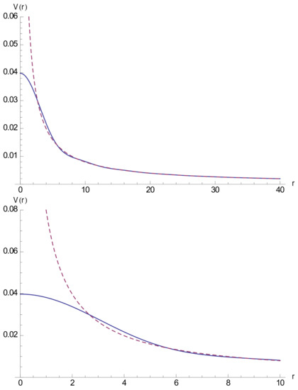
Figure 1.
The potential in (234) for and for unit charges and (solid line) vs. the ordinary potential (dashed line). The right depict details of Planckian regime.
As shown in the figure, contrary to the undeformed Newtonian case, the -deformed potential does not diverge in the short-distance limit. In the zero distance limit, the potential is finite and approaches the Planckian value of . This feature could be interpreted in terms of point-like sources being effectively smoothed out by the UV effects encoded in the -deformation. This is exactly what is realized in the propagation picture (231) outlined above, and it could be interpreted as the manifestation of the long time evoked property of quantum gravity to provide a universal UV regulator in quantum field theory.
Another way of interpreting the short distance behavior of the -deformed potential (234) is to regard it as an indication of an effective dimensional reduction in the UV. In D spacetime dimension, the static potential scales as and thus the finite value of the potential in the UV can be seen as a reduction of the dimension of spacetime down to at short scales. It is interesting to notice that such value agrees with the UV behavior of the spectral dimension studied in [58] for the particular choice of momentum space Laplacian corresponding to the Wick-rotated Casimir
This concludes our brief overview of the basic feature of -deformed field theory.
5. Outlook
Let us close this review by mentioning some of the open problems that the theory of -deformation still faces. On the mathematical side, the major problem is to find out if the quantum R-matrix associated with the -Poincaré algebra exists and, if it does, compute it. Solving this problem is of fundamental relevance for description of the Fock space of -deformed quantum fields and will provide a constructive way to derive the form of multi-particle states and their properties [59,60]. Moreover, the solution of this problem will complete the construction of the relevant quantum group structure of -Poincaré. The problem has been approached, unsuccessfully, in a number of works (see, e.g., [61,62] for a relatively recent attempt).
From the perspective of the physical applications of -deformation, the most urgent question is to firmly establish a link between quantum gravity and the -Poincaré algebra in four physical spacetime dimensions. The first question one should answer is: What is going to be the possible role of the -Poincaré algebra in quantum gravity? One of the possible answers is provided by dimensional analysis. Quantum gravity is characterized by two scales of mass (Planck mass) and length (Planck length), while only one scale is present in -Poincaré. Therefore, one can speculate [39] that the -deformation becomes relevant in the limit of quantum gravity, in which the Planck length is negligible while Planck mass remains finite. In physical terms, this means that the -deformation could describe physical systems whose characteristic size (e.g., impact parameter in the case of scattering) is much larger than the Planck length, while the characteristic energy is still in the order of Planck energy. There is a qualitative argument [19] that such systems can be effectively described by three-dimensional gravity, in which case we know that the deformation is going to emerge. Similarly, one could argue that the vacuum of quantum gravity theory is described by a four-dimensional topological theory [63], which results in effective deformation of spacetime symmetries in a way similar to what happens in the case of three-dimensional gravity [20].
Finally, the -Poincaré algebra serves as one of the most prominent models in the field of quantum gravity phenomenology, and there are various observations which can be used to test the prediction of this model (see the upcoming paper [64] for a comprehensive review).
Author Contributions
All authors contributed equally. All authors have read and agreed to the published version of the manuscript.
Funding
This research received no external funding.
Institutional Review Board Statement
Not applicable.
Informed Consent Statement
Not applicable.
Data Availability Statement
Not applicable.
Acknowledgments
For JKG, this work was supported by funds provided by the National Science Center, project number 2017/27/B/ST2/01902 and 2019/33/B/ST2/00050. This review contributes to the European Union COST Action CA18108 Quantum gravity phenomenology in the multi-messenger approach.
Conflicts of Interest
The authors declare no conflict of interest.
References
- Amelino-Camelia, G. Relativity in space-times with short distance structure governed by an observer independent (Planckian) length scale. Int. J. Mod. Phys. D 2002, 11, 35–60. [Google Scholar] [CrossRef]
- Amelino-Camelia, G. Testable scenario for relativity with minimum length. Phys. Lett. B 2001, 510, 255–263. [Google Scholar] [CrossRef]
- Hossenfelder, S. Minimal Length Scale Scenarios for Quantum Gravity. Living Rev. Rel. 2013, 16, 2. [Google Scholar] [CrossRef] [PubMed]
- Magueijo, J.; Smolin, L. Lorentz invariance with an invariant energy scale. Phys. Rev. Lett. 2002, 88, 190403. [Google Scholar] [CrossRef] [PubMed]
- Magueijo, J.; Smolin, L. Generalized Lorentz invariance with an invariant energy scale. Phys. Rev. D 2003, 67, 044017. [Google Scholar] [CrossRef]
- Lukierski, J.; Ruegg, H.; Tolstoi, A.N.V.N. Q deformation of Poincare algebra. Phys. Lett. B 1991, 264, 331. [Google Scholar] [CrossRef]
- Lukierski, J.; Nowicki, A.; Ruegg, H. New quantum Poincare algebra and k deformed field theory. Phys. Lett. B 1992, 293, 344. [Google Scholar] [CrossRef]
- Lukierski, J.; Ruegg, H.; Zakrzewski, W.J. Classical quantum mechanics of free kappa relativistic systems. Ann. Phys. 1995, 243, 90. [Google Scholar] [CrossRef]
- Lukierski, J.; Ruegg, H. Quantum kappa Poincare in any dimension. Phys. Lett. B 1994, 329, 189. [Google Scholar] [CrossRef]
- Majid, S.; Ruegg, H. Bicrossproduct structure of kappa Poincaré group and noncommutative geometry. Phys. Lett. 1994, 334, 348. [Google Scholar] [CrossRef]
- Kowalski-Glikman, J. Observer independent quantum of mass. Phys. Lett. A 2001, 286, 391–394. [Google Scholar] [CrossRef]
- Bruno, N.R.; Amelino-Camelia, G.; Kowalski-Glikman, J. Deformed boost transformations that saturate at the Planck scale. Phys. Lett. B 2001, 522, 133–138. [Google Scholar] [CrossRef]
- Kowalski-Glikman, J. De sitter space as an arena for doubly special relativity. Phys. Lett. B 2002, 547, 291. [Google Scholar] [CrossRef]
- Kowalski-Glikman, J.; Nowak, S. Doubly special relativity and de Sitter space. Class. Quant. Grav. 2003, 20, 4799. [Google Scholar] [CrossRef]
- Kowalski-Glikman, J.; Nowak, S. Quantum kappa-Poincare algebra from de Sitter space of momenta. arXiv 2004, arXiv:hep-th/0411154. [Google Scholar]
- Born, M. A suggestion for unifying quantum theory and relativity. Proc. R. Soc. Lond. A 1938, 165, 921. [Google Scholar] [CrossRef]
- Majid, S. Meaning of noncommutative geometry and the Planck scale quantum group. Lect. Notes Phys. 2000, 541, 227–276. [Google Scholar]
- Amelino-Camelia, G.; Smolin, L.; Starodubtsev, A. Quantum symmetry, the cosmological constant and Planck scale phenomenology. Class. Quant. Grav. 2004, 21, 3095. [Google Scholar] [CrossRef]
- Freidel, L.; Kowalski-Glikman, J.; Smolin, L. 2 + 1 gravity and doubly special relativity. Phys. Rev. D 2004, 69, 044001. [Google Scholar] [CrossRef]
- Kowalski-Glikman, J.; Starodubtsev, A. Effective particle kinematics from Quantum Gravity. Phys. Rev. D 2008, 78, 084039. [Google Scholar] [CrossRef]
- Cianfrani, F.; Kowalski-Glikman, J.; Pranzetti, D.; Rosati, G. Symmetries of quantum spacetime in three dimensions. Phys. Rev. D 2016, 94, 084044. [Google Scholar] [CrossRef]
- Rosati, G. κ–de Sitter and κ-Poincaré symmetries emerging from Chern-Simons (2+1)D gravity with a cosmological constant. Phys. Rev. D 2017, 96, 066027. [Google Scholar] [CrossRef]
- Freidel, L.; Livine, E.R. 3D Quantum Gravity and Effective Noncommutative Quantum Field Theory. Phys. Rev. Lett. 2006, 96, 221301. [Google Scholar] [CrossRef]
- Freidel, L.; Majid, S. Noncommutative harmonic analysis, sampling theory and the Duflo map in 2+1 quantum gravity. Class. Quant. Grav. 2008, 25, 045006. [Google Scholar] [CrossRef]
- Bais, F.A.; Muller, N.M.; Schroers, B.J. Quantum group symmetry and particle scattering in (2+1)-dimensional quantum gravity. Nucl. Phys. B 2002, 640, 3–45. [Google Scholar] [CrossRef]
- Meusburger, C.; Schroers, B.J. Poisson structure and symmetry in the Chern-Simons formulation of (2+1)-dimensional gravity. Class. Quant. Grav. 2003, 20, 2193–2234. [Google Scholar] [CrossRef]
- Meusburger, C.; Schroers, B.J. The quantisation of Poisson structures arising inChern-Simons theory with gauge group G⋉g*. Adv. Theor. Math. Phys. 2003, 7, 1003–1043. [Google Scholar] [CrossRef]
- Meusburger, C.; Schroers, B.J. Quaternionic and Poisson-Lie structures in 3d gravity: The Cosmological constant as deformation parameter. J. Math. Phys. 2008, 49, 083510. [Google Scholar] [CrossRef]
- Arzano, M.; Kowalski-Glikman, J. Deformations of Space-Time Symmetries. Gravity, Group-Valued Momenta and Non-Commutative Fields; Lecture Notes in Physics; Springer: Berlin/Heidelberg, Germany, 2021. [Google Scholar]
- Weinberg, S. The Quantum Theory of Fields; Cambridge University Press: Cambridge, UK, 1995; Volume 1. [Google Scholar]
- Abraham, R.; Marsden, J.E. Foundation of Mechanics; Benjamin/Cummings Publishing Company: Reading, MA, USA, 1978. [Google Scholar]
- Vilenkin, N.J.; Klimyk, A.U. Representation of Lie Groups and Special Functions; Kluwer Academic Publishers: Dordrecht, The Netherlands, 1993; Volume 3. [Google Scholar]
- Chari, V.; Pressley, A. A Guide to Quantum Groups; Cambridge Uniersity Press: Cambridge, UK, 1994. [Google Scholar]
- Majid, S. Foundations of Quantum Group Theory; Cambridge Uniersity Press: Cambridge, UK, 1995. [Google Scholar]
- Amelino-Camelia, G. Quantum-Spacetime Phenomenology. Living Rev. Rel. 2013, 16, 1–137. [Google Scholar] [CrossRef]
- Arzano, M.; Gubitosi, G.; Magueijo, J.; Amelino-Camelia, G. Anti-de Sitter momentum space. Phys. Rev. D 2015, 92, 024028. [Google Scholar] [CrossRef]
- Kosinski, P.; Lukierski, J.; Maslanka, P.; Sobczyk, J. The Classical basis for kappa deformed Poincare (super)algebra and the second kappa deformed supersymmetric Casimir. Mod. Phys. Lett. A 1995, 10, 2599–2606. [Google Scholar] [CrossRef]
- Borowiec, A.; Pachol, A. Classical basis for kappa-Poincare algebra and doubly special relativity theories. J. Phys. A 2010, 43, 045203. [Google Scholar] [CrossRef]
- Amelino-Camelia, G.; Freidel, L.; Kowalski-Glikman, J.; Smolin, L. The principle of relative locality. Phys. Rev. D 2011, 84, 084010. [Google Scholar] [CrossRef]
- Arzano, M.; Nettel, F. Deformed phase spaces with group valued momenta. Phys. Rev. D 2016, 94, 085004. [Google Scholar] [CrossRef]
- Kirillov, A.A. Elements of the Theory of Representations; Springer: Berlin/Heidelberg, Germany, 1976. [Google Scholar]
- Amelino-Camelia, G.; Arzano, M. Coproduct and star product in field theories on Lie algebra noncommutative space-times. Phys. Rev. D 2002, 65, 084044. [Google Scholar] [CrossRef]
- Daszkiewicz, M.; Imilkowska, K.; Kowalski-Glikman, J.; Nowak, S. Scalar field theory on kappa-Minkowski space-time and doubly special relativity. Int. J. Mod. Phys. A 2005, 20, 4925. [Google Scholar] [CrossRef]
- Freidel, L.; Kowalski-Glikman, J.; Nowak, S. Field theory on kappa-Minkowski space revisited: Noether charges and breaking of Lorentz symmetry. Int. J. Mod. Phys. A 2008, 23, 2687. [Google Scholar] [CrossRef]
- Arzano, M.; Kowalski-Glikman, J.; Walkus, A. Lorentz invariant field theory on kappa-Minkowski space. Class. Quant. Grav. 2010, 27, 025012. [Google Scholar] [CrossRef]
- Arzano, M.; Kowalski-Glikman, J. Non-commutative fields and the short-scale structure of spacetime. Phys. Lett. B 2017, 771, 222–226. [Google Scholar] [CrossRef]
- Arzano, M.; Consoli, L.T. Signal propagation on κ-Minkowski spacetime and nonlocal two-point functions. Phys. Rev. D 2018, 98, 106018. [Google Scholar] [CrossRef]
- Amelino-Camelia, G.; Majid, S. Waves on noncommutative space-time and gamma-ray bursts. Int. J. Mod. Phys. A 2000, 15, 4301–4324. [Google Scholar] [CrossRef]
- Sitarz, A. Noncommutative differential calculus on the kappa Minkowski space. Phys. Lett. B 1995, 349, 42. [Google Scholar] [CrossRef]
- Kowalski-Glikman, J.; Walkus, A. Star product and interacting fields on kappa-Minkowski space. Mod. Phys. Lett. A 2009, 24, 2243. [Google Scholar] [CrossRef]
- Guedes, C.; Oriti, D.; Raasakka, M. Quantization maps, algebra representation and non-commutative Fourier transform for Lie groups. J. Math. Phys. 2013, 54, 083508. [Google Scholar] [CrossRef]
- Arzano, M.; Latini, D.; Lotito, M. Group Momentum Space and Hopf Algebra Symmetries of Point Particles Coupled to 2+1 Gravity. SIGMA Symmetry Integr. Geom. Methods Appl. 2014, 10, 079. [Google Scholar] [CrossRef]
- Groenewold, H.J. On the Principles of elementary quantum mechanics. Physica 1946, 12, 405–460. [Google Scholar] [CrossRef]
- Moyal, J.E. Quantum mechanics as a statistical theory. Proc. Camb. Phil. Soc. 1949, 45, 99–124. [Google Scholar] [CrossRef]
- Arzano, M.; Bevilacqua, A.; Kowalski-Glikman, J.; Rosati, G.; Unger, J. κ-deformed complex fields and discrete symmetries. arXiv 2020, arXiv:2009.03135. [Google Scholar]
- Gubitosi, G.; Arzano, M.; Magueijo, J. Quantization of fluctuations in deformed special relativity: The two-point function and beyond. Phys. Rev. D 2016, 93, 065027. [Google Scholar] [CrossRef]
- Arzano, M.; Gubitosi, G.; Magueijo, J.; Amelino-Camelia, G. Vacuum fluctuations in theories with deformed dispersion relations. Phys. Rev. D 2015, 91, 125031. [Google Scholar] [CrossRef]
- Arzano, M.; Trzesniewski, T. Diffusion on κ-Minkowski space. Phys. Rev. D 2014, 89, 124024. [Google Scholar] [CrossRef]
- Arzano, M.; Marciano, A. Fock space, quantum fields and kappa-Poincare symmetries. Phys. Rev. D 2007, 76, 125005. [Google Scholar] [CrossRef]
- Arzano, M.; Benedetti, D. Rainbow statistics. Int. J. Mod. Phys. A 2009, 24, 4623–4641. [Google Scholar] [CrossRef]
- Young, C.A.S.; Zegers, R. On kappa-deformation and triangular quasibialgebra structure. Nucl. Phys. B 2009, 809, 439–451. [Google Scholar] [CrossRef]
- Young, C.A.S.; Zegers, R. Covariant particle statistics and intertwiners of the kappa-deformed Poincare algebra. Nucl. Phys. B 2008, 797, 537–549. [Google Scholar] [CrossRef]
- Freidel, L.; Starodubtsev, A. Quantum gravity in terms of topological observables. arXiv 2005, arXiv:hep-th/0501191. [Google Scholar]
- Quantum Gravity Phenomenology in the Multi Messenger Approach. Prog. Part. Nucl. Phys. to appear.

Publisher’s Note: MDPI stays neutral with regard to jurisdictional claims in published maps and institutional affiliations. |
© 2021 by the authors. Licensee MDPI, Basel, Switzerland. This article is an open access article distributed under the terms and conditions of the Creative Commons Attribution (CC BY) license (https://creativecommons.org/licenses/by/4.0/).