A Commodity Classification Framework Based on Machine Learning for Analysis of Trade Declaration

Abstract

Text, voice, images and videos can express some intentions and facts in daily life. By understanding these contents, people can identify and analyze some behaviors. This paper focuses on the commodity trade declaration process and identifies the commodity categories based on text information on customs declarations. Although the technology of text recognition is mature in many application fields, there are few studies on the classification and recognition of customs declaration goods. In this paper, we proposed a classification framework based on machine learning (ML) models for commodity trade declaration that reaches a high rate of accuracy. This paper also proposed a symmetrical decision fusion method for this task based on convolutional neural network (CNN) and transformer. The experimental results show that the fusion model can make up for the shortcomings of the two original models and some improvements have been made. In the two datasets used in this paper, the accuracy can reach 88% and 99%, respectively. To promote the development of study of customs declaration business and Chinese text recognition, we also exposed the proprietary datasets used in this study.

1. Introduction

Commodity declaration is an indispensable process in the import and export trade. With the development of e-commerce and logistics technology, the number of commodity import and export trade has increased rapidly. Due to different tax rates, each type of commodity needs to be divided into different Harmonization System Code (HS-code). It is a system for quantitative management of entry-exit tariff rates of various products [1]. For a commodity declaration process, three necessary elements need to be submitted, commodity names, commodity descriptions and commodity HS-codes. Generally speaking, the name and description of a trade commodity are obvious. However, to fill in the HS-code, salespeople need a lot of professional business knowledge and consult many relevant manuals. There are 98 sections and over ten thousand different HS-codes [2]. Consequently, a workload of commodity classification in a commodity declaration is tedious and huge.

As for the commodity declaration application, there is only a limited number of studies. Most of the declaration systems help people declare HS-code through text similarity with historical data, which can identify correct HS-code with pinpoint accuracy if the commodity occurs during the historical trade. However, new goods never appearing are difficult to be directly assigned to the correct code. Then, we consider utilizing machine learning (ML)-based methods to complete the HS-code declaration process. ML models are widely used in computer vision (CV), natural language processing (NLP) and user behavior prediction [3]. It is universally known that CNN-based, Long short-term memory (LSTM)-based and transformer-based [4] models make great achievements in CV and NLP. In user behavior prediction fields, there are also some mature applications. For instance, Sarker et al. [5] formulate the problem of building a context-aware predictive model based on Decision Tree (DT) for predicting user diverse behavioral activities with smartphones. Zeng et al. [6] proposed an ML framework for predicting users’ behavior interests. These studies inspire us to focus on the ML-based model to address the problem of declaration behavior identification.

In fact, the HS-code identification can be regarded as a classification task. Users should find the correct HS-code according to the properties of a commodity when declaring. Some experts attempt to improve the HS-code classification precision based on some ML models [7,8]. From the viewpoint of results, these methods have made some progress, but there is still a lot of room for improvement in accuracy. There are more than 10,000 different codes. It is difficult to seek out the correct code directly by a 10,000-classifier. In this paper, we split HS-code into multiple levels and built a classification framework based on ML. The results show that our methods perform well in two private Chinese declaration datasets. The key contributions of the presented work are the following:

(1)

This paper proposed a commodity classification framework based on ML for trade declaration. It contains hierarchical splitting of object coding, some improvement of CNN-based and Bert-based models, and commodity analysis. Each classification model achieved good results on the two declaration datasets.

(2)

We employ the symmetrical decision fusion of two classification models for HS-code identification. The proposed fusion methods are more accurate than a single one on our datasets.

(3)

We expose two Chinese commodity declaration datasets used in this paper. One contains more than 220,000 samples collected from some cooperative companies and websites, the other is gathered from a third party company whose source is different from the first one.

The rest of the paper is organized as follows: Section 2 introduces some methods and applications related to this paper. Section 3 describes the overview HS-code classification framework for commodity declaration. In Section 4, we depict the proposed methods and models. Section 5 shows the experiment process and results. Section 6 concludes the main idea of this paper and introduces the future work.

2. Literature Review and Related Work

The research of HS-code classification helps to simplify the users’ operation in the process of customs declaring. In the beginning, people complete the HS-code classification by manual design with tax regulations. We have investigated a lot of literatures about HS-code classification work. So far, there are only a few automatic classification methods of HS-code in the actual customs declaring scene, especially for Chinese models. We undertake an in-depth literature review of this topic over the past five years, and then introduce some related technology in other similar fields.

Lee et al. [9] proposed an LSTM-based HS-code identification method and the accuracy reached 66% with 230 target classes. Spichakova and Haav [10] introduced a novel combined similarity measure based on cosine similarity of texts and semantic similarity of HS-codes calculated according to their taxonomy. Ref. [11] proposed a CNN-based HS items classification model with the accuracy of 73%. Kyung-Ah et al. [12] designed an apparatus for searching the HS-code of a product, which can search code by keywords. Ding et al. [13] adopted Background Nets approach and use multi-step association to help categorization for short record description. Reid [14] built a system with a harmonization server receiving and processing customer information and product information through which they complete HS-code classification. Chong-Jian et al. [15] analyzed a DL-based model and a maximum entropy-based model on HS-code classification and concluded the DL-based one has a better performance. Although these methods are based on practical application scenarios, their application scope is relatively small and the accuracy is relatively low. At the same time, there is little research on Chinese commodity HS-code classification, and there are no relevant public data. Consequently, we extended our vision to other research methods in similar fields.

Users always identify the commodity HS-code by goods description information, which can be realized by text classification in NLP with ML and deep learning (DL) methods. K-Nearest Neighbor (KNN) is a traditional ML method based on a vector space. Li et al. [16] proposed a text classification method Ni-KNN. This method calculates the similarities by considering the interaction and coupling relationship between documents and within documents, so as to solve the problem that the traditional KNN classification algorithm ignores the rough similarity calculation between them. Goudjil et al. [17] proposed a novel active learning method for text classification. They use the posterior probability provided by multi class SVM classifier to select a batch of information samples, and then the experts label these samples manually, which can significantly reduce the labeling work. Random Forest (RF) is also a traditional ML method that can complete the work on the text classification. Xu et al. [18] proposed a new feature weighting method and tree selection method, which makes the RF framework suitable for multi-topic text document classification. Tree boosting is an efficient and widely used machine learning method (Chen and Guestrin [19]). Zhang and Zhan [20] extract features from pre-processed samples by TF-IDF, then training models based on XGBoost. In addition to the structure of the algorithm, the effect of traditional ML algorithms depends on features engineering, which usually requires a lot of professional business experience.

DL automatically extracts important features from text, which solves the limitation of manual feature selection. Recently, text classification methods based on neural networks have been widely concerned because of their excellent performance in various situations [21,22,23,24]. At present, there are many improvements in word embedding and CNN model architecture. Considering that the same word usually has different importance in documents with different category labels, Guo et al. [25] proposed a word-weighted scheme combined with word embedding. Each word is given multiple weights that are applied to the word embedding, and transformed features are input into the multi-channel CNN model to predict the label of the sentence. Yao et al. [26] proposed a novel Chinese fine-grained named entity recognition(NER) method based on Bert and LSTM. Jang et al. [27] used Word2vec to learn the semantic information between words, and give low weight value to irrelevant text content, to reduce the impact of useless data on model training and improve the classification performance. CNN can only extract local features, which are usually more suitable for short text. In 2018, Google released the Bert model (Devlin et al. [28]), using Bert pre-trained language model to fine tune the downstream text classification tasks which achieved excellent performance. The automatic classification of HS-codes can reduce labor consumption. The main goal is to achieve the prediction of trade declaration behavior through historical data of customs declarations. In order to apply HS-code classification to the actual scene, we collect a large number of historical data, and choose to carry out experiments based on Bert and CNN models to get optimization models.

3. Overview of the Framework

This paper targets helping people to complete the trade declaration automatically. Figure 1 depicts the process of declaration with data processing, modeling and classification strategy. As shown in the figure, part A is the original data that consists of training data and their labels. Part B describes the process of data processing. From part C and D, we define the declaration process as a classification task. Our aim is to get the correct 10-digit HS-code. Since the number of HS-code is too large and data distribution is unbalanced in each code, we split the code into multiple. According to the results, the split method improve the separability of a single model. From a business perspective, the establishment of HS-code is completed through different chapters, sections and items by each HS-code digital. HS-code is divided into 22 categories and 98 chapters by the first 2 digits. The third and forth digits determine its section and the fifth and sixth show its items. The rest digits are the classification criteria for goods defined by countries. The original Chinese text data are transferred to vectors and sent to the classifiers based on ML. Some traditional ML models, neural network-based models and fusion models are used in this paper. Then, the final intact HS-code is obtained by multi-layer superposition.

As for the trade declaration process, our framework completely replaces the manual retrieval process that shows as the red dotted box in part E and F. When handling the commodity declaration data that did not occur before, we do not need to consult datum again. The experiments proved that the automatic classification process can improve the identification efficiency and classification accuracy compared with other existing methods. An accuracy of over 99% can be achieved in our dataset.

4. Models and Methods

In this section, we will introduce the model structure in detail. In the experiment, four key models based on DL and a symmetrical decision fusion model are proposed in trade declaration task. Since the model is based on CNN and Bert, these models are christened as HSBert, HSCNN and HSnet. Then, we introduce a symmetrical decision fusion method of HSBert and HSnet. In addition, we also use several traditional ML models as a comparison, such as Random Forest (RF) [18], Support Vector Machines (SVM) [29] and XGBoost [20]. SVM finds the optimal separation hyperplane from the feature space to realize the classification function based on the theory of structural risk minimization. XGBoost is an ensemble learning method based on cart tree and gets the classification result by continuous iterative learning. RF uses bootstrap-resampling technology to select n samples to form a random forest and it is determined by the number of votes of the classification tree. These traditional ML methods are basically used directly and will not be described in great detail below in this section.

4.1. HSBert

We use parameters of pre-trained Bert model as HSBert’s initial parameters, and then fine tune the model using the history data in the actual scene (Devlin et al. [28]). Figure 2 shows the structure of the overall model. HSBert is composed of embedding layer, Bert encoder layer and classification layer.

To distinguish the beginning of a sentence from the segmentation between two sentences, we introduced two special notation[CLS] and[SEP] (Sun et al. [30]). The same tokens combined by multiple words in Chinese text usually have different meanings. Therefore, we use WordPiece that can split Chinese sentences into multiple words (Wu et al. [31]). It is beneficial to the semantic learning of polysemous and out-of-word (OOV) words. Sometimes, the importance of the same token in different sentences is also different, and token type embedding can solve the problem. Bert is a multi-layer bidirectional Transformer (Vaswani et al. [32]) based language representation model, which means it cannot obtain the sequence information of the token. Therefore, position Embedding is introduced to add location information to make up for that. The Embedding layer is used to represent the input text that composition is as follows:

$$E_{input}=E_{word\_embedding}+E_{token\_type\_embedding}+E_{position\_embedding},$$

(1)

where $E_{input}$ is the final vector embedding which can be input into the model, $E_{word\_embedding}$ is word embedding, $E_{token\_type\_embedding}$ is token type embedding, $E_{position\_embedding}$ is position embedding.

The Bert Encoder layer is composed of a stack of N identical Transformer blocks, We denote the Transformer block as $T\left(h\right)$, in which h represents the hidden vector. Mini batch is usually used in the process of self-attention calculation. The model’s input dimension is $B\times S$, which B is the size of a batch and S is the length of a sentence. The mini batch is composed of sentences with different lengths, so we set a max sequence length parameter. If a sentence in a batch exceeds max sequence length, the excess length will be cut off. Similarly, the sentences that are not long enough is filled with 0. This process is padding. However, the part filled with 0 will also participate in self-attention, so attention mask is used to solve this problem. Attention mask can make the invalid part not participate in the calculation. The detailed operations of Bert Encoder layer are as follows:

$$h_0=A_{mask}+E_{input}$$

(2)

$$h_n=T\left(h_{(n-1)}\right),n\in [1,N],$$

(3)

where $A_{mask}$ is the matrix of a one-hot vector, which represents masked attention. $h_n$ is the hidden state vector at n-th layer.

The Classification layer is a fully connected layer with dropout mechanism and softmax function:

$$p_{class-i}=softmax(W_c{h}_{cls}+b_c),$$

(4)

where $W_c$, $b_c$ are learnable parameters, $h_{cls}$ is the first word which contains the semantic information of the whole sentence. The softmax function can get probability of i-th class $p_{class-i}$.

4.2. HSCNN-Rand and HSCNN-Static

We also use convolution neural network to design a classification model, which is mainly composed of Embedding layer, Convolution layer and Classification layer.

The Embedding layer is to match each word in the input text with the corresponding word vector. From the Figure 3, we use two embedding ways: Random initialization and Word2vec (Ma and Zhang [33]), so models are divided into HSCNN-rand and HSCNN-static. Word2vec uses the data in the dataset to get a word embedding dictionary, in which each word corresponds to a word embedding by training. A sentence of length n (with padding) is represented as:

$$x_{1:n}=x_1\oplus x_2\oplus \cdots \oplus x_n$$

(5)

where ⊕ is the concatenation operator. $x_i$ is word embedding of x, which $x_i\in R^{1k}$.

We use three different sizes of convolution kernels to extract features from word embedding matrix in order to get more different feature combinations, and then select the most important features by using max pooling.. The procedure can be represented as follows:

$$c_{1i}=f\left(w_1·x_{i:i+h-1}+b_1\right)$$

(6)

$$c_{2i}=f\left(w_2·x_{i:i+h-1}+b_2\right)$$

(7)

$$c_{3i}=f\left(w_3·x_{i:i+h-1}+b_3\right),$$

(8)

where $w_1,w_2,w_3\in \left\{R^{h1*k},R^{h2*k},R^{h3*k}\right\}$ are three different size of convolution kernels. $b_1$, $b_2$, $b_3$ are bias. These convolution kernels are applied to each possible window of words in the sentence $\left\{x_{1:h},x_{2:h+1},\cdots ,x_{n-h+1:n}\right\}$ to produce three feature map:

$$C_1=\left[c_{11},c_{12},\cdots ,c_{n-h1+1}\right]$$

(9)

$$C_2=\left[c_{21},c_{22},\cdots ,c_{n-h2+1}\right]$$

(10)

$$C_3=\left[c_{21},c_{22},\cdots ,c_{n-h3+1}\right].$$

(11)

Then apply a max pooling operation to get the most important feature:

$$c_1=max\left(C_1\right)$$

(12)

$$c_2=max\left(C_2\right)$$

(13)

$$c_3=max\left(C_3\right)$$

(14)

After this, using concatenation operator to gather all important features as the sentence’s semantic vector. We can see that the structures of $c_1$, $c_2$ and $c_3$ have a high degree of symmetry with the dimension of $5\times 5$:

$$c=c_1\oplus c_2\oplus c_3.$$

(15)

The classification layer uses a linear function to map all HS-code classes, and applys dropout mechanism to avoid overfitting:

$$p_{\mathrm{class}-i}=softmax\left(w_{c}c+b_c\right),$$

(16)

where $w_c,b_c$ are learnable parameters, and using softmax function can get probability of i-th class $p_{class-i}$.

4.3. HSNet

The HSNet model’s structure design is shown in Figure 4. Its Embedding layer includes HSBert’s Embedding and Bert Encoder layer, using different sizes of convolution kernels to extract more important semantic vector like HSCNN-rand’s Convolution layer. The process can be expressed as:

$$\left(h_1,h_2,\cdots ,h_n\right) = Bert\_Encoder\left(E_{\mathrm{input}}\right)$$

(17)

$$c_{ij}=f\left(w_i·{\hslash }_{j:j+h-1}+b_i\right),i\in [1,k]$$

(18)

$$c=c_1\oplus c_2\oplus \cdots \oplus c_k,$$

(19)

where $\mathrm{Bert\_Encoder}$ represents the HSBert’s embedding layer and Bert encoder layer, and $E_{input}$ represents input embedding. $h_i$, $i\in [1,n]$ are hidden vectors obtained from Bert Encoder layer. The Convolution layer has k different sizes of convolution kernels. $w_i$ and $b_i$ are parameters of convolution layer, and c represent hidden vector after convolution layer.

The classification layer is also the same as HSCNN-rand, which can reference Equation (16).

4.4. Symmetrical Decision Fusion Model

Although the above models performed well in the experiments, we find that the performances of a model on different datasets are different. HSBert is the best model on HS-Dataset1, but the performance of it is worse than HSNet on HS-Dataset2, which enlightens us to consider whether we can get better results from the fusion of the two models. Generally speaking, there are three fusion strategies, namely early data fusion, feature fusion and symmetrical decision fusion [34]. In this paper, since there are only one type of data source, we will not consider the data fusion and feature fusion. Consequently, we design a symmetrical decision fusion framework for the task shown in Figure 5.

As Figure 5 shows, raw data is used twice on two different classifiers to extract more features. We select HSBert and HSNet as the training models that perform best on HS-Dataset1 and HS-Dataset2 respectively. After the classifiers calculates the probability that the sample is divided into each target, we take the prediction probability of the two models as the symmetrical prediction weight of each class. Then the two weights are added to get the final fusion prediction probability. We call this process as symmetrical decision fusion, since the fusion process of this method takes place after the classification and prediction stage of the classifier. The benefit is that the former model and the training process are relatively independent, and the influence between the two models is relatively small.

5. Experiments and Results

5.1. Datasets

We collect real historical data to train and evaluate the model for applying our models to the customs declaring scene. We select 84 chapter that is representative and have enough samples as the research object. HS-codes are usually 10-bit codes, and it is hard to be classified directly for their large number of categories. Considering reducing the complexity of the experiment implementation and improving the effect of classification, the classification experiments of 2-bit to 4-bit, 4-bit to 6-bit and 6-bit to 8-bit are carried out from the perspective of hierarchy. Two Chinese commodity declaration datasets used in this paper are HS-Dataset1 and HS-Dataset2. Data details of the two datasets are shown in

Table 1. Basic information and distribution of two datasets.

Dataset	HS-Dataset1			HS-Dataset2
Hierarchy	2 bit to 4 bit	4 bit to 6 bit	6 bit to 8 bit	2 bit to 4 bit	4 bit to 6 bit	6 bit to 8 bit
Class num	19	66	105	8	12	15
Train	181,213	161,419	121,703	-	-	-
Dev	45,315	40,392	30,480	-	-	-
Test	45,315	40,392	30,480	8899	8773	8730

.

HS-Dataset1 contains 226,528 samples collected from some cooperative companies and websites, which are divided into 181,213 train samples and 45,315 test samples according to the proportion of 8:2. After sample filtering, there are 19 categories of 4-bit codes, 66 categories of 6-bit codes and 105 categories of 8-bit codes. The maximum length of the sample is 126 words and the minimum length is three words.

HS-Dataset2 contains 8899 samples gathered from a third party company, which are used as test samples. After sample filtering, there are eight categories of 4-bit codes, 12 categories of 6-bit codes and 15 categories of 8-bit codes. The maximum length of the sample is 142 words and the minimum length is 26 words.

Table 2. Examples of data samples in HS-Dataset1 and HS-Dataset2.

Dataset	Data Sample
HS-Dataset1	落地扇,家用|落地扇|70W/82W
	通讯机箱配件(风扇),用于通讯机箱散热用|镶嵌在机箱内部
	风扇配件,风扇用|无型号|铁|塑胶|网扣开关旋钮底盘外管网束摇头座
	落地扇,降温纳凉用|落地扇
	电子产品散热风扇,电子产品散热|螺丝固定
HS-Dataset2	离心通风扇,境内收购品牌|不适用于进口报关单|离心通风扇|2.52W|TOSHIBA牌|C-E05C
	轴流风扇,境外品牌(其他)|不适用于进口报关单|打印机散热用|轴流风扇|2.4W|NMB牌|无型号
	轴流风扇,无品牌|不适用于进口报关单|散热用|小型风扇|3.2W|无品牌|无型号
	离心通风扇,境外品牌(其他)|不适用于进口报关单|嵌入式|2.52W|TOSHIBA牌|C-E05C
	离心通风扇,境内收购品牌|不适用于进口报关单|离心通风扇|3W|TOSHIBA牌|C-E02C

depicts some samples of raw data in Chinese and

Table 3. Examples of data samples in HS-Dataset1 and HS-Dataset2, the English explanation for Table 2.

Dataset	Data Sample
HS-Dataset1	pedestal fan, household|pedestal fan|70 W/82 W
	Communication box accessories (fan), Used for cooling communication case|Embedded in the chassis
	Fan accessories, fan with|no model|iron|plastic|net button switch knob chassis outer pipe
	bundle shaking head seat
	pedestal fan, For cooling|pedestal fan
	Cooling fan for electronic products, Heat dissipation of electronic products|Screw fixation
HS-Dataset2	Centrifugal ventilation fan, Domestic brand acquisition|Not applicable to import declaration
	|Centrifugal ventilation fan|2.52 W|TOSHIBA brand|C-E05C
	Axial fan, Foreign brands (others)|not applicable to import declaration|printer cooling
	|axial fan|2.4 W|NMB|no modell
	Axial fan, No brand|not applicable to import declaration|cooling|small fan|3.2 w
	|no brand|no model
	Centrifugal ventilation fan, Overseas brand (others)|not applicable to import declaration
	|embedded|2.52 w|Toshiba|c-e05c
	Centrifugal ventilation fan, Domestic acquired brand|not applicable to import customs declaration
	|centrifugal fan|3 W|TOSHIBA brand|C-E02C

depicts these samples in English that is the explanations for Table 2. We have made the datasets publicly available for follow-up researchers to continue their related work on commodity trade declaration [35].

5.2. Implementation Details

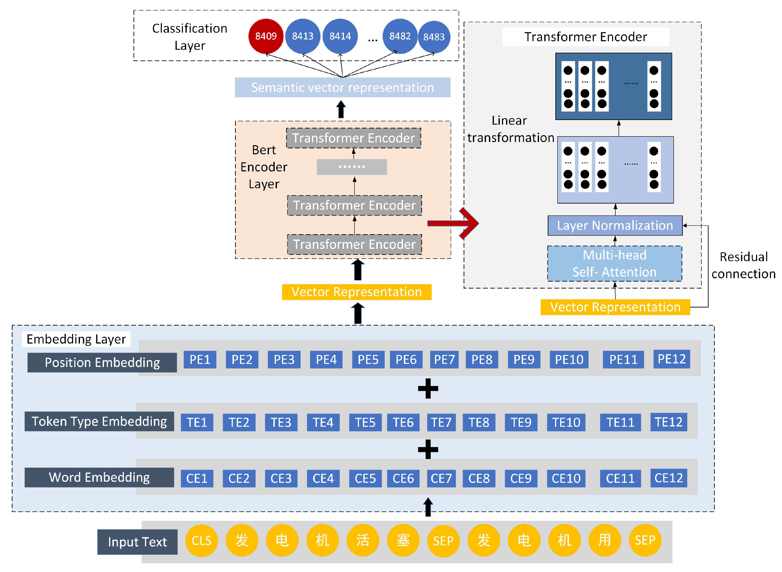
HSBert is composed of embedding layer, Bert encoder layer and classification layer. We use Chinese pre-trained model of Bert to initial it (Devlin et al. [28]). The vocabulary size of the pre-training model is 21,128. The embedding layer includes three kinds of embedding, namely embedding, position embedding and token type embedding. The three types of embedding are set to 768 dimensions. The Encoder layer includes 12 transformer’s encoder layers, and each layer adopts multi-headed attention mechanism, in which the number of self-attention head is 12. The pooling layer is a linear map function that collects the hidden state corresponding to the first token, and then sets a Tanh function [36] to activate. The Classification layer is a fully connected layer. There is a dropout layer with a rate of 0.1 in front of the Classification layer to avoid overfitting (Krizhevsky et al. [37]). The maximum sentence length of the input model is set to 128, and the batch size is set to 16. The model is trained using BertAdam with an initial learning rate of $5\times {10}^{-5}$ which can be optimized by a warmup mechanism (He et al. [38]).

HSCNN-rand and HSCNN-word2vec consist of embedding layer, convolutional layer and classification layer. The embedding layer’s word embedding is set to 128 dimensions. The convolution layer consists of three different one-dimensional convolution kernels, whose sizes are 1, 3 and 5 respectively, and the number of output channels is set to 256. The classification layer is a fully connected linear mapping layer. There is a dropout layer with a rate of 0.2 in front of the classifier layer to avoid overfitting (Krizhevsky et al. [37]). The input of the model is a sentence with a fixed length of 64, and the batch size is set to 16. The model is trained using Adam [39] with an initial learning rate of $1\times {10}^{-3}$.

HSNet is a combination of Bert and CNN which consists of Embedding layer, Convolution layer and Classification layer. The Embedding layer’s sentence embedding is set to 128 dimensions. The convolution layer and the Classification layer are the same as HS-CNN. In order to avoid overfitting, there is a dropout layer with a rate of 0.2 in front of the classifier layer. The input of the model is a sentence with a fixed length of 64, and the batch size is set to 16. The model is trained using Adam with initial learning rate of $1\times {10}^{-3}$.

5.3. Evaluation Metrics

We use Accuracy(Acc), Precision (Prec), Recall (Rec) and F1-score to calculate model results. In order to evaluate the classification effect more objectively, Weighted F1 and Averaged F1 are obtained by weighting F1-score with the number of samples and categories. The details of evaluation metrics are as follows.

Figure 6 is a confusion matrix. Each column of confusion matrix represents the prediction category, and the total number of each column represents the number of data predicted as the category; each row represents the real belonging category of data, and the total number of data in each row represents the number of data instances of the category. Each part is explained as follows:

TP: The actual sample class is positive, and the prediction result of the model is also positive.

TN: The actual sample class is negative, and the prediction result of the model is also negative.

FP: The actual sample class is positive, and the prediction result of the model is also negative.

FN: The actual sample class is negative, and the prediction result of the model is also positive.

Accuracy: The proportion of the correct samples predicted by model among the total samples. The calculation is shown in Equation (20):

$$\mathrm{Accuracy}=\frac{\mathrm{TP}+\mathrm{TN}}{\mathrm{TP}+\mathrm{FN}+\mathrm{FP}+\mathrm{TN}}$$

(20)

Precision: The proportion of the positive samples predicted by the model correctly among the total positive samples. The calculation is shown in Equation (21):

$$\mathrm{Precision}=\frac{\mathrm{TP}}{\mathrm{TP}+\mathrm{FP}}$$

(21)

Recall: The proportion of the the positive samples predicted by the model correctly among the total positive samples predicted by the model. The calculation is shown in Equation (22):

$$\mathrm{Recall}=\frac{\mathrm{TP}}{\mathrm{TP}+\mathrm{FN}}$$

(22)

F1-score: The F1 score is a weighted average of accuracy and recall. The calculation is shown in Equation (23):

$$\mathrm{F}1\text{-}\mathrm{score}=\frac{2*\mathrm{Precision}*\mathrm{Recall}}{\mathrm{Precision}+\mathrm{Recall}}.$$

(23)

Weighted F1: Weighted F1 is obtained by weighting the F1-score with the proportion of different categories of samples to the total number of samples. The calculation is shown in Equation (24):

$$\mathrm{Weighted}\mathrm{F}1=\sum \frac{\mathrm{sample}{}_i}{{\sum }_1^n\mathrm{sample}{}_j}*F{1}_i,$$

(24)

where $\mathrm{sample}{}_i$, $i\in [1,n]$ represents number of i-sample.

Averaged F1: Averaged F1 is obtained by weighting the F1-score with the number of categories of samples. The calculation is shown in Equation (25):

$$\mathrm{Averaged}\mathrm{F}1=\frac{1}{\mathrm{categories}\_\mathrm{num}}\sum F{1}_i,$$

(25)

where $\mathrm{categories}\_\mathrm{num}$ is number of categories.

5.4. Results and Discussion

This section shows the HS-code classification results of all models described in Section 4. We compared the performance of different models. Due to the space limitation, we selected some representative results to explain.

Firstly, we concluded the classification results of all levels of HS-codes in

Table 4. Three levels’ results of HSBert and Fusion Model on two datasets. (a) Three levels’ results of HSBert on HS-Dataset1 and HS-Dataset2. (b) Three levels’ results of Fusion Model on HS-Dataset1 and HS-Dataset2.

(a)
Dataset	Metrics	2 bit to 4 bit	4 bit to 6 bit	6 bit to 8 bit	Total
HS-Dataset1	Acc	0.9465	0.9654	0.9540	0.8718
	Prec	0.9549	0.9729	0.9558	0.8881
	Rec	0.9517	0.9725	0.9551	0.8840
	Weighted F1	0.9531	0.9724	0.9534	0.8837
	Averaged F1	0.9379	0.9421	0.8334	0.7364
HS-Dataset2	Acc	0.9970	0.9999	0.9953	0.9924
	Prec	0.9988	0.9999	0.9937	0.9925
	Rec	0.9971	0.9999	0.9953	0.9924
	Weighted F1	0.9979	0.9999	0.9943	0.9922
	Averaged F1	0.8510	1.0000	0.8393	0.7143
(b)
Dataset	Metrics	2 bit to 4 bit	4 bit to 6 bit	6 bit to 8 bit	Total
HS-Dataset1	Acc	0.9458	0.9655	0.9564	0.8735
	Prec	0.9512	0.9730	0.9562	0.8851
	Rec	0.9529	0.9729	0.9574	0.8877
	Weighted F1	0.9520	0.9728	0.9554	0.8849
	Averaged F1	0.9381	0.9441	0.8388	0.7430
HS-Dataset2	Acc	0.9986	0.9999	0.9964	0.9951
	Prec	0.9992	0.9999	0.9940	0.9933
	Rec	0.9987	0.9999	0.9964	0.9952
	Weighted F1	0.9989	0.9999	0.9952	0.9942
	Averaged F1	0.9897	1.0000	0.8669	0.8580

. They consist of 2-bit to 4-bit level, 4-bit to 6-bit level and 6-bit to 8-bit level. Table 4 shows the evaluation indexes of the single model HSBert and the Fusion model on HS-Dataset1 (Table 4a) and HS-Dataset2 (Table 4b). The Acc, Prec, Rec and Weighted-F1 of HS-Dataset1 attained over 95% in each level, and the comprehensive results of the three levels are over 85%. Averaged-F1 is slightly lower than others. This is due to the imbalanced data in each category. The experiment on HS-Dataset2 indicates a better performance that every metric except Averaged-F1 can reach a high index about 99% in each level.

Comparing the comprehensive performance of the two models, the Fusion Model is slightly higher than HSBert. It proves the effectiveness of taking the prediction probability of HSBert and HSNet models as the prediction weight of each category. From the perspective of metrics, Fusion Model can make better decisions than HSBert. HSBert and Fusion Model all achieved excellent results in HS-Dataset2. We try to consider from the perspective of the original data specification, and find that the latter is more standardized from Table 2 and Table 3, so we speculate that our model can achieve better results on the standardized data. The more standard the data format is, the better performance the model gets. It also explains why the model can do much better for practical use when the data quality is better.

Table 5. The number of class of the two HS-codes 84145990 and 84799090 at each level.

HS-Code	2 bit to 4 bit	4 bit to 6 bit	6 bit to 8 bit
84145990	19	4	2
84799090	19	3	3

shows the number of categories of HS-code 84145990 and 84799090 in each level.

Table 6. The Prec, Rec and F1 of compared models of HS-codes ‘84145990’ on two datasets. Total metrics is marked by *. (a) The Prec, Rec and F1 of compared models of HS-codes ‘84145990’ on HS-Dataset1. (b) The Prec, Rec and F1 of compared models of HS-codes ‘84145990’ on HS-Dataset2.

84145990	Metrics	HSBert	HSNet	Fusion Model	HSCNN-Rand	SVM	XGBoost
(a)
84 -> 8414	Prec	0.9430	0.9219	0.9385	0.9198	0.9300	0.8630
	Rec	0.9498	0.9264	0.9510	0.9462	0.9100	0.8759
	F1	0.9464	0.9241	0.9447	0.9328	0.9200	0.8694
8414 -> 841459	Prec	0.9148	0.9046	0.9076	0.9104	0.8865	0.8688
	Rec	0.9052	0.9010	0.9052	0.8828	0.9052	0.8894
	F1	0.9100	0.9028	0.9064	0.8964	0.8958	0.8790
841459 -> 84145990	Prec	0.9517	0.9576	0.9592	0.9747	0.9300	0.9556
	Rec	0.9890	0.9937	0.9952	0.9670	0.9100	0.9796
	F1	0.9700	0.9753	0.9769	0.9708	0.9200	0.9674
84 -> 84145990	Prec *	0.8211	0.7987	0.8171	0.7871	0.7871	0.7166
	Rec *	0.8504	0.8295	0.8569	0.8163	0.8147	0.7632
	F1 *	0.8354	0.8138	0.8366	0.8014	0.8006	0.7394
(b)
84 -> 8414	Prec	1.0000	1.0000	1.0000	1.0000	0.9881	0.9932
	Rec	1.0000	1.0000	1.0000	1.0000	0.9076	0.9827
	F1	1.0000	1.0000	1.0000	1.0000	0.9461	0.9879
8414 -> 841459	Prec	1.0000	1.0000	1.0000	1.0000	1.0000	0.8688
	Rec	1.0000	1.0000	1.0000	1.0000	0.9239	1.0000
	F1	1.0000	1.0000	1.0000	1.0000	0.9604	0.9976
841459 -> 84145990	Prec	1.0000	1.0000	1.0000	1.0000	0.8661	0.9556
	Rec	1.0000	1.0000	1.0000	1.0000	1.0000	0.9796
	F1	1.0000	1.0000	1.0000	1.0000	0.9283	0.9674
84 -> 84145990	Prec *	1.0000	1.0000	1.0000	1.0000	0.8559	0.9572
	Rec *	1.0000	1.0000	1.0000	1.0000	0.8385	0.9569
	F1 *	1.0000	1.0000	1.0000	1.0000	0.8436	0.9570

depicts results of different models. Combining the results of Table 4, Table 6 and class number of each level in Table 5, it can be concluded that results of 6-bit to 8-bit are much better than 2-bit to 4-bit and 4-bit to 6-bit. It shows that with the increasing of the number of class, the models’ performance will also be affected, which also proves the practicability and superiority of hierarchical experiment of HS-code proposed by us.

Then, in order to observe the HS-code classification results output from each model and compare their differences, we randomly select the outputs of two HS-code ‘84145990’ and ‘84799090’ in Table 6 and

Table 7. The Prec, Rec and F1 of compared models of HS-codes ‘84799090’ on two datasets. Total metrics is marked by *. (a) The Prec, Rec and F1 of compared models of HS-codes ‘84799090’ on HS-Dataset1. (b) The Prec, Rec and F1 of compared models of HS-codes ‘84799090’ on HS-Dataset2.

84799090	Metrics	HSBert	HSNet	Fusion Model	HSCNN-Rand	SVM	XGBoost
(a)
84 -> 8479	Prec	0.8660	0.7467	0.8345	0.8193	0.6300	0.6782
	Rec	0.8207	0.7906	0.8235	0.8399	0.8600	0.7556
	F1	0.8427	0.7680	0.8290	0.8294	0.7300	0.7148
8479 -> 847990	Prec	0.9818	0.9756	0.9803	0.8863	0.9466	0.9201
	Rec	0.9718	0.9711	0.9734	0.9679	0.9281	0.9359
	F1	0.9768	0.9733	0.9768	0.9253	0.9373	0.9280
847990 -> 84799090	Prec	0.9926	0.9934	0.9934	0.9875	0.9886	0.9798
	Rec	0.9942	0.9950	0.9942	0.9721	0.9975	0.9967
	F1	0.9934	0.9942	0.9938	0.9797	0.9930	0.9882
84 -> 84799090	Prec *	0.8440	0.7987	0.8127	0.7171	0.5896	0.6115
	Rec *	0.7931	0.8295	0.7970	0.7903	0.7962	0.7049
	F1 *	0.8178	0.8138	0.8048	0.7518	0.6795	0.6556
(b)
84 -> 8479	Prec	0.9914	0.9956	0.9956	0.8369	0.0298	0.1209
	Rec	1.0000	0.9956	1.0000	1.0000	1.0000	0.9307
	F1	0.9956	0.9956	0.9978	0.9112	0.0579	0.2140
8479 -> 847990	Prec	1.0000	1.0000	1.0000	1.0000	1.0000	1.0000
	Rec	1.0000	1.0000	1.0000	1.0000	0.1101	0.3898
	F1	1.0000	1.0000	1.0000	1.0000	0.1984	0.5609
847990 -> 84799090	Prec	1.0000	1.0000	1.0000	1.0000	1.0000	1.0000
	Rec	1.0000	1.0000	1.0000	1.0000	1.0000	1.0000
	F1	1.0000	1.0000	1.0000	1.0000	1.0000	1.0000
84 -> 84799090	Prec *	0.9914	0.9956	0.9956	0.8369	0.0298	0.1209
	Rec *	1.0000	0.9956	1.0000	1.0000	0.1101	0.3628
	F1 *	0.9956	0.9956	0.9978	0.9112	0.0115	0.1200

and Figure 7. We can find that HSBert and Fusion Model perform better at each level of these two codes. The HSBert model overwhelmingly outperforms over CNN-based and ML models in two datasets and achieves encouraging 83.54%, 100.00%, 81.78% and 99.56% of F1* in the code 84145990 and 84799090, respectively. HSNet’s performance is second only to HSBert, and it also has a good score. Fusion Model also achieves slightly better results than HSBert, which also proves that the fusion of HSBert and HSNet can produce better decision results. HSCNN-rand has a stable performance on both datasets. In contrast, the methods based on ML models are unstable in different datasets, so it suggests that the methods based on Bert and CNN have better performance and transferability than the methods based on ML.

After describing the detailed results of some specific codes, we depict the entire results of all models in this paper.

Table 8. Overall results of the compared models on HS-Dataset1 and HS-Dataset2.

Datasets	Methods	Acc	Prec	Rec	Weighted F1	Averaged F1
HS-Dataset1	RandomForest	0.8034	0.8234	0.8265	0.8196	0.6512
	XGBoost	0.8014	0.8193	0.8222	0.8191	0.6620
	SVM	0.8339	0.8543	0.8540	0.8512	0.6981
	HSCNN-rand	0.8300	0.8515	0.8487	0.8501	0.6861
	HSCNN-static	0.8047	0.8252	0.8221	0.8225	0.6923
	HSNet	0.8509	0.8613	0.8717	0.8645	0.6990
	HSBert	0.8718	0.8881	0.8840	0.8837	0.7364
	Fusion Model	0.8735	0.8851	0.8877	0.8849	0.7430
HS-Dataset2	RandomForest	0.9295	0.9553	0.9378	0.9417	0.2963
	XGBoost	0.6441	0.9519	0.6497	0.7554	0.3315
	SVM	0.0771	0.8394	0.0775	0.1275	0.0988
	HSCNN-rand	0.8813	0.9656	0.8815	0.9216	0.3555
	HSCNN-static	0.9687	0.9702	0.9702	0.9755	0.6477
	HSNet	0.9946	0.9933	0.9948	0.9940	0.8154
	HSBert	0.9924	0.9925	0.9924	0.9922	0.7143
	Fusion Model	0.9951	0.9933	0.9952	0.9942	0.8580

shows the global results of all methods on two datasets. Combined with the comprehensive performance of the two datasets, DL-based models have a better identification ability than traditional ML-based ones especially in HS-Dataset2. It can be concluded that fusion model comes off best in almost all metrics, which clarified that the model obtains the advantages of two sub models by symmetrical decision fusion described in Section 4.4. Particularly in the averaged-F1, the progress of the fusion model is very obvious. It can be seen from the results of all models that averaged-f1 is much lower than weighted-f1. This is because the data are extremely imbalanced and the single models have poor performances on average-f1. However, through the symmetrical decision fusion, we can summarize that the averaged-f1 value has increased significantly, which indicates that the problem of data imbalance is solved obviously. Table 8 also shows that there is a significant gap between the performance on HS-Dataset1 and HS-Dataset2 for all models. The major reason is that HS-Dataset2 possesses a more standardized data format. This suggests that, in the actual application scenario, the probability of more standardized data being correctly classified is higher. At the same time, it proves that the proposed model can obtain perfect results if there is a high level of the original data quality in practice use.

Figure 8 shows the Weighted-F1 and Averaged-F1 results output from each models on HS-Dataset1 and HS-Dataset2. It explains the effects among all methods clearly. Weighted-F1 is higher than Averaged-F1. This is also an impact of data imbalance. The model has better recognition ability for the categories with large amount of data, and it will lose the accuracy of a small number of samples. However, it can also be concluded that fusion model can reduce this impact by the weight superposition of different models.

We tested the computational efficiency of the models to evaluate its feasibility in practical application. Time consumption of training process depends on the complexity of the model structure and the amount of training data. In this paper, we used about 180,000 training samples. We evaluated our method on one 2080ti GPU. It needs about 280–300 min to complete the training process with HSCNN, HSBert and HSNet. The fusion model need 2 GPUs to finish the training task within the same time. During the test, the identification process of a sample costs about 32 millisecond, which can fully meet the needs of practical application scenarios.

6. Conclusions

This paper mainly introduced an HS-code classification framework based on ML for commodity trade declarations. We explained the customs declaration workflow in the process of commodity trade in detail and regarded the HS-code filling procedure as a text classification task. To promote the performance of this classification task, we proposed an HS-code hierarchical method based on the business significance of different digits. It is shown by the results that the HS-code hierarchical framework solves the problem of HS-code having too many classification targets, and reduces the impact of data imbalance.

We used some machine learning models for experiments and modified some models to make them suitable for the current HS-code classification task. Then, we proposed a symmetrical decision fusion model based on DL and made further efforts to improve the HS-code classification results. Compared with the single ones, the fusion model has a better HS-code discrimination. Before building the fusion model, we found that HSNet has a brilliant performance on dataset2 but performs a little worse than HSBert on dataset1. In this instance, we consider building a fusion model between HSBert and HSnet and it makes sense and, to some extent, the fusion model reduces the influence of data imbalance. Through the improvement of the algorithms and the division of HS-code levels, the commodity declaration can be accomplished automatically. From the results of both datasets, we can conclude that data quality has a huge impact on the results. When data quality is good enough, the classification accuracy can achieve over 99% on dataset2, which shows the feasibility of the method in the actual application scene.

Furthermore, we exposed our experiment data. We hope that the dataset can promote research in the field of HS-code identification in customs declaration. In the future, we will continue to focus on solving the problem of the imbalanced declaration data and improving the efficiency of task execution. In terms of model running time, it can meet the needs of practical application. There is still much room to improve the training efficiency, which determines the frequency of data and model updates. Because the kinds of commodities in the trade declarations of different companies, ports and even countries are very different, it will bring great progress for practical application if we can build a dataset adaptive classification model. Consequently, we plan to use Neural Architecture Search (NAS) [40] in commodity trade declaration to build data adaptive models in the future.

References

1. International Trade Administration. Harmonized System (HS) Codes. 2021. Available online: https://www.trade.gov/harmonized-system-hs-codes (accessed on 10 April 2021).
2. Fredrian, R.; Caturadi, R.; Rizaldy, W. Air Transport Policy & Regulation about Live Animal on Pandemic Season. Adv. Transp. Logist. Res. 2020, 3, 8–14. [Google Scholar]
3. Salkuti, S.R. A survey of big data and machine learning. Int. J. Electr. Comput. Eng. (2088-8708) 2020, 10, 575–580. [Google Scholar] [CrossRef] [Green Version]
4. Maziarka, Ł.; Danel, T.; Mucha, S.; Rataj, K.; Tabor, J.; Jastrzębski, S. Molecule attention transformer. arXiv 2020, arXiv:2002.08264. [Google Scholar]
5. Sarker, I.H.; Colman, A.; Han, J.; Khan, A.I.; Abushark, Y.B.; Salah, K. Behavdt: A behavioral decision tree learning to build user-centric context-aware predictive model. Mob. Netw. Appl. 2020, 25, 1151–1161. [Google Scholar] [CrossRef] [Green Version]
6. Zeng, J.; Chen, Y.; Zhu, H.; Tian, F.; Miao, K.; Liu, Y.; Zheng, Q. User Sequential Behavior Classification for Click-Through Rate Prediction. In Proceedings of the International Conference on Database Systems for Advanced Applications, Jeju, Korea, 24–27 September 2020; Springer: Cham, Switzerland, 2020; pp. 267–280. [Google Scholar]
7. Altaheri, F.; Shaalan, K. Exploring Machine Learning Models to Predict Harmonized System Code. In Proceedings of the European, Mediterranean, and Middle Eastern Conference on Information Systems, Dubai, United Arab Emirates, 25–26 November 2019; Springer: Cham, Switzerland, 2019; pp. 291–303. [Google Scholar]
8. Harsani, P.; Suhendra, A.; Wulandari, L.; Wibowo, W.C. A study using machine learning with Ngram model in harmonized system classification. J. Adv. Res. Dyn. Control Syst. 2020, 12, 145–153. [Google Scholar]
9. Lee, J.K.; Choi, K.; Kim, G. Development of a Natural Language Processing based Deep Learning Model for Automated HS Code Classification of the Imported Goods. J. Digit. Contents Soc. 2021, 22, 501–508. [Google Scholar] [CrossRef]
10. Spichakova, M.; Haav, H.M. Application of Machine Learning for Assessment of HS Code Correctness. Balt. J. Mod. Comput. 2020, 8, 698–718. [Google Scholar]
11. Lee, D.; Kim, G.; Choi, K. CNN-based Recommendation Model for Classifying HS Code. Manag. Inf. Syst. Rev. 2020, 39, 1–16. [Google Scholar]
12. Kyung-Ah, Y.; Chung, M.; Ku, K.I. Apparatus and Method of Searching hs Codes Using Ontology. U.S. Patent 13/278,372, 21 June 2012. [Google Scholar]
13. Ding, L.; Fan, Z.; Chen, D. Auto-categorization of HS code using background net approach. Procedia Comput. Sci. 2015, 60, 1462–1471. [Google Scholar] [CrossRef] [Green Version]
14. Reid, C. System and Method for Dynamic hs Code Classification through Image Analysis and Machine Learning. U.S. Patent 16/275,138, 15 August 2019. [Google Scholar]
15. Xu, C.-J.; Li, X.-F. Research on the Classification Method of HS Code Products Based on Deep Learning. Mod. Comput. 2019, 01, 13–21. [Google Scholar]
16. Li, H.; Jiang, H.; Wang, D.; Han, B. An improved KNN algorithm for text classification. In Proceedings of the 2018 Eighth International Conference on Instrumentation & Measurement, Computer, Communication and Control (IMCCC), Harbin, China, 19–21 July 2018; pp. 1081–1085. [Google Scholar]
17. Goudjil, M.; Koudil, M.; Bedda, M.; Ghoggali, N. A novel active learning method using SVM for text classification. Int. J. Autom. Comput. 2018, 15, 290–298. [Google Scholar] [CrossRef]
18. Xu, B.; Guo, X.; Ye, Y.; Cheng, J. An Improved Random Forest Classifier for Text Categorization. JCP 2012, 7, 2913–2920. [Google Scholar] [CrossRef] [Green Version]
19. Chen, T.; Guestrin, C. Xgboost: A scalable tree boosting system. In Proceedings of the 22nd ACM SIGKDD International Conference on Knowledge Discovery and Data Mining, San Francisco, CA, USA, 13–17 August 2016; pp. 785–794. [Google Scholar]
20. Zhang, L.; Zhan, C. Machine learning in rock facies classification: An application of XGBoost. In Proceedings of the International Geophysical Conference, Qingdao, China, 17–20 April 2017; Society of Exploration Geophysicists and Chinese Petroleum Society: Beijing, China, 2017; pp. 1371–1374. [Google Scholar]
21. Kowsari, K.; Jafari Meimandi, K.; Heidarysafa, M.; Mendu, S.; Barnes, L.; Brown, D. Text classification algorithms: A survey. Information 2019, 10, 150. [Google Scholar] [CrossRef] [Green Version]
22. Yang, J.; Bai, L.; Guo, Y. A survey of text classification models. In Proceedings of the 2020 2nd International Conference on Robotics, Intelligent Control and Artificial Intelligence, Guilin, China, 3–5 December 2020; pp. 327–334. [Google Scholar]
23. Li, Q.; Peng, H.; Li, J.; Xia, C.; Yang, R.; Sun, L.; Yu, P.S.; He, L. A Text Classification Survey: From Shallow to Deep Learning. arXiv 2020, arXiv:2008.00364. [Google Scholar]
24. Mariyam, A.; Basha, S.A.H.; Raju, S.V. A literature survey on recurrent attention learning for text classification. IOP Conf. Ser. Mater. Sci. Eng. 2021, 1042, 012030. [Google Scholar] [CrossRef]
25. Guo, B.; Zhang, C.; Liu, J.; Ma, X. Improving text classification with weighted word embeddings via a multi-channel TextCNN model. Neurocomputing 2019, 363, 366–374. [Google Scholar] [CrossRef]
26. Yao, L.; Huang, H.; Wang, K.W.; Chen, S.H.; Xiong, Q. Fine-Grained Mechanical Chinese Named Entity Recognition Based on ALBERT-AttBiLSTM-CRF and Transfer Learning. Symmetry 2020, 12, 1986. [Google Scholar] [CrossRef]
27. Jang, B.; Kim, I.; Kim, J.W. Word2vec convolutional neural networks for classification of news articles and tweets. PLoS ONE 2019, 14, e0220976. [Google Scholar] [CrossRef] [Green Version]
28. Devlin, J.; Chang, M.W.; Lee, K.; Toutanova, K. Bert: Pre-training of deep bidirectional transformers for language understanding. arXiv 2018, arXiv:1810.04805. [Google Scholar]
29. Liu, Z.; Lv, X.; Liu, K.; Shi, S. Study on SVM compared with the other text classification methods. In Proceedings of the 2010 Second International Workshop on Education Technology and Computer Science, Wuhan, China, 6–7 March 2010; Volume 1, pp. 219–222. [Google Scholar]
30. Sun, C.; Qiu, X.; Xu, Y.; Huang, X. How to fine-tune BERT for text classification? In Proceedings of the China National Conference on Chinese Computational Linguistics, Kunming, China, 18–20 October 2019; Springer: Cham, Switzerland, 2019; pp. 194–206. [Google Scholar]
31. Wu, Y.; Schuster, M.; Chen, Z.; Le, Q.V.; Norouzi, M.; Macherey, W.; Krikun, M.; Cao, Y.; Gao, Q.; Macherey, K.; et al. Google’s neural machine translation system: Bridging the gap between human and machine translation. arXiv 2016, arXiv:1609.08144. [Google Scholar]
32. Vaswani, A.; Shazeer, N.; Parmar, N.; Uszkoreit, J.; Jones, L.; Gomez, A.N.; Kaiser, L.; Polosukhin, I. Attention is all you need. arXiv 2017, arXiv:1706.03762. [Google Scholar]
33. Ma, L.; Zhang, Y. Using Word2Vec to process big text data. In Proceedings of the 2015 IEEE International Conference on Big Data (Big Data), Santa Clara, CA, USA, 29 October–1 November 2015; pp. 2895–2897. [Google Scholar]
34. Ahmad, Z.; Khan, N. Human action recognition using deep multilevel multimodal fusion of depth and inertial sensors. IEEE Sens. J. 2019, 20, 1445–1455. [Google Scholar] [CrossRef] [Green Version]
35. Mingshu, H.; Xiaojuan, W.; Chundong, Z.; Bingying, D.; Lei, J. Available Datasets of HS-Code Classification Task in Chinese. 2021. Available online: https://figshare.com/articles/dataset/BUPT_ICNCAD_Harmonization_System_Code_Datasets_rar/14355821/1 (accessed on 9 April 2021).
36. Fan, E. Extended tanh-function method and its applications to nonlinear equations. Phys. Lett. A 2000, 277, 212–218. [Google Scholar] [CrossRef]
37. Krizhevsky, A.; Sutskever, I.; Hinton, G.E. Imagenet classification with deep convolutional neural networks. Adv. Neural Inf. Process. Syst. 2012, 25, 1097–1105. [Google Scholar] [CrossRef]
38. He, K.; Zhang, X.; Ren, S.; Sun, J. Deep residual learning for image recognition. In Proceedings of the IEEE Conference on Computer Vision and Pattern Recognition, Las Vegas, NV, USA, 27–30 June 2016; pp. 770–778. [Google Scholar]
39. Kingma, D.P.; Ba, J. Adam: A method for stochastic optimization. arXiv 2014, arXiv:1412.6980. [Google Scholar]
40. Liu, C.; Zoph, B.; Neumann, M.; Shlens, J.; Hua, W.; Li, L.J.; Li, F.-F.; Yuille, A.; Huang, J.; Murphy, K. Progressive neural architecture search. In Proceedings of the European Conference on Computer Vision (ECCV), Munich, Germany, 8–14 September 2018; pp. 19–34. [Google Scholar]
Figure 1. The framework of the commodity trade declaration process. Data processing mainly constructs sample vectors through vocabulary. The split way of HS-code determines the rationality of classification target. ML-based models replace the manual classification process. Part A contains some examples of raw data with label field HS-code and content fields, "good_name" and "good_description". Since the raw data are Chinese, we show Chinese examples here. Part B is the data processing. Part C depicts the process of proposed HS-code classification task. Part D is the experiment process with proposed models. Part E introduces the trade declaration process and part F explains our HS-code classification method in detail.
Symmetry 13 00964 g001
Figure 2. HSBert classification structure with embedding Layer, Bert encoder layer and classification layer.
Symmetry 13 00964 g002
Figure 3. HSCNN-rand and HSCNN-static classification structure with embedding layer, convolutional layer and classification layer.
Symmetry 13 00964 g003
Figure 4. HSNet classification structure with embedding layer, convolutional layer and classification layer.
Symmetry 13 00964 g004
Figure 5. Symmetrical decision fusion structure. The figure depicts the symmetrical decision fusion method based on classifier 1 HSBert and classifier 2 HSNet. The fusion process occurs at the end of a classification task.
Symmetry 13 00964 g005
Figure 6. Confusion matrix.
Symmetry 13 00964 g006
Figure 7. F1* of HS-code 84145990 and 84799090 from different models on two datasets.
Symmetry 13 00964 g007
Figure 8. Weighted F1 and Averaged F1 of different models on HS-Dataset1 and HS-Dataset2.
Symmetry 13 00964 g008