Abstract
We discuss the total collision singularities of the gravitational N-body problem on shape space. Shape space is the relational configuration space of the system obtained by quotienting ordinary configuration space with respect to the similarity group of total translations, rotations, and scalings. For the zero-energy gravitating N-body system, the dynamics on shape space can be constructed explicitly and the points of total collision, which are the points of central configuration and zero shape momenta, can be analyzed in detail. It turns out that, even on shape space where scale is not part of the description, the equations of motion diverge at (and only at) the points of total collision. We construct and study the stratified total-collision manifold and show that, at the points of total collision on shape space, the singularity is essential. There is, thus, no way to evolve solutions through these points. This mirrors closely the big bang singularity of general relativity, where the homogeneous-but-not-isotropic cosmological model of Bianchi IX shows an essential singularity at the big bang. A simple modification of the general-relativistic model (the addition of a stiff matter field) changes the system into one whose shape-dynamical description allows for a deterministic evolution through the singularity. We suspect that, similarly, some modification of the dynamics would be required in order to regularize the total collision singularity of the N-body model.
1. Introduction
Ever since Newton published the Principia in 1687, the gravitational N-body problem and, with it, the total collision singularity has been an object of intensive study among mathematicians, starting from Euler and Lagrange who found special solutions to the Newtonian 3-body problem, up to Poincaré who famously received the price of the King of Sweden for his proposal of a general solution to it—a work he had to withdraw due to errors (still, it was a brilliant work and, in a revised form, became the foundations of chaos theory).
It was then Sundman who solved the 3-body problem in 1907 [1,2]. Sundman made use of the fact—which he proved—that total collisions can occur only if the total angular momentum of the system is zero (). By applying a convenient regularization procedure (change of variables) and using the fact that, for , all solutions can be bounded away from the triple collision, Sundman was able to provide a general solution to the 3-body problem in form of a convergent infinite power series.
The problem of total collisions in the 3-body model was the subject of a number of studies [3,4,5,6], which concluded that the total collisions cannot be regularized unless the masses take some exceptional values. Still, the problem of N-body collisions remained untouched and while there exists a proof for the analytic continuation of solutions through binary collisions, nothing of that kind exists for (cf. Saari [7]).
In this paper, we discuss total collisions on shape space. Shape space is the relational configuration space of the system which is obtained from ordinary configuration space by quotienting with respect to the similarity group of translations, rotations, and scalings (dilations). It has been shown in [8] (see also [9]) that there exists a unique description of the Newtonian N-body system on shape space (where E refers to the total energy of the system).
Now, since on shape space, scale is no longer part of the description, one might hope to pass the singularity of a total collision by (uniquely) evolving the shape degrees of freedom through that point. If that were possible, one could connect two total-collision solutions from absolute space, one with a collision in its past, one with a collision in its future, to form one solution passing the point of N-body collision (the Big Bang of the Newtonian universe).
Unfortunately, this is not the case. Although there exists a unique description of total collisions on shape space—which is interesting in itself since this description is purely shape-dynamical, i.e., free of scale—the shape dynamics turns out to be singular precisely at (and only at) these points. Even more, one finds that the singularity is in genera essential, unless the ratios between the particle masses take special values.
In this paper, we explicitly analyze the way in which solutions run into the singularity on shape space and construct the stratified manifold of total-collision solutions. This will constitute Section 3, the main section of this paper. Section 2 will contain an overview of Chazy’s noteworthy 1918 result [10] on the asymptotic behavior of solutions at the points of total collision (a result which has been rediscovered much later by Saari [11] and which we use to identify total collisions on shape space). Section 4 will finally compare the result we have obtained for the N-body system to the general-relativistic Bianchi IX model, where the shape-dynamical description allows for a continuation of solutions through the point of zero volume (the Big Bang).
2. Chazy’s 1918 Proof of the Total Collision Theorem
Consider the gravitational N-body problem, involving N point particles of mass with coordinates and momenta , , and Hamiltonian
Chazy [10] was the first to prove the following theorem:
Theorem 1.
A total collision () can only happen if the total angular momentum is zero and at a central configuration, that is, a configuration such that
Another useful characterization of central configurations is as the stationary points of the complexity function, also known as (minus) the shape potential or the normalized Newton potential:
It is easy to check that Equation (2) follows from .
We will sketch here Chazy’s proof of the theorem. It uses three fundamental equalities, valid for any homogeneous N-body potential :
- Conservation of energy. The following quantity is a constant of motion:where is the total kinetic energy of the system.
- Lagrange–Jacobi relation. A first version of this equation has been given by Lagrange [12]. If the potential is homogeneous of degree k, i.e., for any real positive constant , thenThis identity can be proved using Euler’s homogeneous function theorem, which states that . In the case of the Newtonian potential , and this equality turns intoNotice that, in the case of Newton’s potential, since and , the Lagrange–Jacobi relation implies that if . So the moment of inertia is either a U-shaped function, going through a minimum and growing monotonically in the two time directions away from it, or it has a zero at a certain instant and is defined only on one side of , growing monotonically away from it.It follows directly from the Lagrange–Jacobi equation that, for , a total collision can only occur at the minimum of the I-curve, where . Let us, at this point, introduce the notion of the dilatational momentum . We find that and, thus, a total collision can only occur at .
- Chazy’s kinetic energy decomposition theorem. One can writewhere , the shape kinetic energy, is a sum of squares and therefore positive. The above relation was rediscovered much later by Saari [11] as a consequence of his velocity decomposition theorem (which states that the center-of-mass motion, dilatation, rotation, and shape components of the velocity -vector are orthogonal). The above relation is also at the basis of Sundman’s inequality , proved in 1912 [2].
Combining Equations (4) and (6) we get , and using (7) we can remove the total kinetic energy and get
The left-hand side can be rewritten as , and then the equation takes the following form:
Using the fact that E, , and are conserved quantities, we can integrate the above equation in from to t:
Now, suppose that over the whole interval of integration (by what was said above, in the case we are interested in, goes to zero monotonically and is not defined past it), then, since , . The angular-momentum term is negative or zero, and because is conserved, it either diverges to as , or it stays zero the whole time, if the total angular momentum is zero. The term vanishes as , and the integration constant stays constant. Therefore, we have an equation with the structure:
where the left-hand side is positive-definite, and tends to a finite constant as . Therefore, the only way that this identity can be preserved all the way to an instant in which vanishes, is that the total angular momentum has to be zero.
Then we are left with the sum of two positive quantities:
which is equal to a function that remains finite when . Each of these quantities then have to admit a finite limit at a total collision.
Let us focus on the first of those two quantities. Its square root, , will admit a finite limit too. Calling , where is the time of total collision, we can then write
where . Since , we can integrate the equation above as
where . We conclude that, if a central collision happens at , the quantity:
admits a finite limit as .
Consider now the following transformation:
The new variables are subject to the following equations of motion:
where is Newton’s potential, with replaced with . These equations can be rewritten in an autonomous form, by reparametrizing time with a logarithm, , which goes to at the total collision :
where . Consider now the quantity J defined in (15). We established already that in the () limit, J tends to a constant (which by definition cannot be positive) in the time interval of interest). Now we shall prove that this constant cannot be zero. Consider first the u-derivative of J. We can prove that it vanishes at the total collision. In fact:
Now consider the kinetic energy . We can express it in terms of the variables and their u-derivatives as
and, if we call , we can then rewrite the energy conservation equation and the Lagrange–Jacobi relation in its two forms as
Note, at this point, that if , then the rescaled Newton potential would diverge, because
and, hence,
which implies that . Therefore, if , the second of the Equation (23) tells us that . going to the definite limit is impossible since the first derivative converges to zero, . (If , there exists , such that for all . Then the integral , which tends to infinity as , and it is impossible for to tend to a finite value at infinity.) Therefore J cannot go to zero at the total collision.
This proves that J tends to a strictly positive finite value at the total collision. Now consider the third of the Equation (23). We can integrate it with respect to u over an interval beginning at u:
Since as , and tends to a finite constant, the integral is finite. However, the integrand is equal to the sum of squares:
and Chazy can now prove that all go to zero at infinity using the fact that is finite and that the logarithmic derivative
is bounded.
If all go to zero at , then the first of the Equation (23) implies that attains a finite limit there. Therefore, the partial derivatives (of all orders) of with respect to are bounded, and so are, from Equation (18), all accelerations . Differentiating Equation (18) with respect to u, we get
which implies that is bounded, too. Chazy now quotes a theorem by Hadamard stating that “when a function goes to a finite limit at infinity, and its second derivative is bounded, then its first derivative vanishes at infinity”.
This theorem implies that , and, since the first derivative vanishes as well, the equations of motion (18) imply that, asymptotically,
This is identical to the central configuration condition (2), with proportionality factor .
3. Total Collisions on Shape Space
3.1. Phase Space Reduction of the Planar Three-Body Problem
Here we recount the elimination, from the 3-body problem, of the extrinsic degrees of freedom, i.e., those that have to do with the position and orientation of the system in absolute space. We will focus on the planar case, that is, when the total angular momentum is orthogonal to the plane of the three particles, which means that the particles never leave that plane and the treatment is simplified. The zero angular momentum case, which we are ultimately interested in, can be seen as a particular case of the planar one. Our treatment will follow the one of [13].
The extended phase space of the Newtonian three-body problem is , with coordinates for the particle positions, and for the momenta. It is well known that if the angular momentum is orthogonal to the plane identified by the three particles, , then the three particles never leave that plane during the evolution.
Let us assume, from now on, that the problem is planar. We can then assume that the position and momenta are two-component vectors . The degrees of freedom are six, but three are gauge, corresponding to the translations and rotations on the plane of the motion. We have to restrict to the hypersurface , where is the remaining non-zero component of the angular momentum, and then we have to quotient by the transformations generated by these constraints. It turns out that in this case we can take the ‘royal road’ of explicitly identifying a sufficient number of gauge-invariant degrees of freedom (observables), and perform a coordinate transformation in phase space that separates them from the gauge degrees of freedom, making them orthogonal coordinates.
To deal with translations, we define the mass-weighted Jacobi coordinates:
The transformation to them is linear and invertible,
so, looking at the symplectic potential,
it appears obvious that the momenta conjugate to are related to by the transpose of the inverse of the matrix M (notice that M is not symmetric):
The inverse transformation is (the transpose and the inverse of an invertible matrix commute):
Note that the inverse matrix is
and has a constant column. It is the column of ,
which is, therefore, proportional to the total momentum and decouples from the problem. The coordinates are the coordinates of the center of mass, which decouple too. The other two momenta are
As we said, the transformation to Jacobi coordinate and momenta is canonical, and, therefore, it leaves the Poisson brackets invariant:
The kinetic term is diagonal in the momenta ,
as is the moment of inertia,
(notice how the sum is from to 2, because does not depend on the coordinates of the center of mass . The inertia tensor also takes a particularly simple form:
We are left with four coordinates , and momenta , , and a single angular momentum component (the one perpendicular to the plane of the triangle):
where with the vector product between two 2-dimensional vector we understand a scalar . The coordinates
are invariant under the remaining rotational symmetry and, therefore, give a complete coordinate system on the reduced configuration space. Notice that changes sign under a planar reflection (changing the sign of one of the coordinates, say x, of both and ) while and remain invariant, and, therefore, the map relates triangles conjugate under mirror transformations. This also has the consequence that the plane contains only collinear configurations (whose mirror image is identical to the original, modulo a planar rotation). This has nothing to do with 3D reflections (obtained by changing the sign of all components of every Euclidean vector). In fact triangles are invariant under such parity transformations, because their parity conjugate is related to the original by a non-planar rotation.
The Euclidean norm of the 3D vector is proportional to (one quarter) the square of the moment of inertia
so the angular coordinates in the three-space coordinatize shape space, which has the topology of a sphere [14]. We call it the shape sphere, and in Figure 1 we describe its salient features.

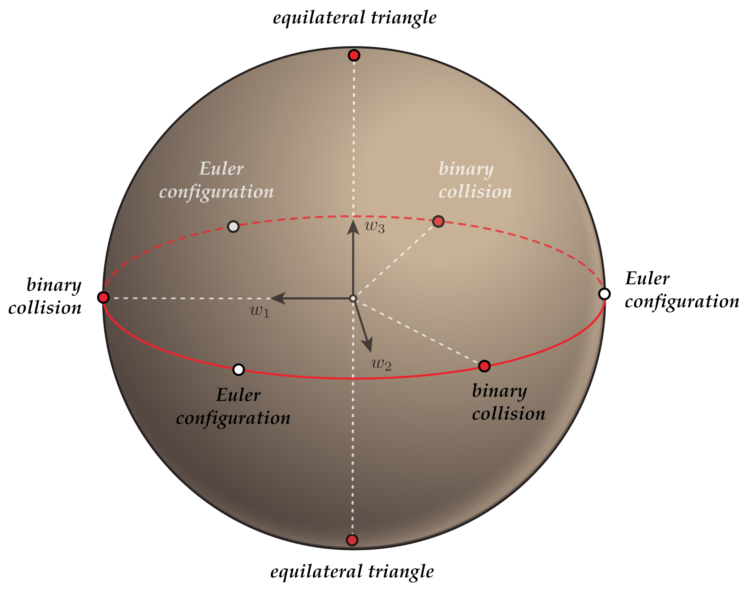
Figure 1.
The shape sphere of the equal-mass 3-body problem. Every point on the sphere(defined as a constant- surface) is a triangle. Points at the same longitude with opposite latitudes correspond to mirror-conjugated triangles. At the poles (the intersections with the axis) we have the equilateral triangles, while on the equator (the red circle, ) we have the collinear configurations. Among them, there are six special ones: three binary collisions (red dots, one of which is on the axis), and Euler configurations (white dots), in which the gravitational force acting on each particle points towards the center of mass and has a magnitude such that, if the system is prepared in rest at one of these configurations, it will fall homothetically (without changing its shape) to a total collision at the centre of mass. The same thing happens at the equilateral triangle (for all values of the masses, as Lagrange showed). Notice that the Euler configurations and binary collisions are on the equator for all values of the three masses, but their relative positions on the equator depends on the masses. The equilateral triangles are at the poles only in the equal-mass case.
The norms of the original Jacobi coordinate vectors can be written as
and, therefore, the full vectors are specified by
where is an overall orientation angle which is not rotation-invariant and, therefore, is not fixed by the specification of the coordinates ; and is the angle between and .
We now want to find the momenta conjugate to . To do so, we consider the symplectic potential
If we replace with their expressions in terms of from Equation (47), we get
where
so we now have a complete canonical transformation from the coordinates (, , ; , , ) to (, , , , ; , , , , ). The Poisson brackets in these coordinates are canonical, as they should be:
In the new coordinates, the kinetic energy decomposes as
and Newton’s potential takes the form
where are the longitudes on the shape sphere of the two-body collisions between particle a and b. These can be found by using Equation (44):
- If , then , and, therefore, , and : we are on the equator and on the axis 1. Moreover , so
- If , then , and, therefore, and we are on the equator. The 1 and 2 coordinates have values and , and so the corresponding longitude is:
- If , the same reasoning above applies to show that we are on the equator, because is parallel to . Then , and , and the longitude is then
If we call the azimuthal and the polar angle on the shape sphere, then
and on the constraint surface the Hamiltonian takes the form
where
is the 3-body “complexity function” (according to the nomenclature used in [8,13,15,16]). Finally, a short calculation reveals that the dilatational momentum takes basically the same form in the new coordinates:
We now want to separate the scale and shape degrees of freedom. Let us use as our scale, and the angles and as our shape coordinates. The symplectic potential now takes the form
where
which can be inverted as
which puts the Hamiltonian in the following form:
where the kinetic term K is a quadratic form in the momenta , and , which is positive definite for any value of and :
In the zero angular momentum case , the equations of motion are:
and in Lagrangian form:
Finally, in the new coordinates the dilatational momentum is of the following form:
3.2. Total Collisions in the Zero-Energy 3-Body Problem
In the previous subsection we described the phase space reduction of the 3-body problem (in the planar case, i.e., orthogonal to the plane of the three bodies) to shape degrees of freedom plus scale (the square root of the moment of inertia). We ended up with a spherical shape space coordinatized by two angles, and , plus a global orientation angle and the scale , as well as their four conjugate momenta , , , and with canonical symplectic structure. If we specialize to the zero angular momentum case (the only case we are interested in if we want to study total collisions), the coordinate drops out of the problem too, because it is cyclic, and we are left with two shape-space coordinates plus one scale, and their conjugate momenta. Conservation of energy is expressed by the following constraint equation:
where E is a constant (the total energy of the system), K is the shape kinetic energy, written in Equation (65), and is what we have been calling (see [8,13,15,16]) the complexity function, as defined in Equation (59). is positive-definite, and we will study the vicinity of one of its stationary points, of coordinates . The equations of motion in Newtonian time for the scale degree of freedom are:
which proves that the dilatational momentum is monotonic. Since D is monotonic, we can use it as an internal time parameter with .
Note that, already at this point, the Hamiltonian constraint, together with the fact that at total collisions (which follows from the Lagrange–Jacobi equation, see above), implies that total collisions can happen only if the angular momentum and the shape momenta are all zero. In fact, multiplying (69) by , we obtain:
which, in the limit and , implies , and K is a positive-definite quadratic form in , , and (65).
As mentioned above, given that is monotonic, we can use it as an internal time parameter. Now the evolution with respect to , in the zero-energy case , is described by the shape Hamiltonian , the canonical conjugate of expressed in terms of the shape variables by means of the Hamiltonian constraint (we obtain a reduced Hamiltonian dynamics on shape space precisely because D, our new internal time parameter, is the dilatational momentum, i.e., the generator of scalings, cf. [8]). To determine , we thus demand , so that is the logarithm of the solution of with respect to r. With replaced by , it is:
It follows that the equations of motion of the “decoupled system” are
We would now like to impose that the system undergoes a total collision. By what we have seen in the previous section, this can only happen at a central configuration (the stationary points of ), and with vanishing dilatational momentum (). However, imposing that the solution goes through a central configuration at the instant is not enough: it could simply be reaching a minimum of the moment of inertia (a Janus point) with the shape of a central configuration, and, past this minimum, grow again without ever hitting a total collision. In order to get an actual total collision, the moment of inertia has to vanish, that is, we need to have that . However, according to Equation (73), r is no longer part of our description of the system (at this level of description, we already are on shape space). The problem is now: if all I have is system (73), how can I tell whether I reached a total collision or simply a Janus point with the shape of a central configuration? Is there a ‘manifest cause’ for a total collision, which can be read off the curve on shape space?
The answer is yes: if some shape momenta and are non-zero at a central configuration, Equation (73) tend to those of a spherical geodesic (in case the central configuration is on the equator of our coordinate system, the term associated to the non-zero Christoffel symbols of the spherical metric on shape space, , vanishes, and the equations reduce to those of a straight line). Otherwise, if both and , Equation (73) appear to diverge. Indeed, it turns out that at a total collision the shape momenta must vanish (compare the remark above). Reconsider the Hamiltonian constraint (69) and multiply it by :
We know, from the discussion of the previous sections, that the dilatational momentum vanishes at a total collision, and, therefore, . Moreover, the complexity function remains bounded, and the quantity E is a constant of motion, so, in the limit , must vanish, which implies and (cf. Reichert [17]). This is a remarkable result in itself, for it tells us that there exists a unique description of total collisions on (scale-free) shape space.
We conclude that, in order to discuss a total collision, we need to focus on those solutions of Equation (73) which are perfectly tuned to reach a central configuration with exactly zero shape momenta. Let us now expand Equation (73) in the vicinity of a central configuration , , and assume for simplicity that our coordinate system places this central configuration on the equator (i.e., ):
where are the components of the Hessian matrix of the logarithm of the complexity function at the central configuration.
Now we can assume that and are small, too, as we want to focus on a total collision which will make them vanish at , so we can write and and expand at first order in :
This last step killed the Christoffel term, and gave us a set of linear equations that can be diagonalized and solved.
3.3. Asymptotics of Total-Collision Solutions
Equation (76) can be diagonalized. Let be the i-th eigenvalue of the Hessian matrix H with components . Then, where is the diagonalized matrix (with eigenvalues as diagonal entries) and T is composed of the normalized eigenvectors. Multiply Equation (76) from the left with T and you obtain:
with
As a system of first-order ODEs, the above clearly does not satisfy the Picard–Lindelöf theorem at : the right-hand side of the first equation is not continuous there, let alone Lipshitz-continuous.
To solve the above equations, multiply the first by and differentiate:
and, replacing the second equation to eliminate :
Now, the solutions of an equation of this form can be looked in the form of a monomial , which, when replaced in the equation, leads to the characteristic polynomial equation:
The above equation admits two solutions: , and, therefore, the general solution of the differential equation is:
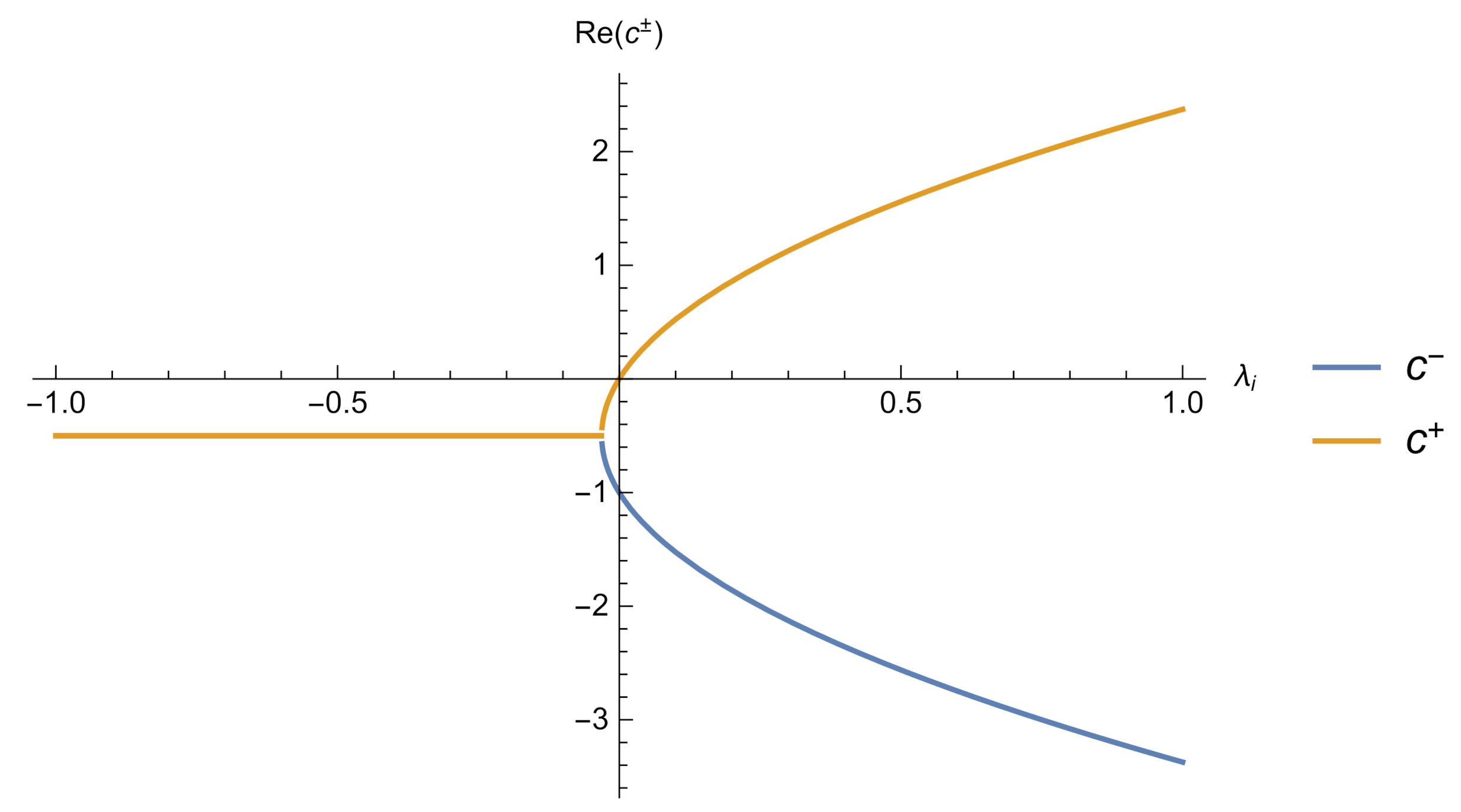
We plot here the real part of vs. (Figure 2):
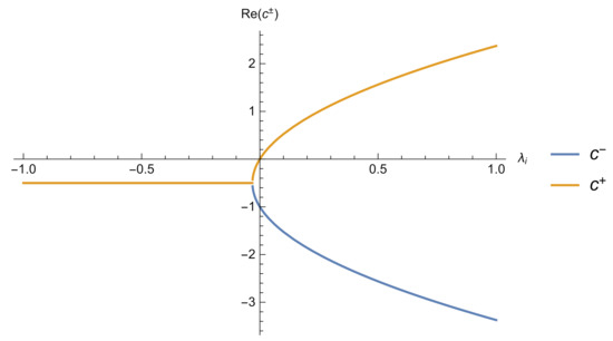
Figure 2.
The real part of and vs. .
We can see how if is negative (as can happen at a saddle point of the shape potential), then the real part of both and is negative. This means that, if we want to impose that the solution converges as , we will have to set for each negative eigenvlue.
If the eigenvalue is positive, then we see from the plot that while for all , so we have to set .
3.4. Generalization to Arbitrary N and Non-Zero Energy
To generalize the result from to arbitrary N, we consider the kinetic metric on the extended configuration space:
this, in terms of the mass-rescaled Jacobi coordinates, becomes
where coordinatize the relative configuration space (the configuration space quotiented by translations).
Now, we can separate the scale and the scale-invariant degrees of freedom by defining the (square root of the) center-of-mass moment of inertia, the scale coordinate:
and the translation-invariant configuration space appears now as the Cartesian product between the scale coordinate and a -dimensional hypersphere which we call pre shape space. (Pre shape space is the quotient of the extended configuration space, , by dilatations and translations alone (keeping the redundance due to rotations)).
To further quotient global rotations out, we need to exploit the fact that they act as an subgroup of the rotation group that realizes the isometries of the -sphere of pre shape space. Quotienting a sphere by a subgroup of its rotation group always results in another sphere. In our case, the end result is a -sphere: shape space. The kinetic metric then decomposes according to an analog formula to Chazy’s kinetic energy decomposition theorem and, in the hyperspherical coordinates on pre-shape space, can be written as
There are conjugate momenta to , , , one conjugate momentum to r, , 3 conjugate momenta to , and 3 components of the total angular momentum . The kinetic energy can then be decomposed as
where is the inverse of the hyperspherical metric, and the Newton potential can be written as
with no dependence on the coordinates of the center of mass, which of course implies that their equations of motion are and their motion can be decoupled from the rest. Assuming now that the angular momentum is zero, and after reabsorbing the kinetic energy of the center of mass into E, the Hamiltonian constraint takes the form
If the total energy E is zero, by replacing , and solving for r, we get a unique solution:
and the corresponding pre-shape space Hamiltonian is:
the structure of the equations is identical to those for the 3-body problem (73). If now we expand to first order around (the coordinates of a central configuration), and , we get:
where is the Hessian matrix. Now, the Hessian can be diagonalized as before, but there are three zero eigenvalues associated to the directions corresponding to global rotations. For these, we have to put the corresponding momenta to zero, because they are equal to the three components of the total angular momentum of the system, and, unless that is zero, the total collision cannot take place. For those three pre-shape space degrees of freedom, therefore, the equations of motion just say that they are constants, and their conjugate momenta are zero. One is then left with effective equations, one for each independent true shape degree of freedom, of the form:
with real constants depending only on the mass ratios .
If the total energy is not zero, one has a quadratic equation to solve for r, but to avoid having to deal with multiple solutions we can exploit the fact that r is small near the total collision, and solve the Hamiltonian constraint perturbatively:
so
The corresponding equations of motion acquire deformation terms which, at first order in and , take the form:
and both deformation terms are irrelevant as , compared to the undeformed one which diverge like .
3.5. The Stratified Manifold of the Total-Collision Solutions
Each central configuration comes with real eigenvalues . Depending on the nature of the central configurations, they may all be positive (if we are at the minimum of —the equilateral triangle in the case—which has been conjectured to be unique for all N), or some of them may be negative (in the case of a saddle point, like the three collinear Euler configurations in the three-body problem).
From Figure 2, we see that each negative eigenvalue corresponds to a pair of exponents , with negative real part, and therefore the corresponding shape degree of freedom cannot hope to converge to its central-configuration value, unless both integration constants and are set to zero. On the other hand, for each positive eigenvalue, the integration constant has to be put to zero in order for the solution to converge.
Let us assume first that, at the central configuration of interest, there are Mdistinct positive ’s and negative ones, and assume also that the positive eigenvalues are ordered from smallest to largest, . Then only M integration constants remain unspecified, and the solutions are of the following form:
The above describe a -parameter family of distinguished solutions, because any two choices of integration constants, and that are related by
describe the same curve in shape space, just parametrized differently. Within this -dimensional manifold, there are special regions corresponding to the cases in which certain integration constants are zero. Let us, in what follows, list all the possible distinct cases.
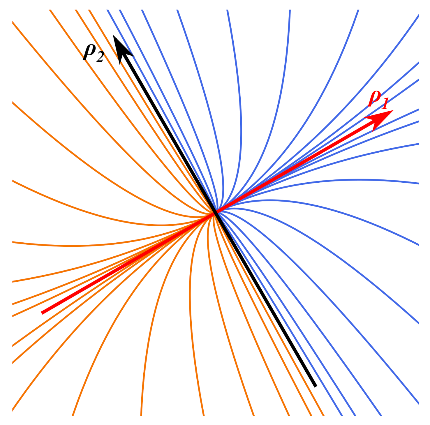
If , then the solution curves all approach the central configuration with the same tangent, parallel to the principal eigendirection (the one corresponding to the largest eigenvalue), and away from it they splay out in all directions, at a pace that is determined by the values of the other integration constants . This is easy to prove: the tangent vector to the parametrized curves is , and normalizing it to one we get a vector that, in the limit , tends to . Moreover, these solutions can be divided in two disjoint components, according to whether is positive or negative. The former approach the central configuration along the positive- axis, the latter along the negative one. In Figure 3, we show an example of this family of solutions for the 3-body problem.
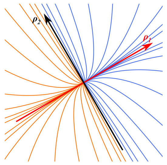
Figure 3.
The total-collision solutions of the 3-body problem, when the asymptotic shape is an equilateral triangle.
- If is zero, but , the solutions lie in the subspace, and the analysis exposed above can be repeated within this subspace, this time with playing the role of principal eigenvalue. The solutions all approach the central configuration tangentially to the axis, and they divide into two connected components, according to the sign of ;
- If , , then the solution lies in the subspace , and the role of principal eigendirection is played by , and the solutions are asymptotically tangent to , and belong to two disconnected components, according to the sign of ;
- If only , then there are only two solutions, which remain always on the positive (respectively negative) axis;
- Finally, if all the are zero, the solution is only the homothetic one, which never changes shape as it falls into a total collision.
What we just described is a stratified manifold of solutions, in which each stratum is obtained from the higher one as the special case in which the first non-zero integration constant of the stratum above is set to zero.
In the case of degenerate eigenspaces (when two or more eigenvalues are identical, which happens for example in the three-body problem when the three masses are equal), the count of free integration constants does not change, and, therefore, the dimension of the space of solution is the same as above, as is its structure as stratified manifold. What changes is the fact that, when the degenerate eigenvalue is the principal one (because it is the smallest, or because the integration constants associated to the eigendirections of smaller eigenvalues have been all put to zero), the solution curve can approach the total collision from any direction within the degenerate eigenspace.
3.6. The Essential Singularity of Total Collisions
In the previous subsection, we have shown how the total-collision solutions can only approach the central configuration along one of the eigendirections of the Hessian matrix that are associated to a positive eigenvalue. Moreover, we have shown that, in the case of distinct eigenvalues, the solutions that approach the total collision from the eigendirection associated to the lowest positive eigenvalue are just two. The ones approaching it from the second-smallest eigendirection are two disjoint one-parameter families; the ones approaching from the third-smallest eigendirection are two disjoint two-parameter families, and so on, all the way to the highest stratum, which consists of two disjoint -parameters families of solutions. The largest possible stratum of solutions for N particles can be obtained in the case in which all eigenvalues are positive, which means that the corresponding central configuration is a minimum of the complexity function. Then, there is a stratum which is (-dimensional. So, for example, in the unequal-mass three-body problem, if the total collision asymptotes to an equilateral triangle (the absolute minimum of the complexity function), we get two one-parameter families of solutions.
We know what the tangent to these solution curves does, but knowing the tangent is not enough to fix all integration constants , while the values of the integration constants determine the solution. Since we are interested in investigating the possibility of continuing each solution in a unique way through the total collision, we want to check whether there exist some variables whose values fix all integration constants, and are well-defined at the total collision. One might look for such ‘manifest causes’ in the geometry of the curve on shape space, which, according to the conjecture at the basis of shape dynamics, captures all there is to know about physical reality. However, one can show that, in the generic case (that is, when none of the constants are commensurable), no differential quantity defined on shape space can fix these integration constants, because at total collisions we have an essentialsingularity. We can see this in this way. Consider the normalized -derivative vector of our solution curve:
As , this quantity asymptotes to
So, imagine we want to join two curves that asymptote to the same central configuration, characterized by integration constants and , one reaching the total collision from below () and one from above (). They both reach the same point at , so whatever pair of curves we choose, they will always be continuous. Now, ask that their tangent is continuous: we want the normalized first derivatives to match. This imposes
that is, the two curves have to approach from the two opposite directions. This can be immediately seen from Figure 3 in the 3-body case. However, if now we hope to fix any further relations between integration constants by asking that any further normalized derivative is continuous, we are disappointed. Once we assume that and have opposite signs, all derivatives are automatically continuous. We could join any two curves in Figure 3, provided they live in opposite sides of the black axis, and they would always be infinitely differentiable. This is a behavior that signals the presence of an essential singularity: for example the function at tends to zero, as do all of its derivatives. This function is not analytic in zero, because it is the inverse of , which is a textbook example of essential singularity (the function and all of its derivatives diverge in zero).
There are exceptions to this result, in the exceptional case in which, due to the particular values of the eigenvalues and , the ratio of the associated constants is a rational number. Then, in this case, there exist integers and , such that the variables and admit the finite ratio at , which allows us to extract some information on the integration constants and at the singularity. Then, if all M positive eigenvalues are such that the corresponding constants are commensurable, we can define a set of M variables, by raising the to appropriate integer powers, that all tend to zero at as the same power of . The simplest such case is that of all-equal eigenvalues, where all converge to zero with the same power law. Then, in this case, all solutions can be continued uniquely at the singularity, and there is a simple change of variables that makes the equations of motion regular there. These cases, however, account for a countable set of choices of masses, and the generic situation is that described above, of an essential singularity preventing continuation.
4. Conclusions
As shown in [8,9], the dynamics of the N-body problem can be equivalently formulated as a non-autonomous system of ODEs on shape space, reducing the system to its irreducible core of physical degrees of freedom. In this formulation, as was shown in [17], the total-collision solutions can be characterized neatly as solutions that end at a central configuration with zero dilatational momentum and zero shape momenta. The question then arises, of whether these solutions can be regularized in the manner of two-body collisions, or continued through the singularity similarly to what was done for cosmological solutions of general relativity in [18,19,20]. Regardless of whether the system has positive or zero energy, the asymptotics of the total-collision solutions is universal, and it is captured by Equation (94), which are completely determined by the eigenvalues of the Hessian matrix of the (log of) the shape potential at the central configuration. If the central configuration is a minimum of the shape potential, these eigenvalues are all positive and one has a manifold of total-collision solutions of maximal dimension (), and for each negative eigenvalue, the dimension of the total collision manifold decreases by one. The manifold has the structure of a stratified manifold, each stratum obtained by considering the integration constant that were non-zero in the stratum above, and setting to zero the one that corresponds to the highest eigenvalue. In each stratum, the solution curves will approach the singularity tangentially to the eigendirection corresponding to the highest eigenvalue whose integration constant is non-zero.
At the singularity, unless one considers very special choices of masses (e.g., all identical), the dynamical system has an essential singularity, which erases (at least some) information regarding all finite-degree derivatives of the dynamical variables, much like the limit of the function, whose derivatives are all zero at the singularity. This mirrors what was found in certain homogeneous-but-non-isotropic cosmological models (namely Bianchi IX), where the system, when studied on shape space (In the case of general relativity, with shape space we mean the space of conformal 3-geometry. Similarly to what happens in the N-body problem, a curve on this shape space codifies all the information that is necessary to reconstruct uniquely a solution of general relativity [9]) behaves like a chaotic billiard ball (what Misner nicknamed “mixmaster behavior”) which bounces an infinite amount of times in any finite proper-time interval ending at the big bang singularity. This, too, is an essential singularity: the limit set of the dynamics is the border of shape space (which has the topology of a circle), but the location on this border does not admit a well-defined limit, much like the value of when (another classic example of essential singularity).
In the case of Bianchi IX, however, there is a simple extension of the model that removes this singularity: adding a scalar field whose potential does not grow too fast for large values of the field [18,19]. The scalar field changes the asymptotics of the shape momenta in such a way that the “mixmaster” chaotic behavior stops after a finite number of bounces, and the system settles on a so-called “quiescent” solution that admits a well-defined limit at the singularity. This is the foundation of the result [18,19] on the continuation of these solutions through the singularity. Interestingly, this regularization could be attributed to quantum effects, because the Starobinski potential satisfies the conditions specified in [19] for the onset of quiescence. In fact, a scalar field with this particular potential emerges as the lowest-order quantum correction to the Einstein–Hilbert action in an effective field theory approach (it is due to an term in the action).
It is possible that the total collisions of the N-body model we studied in the present paper might admit a similar regularization, at the cost of adding some correction terms to the dynamics, which become relevant only near a singularity. This would, however, be a departure from the purely Newtonian N-body problem, and is beyond the scope of the present paper.
Author Contributions
Conceptualization, investigation, and formal analysis, F.M. and P.R.; writing—original draft preparation, F.M.; writing—review and editing, P.R. Both authors have read and agreed to the published version of the manuscript.
Funding
This research received no external funding.
Institutional Review Board Statement
Not applicable.
Informed Consent Statement
Not applicable.
Data Availability Statement
Not applicable.
Acknowledgments
We thank Julian Barbour, Tim Koslowski, and three anonymous referees for valuable comments. F.M. thanks the Action CA18108 QG-MM from the European Cooperation in Science and Technology (COST), the Foundational Questions Institute (FQXi) and the Spanish Ministry of Education.
Conflicts of Interest
The authors declare no conflict of interest.
References
- Sundman, K.F. Recherches sur le problème des trois corps. Acta Soc. Sci. Fenn. 1907, 34, 6. [Google Scholar]
- Sundman, K.F. Mémoire sur le problème de trois corps. Act. Mathemat. 1912, 36, 105–179. [Google Scholar] [CrossRef]
- Siegel, C.L. Singularities of the 3-Body Problem; Tata Institute of Fundamental Research: Bombay, India, 1967. [Google Scholar]
- Simó, C. Masses for which triple collision is regularizable. Celest. Mech. 1980, 21, 25–36. [Google Scholar] [CrossRef]
- Easton, R. Regularization of vector fields by surgery. J. Differ. Equ. 1971, 10, 92–99. [Google Scholar] [CrossRef] [Green Version]
- McGehee, R. Triple Collision in the Collinear Three-Body Problem. Invent. Math. 1974, 27, 191–228. [Google Scholar] [CrossRef]
- Saari, D. Collisions, Rings, and Other Newtonian N-Body Problems; CBMS Regional Conference Series in Mathematics, Number 104; American Mathematical Society: Providence, RI, USA, 2005. [Google Scholar]
- Barbour, J.; Koslowski, T.; Mercati, F. A gravitational origin of the arrows of time. arXiv 2013, arXiv:1310.5167. [Google Scholar]
- Mercati, F. Shape Dynamics: Relativity and Relationalism; Oxford University Press: Oxford, UK, 2018. [Google Scholar] [CrossRef]
- Chazy, J. Sur certaines trajectoires du probléme des n corps. Bull. Astronom. 1918, 35, 321–389. [Google Scholar]
- Saari, D. The manifold structure for collision and for hyperbolic-parabolic orbits in the n-body problem. J. Diff. Equ. 1984, 55, 300–329. [Google Scholar] [CrossRef] [Green Version]
- Lagrange, J.L. Essai sur le problème des trois corps. Oeuvres 1772, 6, 229–324. [Google Scholar]
- Barbour, J.; Koslowski, T.; Mercati, F. Entropy and the Typicality of Universes. arXiv 2015, arXiv:1507.06498. [Google Scholar]
- Montgomery, R. Infinitely Many Syzygies. Arch. Ration. Mech. Anal. 2002, 164, 311–340. [Google Scholar] [CrossRef]
- Barbour, J.; Koslowski, T.; Mercati, F. Identification of a gravitational arrow of time. Phys. Rev. Lett. 2014, 113, 181101. [Google Scholar] [CrossRef] [PubMed] [Green Version]
- Barbour, J.; Koslowski, T.; Mercati, F. Janus Points and Arrows of Time. arXiv 2016, arXiv:1604.03956. [Google Scholar]
- Reichert, P. Investigating total collisions of the Newtonian N-body problem on shape space. Found. Phys. 2021, 51, 32. [Google Scholar] [CrossRef]
- Koslowski, T.; Mercati, F.; Sloan, D. Through the big bang: Continuing Einstein’s equations beyond a cosmological singularity. Phys. Lett. B 2018, 778, 339–343. [Google Scholar] [CrossRef]
- Mercati, F. Through the Big Bang in inflationary cosmology. JCAP 2019, 10, 025. [Google Scholar] [CrossRef] [Green Version]
- Sloan, D. Scalar Fields and the FLRW Singularity. Class. Quant. Grav. 2019, 36, 235004. [Google Scholar] [CrossRef] [Green Version]
Publisher’s Note: MDPI stays neutral with regard to jurisdictional claims in published maps and institutional affiliations. |
© 2021 by the authors. Licensee MDPI, Basel, Switzerland. This article is an open access article distributed under the terms and conditions of the Creative Commons Attribution (CC BY) license (https://creativecommons.org/licenses/by/4.0/).