Symmetry in Neutrino Oscillation in Matter: New Picture and the νSM–Non-Unitarity Interplay

Abstract

We update and summarize the present status of our understanding of the reparametrization symmetry with an $i\leftrightarrow j$ state exchange in neutrino oscillation in matter. We introduce a systematic method called “Symmetry Finder” (SF) to uncover such symmetries, demonstrate its efficient hunting capability, and examine their characteristic features. Apparently they have a local nature: the 1–2 and 1–3 state exchange symmetries exist at around the solar and atmospheric resonances, respectively, with the level-crossing states exchanged. However, this view is not supported, to date, in the globally valid Denton et al. (DMP) perturbation theory, which possesses the 1–2, but not the 1–3, exchange symmetry. This is probably due to our lack of understanding, and we find a clue for a larger symmetry structure than we know of. In the latter part of this article, we introduce non-unitarity, or unitarity violation (UV), into the $\nu$SM neutrino paradigm, a low-energy description of beyond $\nu$SM new physics at a high (or low) scale. Based on the analyses of UV extended versions of the atmospheric resonance and the DMP perturbation theories, we argue that the reparametrization symmetry has a diagnostic capability for the theory with the $\nu$SM and UV sectors. Speculation is given on the topological nature of the identity, which determines the transformation property of the UV $\alpha$ parameters.

1. Introduction

Symmetry is one of the deepest subjects in physics. When one picks up a field theory textbook from bookshelf, say, ref. [1], one finds the description of various symmetries, space-time symmetries, internal symmetries, $CP$, T, and $CPT$, discrete symmetries, symmetry in the hadron spectrum, and $O\left(4\right)$ in the Coulomb problem, not to mention gauge symmetry for constructing the Standard Model (SM). Most likely, even the several big monographs would not be sufficient for full coverage of the subjects because of its profound consequences and evolving nature. Fortunately, a set of beautiful lectures on symmetry in particle physics delivered in the last decades in the 20th century is left for us [2].

In this paper, we discuss the reparametrization symmetry in neutrino oscillation in matter. It indeed has quite different character from those described in refs. [1,2]. Invariance under reparametrization merely implies that there is another way of parametrizing the equivalent solution of the theory. Consequently, a general view on such symmetry would be that it might be useful, but no conceptually deep notion is likely to be involved. Recently, however, we have been accumulating new experiences about the reparametrization symmetry [3,4,5], which may introduce a new perspective on this view. Therefore, in this paper, we present our self-contained global picture of the symmetry in neutrino oscillation in matter with the hope of bringing the subject to the readers’ attention and for a new judgement. If successful, we could possibly overturn the above prejudice about reparametrization symmetry.

What does symmetry look like in neutrino oscillation in matter? Let us give a simple and concrete example. In a perturbative framework valid at around the atmospheric resonance [6], which will be dubbed as the “helio-perturbation theory” in this paper, it is noticed [7] that the expression of the oscillation probability is invariant under the transformations

$$\begin{array}{ccc}& & {\lambda }_1\leftrightarrow {\lambda }_3,cos\varphi \to \mp sin\varphi ,sin\varphi \to \pm cos\varphi .\hfill \end{array}$$

(1)

The notations are such that $\varphi$ is the ${\theta }_{13}$ in matter, and ${\lambda }_1>{\lambda }_3$ denote the two eigenvalues which participate in the level crossing at around the atmospheric resonance in the inverted mass ordering [6]; see Section 6.2. (In normal mass ordering, ${\lambda }_3>{\lambda }_2$ are the two eigenvalues which have the level crossing [6].) A similar symmetry as in Equation (1) but replacing the 1–3 exchange by the 1–2 exchange using $\psi$ as the matter-dressed ${\theta }_{12}$ (${\theta }_{12}$ in matter) was observed earlier in the Denton et al. (DMP) perturbation theory [8]. The precise meaning of the term “matter-dressed ${\theta }_{12}$” is explained after Equation (19), and similarly for ${\theta }_{13}$ in matter by Equation (44).

Recently, we have developed a systematic method of finding the reparametrization symmetry in neutrino oscillation in matter, termed “Symmetry Finder” (SF) [3,4,5]. We will review this machinery and its powerfulness and try to show the readers where we are in our journey of uncovering and understanding this symmetry. It is interesting in its own right, serving, for example, to keep the consistency of the calculations of the observables, a “bread and butter” item but an important task for the theorists. Eventually, we are going to suggest, in the active three neutrino framework extended to include unitarity violation (UV) that the reparametrization symmetry distinguishes between the $\nu$SM (neutrino-mass-embedded SM) and the UV sectors of the theory, offering a useful tool for diagnosing such theories [5]. We are aware that in the physics literature, UV usually means “ultraviolet”. However, in this paper, UV is used as an abbreviation for “unitarity violation” or “unitarity violating”. We hope that SF, a systematic approach, provides an efficient digging-out machinery for the symmetries in neutrino oscillation in matter and their deeper understanding. We believe that it follows the spirit of the early analyses on symmetries and strengthens their impacts [9,10,11,12,13,14,15,16,17,18].

1.1. Local Character of the Reparametrization Symmetry

To our current understanding, the reparametrization symmetry of neutrino oscillation takes different forms depending upon where we are, i.e., which regions of neutrino energy E, baseline L, and the matter density $\rho$ are along the neutrino trajectory in the kinematical phase space. Therefore, let us first introduce the matter effect [19] and draw a global picture of neutrino oscillation in the earth matter environment. The matter potential will be defined in Equation (13) in Section 3.1. In Figure 1, the equi-probability contour of $P({\nu }_{\mu }\to {\nu }_e)$ is presented [20] in the region of the energy baseline that roughly covers Super-Kamiokande’s atmospheric neutrino observation 0.1 GeV $\lesssim E\lesssim 10$ GeV; see Figure 3 in ref. [21]. It also overlaps with the regions for all the ongoing and planned long-baseline accelerator neutrino experiments. Two peaks are visible: the solar scale ($E\sim 200$ MeV, $L\sim 2000$ km) and the atmospheric scale ($E\sim 8$ GeV, $L\sim {10}^4$ km) enhanced oscillations. For brevity, we refer to these respective regions as the solar resonance and the atmospheric resonance regions hereafter. In this article, the term “resonance” should be understood in this less strict sense than usual; see refs. [19,22,23,24].

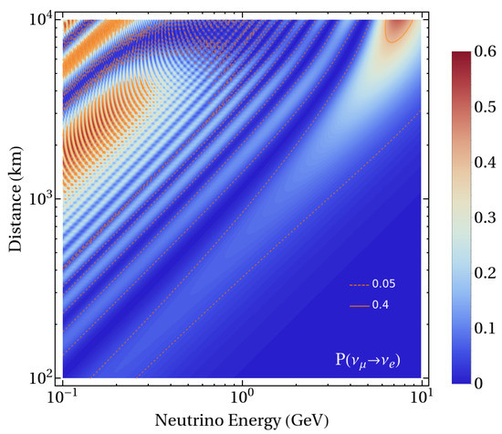
Figure 1. The equi-probability contour of $P({\nu }_{\mu }\to {\nu }_e)$ is presented [20] in region of energy-baseline that covers the atmospheric neutrino observation by Super-Kamiokande. Two peaks are visible: the solar scale ($E\sim 200$ MeV, $L\sim 2000$ km) and the atmospheric scale ($E\sim 8$ GeV, $L\sim {10}^4$ km) enhanced oscillations. The matter density is taken to be a constant, $\rho =4.0{\mathrm{g}/\mathrm{cm}}^3$, which gives only a bold approximation to the Earth matter density.

Now, what we are telling the readers is that the reparametrization symmetry takes different form around each peak. That is,

• In the solar resonance region, the reparametrization symmetry of the 1–2 state exchange type exists, to be discussed in Section 4;
• In the atmospheric resonance region, the reparametrization symmetry of the 1–3 state exchange type exists [4].

Since the symmetry in the framework with local validity in the solar resonance region [7] has never been investigated in the literature, we will fill the gap in this article.

In fact, the features described in the above-itemized statements appeal to our intuition. The 1–2 and 1–3 state level crossings, respectively, are the key to the solar-scale and the atmospheric-scale resonances, and they are the dominant players in these respective regions. The symmetry type specified by the exchanged states mentioned above just reflects the main players in each region; see, e.g., refs. [25,26,27,28] for the earlier versions of the atmospheric resonance perturbation theory. Given the existence of the various versions, not to trigger any confusion, we discuss in this paper the particular version in ref. [6] under the name of “helio-perturbation theory” to discuss the reparametrization symmetry in the atmospheric resonance region. The term “helio-perturbation”, shorthand of the “helio-terrestrial-ratio perturbation”, is invented because it perturbs the dominant effect of the atmospheric resonance by the small solar-scale effect of order $\sim \mathsf{\Delta }{m}_{21}^2/\mathsf{\Delta }{m}_{31}^2\approx 0.03$.

1.2. Globally Valid vs. Locally Valid Frameworks

However, it turned out that the things are not so simple. Progress in the perturbative treatment of neutrino oscillations in matter now allows us to have a limited number of “globally valid” frameworks, the DMP [8] and Agarwalla et al. (AKT) [29] theories. By “globally valid”, we mean that the framework is valid throughout the terrestrial region depicted in Figure 1. In fact, the region of validity of the globally valid frameworks is likely to extend to much higher energies, which is explored, e.g., by IceCube-DeepCore [30]. See the related discussions in ref. [31]. As opposed to the above-mentioned “locally valid” theories, a globally valid theory is able to describe the both solar and atmospheric resonances. The secret for such greater capability is in the usage of the Jacobi method; see ref. [29] for a concise exposition of the Jacobi method.

Does the globally valid framework allow us to formulate the reparametrization symmetry in both the solar and atmospheric resonance regions? Thus far, the answer is no. According to the result of ref. [3], only the reparametrization symmetry of the 1–2 state exchange type is obtained, or, in other words, the better way of formulating SF such that the potential of the globally valid frameworks is fully utilized remains to be discovered. Remember, however, that the problem has been examined only in the DMP theory so far, and it is interesting to know how the problem looks like in the AKT perturbation theory [29]. While the present author is suspicious about the above conclusion, it is the current status of our understanding of the reparametrization symmetry in neutrino oscillation in matter. In close relationship to this point, a conjecture is given toward the generalization of the SF formalism to accommodate much more generic reparametrization symmetry [5].

Here are additional (not so pedagogical) comments on the globally valid vs. locally valid frameworks of neutrino oscillation. One may argue that the wider coverage indicates the superiority of the globally valid framework over the local frameworks. Moreover, one can show that the DMP preserves the Naumov identity [32], at least approximately [4]. This is a necessary condition that has to be satisfied for the globally valid framework, while the helio-perturbation theory does not support this property for a good reason [4]. Nonetheless, we would like to emphasize that it is only one side of the coin. From the viewpoint of our symmetry discussion, a one-to-one correspondence between the crossing of the resonant level and the existing symmetry type is revealing and looks physically appealing.

1.3. Paper Plan: Part I and II

This paper has the two parts. Part I spans from Section 1, Section 2, Section 3 and Section 4, and Part II spans from Section 5, Section 6, Section 7, Section 8 and Section 9. In Part I, we define the target of our discussion, the reparametrization symmetry of the state exchange type, and introduce the concept of “Symmetry Finder” (SF), a systematic way of hunting the reparametrization symmetry; see Section 2. We briefly describe the 1–2 state exchange symmetry in the DMP perturbation theory [3] as a prototype of such symmetry we discuss in this article. In Section 3, we review the solar resonance perturbation (SRP) theory [7] and introduce the V matrix method [33]. In Section 4, we formulate SF for the SRP theory and analyze the SF equation to obtain the 1–2 exchange symmetry. The SF treatment of the SRP theory has not been done before, so we are going to add something new in this subject. Our discussion will be pedagogical in most part of Part I, aiming at facilitating the readers’ understanding of the subject. For this purpose, we restrict ourselves to $\nu$SM symmetry in Part I.

In Part II, we focus on the reparametrization symmetry in the theory with the non-unitary flavor mixing matrix, or UV; see refs. [34,35,36,37,38], for example, with more references coming later. As overviewed in Section 5, looking for new physics beyond the $\nu$SM is a vigorously pursued subject in particle physics, and non-unitarity is one of the promising ways for its low-energy description. We are interested in such a possibility that the symmetry can be used as a diagnostics tool for the theory with the $\nu$SM and UV sectors. For this purpose, we feel, non-unitarity would provide a useful testing ground for such a possibility because its principle and the relation to the high- or low-energy new physics is relatively well defined [34,35,36,37,38]. In Section 6, Section 7, Section 8 and Section 9, we give a self-contained treatment of the 1–3 state exchange symmetry in the helio-UV perturbation theory [39], a UV extension of the helio-perturbation theory [6]. Since the SF treatment of the helio-UV perturbation theory has never been done in the literature, the derivation and discussion of such symmetry in this theory is all new.

In summary, our goals and the motivating force in this paper are:

• Part I: We summarize the current status of our understanding of the reparametrization symmetry of the state exchange type in neutrino oscillation in matter. To the best of our knowledge, no one expected that so many symmetries are hidden in the DMP and the helio-perturbation theories [3,4]. A tantalizing question is: what are the nature and implications of the symmetry?
• Part II: We introduce non-unitarity and analyze the symmetry in the UV-extended frameworks of neutrino evolution. We realize the possible utility of the symmetry as a diagnostics tool for theories with the $\nu$SM and UV sectors. A part of the reparametrization symmetry acts only on the $\nu$SM variables, not UV ones, distinguishing between the two sectors of the theory [5]. Can we observe the whole picture of this?

2. Introducing Symmetry Finder

Is there a systematic way of uncovering reparametrization symmetry in neutrino oscillation? Our answer is yes: Symmetry Finder (SF) does the job in a vacuum [40] and in matter [3,4,5]”.

Let us consider that the expression of the flavor basis state (i.e., wave function) $\nu$ in terms of the mass eigenstate $\overline{\nu }$ in a vacuum or in matter in the following two different ways,

$$\begin{array}{ccc}& & \nu =U({\theta }_{23},{\theta }_{13},{\theta }_{12},\delta )\overline{\nu }=U({\theta }_{23}^{\prime },{\theta }_{13}^{\prime },{\theta }_{12}^{\prime },{\delta }^{\prime }){\overline{\nu }}^{\prime },\hfill \end{array}$$

(2)

where the quantities with “prime” imply the transformed ones, and ${\overline{\nu }}^{\prime }$ may involve eigenstate exchanges and/or rephasing of the wave functions. If it is in matter, the mixing angles and the CP phase can be elevated to the matter-dressed variables. Since the SF equation represents the same flavor state by the two different sets of the physical parameters, it implies symmetry.

2.1. The PDG and SOL Conventions of the Flavor Mixing Matrix

To discuss the 1–2 state exchange symmetries in a vacuum and in matter, which we will do in Part I, it is convenient to introduce the flavor mixing matrix $U\equiv U_{\mathrm{MNS}}$ [41] in a convention called “SOL” [39,40], which is slightly different from the usual particle data group (PDG) convention [42],

$$\begin{array}{c}{U}_{\mathrm{SOL}}\equiv \left[\begin{array}{ccc}1& 0& 0\\ 0& e^{-i\delta }& 0\\ 0& 0& e^{-i\delta }\end{array}\right]U_{\mathrm{PDG}}\left[\begin{array}{ccc}1& 0& 0\\ 0& e^{i\delta }& 0\\ 0& 0& e^{i\delta }\end{array}\right]=\left[\begin{array}{ccc}1& 0& 0\\ 0& c_{23}& s_{23}\\ 0& -s_{23}& c_{23}\end{array}\right]\left[\begin{array}{ccc}{c}_{13}& 0& s_{13}\\ 0& 1& 0\\ -s_{13}& 0& c_{13}\end{array}\right]\left[\begin{array}{ccc}{c}_{12}& s_{12}{e}^{i\delta }& 0\\ -s_{12}{e}^{-i\delta }& c_{12}& 0\\ 0& 0& 1\end{array}\right]\hfill \\ \equiv U_{23}\left({\theta }_{23}\right)U_{13}\left({\theta }_{13}\right)U_{12}({\theta }_{12},\delta ).\hfill \end{array}$$

(3)

In this paper, hereafter, we use the abbreviated notations $c_{ij}\equiv cos{\theta }_{ij}$, $s_{ij}\equiv sin{\theta }_{ij}$, etc., where $ij=12,13,23$. In Equation (3), $\delta$ denotes the lepton analogue of the quark Kobayashi–Maskawa (KM) CP-violating phase [43], and the second line defines the notations for the three rotation matrices in the SOL convention. $U_{\mathrm{PDG}}$ denotes the U matrix in the PDG convention [42]

$$\begin{array}{ccc}\hfill U_{\mathrm{PDG}}& =& \left[\begin{array}{ccc}1& 0& 0\\ 0& c_{23}& s_{23}\\ 0& -s_{23}& c_{23}\end{array}\right]\left[\begin{array}{ccc}{c}_{13}& 0& s_{13}{e}^{-i\delta }\\ 0& 1& 0\\ -s_{13}{e}^{i\delta }& 0& c_{13}\end{array}\right]\left[\begin{array}{ccc}{c}_{12}& s_{12}& 0\\ -s_{12}& c_{12}& 0\\ 0& 0& 1\end{array}\right]\hfill \\ & \equiv & U_{23}\left({\theta }_{23}\right)U_{13}({\theta }_{13},\delta )U_{12}\left({\theta }_{12}\right),\hfill \end{array}$$

(4)

with the second line being the rotation matrices in the PDG convention. The reason for our terminology of $U_{\mathrm{SOL}}$ in Equation (3) is because the CP phase factor $e^{\pm i\delta }$ is attached to (the sine of) the “solar angle” ${\theta }_{12}$ in $U_{\mathrm{SOL}}$, whereas in $U_{\mathrm{PDG}}$, $e^{\pm i\delta }$ is attached to $s_{13}$. Notice that the convention change from the PDG to SOL conventions does not alter the oscillation probability because the rephasing factors in Equation (3) can be absorbed into the neutrino wave functions, leaving no effect in the observables. In Part II, we will use the PDG convention for convenience to treat the 1–3 exchange symmetry in the helio-perturbation theory [4] and its UV extension.

2.2. Symmetry Finder (SF) in Vacuum

The idea of SF has a simple realization in a vacuum where the flavor eigenstate $\nu$ is related to the mass eigenstate $\overline{\nu }$ using the SOL convention U matrix (3)

$$\begin{array}{ccc}& & \nu =U\overline{\nu }=U_{23}\left({\theta }_{23}\right)U_{13}\left({\theta }_{13}\right)U_{12}({\theta }_{12},\delta )\overline{\nu }.\hfill \end{array}$$

(5)

Then, one can easily prove the relation

$$\begin{array}{ccc}& & U_{12}({\theta }_{12},\delta )\left[\begin{array}{c}{\nu }_1\\ {\nu }_2\\ {\nu }_3\end{array}\right]=U_{12}\left({\theta }_{12}+\frac{\pi }{2},\delta \right)\left[\begin{array}{c}-e^{i\delta }{\nu }_2\\ e^{-i\delta }{\nu }_1\\ {\nu }_3\end{array}\right]=U_{12}\left(\frac{\pi }{2}-{\theta }_{12},\delta \pm \pi \right)\left[\begin{array}{c}{e}^{i\delta }{\nu }_2\\ -e^{-i\delta }{\nu }_1\\ {\nu }_3\end{array}\right].\hfill \end{array}$$

(6)

Hereafter, the state ${\nu }_1$ denotes the one with the largest ${\nu }_e$ component. The state ${\nu }_2$ is the one that is separated from the state ${\nu }_1$ by the mass squared difference

$m_2^2-m_1^2\equiv \mathsf{\Delta }{m}_{\mathrm{solar}}^2\simeq 7.5\times {10}^{-5}$ eV² > 0.

As we stated above, the relation (6) implies symmetry [40]. The first equality means that the use of ${\theta }_{12}^{\prime }={\theta }_{12}+\frac{\pi }{2}$ and the exchanged (and rephased) mass eigenstates $1\leftrightarrow 2$ produces the same oscillation probability. Since rephasing does not affect the observables, the first equality in Equation (6) implies 1–2 exchange symmetry under the transformation

$$\begin{array}{ccc}& & \mathrm{Symmetry}\mathrm{IA}\text{-}\mathrm{vacuum}:m_1^2\leftrightarrow m_2^2,c_{12}\to -s_{12},s_{12}\to c_{12}.\hfill \end{array}$$

(7)

The existence of an alternative choice, $c_{12}\to s_{12}$ and $s_{12}\to -c_{12}$ (${\theta }_{12}\to {\theta }_{12}-\frac{\pi }{2}$), should be understood. Similarly, the second equality in (6) implies the symmetry of the probability under the transformation

$$\begin{array}{ccc}& & \mathrm{Symmetry}\mathrm{IB}\text{-}\mathrm{vacuum}:m_1^2\leftrightarrow m_2^2,c_{12}\leftrightarrow s_{12},\delta \to \delta \pm \pi .\hfill \end{array}$$

(8)

2.3. Symmetry Finder in Matter

In the exact diagonalization scheme of Zaglauer and Schwarzer (ZS) [44], the Hamiltonian is formally identical to that in a vacuum apart from the replacements of the mixing angles ${\theta }_{ij}$ to the matter-dressed ones ${\tilde{\theta }}_{ij}$, $\delta \to \tilde{\delta }$, and the eigenvalues $m_i^2\to {\lambda }_i$ ($i,j=1,2,3$). Therefore, the symmetries (7) and (8) are easily elevated to Symmetry IA-ZS and IB-ZS with the fully matter-dressed variables [3,40].

Let us move into the more manageable approximate frameworks. Within the $\nu$SM, so far, the following two types of the reparametrization symmetry are identified and analyzed.

• Eight reparametrization symmetries of the 1–2 state exchange type in DMP [3].
• Sixteen reparametrization symmetries of the 1–3 state exchange type in the helio-perturbation theory [4].

The list will be enriched after Section 4 below by

• Eight reparametrization symmetries of the 1–2 state exchange type in the solar resonance perturbation (SRP) theory.

Notice that the obtained symmetries are so numerous, including the ZS symmetries above, that they cannot occur by accident. A certain nontrivial structure must be behind the appearance of so many symmetries. This then suggests that the existence of the reparametrization symmetry is universal in neutrino oscillation in matter. We shall introduce the various symmetries that appear in several different theories in a step-by-step manner and try to understand their structure in this article.

2.4. Reparametrization Symmetry in DMP

To formulate SF in matter, we need the expression of the flavor basis state $\nu$ in terms of the mass eigenstate $\overline{\nu }$ analogous to Equation (5) in a vacuum. This can be computed with the V matrix method [33], which will be explained in Section 3.4 for the SRP theory. Here, we simply want to show the “atmosphere” of how SF works to find symmetry in matter. Hence, we quote the expression of the flavor basis state in terms of the mass eigenstate to the first order in the DMP perturbation theory computed in ref. [3]:

$$\begin{array}{ccc}\hfill \left[\begin{array}{c}{\nu }_e\\ {\nu }_{\mu }\\ {\nu }_{\tau }\end{array}\right]& =& U_{23}\left({\theta }_{23}\right)U_{13}\left(\varphi \right)U_{12}(\psi ,\delta )\hfill \\ & \times & \left\{1+ϵc_{12}{s}_{12}sin(\varphi -{\theta }_{13})\left[\begin{array}{ccc}0& 0& -s_{\psi }\frac{\mathsf{\Delta }{m}_{\mathrm{ren}}^2}{{\lambda }_3-{\lambda }_1}\\ 0& 0& c_{\psi }{e}^{-i\delta }\frac{\mathsf{\Delta }{m}_{\mathrm{ren}}^2}{{\lambda }_3-{\lambda }_2}\\ s_{\psi }\frac{\mathsf{\Delta }{m}_{\mathrm{ren}}^2}{{\lambda }_3-{\lambda }_1}& -c_{\psi }{e}^{i\delta }\frac{\mathsf{\Delta }{m}_{\mathrm{ren}}^2}{{\lambda }_3-{\lambda }_2}& 0\end{array}\right]\right\}\left[\begin{array}{c}{\nu }_1\\ {\nu }_2\\ {\nu }_3\end{array}\right],\hfill \end{array}$$

(9)

where $\psi$ and $\varphi$ denote, respectively, ${\theta }_{12}$ and ${\theta }_{13}$ in matter. $c_{\psi }$ and $s_{\psi }$ are shorthand notations for $cos\psi$ and $sin\psi$, respectively. $ϵ$ is the unique expansion parameter in the DMP perturbation theory and is defined as

$$\begin{array}{ccc}& & ϵ\equiv \frac{\mathsf{\Delta }{m}_{21}^2}{\mathsf{\Delta }{m}_{\mathrm{ren}}^2},\mathsf{\Delta }{m}_{\mathrm{ren}}^2\equiv \mathsf{\Delta }{m}_{31}^2-s_{12}^2\mathsf{\Delta }{m}_{21}^2,\hfill \end{array}$$

(10)

where $\mathsf{\Delta }{m}_{\mathrm{ren}}^2$ is the “renormalized” atmospheric $\mathsf{\Delta }{m}^2$ used in ref. [6]. The same quantity is known as the effective $\mathsf{\Delta }{m}_{\mathrm{ee}}^2$ in the ${\nu }_e\to {\nu }_e$ channel in vacuum [45]. While we prefer the usage of $\mathsf{\Delta }{m}_{\mathrm{ren}}^2$ in the context of the present paper, the question of which symbol should be appropriate to use here is under debate [6]. The authors of ref. [46] make the choice alternative to ours.

With Equation (9), we write down the equation similar to Equation (6) in a vacuum. The added first-order structure in Equation (9) leads to a proliferation of the reparametrization symmetries, the eight DMP symmetries [3], as tabulated in Table 1. To see how the SF equation is actually formulated and solved, please wait until Section 4.1 and Section 4.2, in which the SRP theory is treated.

Table 1. Summary of the reparametrization symmetries of the 1–2 state exchange type in the DMP and DMP-UV perturbation theories. The column “Type” shows the symmetry type. For the $\nu$SM DMP, look at the first three columns only: the symmetry denoted as “X” in the Type column is referred to as “Symmetry X-DMP” in the text. For the DMP-UV perturbation theory, the fourth column must be included in addition to the first three columns to show the $\tilde{\alpha }$ parameters’ transformation, and the symmetry is denoted as “Symmetry X-DMP-UV”.

Type	Vacuum Parameter Transf.	Matter Parameter Transf.	UV Parameter Transf.
IA	none	${\lambda }_1\leftrightarrow {\lambda }_2$, $c_{\psi }\to \mp s_{\psi }$, $s_{\psi }\to \pm c_{\psi }$	none
IB	${\theta }_{12}\to -{\theta }_{12}$, $\delta \to \delta +\pi$.	${\lambda }_1\leftrightarrow {\lambda }_2$, $c_{\psi }\to \pm s_{\psi }$, $s_{\psi }\to \pm c_{\psi }$	none
IIA	${\theta }_{23}\to -{\theta }_{23}$, ${\theta }_{12}\to -{\theta }_{12}$.	${\lambda }_1\leftrightarrow {\lambda }_2$, $c_{\psi }\to \pm s_{\psi }$, $s_{\psi }\to \pm c_{\psi }$	${\tilde{\alpha }}_{\mu e}\to -{\tilde{\alpha }}_{\mu e}$, ${\tilde{\alpha }}_{\tau \mu }\to -{\tilde{\alpha }}_{\tau \mu }$
IIB	${\theta }_{23}\to -{\theta }_{23}$, $\delta \to \delta +\pi$.	${\lambda }_1\leftrightarrow {\lambda }_2$, $c_{\psi }\to \mp s_{\psi }$, $s_{\psi }\to \pm c_{\psi }$	same as IIA
IIIA	${\theta }_{13}\to -{\theta }_{13}$, ${\theta }_{12}\to -{\theta }_{12}$.	${\lambda }_1\leftrightarrow {\lambda }_2$, $\varphi \to -\varphi$	${\tilde{\alpha }}_{\mu e}\to -{\tilde{\alpha }}_{\mu e}$, ${\tilde{\alpha }}_{\tau e}\to -{\tilde{\alpha }}_{\tau e}$
		$c_{\psi }\to \pm s_{\psi }$, $s_{\psi }\to \pm c_{\psi }$
IIIB	${\theta }_{13}\to -{\theta }_{13}$, $\delta \to \delta +\pi$.	${\lambda }_1\leftrightarrow {\lambda }_2$, $\varphi \to -\varphi$	same as IIIA
		$c_{\psi }\to \mp s_{\psi }$, $s_{\psi }\to \pm c_{\psi }$
IVA	${\theta }_{23}\to -{\theta }_{23}$, ${\theta }_{13}\to -{\theta }_{13}$.	${\lambda }_1\leftrightarrow {\lambda }_2$, $\varphi \to -\varphi$	${\tilde{\alpha }}_{\tau e}\to -{\tilde{\alpha }}_{\tau e}$, ${\tilde{\alpha }}_{\tau \mu }\to -{\tilde{\alpha }}_{\tau \mu }$
		$c_{\psi }\to \mp s_{\psi }$, $s_{\psi }\to \pm c_{\psi }$
IVB	${\theta }_{23}\to -{\theta }_{23}$, ${\theta }_{13}\to -{\theta }_{13}$,	${\lambda }_1\leftrightarrow {\lambda }_2$, $\varphi \to -\varphi$	same as IVA
	${\theta }_{12}\to -{\theta }_{12}$, $\delta \to \delta +\pi$.	$c_{\psi }\to \pm s_{\psi }$, $s_{\psi }\to \pm c_{\psi }$

Table 1 must be used with care. Here, we must focus on the first three columns of Table 1, in which the informations of the $\nu$SM DMP symmetry are tabulated [3]. The fourth column is added to display the $\tilde{\alpha }$ parameter transformation property for the DMP-UV perturbation theory [5], a UV-extended version of the DMP theory [31] to be discussed later. The $\alpha$ parametrization [35] will be used to describe the non-unitary mixing matrix, as defined in Equation (37) in Section 6.1, and $\tilde{\alpha }$ denotes the $\alpha$ parameters in the SOL convention. For the definition of $\tilde{\alpha }$, see Equation (A3) in Appendix A. The fourth column will be useful for a comparison with the case of the UV extended helio-perturbation theory, which will be discussed in Section 7 and Section 8.

Readers may be anxious to know how Table 1 is obtained. If it is a burning question for a reader, he/she can turn to ref. [3] to reproduce the results in the first three columns or ref. [5] for all the four columns. However, instead, we move on to the SRP theory to see the new symmetry results, where we meet a very similar structure to DMP. As our intuition told us in Section 1, the theory will have the symmetries of the 1–2 state exchange type.

3. Solar Resonance Perturbation Theory

The solar resonance perturbation (SRP) theory [7], one of the locally valid theories, aims at describing physics around the solar-scale resonance. In this section, we briefly review the SRP theory toward investigation of the reparametrization symmetry in the theory.

3.1. Three Active-Neutrino System with Unitary Flavor Mixing Matrix

We start by defining the standard three neutrino evolution system in matter. It is defined by the Schrödinger equation in the vacuum mass eigenstate basis, the “check basis”,

$$\begin{array}{c}\hfill i\frac{d}{dx}\check{\nu }=\frac{1}{2E}\left\{\left[\begin{array}{ccc}0& 0& 0\\ 0& \mathsf{\Delta }{m}_{21}^2& 0\\ 0& 0& \mathsf{\Delta }{m}_{31}^2\end{array}\right]+U^{†}\left[\begin{array}{ccc}a-b& 0& 0\\ 0& -b& 0\\ 0& 0& -b\end{array}\right]U\right\}\check{\nu }\equiv \check{H}\check{\nu }.\end{array}$$

(11)

In Equation (11), which defines the check basis Hamiltonian $\check{H}$, U denotes the $3\times 3$ unitary flavor mixing matrix, which relates the flavor basis neutrino state $\nu$ to the vacuum mass eigenstates as

$$\begin{array}{c}\hfill {\nu }_{\alpha }=U_{\alpha i}{\check{\nu }}_i.\end{array}$$

(12)

Hereafter, the subscript Greek indices $\alpha$, $\beta$, or $\gamma$ run over $e,\mu ,\tau$, and the Latin indices i, j run over the mass eigenstate indices $1,2,$ and 3. E is the neutrino energy, and $\mathsf{\Delta }{m}_{ji}^2\equiv m_j^2-m_i^2$. The usual phase redefinition of neutrino wave function is carried out to leave only the mass squared differences. Notice, however, that doing or undoing this phase redefinition does not affect our symmetry discussion in this article.

The functions $a\left(x\right)$ and $b\left(x\right)$ in Equation (11) denote the Wolfenstein matter potentials [19] due to charged current (CC) and neutral current (NC) reactions, respectively,

$$\begin{array}{ccc}\hfill a\left(x\right)& =& 2\sqrt{2}{G}_F{N}_{e}E\approx 1.52\times {10}^{-4}\left(\frac{Y_e\rho }{\mathrm{g}{\mathrm{cm}}^{-3}}\right)\left(\frac{E}{\mathrm{GeV}}\right){\mathrm{eV}}^2,\hfill \\ \hfill b\left(x\right)& =& \sqrt{2}{G}_F{N}_{n}E=\frac{1}{2}\left(\frac{N_n}{N_e}\right)a,\hfill \end{array}$$

(13)

where $G_F$ is the Fermi constant. $N_e$ and $N_n$ are the electron and neutron number densities in matter. $\rho$ and $Y_e$ denote, respectively, the matter density and number of electrons per nucleon in matter. These quantities, except for $G_F$, are, in principle, position dependent. Until reaching Section 9, however, we take the uniform matter density approximation.

In the $\nu$SM unitary three-neutrino system, the NC potential $b\left(x\right)$ does not affect the neutrino flavor change, because it comes as the unit matrix in flavor space. However, it is included in Equation (11) for use in our discussion of the system with non-unitary in Section 6 in Part II and to show the relationship between the NC and the CC matter potentials. In discussions in Part I, we simply set $b\left(x\right)=0$.

3.2. Region of Validity of the Solar Resonance Perturbation (SRP) Theory

The SRP theory [7] aims at describing physics around the solar-scale enhancement, or the resonance; see, e.g., refs. [47,48,49,50] for the pioneering discussions on physics in this region. Given the formula

$$\begin{array}{ccc}\hfill \frac{\mathsf{\Delta }{m}_{21}^{2}L}{4E}& =& 0.953\left(\frac{\mathsf{\Delta }{m}_{21}^2}{7.5\times {10}^{-5}{\mathrm{eV}}^2}\right)\left(\frac{L}{1000\mathrm{km}}\right){\left(\frac{E}{100\mathrm{MeV}}\right)}^{-1},\hfill \end{array}$$

(14)

the SRP theory will be valid in a region around neutrino energy $E=(1-5)\times 100$ MeV and baseline $L=(1-10)\times 1000$ km; see Figure 1. In this region, the matter potential a defined in Equation (13) is comparable in size to the vacuum effect represented by $\mathsf{\Delta }{m}_{21}^2$,

$$\begin{array}{ccc}\hfill r_a\equiv \frac{a}{\mathsf{\Delta }{m}_{21}^2}& =& 0.609{\left(\frac{\mathsf{\Delta }{m}_{21}^2}{7.5\times {10}^{-5}{\mathrm{eV}}^2}\right)}^{-1}\left(\frac{\rho }{3.0{\mathrm{g}/\mathrm{cm}}^3}\right)\left(\frac{E}{200\mathrm{MeV}}\right)\sim \mathcal{O}\left(1\right).\hfill \end{array}$$

(15)

Therefore, this perturbative framework must be able to describe the solar-scale resonance [19,22,23].

3.3. Solar-Resonance Perturbation Theory in Brief

For convenience in discussion of the 1–2 exchange symmetry, we use the SOL convention of the U matrix (3) to construct the SRP theory, as in ref. [51]. We transform to the tilde basis $\tilde{\nu }=U_{12}({\theta }_{12},\delta )\check{\nu }=U_{13}^{†}\left({\theta }_{13}\right)U_{23}^{†}\left({\theta }_{23}\right)\nu$ with the Hamiltonian $\tilde{H}=U_{12}({\theta }_{12},\delta )\check{H}{U}_{12}^{†}({\theta }_{12},\delta )$. We decompose $\tilde{H}$ as

$$\begin{array}{ccc}\hfill \tilde{H}& =& \frac{1}{2E}\left[\begin{array}{ccc}{s}_{12}^2\mathsf{\Delta }{m}_{21}^2+c_{13}^{2}a& c_{12}{s}_{12}{e}^{i\delta }\mathsf{\Delta }{m}_{21}^2& 0\\ c_{12}{s}_{12}{e}^{-i\delta }\mathsf{\Delta }{m}_{21}^2& c_{12}^2\mathsf{\Delta }{m}_{21}^2& 0\\ 0& 0& \mathsf{\Delta }{m}_{31}^2+s_{13}^{2}a\end{array}\right]+\frac{1}{2E}\left[\begin{array}{ccc}0& 0& c_{13}{s}_{13}a\\ 0& 0& 0\\ c_{13}{s}_{13}a& 0& 0\end{array}\right]\hfill \\ & \equiv & {\tilde{H}}_0+{\tilde{H}}_1,\hfill \end{array}$$

(16)

where we have defined ${\tilde{H}}_0$ (${\tilde{H}}_1$) as the first (second) term in Equation (16). We then transform to the “hat basis”

$$\begin{array}{c}\hfill \widehat{\nu }=U_{12}^{†}(\phi ,\delta )\tilde{\nu }=U_{12}^{†}(\phi ,\delta )U_{13}^{†}\left({\theta }_{13}\right)U_{23}^{†}\left({\theta }_{23}\right)\nu ,\end{array}$$

(17)

where $U_{12}(\phi ,\delta )$ is parametrized as

$$\begin{array}{c}\hfill U_{12}(\phi ,\delta )=\left[\begin{array}{ccc}cos\phi & e^{i\delta }sin\phi & 0\\ -e^{-i\delta }sin\phi & cos\phi & 0\\ 0& 0& 1\end{array}\right],\end{array}$$

(18)

and is determined so that ${\widehat{H}}_0=U_{12}^{†}(\phi ,\delta ){\tilde{H}}_0{U}_{12}(\phi ,\delta )$ is diagonal. The condition entails

$$\begin{array}{ccc}\hfill cos2\phi & =& \frac{cos2{\theta }_{12}-c_{13}^2{r}_a}{\sqrt{{\left(cos2{\theta }_{12}-c_{13}^2{r}_a\right)}^2+{sin}^{2}2{\theta }_{12}}},\hfill \\ \hfill sin2\phi & =& \frac{sin2{\theta }_{12}}{\sqrt{{\left(cos2{\theta }_{12}-c_{13}^2{r}_a\right)}^2+{sin}^{2}2{\theta }_{12}}},\hfill \end{array}$$

(19)

where $r_a$ is defined in Equation (15). This equation defines the matter-dressed ${\theta }_{12}$, the effective mixing angle which governs the 1–2 space rotation in matter.

To organize the perturbative expansion in an intelligent way, we decompose the hat-basis Hamiltonian $\widehat{H}$ into the zeroth-order and the first-order terms, ${\widehat{H}}_0$ and ${\widehat{H}}_1$, respectively, as $\widehat{H}={\widehat{H}}_0+{\widehat{H}}_1$, where

$$\begin{array}{ccc}& & {\widehat{H}}_0=\frac{1}{2E}\left[\begin{array}{ccc}{\lambda }_1& 0& 0\\ 0& {\lambda }_2& 0\\ 0& 0& {\lambda }_3\end{array}\right],{\widehat{H}}_1=\frac{1}{2E}\left[\begin{array}{ccc}0& 0& c_{\phi }{c}_{13}{s}_{13}a\\ 0& 0& s_{\phi }{c}_{13}{s}_{13}{e}^{-i\delta }a\\ c_{\phi }{c}_{13}{s}_{13}a& s_{\phi }{c}_{13}{s}_{13}{e}^{i\delta }a& 0\end{array}\right],\hfill \end{array}$$

(20)

where $c_{\phi }\equiv cos\phi$ and $s_{\phi }\equiv sin\phi$. The zeroth-order eigenvalues are given by

$$\begin{array}{ccc}\hfill {\lambda }_1& =& {sin}^2\left(\phi -{\theta }_{12}\right)\mathsf{\Delta }{m}_{21}^2+{cos}^2\phi c_{13}^{2}a,\hfill \\ \hfill {\lambda }_2& =& {cos}^2\left(\phi -{\theta }_{12}\right)\mathsf{\Delta }{m}_{21}^2+{sin}^2\phi c_{13}^{2}a,\hfill \\ \hfill {\lambda }_3& =& \mathsf{\Delta }{m}_{31}^2+s_{13}^{2}a.\hfill \end{array}$$

(21)

The SRP theory is defined as the perturbation theory with the unperturbed Hamiltonian ${\widehat{H}}_0$, which is perturbed by the first-order Hamiltonian ${\widehat{H}}_1$. For more about the unique feature of the SRP theory, see Section 3.5.

3.4. V Matrix Method

The formulation of Symmetry Finder (SF) [3,4,5] heavily relies on the V matrix method [33]. Therefore, we start from the exposition of the method. The V matrix method is also one of the ways of computing the oscillation probability; see, for example, refs. [6,8]. Once we have the expression of the flavor eigenstate ${\nu }_{\alpha }$ in terms of the mass eigenstate basis ${\overline{\nu }}_i$ in matter as

$$\begin{array}{ccc}& & {\nu }_{\alpha }=V_{\alpha i}{\overline{\nu }}_i\hfill \end{array}$$

(22)

the oscillation probability can readily be calculated in complete parallelism with the case in a vacuum by replacing the U matrix by the V matrix as

$$\begin{array}{ccc}& & P({\nu }_{\beta }\to {\nu }_{\alpha })={\left|\sum _i{V}_{\alpha i}{V}_{\beta i}^{*}{e}^{-i\frac{{\lambda }_{i}x}{2E}}\right|}^2\hfill \\ & =& {\delta }_{\alpha \beta }-4\sum _{j>i}\mathrm{R}e\left[V_{\alpha i}{V}_{\beta i}^{*}{V}_{\alpha j}^{*}{V}_{\beta j}\right]{sin}^2\frac{({\lambda }_j-{\lambda }_i)x}{4E}-2\sum _{j>i}\mathrm{I}m\left[V_{\alpha i}{V}_{\beta i}^{*}{V}_{\alpha j}^{*}{V}_{\beta j}\right]sin\frac{({\lambda }_j-{\lambda }_i)x}{2E}\hfill \\ \hfill \end{array}$$

(23)

assuming the adiabaticity of the neutrino evolution in matter, where x denotes the baseline.

Let us compute the V matrix elements to the first order in the SRP theory. In perturbation theory to the first order in ${\widehat{H}}_1$, the mass eigenstate in matter can be written as ${\overline{\nu }}_i={\widehat{\nu }}_i^{\left(0\right)}+{\widehat{\nu }}_i^{\left(1\right)}$, and hence ${\overline{\nu }}_i={\widehat{\nu }}_i^{\left(0\right)}$ in the lowest order. Inverting the state relationship in Equation (17), we obtain at the zeroth order

$$\begin{array}{c}\hfill \nu =U_{23}\left({\theta }_{23}\right)U_{13}\left({\theta }_{13}\right)U_{12}(\phi ,\delta ){\widehat{\nu }}^{\left(0\right)}\equiv V^{\left(0\right)}{\widehat{\nu }}^{\left(0\right)},\end{array}$$

(24)

which defines the zeroth-order V matrix.

We calculate the first-order correction to the hat basis wave functions. Using the familiar perturbative formula for the wave functions, we have

$$\begin{array}{c}\hfill {\widehat{\nu }}_i^{\left(1\right)}=\sum _{j\ne i}\frac{2E{\left({\widehat{H}}_1\right)}_{ji}^{*}}{{\lambda }_i-{\lambda }_j}{\widehat{\nu }}_j^{\left(0\right)}\end{array}$$

(25)

with ${\widehat{H}}_1$ in (20), and the ${\lambda }_i$ are the eigenvalues of $2E{\widehat{H}}_0$; see (21). See also ref. [5] for a clarifying remark on this computation. Using the result of ${\widehat{\nu }}_i^{\left(1\right)}$ from Equation (25), the mass eigenstate is given to the first order in SRP theory as

$$\begin{array}{ccc}& & \left[\begin{array}{c}{\widehat{\nu }}_1\\ {\widehat{\nu }}_2\\ {\widehat{\nu }}_3\end{array}\right]=\left[\begin{array}{ccc}1& 0& -\frac{c_{\phi }{c}_{13}{s}_{13}a}{{\lambda }_3-{\lambda }_1}\\ 0& 1& -\frac{s_{\phi }{c}_{13}{s}_{13}a}{{\lambda }_3-{\lambda }_2}{e}^{-i\delta }\\ \frac{c_{\phi }{c}_{13}{s}_{13}a}{{\lambda }_3-{\lambda }_1}& \frac{s_{\phi }{c}_{13}{s}_{13}a}{{\lambda }_3-{\lambda }_2}{e}^{i\delta }& 1\end{array}\right]\left[\begin{array}{c}{\widehat{\nu }}_1^{\left(0\right)}\\ {\widehat{\nu }}_2^{\left(0\right)}\\ {\widehat{\nu }}_3^{\left(0\right)}\end{array}\right]\hfill \\ & =& \left[\begin{array}{ccc}1& 0& -\frac{c_{\phi }{c}_{13}{s}_{13}a}{{\lambda }_3-{\lambda }_1}\\ 0& 1& -\frac{s_{\phi }{c}_{13}{s}_{13}a}{{\lambda }_3-{\lambda }_2}{e}^{-i\delta }\\ \frac{c_{\phi }{c}_{13}{s}_{13}a}{{\lambda }_3-{\lambda }_1}& \frac{s_{\phi }{c}_{13}{s}_{13}a}{{\lambda }_3-{\lambda }_2}{e}^{i\delta }& 1\end{array}\right]{\left[U_{23}\left({\theta }_{23}\right)U_{13}\left({\theta }_{13}\right)U_{12}(\phi ,\delta )\right]}^{†}\left[\begin{array}{c}{\nu }_e\\ {\nu }_{\mu }\\ {\nu }_{\tau }\end{array}\right]\equiv V^{†}\left[\begin{array}{c}{\nu }_e\\ {\nu }_{\mu }\\ {\nu }_{\tau }\end{array}\right],\hfill \end{array}$$

using Equation (24) in the second line. Inverting this relation, we obtain

$$\begin{array}{ccc}& & \left[\begin{array}{c}{\nu }_e\\ {\nu }_{\mu }\\ {\nu }_{\tau }\end{array}\right]=U_{23}\left({\theta }_{23}\right)U_{13}\left({\theta }_{13}\right)U_{12}(\phi ,\delta )\left\{1+\mathcal{W}(\phi ,\delta ;{\lambda }_1,{\lambda }_2)\right\}\left[\begin{array}{c}{\widehat{\nu }}_1\\ {\widehat{\nu }}_2\\ {\widehat{\nu }}_3\end{array}\right]\equiv V\left[\begin{array}{c}{\widehat{\nu }}_1\\ {\widehat{\nu }}_2\\ {\widehat{\nu }}_3\end{array}\right],\hfill \end{array}$$

(26)

where $\mathcal{W}({\theta }_{13},\phi ,\delta ;{\lambda }_1,{\lambda }_2)$ is defined by

$$\begin{array}{ccc}& & \mathcal{W}({\theta }_{13},\phi ,\delta ;{\lambda }_1,{\lambda }_2)\equiv c_{13}{s}_{13}\left[\begin{array}{ccc}0& 0& \frac{c_{\phi }a}{{\lambda }_3-{\lambda }_1}\\ 0& 0& \frac{s_{\phi }a}{{\lambda }_3-{\lambda }_2}{e}^{-i\delta }\\ -\frac{c_{\phi }a}{{\lambda }_3-{\lambda }_1}& -\frac{s_{\phi }a}{{\lambda }_3-{\lambda }_2}{e}^{i\delta }& 0\end{array}\right].\hfill \end{array}$$

(27)

Equation (26) defines the V matrix to the first order in expansion.

Notice the remarkable similarity between the V matrix expressions of the flavor state in Equation (9) (DMP) and Equation (26) (SRP). Not so surprisingly, the symmetry structure of the SRP theory is akin to that of DMP, as shown in Table 3. In fact, the DMP and SRP are essentially identical in their leading order apart from yes/no of the matter dressing of ${\theta }_{13}$, and we have no surprises on the very similar symmetry structures, apart from a difference regarding the presence or absence of the $\varphi$ transformations. However, it is automatically enforced in DMP because $sin2\varphi \propto sin2{\theta }_{13}$ [8].

We have computed the oscillation probability by inserting the V matrix elements obtained by using Equations (26) and (27) into Equation (23). The calculated results reproduce the formulas obtained by using the S matrix method to the first order in the SRP theory [7].

3.5. Framework-Generated Effective Expansion Parameter

We remark that the SRP theory has an exceptional feature as a perturbation theory. Look at the hat basis Hamiltonian, Equation (20). What is peculiar is that the 3-3 element of $\widehat{H}$ is of order ${\lambda }_3\sim \mathsf{\Delta }{m}_{31}^2$, whereas all the other elements, the eigenvalues ${\lambda }_1$ and ${\lambda }_2$, as well as the only non-vanishing off-diagonal elements in ${\widehat{H}}_1$, are of order $\mathsf{\Delta }{m}_{21}^2\sim a$. Therefore, the perturbative Hamiltonian is not small compared to the first $2\times 2$ block of the unperturbed Hamiltonian, both in $\widehat{H}$ and $\tilde{H}$.

Then, the question is: How does the SRP work as the perturbation theory? The answer is that it works because of the new effective expansion parameter, which emerges from the framework itself. Recall the V matrix computation in Section 3.4. All the first-order correction terms are inversely proportional to ${\lambda }_3-{\lambda }_1$ or ${\lambda }_3-{\lambda }_2$. The feature stems from the special structure of ${\widehat{H}}_1$, whose non-vanishing elements exist only in the 3-i and i-3 ($i=1,2$) elements, as seen in Equation (20). Then, the large denominator with ${\lambda }_3\simeq \mathsf{\Delta }{m}_{31}^2\gg a$ acts as a suppression factor, the propagator suppression. The suppression factor can be read off from the first-order V matrix as

$$\begin{array}{ccc}\hfill A_{\exp }& \equiv & c_{13}{s}_{13}\left|\frac{a}{\mathsf{\Delta }{m}_{31}^2}\right|=2.78\times {10}^{-3}{\left(\frac{\mathsf{\Delta }{m}_{31}^2}{2.4\times {10}^{-3}{\mathrm{eV}}^2}\right)}^{-1}\left(\frac{\rho }{3.0{\mathrm{g}/\mathrm{cm}}^3}\right)\left(\frac{E}{200\mathrm{MeV}}\right).\hfill \\ \hfill \end{array}$$

(28)

$A_{\exp }$ acts as an effective expansion parameter, which is a factor of 10 smaller than $\mathsf{\Delta }{m}_{21}^2/\mathsf{\Delta }{m}_{31}^2\simeq 0.03$. As a consequence, the agreement with only the leading-order term in the probability is shown to be quite good [7].

4. Symmetry in the Solar-Resonance Perturbation Theory

We investigate the reparametrization symmetry in the SRP theory. We derive the SF equation, a powerful machinery to identify the symmetries, and obtain the solutions given in Table 3. What we do first is to embody the general statement of symmetry in Equation (2) in the SRP theory.

4.1. Symmetry Finder Equation in the SRP Theory

To prepare the first state in the right-hand side of Equation (2), we define an alternative but physically equivalent state to that in Equation (26),

$$\begin{array}{ccc}& & F\left[\begin{array}{c}{\nu }_e\\ {\nu }_{\mu }\\ {\nu }_{\tau }\end{array}\right]=F{U}_{23}\left({\theta }_{23}\right)U_{13}\left({\theta }_{13}\right)U_{12}(\phi ,\delta )R^{†}R\left\{1+\mathcal{W}({\theta }_{13},\phi ,\delta ;{\lambda }_1,{\lambda }_2)\right\}{R}^{†}R\left[\begin{array}{c}{\nu }_1\\ {\nu }_2\\ {\nu }_3\end{array}\right],\hfill \end{array}$$

(29)

where $\mathcal{W}({\theta }_{13},\phi ,\delta ;{\lambda }_1,{\lambda }_2)$ is defined in Equation (27). In Equation (29), we have introduced the flavor-state rephasing matrix F and the generalized 1–2 state exchange matrix R, which are defined by

$$\begin{array}{ccc}& & F\equiv \left[\begin{array}{ccc}{e}^{i\tau }& 0& 0\\ 0& e^{i\sigma }& 0\\ 0& 0& 1\end{array}\right],R\equiv \left[\begin{array}{ccc}0& -e^{i(\delta +\alpha )}& 0\\ e^{-i(\delta +\beta )}& 0& 0\\ 0& 0& 1\end{array}\right].\hfill \end{array}$$

(30)

The flavor-state rephasing F does not affect the observables because it can be absorbed by the neutrino states, and inserting unity, $R^{†}R=1$, is of course harmless. However, in fact, the F matrix actually plays a role: without it, we would miss several symmetries we are going to uncover with F [3,4,5]. Moreover, the state exchange matrix R and F form a complex system composed of the phases $\tau$, $\sigma$, $\alpha$, and $\beta$, and they come in to the SF equation to produce the coupled nontrivial solutions. Notice that the rephasing matrices, both F and R in Equation (30), take the nonvanishing, nontrivial (not unity) elements in the 1–2 sub-sector because we restrict ourselves into the 1–2 state exchange symmetry in this theory.

Now, we demand that the state defined in Equation (29) must be written by the flavor state, but with the transformed parameters, which are denoted with the primed symbol. That is, the transformations are such that $\phi \to {\phi }^{\prime }$, ${\theta }_{23}\to {\theta }_{23}^{\prime }$, ${\theta }_{13}\to {\theta }_{13}^{\prime }$, and $\delta \to {\delta }^{\prime }$, which becomes symmetry transformations if the SF equation has a solution. This is equivalent to preparing the second state in the right-hand side of Equation (2). Using the notation ${\delta }^{\prime }=\delta +\xi$, and the abbreviated notations $s_{13}^{\prime }\equiv sin{\theta }_{13}^{\prime }$ and $c_{13}^{\prime }\equiv cos{\theta }_{13}^{\prime }$ and the same for ${\theta }_{23}$, and $\phi$ for later use, the SF equation in the SRP theory reads:

$$\begin{array}{ccc}& & \left[\begin{array}{ccc}{e}^{i\tau }& 0& 0\\ 0& e^{i\sigma }& 0\\ 0& 0& 1\end{array}\right]\left[\begin{array}{c}{\nu }_e\\ {\nu }_{\mu }\\ {\nu }_{\tau }\end{array}\right]\hfill \\ & & =\left[\begin{array}{ccc}1& 0& 0\\ 0& c_{23}& s_{23}{e}^{i\sigma }\\ 0& -s_{23}{e}^{-i\sigma }& c_{23}\end{array}\right]\left[\begin{array}{ccc}{c}_{13}& 0& s_{13}{e}^{i\tau }\\ 0& 1& 0\\ -s_{13}{e}^{-i\tau }& 0& c_{13}\end{array}\right]F{U}_{12}(\phi ,\delta )R^{†}R\left\{1+\mathcal{W}({\theta }_{13},\phi ,\delta ;{\lambda }_1,{\lambda }_2)\right\}{R}^{†}R\left[\begin{array}{c}{\nu }_1\\ {\nu }_2\\ {\nu }_3\end{array}\right]\hfill \\ & =& \left[\begin{array}{ccc}1& 0& 0\\ 0& c_{23}^{\prime }& s_{23}^{\prime }\\ 0& -s_{23}^{\prime }& c_{23}^{\prime }\end{array}\right]\left[\begin{array}{ccc}{c}_{13}^{\prime }& 0& s_{13}^{\prime }\\ 0& 1& 0\\ -s_{13}^{\prime }& 0& c_{13}^{\prime }\end{array}\right]U_{12}({\phi }^{\prime },\delta +\xi )\left\{1+\mathcal{W}({\theta }_{13}^{\prime },{\phi }^{\prime },\delta +\xi ;{\lambda }_2,{\lambda }_1)\right\}\left[\begin{array}{c}-e^{i(\delta +\alpha )}{\nu }_2\\ e^{-i(\delta +\beta )}{\nu }_1\\ {\nu }_3\end{array}\right].\hfill \\ \hfill \end{array}$$

(31)

As became explicit in Equation (31), the vacuum angles ${\theta }_{23}$ and ${\theta }_{13}$, in general, transform under the symmetry transformations after the phase redefinition F in the flavor eigenstate is introduced. It is one of the most interesting features of the SF equation in matter [3,4,5].

4.2. The First and the Second Conditions and Their Solutions

We look for the solution of the SF equation under the ansatz $s_{23}{e}^{i\sigma }=s_{23}^{\prime }$ and $s_{13}{e}^{i\tau }=s_{13}^{\prime }$, because apparently we have no other choice within the present SF formalism. The ansatz leads to the two consequences: (1) the possible values of $\tau$ and $\sigma$ are restricted to integer multiples of $\pi$; (2) the SF Equation (31) can be decomposed into the following first (first line) and the second (second line) conditions:

$$\begin{array}{ccc}\hfill F{U}_{12}(\phi ,\delta )R^{†}& =& U_{12}({\phi }^{\prime },\delta +\xi ),\hfill \\ \hfill R\mathcal{W}({\theta }_{13},\phi ,\delta ;{\lambda }_1,{\lambda }_2)R^{†}& =& \mathcal{W}({\theta }_{13}^{\prime },{\phi }^{\prime },\delta +\xi ;{\lambda }_2,{\lambda }_1).\hfill \end{array}$$

(32)

One can show that the first condition can be reduced to

$$\begin{array}{ccc}& & c_{{\phi }^{\prime }}=-s_{\phi }{e}^{-i(\alpha -\tau )}=-s_{\phi }{e}^{i(\beta +\sigma )},s_{{\phi }^{\prime }}=c_{\phi }{e}^{i(\beta +\tau -\xi )}=c_{\phi }{e}^{-i(\alpha -\sigma -\xi )}.\hfill \end{array}$$

(33)

We note that under the above restriction of $\tau$ and $\sigma$ being integer multiples of $\pi$, Equation (33) implies that all the rest of the phase parameters, $\xi$, $\alpha$, and $\beta$, must also be integer multiples of $\pi$ [3]. This is the key property that emerges from the first condition, which restricts the solution space in the SF framework in its current form. The solutions of the first condition (33) are summarized in Table 2.

Table 2. The universal solution of the first conditions, which are common to the SRP (Section 4.2), DMP [3], and the helio- and helio-UV perturbation theories (Section 7.2). For the former two symmetries, the symmetry symbols with “f” ($s_{12}$ sign flip), such as Symmetry Xf, must be ignored in the first column.

Symmetry	$\mathit{\tau },\mathit{\sigma },\mathit{\xi }$	$\mathit{\alpha },\mathit{\beta }$
IA, IAf	$\tau =\sigma =0$, $\xi =0$	$\alpha =\beta =0$ (upper)
		$\alpha =\pi ,\beta =-\pi$ (lower)
IB, IBf	$\tau =\sigma =0$, $\xi =\pi$	$\alpha =\pi ,\beta =-\pi$ (upper)
		$\alpha =\beta =0$ (lower)
IIA, IIAf	$\tau =0,\sigma =-\pi$, $\xi =0$	$\alpha =\pi ,\beta =0$ (upper)
		$\alpha =0,\beta =\pi$ (lower)
IIB, IIBf	$\tau =0,\sigma =-\pi$, $\xi =\pi$	$\alpha =0,\beta =\pi$ (upper)
		$\alpha =\pi ,\beta =0$ (lower)
IIIA, IIIAf	$\tau =\pi ,\sigma =0$, $\xi =0$	$\alpha =0,\beta =\pi$ (upper)
		$\alpha =\pi ,\beta =0$ (lower)
IIIB, IIIBf	$\tau =\pi ,\sigma =0$, $\xi =\pi$	$\alpha =\pi ,\beta =0$ (upper)
		$\alpha =0,\beta =\pi$ (lower)
IVA, IVAf	$\tau =\sigma =\pi$, $\xi =0$	$\alpha =\pi ,\beta =-\pi$ (upper)
		$\alpha =\beta =0$ (lower)
IVB, IVBf	$\tau =\sigma =\pi$, $\xi =\pi$	$\alpha =\beta =0$ (upper)
		$\alpha =\pi ,\beta =-\pi$ (lower)

The readers might be puzzled by “Symmetry Xf” in the first column, in which “f” implies flipping the sign of $s_{12}$ because it was absent in the DMP symmetries in Table 1. It is a characteristically new feature of the 1–3 exchange symmetry in the helio-perturbation theory [4], as will be explained in Section 8.

In fact, the solutions of the first condition possess interesting universal properties. Because only the $\nu$SM part of the theory comes in to the first condition, the solution is universal in the SRP, DMP [3], and the helio-perturbation theories [4]. The property holds also in the DMP-UV [5] and the helio-UV perturbation theories, the latter of which is to be discussed in Section 6, Section 7 and Section 8. The fact that the universal solution applies to the helio- and the helio-UV perturbation theories is nontrivial because the 1–3 exchange is involved. However, via a smart choice of the R matrix, etc., one can make the solutions identical among these theories [4]. Thus, Table 2 serves not only for the SRP but also for the DMP and helio-perturbation theories, including their UV extensions. The symmetry with symbol “f” ($s_{12}$ sign flip) applies only to the one in the helio- and helio-UV perturbation theories.

The second condition in Equation (32) reads:

$$\begin{array}{ccc}& & c_{13}{s}_{13}\left[\begin{array}{ccc}0& 0& -e^{i\alpha }{s}_{\phi }\frac{a}{{\lambda }_3-{\lambda }_2}\\ 0& 0& e^{-i(\delta +\beta )}{c}_{\phi }\frac{a}{{\lambda }_3-{\lambda }_1}\\ e^{-i\alpha }{s}_{\phi }\frac{a}{{\lambda }_3-{\lambda }_2}& -e^{i(\delta +\beta )}{c}_{\phi }\frac{a}{{\lambda }_3-{\lambda }_1}& 0\end{array}\right]\hfill \\ & & =c_{13}^{\prime }{s}_{13}^{\prime }\left[\begin{array}{ccc}0& 0& c_{\phi }^{\prime }\frac{a}{{\lambda }_3-{\lambda }_2}\\ 0& 0& e^{-i(\delta +\xi )}{s}_{\phi }^{\prime }\frac{a}{{\lambda }_3-{\lambda }_1}\\ -c_{\phi }^{\prime }\frac{a}{{\lambda }_3-{\lambda }_2}& -s_{\phi }^{\prime }{e}^{i(\delta +\xi )}\frac{a}{{\lambda }_3-{\lambda }_1}& 0\end{array}\right].\hfill \end{array}$$

(34)

One can examine the solutions of Equation (34) one-by-one for the given solutions of the first condition in Table 2. This straightforward calculation is left for the interested readers. The solutions obtained in such an exercise consist of the symmetries tabulated in Table 3.

Table 3. All the reparametrization symmetries of the 1–2 state exchange type found in the solar-resonance perturbation theory are tabulated as “Symmetry X”, a shorthand of “Symmetry X-SRP”. In this table, the notations are such that ${\lambda }_j$ ($j=1,2$) are the first two eigenvalues of $2EH$, and $\phi$ denotes ${\theta }_{12}$ in matter.

SRP Symmetry	Vacuum Parameter Transformations	Matter Parameter Transformations
Symmetry IA	none	${\lambda }_1\leftrightarrow {\lambda }_2$, $c_{\phi }\to \mp s_{\phi }$, $s_{\phi }\to \pm c_{\phi }$.
Symmetry IB	${\theta }_{12}\to -{\theta }_{12}$, $\delta \to \delta +\pi$.	${\lambda }_1\leftrightarrow {\lambda }_2$, $c_{\phi }\to \pm s_{\phi }$, $s_{\phi }\to \pm c_{\phi }$.
Symmetry IIA	${\theta }_{23}\to -{\theta }_{23}$, ${\theta }_{12}\to -{\theta }_{12}$.	${\lambda }_1\leftrightarrow {\lambda }_2$, $c_{\phi }\to \pm s_{\phi }$, $s_{\phi }\to \pm c_{\phi }$.
Symmetry IIB	${\theta }_{23}\to -{\theta }_{23}$, $\delta \to \delta +\pi$.	${\lambda }_1\leftrightarrow {\lambda }_2$, $c_{\phi }\to \mp s_{\phi }$, $s_{\phi }\to \pm c_{\phi }$.
Symmetry IIIA	${\theta }_{13}\to -{\theta }_{13}$, ${\theta }_{12}\to -{\theta }_{12}$.	${\lambda }_1\leftrightarrow {\lambda }_2$, $c_{\phi }\to \pm s_{\phi }$, $s_{\phi }\to \pm c_{\phi }$.
Symmetry IIIB	${\theta }_{13}\to -{\theta }_{13}$, $\delta \to \delta +\pi$.	${\lambda }_1\leftrightarrow {\lambda }_2$, $c_{\phi }\to \mp s_{\phi }$, $s_{\phi }\to \pm c_{\phi }$.
Symmetry IVA	${\theta }_{23}\to -{\theta }_{23}$, ${\theta }_{13}\to -{\theta }_{13}$	${\lambda }_1\leftrightarrow {\lambda }_2$, $c_{\phi }\to \mp s_{\phi }$, $s_{\phi }\to \pm c_{\phi }$.
Symmetry IVB	${\theta }_{23}\to -{\theta }_{23}$, ${\theta }_{13}\to -{\theta }_{13}$,	${\lambda }_1\leftrightarrow {\lambda }_2$,
	${\theta }_{12}\to -{\theta }_{12}$, $\delta \to \delta +\pi$.	$c_{\phi }\to \pm s_{\phi }$, $s_{\phi }\to \pm c_{\phi }$.

4.3. Symmetries of the 1–2 and 1–3 State Exchange Types in $\nu$SM

Together with the results obtained in ref. [4], we have confirmed our physical picture that the symmetries of the 1–2 and 1–3 state exchange types exist in the solar and atmospheric resonance regions, respectively. Notice that ref. [4] is, so far, the unique case in which the 1–3 state exchange symmetry is found and discussed.

What is the relationship between the 1–2 symmetry in DMP and the 1–3 symmetry in the helio-perturbation theory? It is shown that there exists a limiting procedure, the ATM limit, by which DMP approaches to the helio-perturbation theory [52]. Then, the natural question would be: what happens in the 1–2 exchange symmetry under such a limit in DMP? Does it have something to do with the 1–3 exchange symmetry in the helio-perturbation theory? The answer is no, to our understanding. In taking such a limit in DMP, we enter into the regions $c_{\psi }\to 0$ ($s_{\psi }\to 0$) for the normal mass ordering (inverted mass ordering). In both cases, $sin2\psi \to 0$, and $\psi$ degrees of freedom are frozen. Therefore, by the ATM limit, the whole DMP theory turns into the helio-perturbation theory, and no remnant of the $\psi$ symmetry is left. This is related to the fact that the ATM limit is called the “operational limit” in ref. [31].

After the comparative treatment of the 1–2 exchange symmetries in the DMP and SRP theories, whose symmetry results are summarized in Table 1 and Table 3, respectively, we must go on to discuss the 1–3 symmetry in the helio-perturbation theory. However, we will do it in an extended framework, which includes non-unitarity, a promising method for discussing physics beyond the $\nu$SM at high or low scales.

5. Symmetry in Three-Neutrino System with Non-Unitarity

Now, we enter into Part II, in which we change gears. Thus far, we have discussed the reparametrization symmetry within the $\nu$SM frameworks. From now on, we jump into the theory of neutrino oscillation in matter with a non-unitary flavor mixing matrix.

It is a very popular idea that the $\nu$SM provides only an incomplete picture of our world. A well-known concrete model describing the departure from the $\nu$SM is the existence of low-mass neutral leptons, the sterile neutrinos; see, e.g., refs. [53,54,55]. In a more generic context, possible deviation from $\nu$SM is extensively discussed in the framework called non-standard interactions (NSI) [19,56,57,58,59,60,61], and non-unitarity, neutrino evolution with non-unitary flavor mixing matrix [34,35,37,38]; see, e.g., refs. [62,63,64,65] for reviews of NSI, refs. [66,67,68,69] for constraints on NSI, and refs. [39,51,70,71,72,73,74,75,76,77,78,79,80] for a limited list of the remaining articles on non-unitarity.

In this paper, we focus on a non-unitarity approach to new physics beyond $\nu$SM. For our purpose of understanding the implications of the symmetry in neutrino oscillation, we feel that non-unitarity is a better framework to try first. This is because the generic NSI are much less constrained frameworks than non-unitarity. It typically has 25 parameters in addition to the $\nu$SM ones by including the production, propagation, and detection NSI. (The precise number of degrees of freedom is model-dependent, such as doing independent counting of neutron and proton NSI or not, and is not the real concern here. The one given above for NSI is based on 8 from propagation and 9 + 9 − 1 (overall phase) from production and detection.) Conversely, non-unitarity has only 9, see Section 6.1. By construction, the method of modification of the active three-flavor neutrino sector due to new physics at high or low scales is not arbitrary, but determined by a UV-producing new physics sector; see discussions in, e.g., refs. [34,38].

An interesting question would then be whether consideration of the reparametrization symmetry affects our understanding of the theory with non-unitarity. To address such a question in a reliable manner, we must: (1) establish the theoretical framework of neutrino oscillation in matter to include the effect of UV, and (2) perform the SF analysis in such a way that the internal consistency between the constraints coming from the “genuine non-unitary” and “unitary evolution” parts is met [39]; see Section 8. The first task is carried out by formulating the “DMP-UV” perturbation theory [31] and the “helio-UV” perturbation theory [39] corresponding to their $\nu$SM versions. Moreover, the consistent SF analysis for the symmetry in the DMP-UV perturbation theory is carried out, and the results are reported in ref. [5]. The resulting eight symmetries, Symmetry X-DMP-UV (X = IA, IB, $···$, IVB), are copied from this reference to Table 1.

A remark on the DMP-UV perturbation theory: In the sterile neutrino model, it does not necessarily provide an adequate description of such models in the whole kinematical region. For example, if the sterile mass is the ∼ eV scale, there exist resonances at an energy of $\mathcal{O}\left(1\right)$ TeV [81,82], which are outside the validity of the framework. This problem can be avoided if we remain in $\left|\rho E\right|\lesssim 100$$\left({\mathrm{g}/\mathrm{cm}}^3\right)$ GeV, as discussed in ref. [31]. In a related but different approach, an extended DMP-like theory with a sterile neutrino is formulated in ref. [83], but the $\mathcal{O}\left(1\right)$ TeV resonance is not covered in its current treatment.

Therefore, what is lacking in symmetry discussion in the UV-extended theories, within our present scope of SF, is to analyze the reparametrization symmetry in the helio-UV perturbation theory. This will be the remaining goal in this article, to which we will devote the rest of this paper.

Since the symmetry structure of the SPR theory is so akin to the one in DMP, we do not try to extend our study to the SRP-UV theory. However, since such a UV extended SRP theory is formulated in ref. [51], one can easily proceed toward the task whenever the demand exists.

6. The Helio-UV Perturbation Theory

This section is meant to be a brief review of the helio-UV perturbation theory with a non-unitary flavor mixing matrix [39], a UV extended version of the helio-perturbation theory [6]. Throughout Part II, we use the PDG convention [42] for the U matrix because we are going to discuss the 1–3 exchange symmetry [4].

Despite the difference in the theory-treated and the state exchange types in the symmetries, many of the features of the discussions from Section 6 through Section 9 are very similar to the ones in ref. [5], in which the symmetry of the DMP-UV-perturbation theory is discussed. (The merit of such similarity is that by going through Section 6 through Section 9 in this paper, the readers not only understand symmetry in the helio-UV perturbation theory but also can have a very good idea on what DMP-UV symmetry is, and vice versa.) Nonetheless, we go through the whole SF formulation in the helio-UV perturbation theory because a factor of two larger number of symmetries necessitates an independent SF analysis, and the detailed differences often matter. This entails the intriguing differences between the helioP-UV and DMP-UV symmetries in the $\alpha$ and the $\tilde{\alpha }$ transformation properties and the structure of the rephasing matrices; see Table 1 and Table 4 and Appendix B.

Table 4. Summary of the reparametrization symmetries in the helio-UV perturbation theory [39]. The first column is for the symmetry type denoted as “X” where X = IA, IB, IIA, IIB, IIIA, IIIB, IVA, and IVB. Each X is duplicated with and without “f”, where “f” implies a $s_{12}$ sign flip. The first to third columns are identical to the ones in ref. [4]. The fourth column provides information of the $\alpha$ parameter transformation in the X row and the rephasing matrix ${\mathrm{Rep}\left(\mathrm{X}\right)}_{\mathrm{helioP}}$ in the Xf row. They are both determined by the symmetry type and common to the symmetries XA, XAf, XB, and XBf (four rows).

Type	Vacuum Parameter Transf.	Matter Parameter Transf.	$\mathit{\alpha }$ Transf./Rep(X)
IA	none	${\lambda }_{-}\leftrightarrow {\lambda }_{+}$, $c_{\varphi }\to \mp s_{\varphi }$, $s_{\varphi }\to \pm c_{\varphi }$	none
		$c_{(\varphi -{\theta }_{13})}\to \mp s_{(\varphi -{\theta }_{13})}$, $s_{(\varphi -{\theta }_{13})}\to \pm c_{(\varphi -{\theta }_{13})}$
IAf	${\theta }_{13}\to {\theta }_{13}\pm \pi$, ${\theta }_{12}\to -{\theta }_{12}$	${\lambda }_{-}\leftrightarrow {\lambda }_{+}$, $c_{\varphi }\to \mp s_{\varphi }$, $s_{\varphi }\to \pm c_{\varphi }$	diag(1,1,1)
		$c_{(\varphi -{\theta }_{13})}\to \pm s_{(\varphi -{\theta }_{13})}$, $s_{(\varphi -{\theta }_{13})}\to \mp c_{(\varphi -{\theta }_{13})}$
IB	${\theta }_{13}\to -{\theta }_{13}$, $\delta \to \delta +\pi$.	${\lambda }_{-}\leftrightarrow {\lambda }_{+}$, $c_{\psi }\to \pm s_{\psi }$, $s_{\psi }\to \pm c_{\psi }$	same as IA, IAf
		$c_{(\varphi -{\theta }_{13})}\to \pm s_{(\varphi -{\theta }_{13})}$, $s_{(\varphi -{\theta }_{13})}\to \pm c_{(\varphi -{\theta }_{13})}$
IBf	${\theta }_{13}\to -{\theta }_{13}\pm \pi$, ${\theta }_{12}\to -{\theta }_{12}$,	${\lambda }_{-}\leftrightarrow {\lambda }_{+}$, $c_{\psi }\to \pm s_{\psi }$, $s_{\psi }\to \pm c_{\psi }$	same as IA, IAf
	$\delta \to \delta +\pi$	$c_{(\varphi -{\theta }_{13})}\to \mp s_{(\varphi -{\theta }_{13})}$, $s_{(\varphi -{\theta }_{13})}\to \mp c_{(\varphi -{\theta }_{13})}$
IIA	${\theta }_{23}\to -{\theta }_{23}$, ${\theta }_{13}\to -{\theta }_{13}$	${\lambda }_{-}\leftrightarrow {\lambda }_{+}$, $c_{\varphi }\to \pm s_{\varphi }$, $s_{\varphi }\to \pm c_{\varphi }$	${\alpha }_{\tau e}\to -{\alpha }_{\tau e}$,
		$c_{(\varphi -{\theta }_{13})}\to \pm s_{(\varphi -{\theta }_{13})}$, $s_{(\varphi -{\theta }_{13})}\to \pm c_{(\varphi -{\theta }_{13})}$	${\alpha }_{\tau \mu }\to -{\alpha }_{\tau \mu }$
IIAf	${\theta }_{23}\to -{\theta }_{23}$, ${\theta }_{13}\to -{\theta }_{13}\pm \pi$	${\lambda }_{-}\leftrightarrow {\lambda }_{+}$, $c_{\varphi }\to \pm s_{\varphi }$, $s_{\varphi }\to \pm c_{\varphi }$	diag(1,1,-1)
	${\theta }_{12}\to -{\theta }_{12}$	$c_{(\varphi -{\theta }_{13})}\to \mp s_{(\varphi -{\theta }_{13})}$, $s_{(\varphi -{\theta }_{13})}\to \mp c_{(\varphi -{\theta }_{13})}$
IIB	${\theta }_{23}\to -{\theta }_{23}$, $\delta \to \delta +\pi$	${\lambda }_{-}\leftrightarrow {\lambda }_{+}$, $c_{\varphi }\to \mp s_{\varphi }$, $s_{\varphi }\to \pm c_{\varphi }$	same as IIA, IIAf
		$c_{(\varphi -{\theta }_{13})}\to \mp s_{(\varphi -{\theta }_{13})}$, $s_{(\varphi -{\theta }_{13})}\to \pm c_{(\varphi -{\theta }_{13})}$
IIBf	${\theta }_{23}\to -{\theta }_{23}$, ${\theta }_{13}\to {\theta }_{13}\pm \pi$,	${\lambda }_{-}\leftrightarrow {\lambda }_{+}$, $c_{\varphi }\to \mp s_{\varphi }$, $s_{\varphi }\to \pm c_{\varphi }$	same as IIA, IIAf
	${\theta }_{12}\to -{\theta }_{12}$, $\delta \to \delta +\pi$	$c_{(\varphi -{\theta }_{13})}\to \pm s_{(\varphi -{\theta }_{13})}$, $s_{(\varphi -{\theta }_{13})}\to \mp c_{(\varphi -{\theta }_{13})}$.
IIIA	${\theta }_{13}\to -{\theta }_{13}\pm \pi$,	${\lambda }_{-}\leftrightarrow {\lambda }_{+}$, $c_{\varphi }\to \pm s_{\varphi }$, $s_{\varphi }\to \pm c_{\varphi }$	${\alpha }_{\mu e}\to -{\alpha }_{\mu e}$
		$c_{(\varphi -{\theta }_{13})}\to \mp s_{(\varphi -{\theta }_{13})}$, $s_{(\varphi -{\theta }_{13})}\to \mp c_{(\varphi -{\theta }_{13})}$	${\alpha }_{\tau e}\to -{\alpha }_{\tau e}$
IIIAf	${\theta }_{13}\to -{\theta }_{13}$, ${\theta }_{12}\to -{\theta }_{12}$.	${\lambda }_{-}\leftrightarrow {\lambda }_{+}$, $c_{\varphi }\to \pm s_{\varphi }$, $s_{\varphi }\to \pm c_{\varphi }$	diag(-1,1,1)
		$c_{(\varphi -{\theta }_{13})}\to \pm s_{(\varphi -{\theta }_{13})}$, $s_{(\varphi -{\theta }_{13})}\to \pm c_{(\varphi -{\theta }_{13})}$
IIIB	${\theta }_{13}\to {\theta }_{13}\pm \pi$, $\delta \to \delta +\pi$.	${\lambda }_{-}\leftrightarrow {\lambda }_{+}$, $c_{\varphi }\to \mp s_{\varphi }$, $s_{\varphi }\to \pm c_{\varphi }$	same as IIIA, IIIAf
		$c_{(\varphi -{\theta }_{13})}\to \pm s_{(\varphi -{\theta }_{13})}$, $s_{(\varphi -{\theta }_{13})}\to \mp c_{(\varphi -{\theta }_{13})}$
IIIBf	${\theta }_{12}\to -{\theta }_{12}$, $\delta \to \delta +\pi$.	${\lambda }_{-}\leftrightarrow {\lambda }_{+}$, $c_{\varphi }\to \mp s_{\varphi }$, $s_{\varphi }\to \pm c_{\varphi }$	same as IIIA, IIIAf
		$c_{(\varphi -{\theta }_{13})}\to \mp s_{(\varphi -{\theta }_{13})}$, $s_{(\varphi -{\theta }_{13})}\to \pm c_{(\varphi -{\theta }_{13})}$
IVA	${\theta }_{23}\to -{\theta }_{23}$, ${\theta }_{13}\to {\theta }_{13}\pm \pi$	${\lambda }_{-}\leftrightarrow {\lambda }_{+}$, $c_{\varphi }\to \mp s_{\varphi }$, $s_{\varphi }\to \pm c_{\varphi }$	${\alpha }_{\mu e}\to -{\alpha }_{\mu e}$
		$c_{(\varphi -{\theta }_{13})}\to \pm s_{(\varphi -{\theta }_{13})}$, $s_{(\varphi -{\theta }_{13})}\to \mp c_{(\varphi -{\theta }_{13})}$	${\alpha }_{\tau \mu }\to -{\alpha }_{\tau \mu }$
IVAf	${\theta }_{23}\to -{\theta }_{23}$, ${\theta }_{12}\to -{\theta }_{12}$	${\lambda }_{-}\leftrightarrow {\lambda }_{+}$, $c_{\varphi }\to \mp s_{\varphi }$, $s_{\varphi }\to \pm c_{\varphi }$	diag(-1,1,-1)
		$c_{(\varphi -{\theta }_{13})}\to \mp s_{(\varphi -{\theta }_{13})}$, $s_{(\varphi -{\theta }_{13})}\to \pm c_{(\varphi -{\theta }_{13})}$
IVB	${\theta }_{23}\to -{\theta }_{23}$, ${\theta }_{13}\to -{\theta }_{13}\pm \pi$,	${\lambda }_{-}\leftrightarrow {\lambda }_{+}$, $c_{\varphi }\to \pm s_{\varphi }$, $s_{\varphi }\to \pm c_{\varphi }$	same as IVA, IVAf
	$\delta \to \delta +\pi$.	$c_{(\varphi -{\theta }_{13})}\to \mp s_{(\varphi -{\theta }_{13})}$, $s_{(\varphi -{\theta }_{13})}\to \mp c_{(\varphi -{\theta }_{13})}$
IVBf	${\theta }_{23}\to -{\theta }_{23}$, ${\theta }_{13}\to -{\theta }_{13}$,	${\lambda }_{-}\leftrightarrow {\lambda }_{+}$, $c_{\varphi }\to \pm s_{\varphi }$, $s_{\varphi }\to \pm c_{\varphi }$	same as IVA, IVAf
	${\theta }_{12}\to -{\theta }_{12}$, $\delta \to \delta +\pi$.	$c_{(\varphi -{\theta }_{13})}\to \pm s_{(\varphi -{\theta }_{13})}$, $s_{(\varphi -{\theta }_{13})}\to \pm c_{(\varphi -{\theta }_{13})}$

6.1. Three-Active-Neutrino System with Non-Unitary Flavor Mixing Matrix

While discussion of the theoretical basis of the system of three active neutrinos propagating under the influence of a non-unitary flavor mixing matrix is highly nontrivial, we believe that by now, there is a standard method [36,38]. That is, we start from the Schrödinger equation in the vacuum mass eigenstate basis, the “check basis”, $i\frac{d}{dx}\check{\nu }=\check{H}\check{\nu }$, where $\check{H}$ is given by replacing the U matrix in Equation (11) by the non-unitary N matrix,

$$\begin{array}{c}\hfill \check{H}=\frac{1}{2E}\left\{\left[\begin{array}{ccc}0& 0& 0\\ 0& \mathsf{\Delta }{m}_{21}^2& 0\\ 0& 0& \mathsf{\Delta }{m}_{31}^2\end{array}\right]+N^{†}\left[\begin{array}{ccc}a-b& 0& 0\\ 0& -b& 0\\ 0& 0& -b\end{array}\right]N\right\}.\end{array}$$

(35)

N is the $3\times 3$ non-unitary flavor mixing matrix, which relates the flavor neutrino states to the vacuum mass eigenstates as

$$\begin{array}{c}\hfill {\nu }_{\alpha }=N_{\alpha i}{\check{\nu }}_i.\end{array}$$

(36)

The properties of the Greek and Latin indices are as before. The CC and NC matter potentials [19] $a\left(x\right)$ and $b\left(x\right)$, respectively, are defined in Equation (13). We use the uniform matter density approximation until reaching Section 9.

To parametrize the non-unitarity mixing matrix N, we use the $\alpha$ parametrization [35,84]:

$$\begin{array}{ccc}\hfill N& =& \left(1-\alpha \right)U_{\mathrm{PDG}}=\left\{\mathbf{1}-\left[\begin{array}{ccc}{\alpha }_{\mathbf{ee}}& \mathbf{0}& \mathbf{0}\\ {\alpha }_{\mu \mathbf{e}}& {\alpha }_{\mu \mu }& \mathbf{0}\\ {\alpha }_{\tau \mathbf{e}}& {\alpha }_{\tau \mu }& {\alpha }_{\tau \tau }\end{array}\right]\right\}{U}_{\mathrm{PDG}},\hfill \end{array}$$

(37)

where $U_{\mathrm{PDG}}$ denotes the PDG convention U matrix defined in Equation (4). Notice that the $\alpha$ matrix defined as in Equation (37) is U matrix convention-dependent [39], and hence, the one in Equation (37) is defined under the PDG convention. See Appendix A. The diagonal ${\alpha }_{\beta \beta }$ parameters are real, and the off-diagonal ones ${\alpha }_{\beta \gamma }$ ($\beta \ne \gamma$) are complex, so that the $\alpha$ matrix brings in the nine degrees of freedom in addition to the $\nu$SM ones.

6.2. Formulating the Helio-UV Perturbation Theory

The renormalized helio-UV perturbation theory has two kind of expansion parameters, $ϵ$ and UV $\alpha$ parameters. $ϵ=\mathsf{\Delta }{m}_{21}^2/\mathsf{\Delta }{m}_{\mathrm{ren}}^2$ is the one used in the helio-perturbation theory [6], as well as in the DMP perturbation theory as in Equation (10). The other expansion parameters are the $\alpha$ matrix elements ${\alpha }_{\beta \gamma }$ in Equation (37), which represent the UV effect.

We start our formulation by transforming to the tilde basis with the Hamiltonian

$$\tilde{H}=\left(U_{13}{U}_{12}\right)\check{H}{\left(U_{13}{U}_{12}\right)}^{†}={\tilde{H}}_{\nu \mathrm{SM}}+{\tilde{H}}_{\mathrm{UV}}^{\left(1\right)}+{\tilde{H}}_{\mathrm{UV}}^{\left(2\right)},$$

(38)

where $U_{13}$ and $U_{12}$ without arguments imply the rotation matrices in a vacuum (4), and

$$\begin{array}{ccc}& & {\tilde{H}}_{\nu \mathrm{SM}}=\frac{\mathsf{\Delta }{m}_{\mathrm{ren}}^2}{2E}\left\{\left[\begin{array}{ccc}\frac{a\left(x\right)}{\mathsf{\Delta }{m}_{\mathrm{ren}}^2}+s_{13}^2+ϵs_{12}^2& 0& c_{13}{s}_{13}{e}^{-i\delta }\\ 0& ϵc_{12}^2& 0\\ c_{13}{s}_{13}{e}^{i\delta }& 0& c_{13}^2+ϵs_{12}^2\end{array}\right]+ϵc_{12}{s}_{12}\left[\begin{array}{ccc}0& c_{13}& 0\\ c_{13}& 0& -s_{13}{e}^{-i\delta }\\ 0& -s_{13}{e}^{i\delta }& 0\end{array}\right]\right\}.\hfill \end{array}$$

(39)

In ${\tilde{H}}_{\nu \mathrm{SM}}$ in Equation (39), the rephasing to remove the NC potential is understood [39]. We call the first and second terms in Equation (39) ${\tilde{H}}_{\nu \mathrm{SM}}^{\left(0\right)}$ and ${\tilde{H}}_{\nu \mathrm{SM}}^{\left(1\right)}$, respectively.

Here is an important note for our nomenclature of the various bases. In both the SRP and helio-UV perturbation theories, we use the notation “hat basis” for the one with the diagonalized unperturbed Hamiltonian; see $\widehat{H}$ in Equation (20) for the SRP and the one in Equation (48) for the helio-UV perturbation theory. The basis that is one step before the hat basis, i.e., the one to be diagonalized by a single rotation, is termed the “tilde basis” in both theories. Therefore, the definition of the tilde basis Hamiltonian differs between the SRP and helio-UV perturbation theories. The former is defined as $\tilde{H}=U_{12}\check{H}{U}_{12}^{†}$ and given in Equation (16), and the latter is given in Equations (38) and (39). Notice that the check basis is the vacuum mass eigenstate basis, which is common to both theories apart from the difference of with and without the UV effects.

The UV part in Equation (38) has the first- and second-order terms in the $\alpha$ parameters

$${\tilde{H}}_{\mathrm{UV}}^{\left(1\right)}=\frac{b}{2E}{U}_{23}^{†}A{U}_{23},{\tilde{H}}_{\mathrm{UV}}^{\left(2\right)}=-\frac{b}{2E}{U}_{23}^{†}{A}^{\left(2\right)}{U}_{23},$$

(40)

where

$$\begin{array}{ccc}\hfill A& \equiv & \left[\begin{array}{ccc}2{\alpha }_{ee}\left(1-\frac{a\left(x\right)}{b\left(x\right)}\right)& {\alpha }_{\mu e}^{*}& {\alpha }_{\tau e}^{*}\\ {\alpha }_{\mu e}& 2{\alpha }_{\mu \mu }& {\alpha }_{\tau \mu }^{*}\\ {\alpha }_{\tau e}& {\alpha }_{\tau \mu }& 2{\alpha }_{\tau \tau }\end{array}\right],\hfill \\ \hfill A^{\left(2\right)}& \equiv & \left[\begin{array}{ccc}{\alpha }_{ee}^2\left(1-\frac{a\left(x\right)}{b\left(x\right)}\right)+|{\alpha }_{\mu e}{|}^2+{\left|{\alpha }_{\tau e}\right|}^2& {\alpha }_{\mu e}^{*}{\alpha }_{\mu \mu }+{\alpha }_{\tau e}^{*}{\alpha }_{\tau \mu }& {\alpha }_{\tau e}^{*}{\alpha }_{\tau \tau }\\ {\alpha }_{\mu e}{\alpha }_{\mu \mu }+{\alpha }_{\tau e}{\alpha }_{\tau \mu }^{*}& {\alpha }_{\mu \mu }^2+{\left|{\alpha }_{\tau \mu }\right|}^2& {\alpha }_{\tau \mu }^{*}{\alpha }_{\tau \tau }\\ {\alpha }_{\tau e}{\alpha }_{\tau \tau }& {\alpha }_{\tau \mu }{\alpha }_{\tau \tau }& {\alpha }_{\tau \tau }^2\end{array}\right].\hfill \end{array}$$

(41)

For consistent nomenclature, A must carry the superscript as $A^{\left(1\right)}$, but for the simplicity of the expressions, we omit it throughout this paper. In what follows, we continue omitting the superscript ${}^{\left(1\right)}$ for many of the quantities in the first order in the $\alpha$ parameters because our treatment will be free from the second-order terms apart from in Section 9.

Then, we use $U_{13}(\varphi ,\delta )$ rotation to diagonalize ${\tilde{H}}_{\nu \mathrm{SM}}^{\left(0\right)}$ in Equation (39):

$$\begin{array}{ccc}& & U_{13}{(\varphi ,\delta )}^{†}{\tilde{H}}_{\nu \mathrm{SM}}^{\left(0\right)}{U}_{13}(\varphi ,\delta )=\frac{1}{2E}\mathrm{diag}({\lambda }_{-}^{\nu \mathrm{SM}},{\lambda }_0^{\nu \mathrm{SM}},{\lambda }_{+}^{\nu \mathrm{SM}}).\hfill \end{array}$$

(42)

where $\varphi$ denotes the matter-dressed ${\theta }_{13}$, and the eigenvalues ${\lambda }_{-}$, ${\lambda }_0$, ${\lambda }_{+}$ are given by

$$\begin{array}{ccc}& & {\lambda }_{-}^{\nu \mathrm{SM}}={sin}^2(\varphi -{\theta }_{13})\mathsf{\Delta }{m}_{\mathrm{ren}}^2+c_{\varphi }^{2}a+ϵs_{12}^2\mathsf{\Delta }{m}_{\mathrm{ren}}^2,\hfill \\ & & {\lambda }_0^{\nu \mathrm{SM}}=ϵc_{12}^2\mathsf{\Delta }{m}_{\mathrm{ren}}^2,\hfill \\ & & {\lambda }_{+}^{\nu \mathrm{SM}}={cos}^2(\varphi -{\theta }_{13})\mathsf{\Delta }{m}_{\mathrm{ren}}^2+s_{\varphi }^{2}a+ϵs_{12}^2\mathsf{\Delta }{m}_{\mathrm{ren}}^2.\hfill \end{array}$$

(43)

In the helio-perturbation theory [6], ${\lambda }_{+}$ and ${\lambda }_{-}$ are always the two states that participate in the atmospheric level crossing, and ${\lambda }_{+}={\lambda }_3$ and ${\lambda }_{-}={\lambda }_2$ (${\lambda }_{-}={\lambda }_1$) are around the level crossing in the normal (inverted) mass ordering; see Figure 3 in ref. [6]. Through the diagonalization procedure, the matter-mixing angle $\varphi$ is determined as

$$\begin{array}{ccc}& & cos2\varphi =\frac{cos2{\theta }_{13}\mathsf{\Delta }{m}_{\mathrm{ren}}^2-a}{{\lambda }_{+}^{\nu \mathrm{SM}}-{\lambda }_{-}^{\nu \mathrm{SM}}},\hfill \\ & & sin2\varphi =\frac{sin2{\theta }_{13}\mathsf{\Delta }{m}_{\mathrm{ren}}^2}{{\lambda }_{+}^{\nu \mathrm{SM}}-{\lambda }_{-}^{\nu \mathrm{SM}}}.\hfill \end{array}$$

(44)

We call the basis with the diagonalized zeroth-order term the hat basis. The first-order UV term has the form

$${\widehat{H}}_{\mathrm{UV}}^{\left(1\right)}=\frac{b}{2E}{U}_{13}{(\varphi ,\delta )}^{†}{U}_{23}^{†}A{U}_{23}{U}_{13}(\varphi ,\delta )\equiv \frac{b}{2E}G.$$

(45)

For later convenience, we parametrize the G matrix elements by factoring out the $e^{\pm i\delta }$ factors as

$$\begin{array}{ccc}& & G\equiv \left[\begin{array}{ccc}{H}_{11}& e^{-i\delta }{H}_{12}& e^{-i\delta }{H}_{13}\\ e^{i\delta }{H}_{21}& H_{22}& H_{23}\\ e^{i\delta }{H}_{31}& H_{32}& H_{33}\end{array}\right].\hfill \end{array}$$

(46)

The explicit expressions of $H_{ij}$ are presented in Appendix C.

6.3. Renormalized Eigenvalue Basis

As in ref. [5], we move to the “renormalized” hat basis, in which the eigenvalues absorb the diagonal $H_{ii}$ elements

$$\begin{array}{ccc}& & {\lambda }_{-}={\lambda }_{-}^{\nu \mathrm{SM}}+b{H}_{11}-b{H}_{11}^{\left(2\right)},\hfill \\ & & {\lambda }_0={\lambda }_0^{\nu \mathrm{SM}}+b{H}_{22}-b{H}_{22}^{\left(2\right)},\hfill \\ & & {\lambda }_{+}={\lambda }_{+}^{\nu \mathrm{SM}}+b{H}_{33}-b{H}_{33}^{\left(2\right)},\hfill \end{array}$$

(47)

where $H_{ij}^{\left(2\right)}$ is defined by Equation (46) but by replacing A by $A^{\left(2\right)}$ in Equation (45). For an explicit form, see Equation (87). Restricting to the first-order $\nu$SM and UV terms, the hat basis Hamiltonian takes the form, using the notation $s_{(\varphi -{\theta }_{13})}\equiv sin(\varphi -{\theta }_{13})$ etc., of

$$\begin{array}{ccc}\hfill \widehat{H}& =& \frac{1}{2E}\left[\begin{array}{ccc}{\lambda }_{-}& 0& 0\\ 0& {\lambda }_0& 0\\ 0& 0& {\lambda }_{+}\end{array}\right]+ϵc_{12}{s}_{12}\frac{\mathsf{\Delta }{m}_{\mathrm{ren}}^2}{2E}\left[\begin{array}{ccc}0& c_{(\varphi -{\theta }_{13})}& 0\\ c_{(\varphi -{\theta }_{13})}& 0& s_{(\varphi -{\theta }_{13})}{e}^{-i\delta }\\ 0& s_{(\varphi -{\theta }_{13})}{e}^{i\delta }& 0\end{array}\right]\hfill \\ & +& \frac{b}{2E}\left[\begin{array}{ccc}0& e^{-i\delta }{H}_{12}& e^{-i\delta }{H}_{13}\\ e^{i\delta }{H}_{21}& 0& H_{23}\\ e^{i\delta }{H}_{31}& H_{32}& 0\end{array}\right].\hfill \end{array}$$

(48)

6.4. Computation of the V Matrix: Zeroth Order

We calculate the V matrix to formulate the SF equation. At the zeroth order, it is easy to obtain using the knowledge obtained above. The only point we have to pay attention to is how non-unitarity affects the V matrix. The relationship between the hat (zeroth-order eigenstate in matter) and the check basis (vacuum mass eigenstate) Hamiltonian is given by

$$\begin{array}{ccc}\hfill \widehat{H}& =& U_{13}{(\varphi ,\delta )}^{†}\tilde{H}{U}_{13}(\varphi ,\delta )=U_{13}{(\varphi ,\delta )}^{†}{U}_{13}{U}_{12}\check{H}{U}_{12}^{†}{U}_{13}^{†}{U}_{13}(\varphi ,\delta ),\hfill \end{array}$$

(49)

with $U_{13}$ and $U_{12}$ without arguments implying the ones in vacuum. This means, in terms of the states, ${\widehat{\nu }}_i={\left[U_{13}{\left(\varphi \right)}^{†}{U}_{13}{U}_{12}\right]}_{ik}{\check{\nu }}_k$, or ${\check{\nu }}_i={\left[U_{12}^{†}{U}_{13}^{†}{U}_{13}(\varphi ,\delta )\right]}_{ij}{\widehat{\nu }}_j$. Then, the flavor state is connected to the hat-basis state as

$$\begin{array}{ccc}& & {\nu }_{\alpha }={\left\{(1-\alpha )U\right\}}_{\alpha i}{\check{\nu }}_i={\left[(1-\alpha )U_{23}{U}_{13}{U}_{12}\right]}_{\alpha i}{\check{\nu }}_i\hfill \\ & =& {\left[(1-\alpha )U_{23}\left({\theta }_{23}\right)U_{13}(\varphi ,\delta )\right]}_{\alpha j}{\widehat{\nu }}_j\equiv {\left[V^{\left(0\right)}+V_{\mathrm{UV}}^{\left(1\right)}\right]}_{\alpha j}{\widehat{\nu }}_j\hfill \end{array}$$

(50)

where we have recovered the vacuum rotation angle ${\theta }_{23}$ for clarity. Equation (50) reveals the V matrix in the leading and first orders in the helio-UV perturbation theory. In DMP the formula corresponding to Equation (50) is: ${\nu }_{\alpha }={\left[(1-\tilde{\alpha })U_{23}\left({\theta }_{23}\right)U_{13}\left(\varphi \right)U_{12}(\psi ,\delta )\right]}_{\alpha j}{\overline{\nu }}_j$ [5]. We shall treat the $\alpha$ term in (50) as the first-order genuine UV term, so that the V matrix is given at the zeroth and the first-order UV terms as

$$\begin{array}{ccc}\hfill V^{\left(0\right)}& =& U_{23}\left({\theta }_{23}\right)U_{13}(\varphi ,\delta ),\hfill \\ \hfill V_{\mathrm{UV}}^{\left(1\right)}& =& -\alpha U_{23}\left({\theta }_{23}\right)U_{13}(\varphi ,\delta )=-\alpha V^{\left(0\right)}.\hfill \end{array}$$

(51)

6.5. First-Order Correction to the V Matrix

In addition to the $\alpha$-matrix-origin first-order term $V_{\mathrm{UV}}^{\left(1\right)}$ as given above, the other first-order correction arises from perturbative corrections due to ${\widehat{H}}^{\left(1\right)}$. We call the former the genuine UV part, as in the subscript, and the latter the unitary evolution part, the EV part. See ref. [39] for these concepts.

Since the computation for the first-order V matrix is exactly parallel to the one in Section 3.4, we only give the result, leaving the interested readers to follow the steps described there. The V matrix representation of the flavor state in the form of Equation (22) to the first order in the helio-UV perturbation theory is given as

$$\begin{array}{ccc}& & \left[\begin{array}{c}{\nu }_e\\ {\nu }_{\mu }\\ {\nu }_{\tau }\end{array}\right]=U_{23}\left({\theta }_{23}\right)U_{13}(\varphi ,\delta )\left\{1+{\mathcal{W}}_{\nu \mathrm{SM}}^{\left(1\right)}+{\mathcal{W}}_{\mathrm{EV}}^{\left(1\right)}-{\mathcal{Z}}_{\mathrm{UV}}^{\left(1\right)}\right\}\left[\begin{array}{c}{\widehat{\nu }}_{-}\\ {\widehat{\nu }}_0\\ {\widehat{\nu }}_{+}\end{array}\right].\hfill \end{array}$$

(52)

These first-order terms in Equation (52) are given by

$$\begin{array}{ccc}& & {\mathcal{W}}_{\nu \mathrm{SM}}^{\left(1\right)}({\theta }_{13},{\theta }_{12},\delta ,\varphi ;{\lambda }_i)=ϵc_{12}{s}_{12}\left[\begin{array}{ccc}0& -c_{(\varphi -{\theta }_{13})}\frac{\mathsf{\Delta }{m}_{\mathrm{ren}}^2}{{\lambda }_{-}-{\lambda }_0}& \\ c_{(\varphi -{\theta }_{13})}\frac{\mathsf{\Delta }{m}_{\mathrm{ren}}^2}{{\lambda }_{-}-{\lambda }_0}& 0& s_{(\varphi -{\theta }_{13})}{e}^{-i\delta }\frac{\mathsf{\Delta }{m}_{\mathrm{ren}}^2}{{\lambda }_{+}-{\lambda }_0}\\ 0& -s_{(\varphi -{\theta }_{13})}{e}^{i\delta }\frac{\mathsf{\Delta }{m}_{\mathrm{ren}}^2}{{\lambda }_{+}-{\lambda }_0}& 0\end{array}\right],\hfill \\ & & {\mathcal{W}}_{\mathrm{EV}}^{\left(1\right)}({\theta }_{23},\delta ,\varphi ;{\lambda }_i,H_{ij})=\left[\begin{array}{ccc}0& -e^{-i\delta }{H}_{12}\frac{b}{{\lambda }_{-}-{\lambda }_0}& e^{-i\delta }{H}_{13}\frac{b}{{\lambda }_{+}-{\lambda }_{-}}\\ e^{i\delta }{H}_{21}\frac{b}{{\lambda }_{-}-{\lambda }_0}& 0& H_{23}\frac{b}{{\lambda }_{+}-{\lambda }_0}\\ -e^{i\delta }{H}_{31}\frac{b}{{\lambda }_{+}-{\lambda }_{-}}& -H_{32}\frac{b}{{\lambda }_{+}-{\lambda }_0}& 0\end{array}\right],\hfill \\ & & {\mathcal{Z}}_{\mathrm{UV}}^{\left(1\right)}({\theta }_{23},\delta ,\varphi ;{\alpha }_{\beta \gamma })={\left(V^{\left(0\right)}\right)}^{†}\alpha V^{\left(0\right)}.\hfill \end{array}$$

(53)

The last term, the genuine UV term, may require a comment. It was originally the $-\alpha V^{\left(0\right)}$ term in Equation (51), but we have defined ${\mathcal{Z}}_{\mathrm{UV}}^{\left(1\right)}$ such that

$$\begin{array}{ccc}& & V_{\mathrm{UV}}^{\left(1\right)}=-\alpha V^{\left(0\right)}=-V^{\left(0\right)}{\mathcal{Z}}_{\mathrm{UV}}^{\left(1\right)},\hfill \end{array}$$

(54)

to make the expression of the V matrix coherent. The ${\mathcal{Z}}_{\mathrm{UV}}^{\left(1\right)}$ term in Equation (53) is a simple solution of Equation (54).

6.6. Computation of the Probability with the V Matrix Method

We calculate the oscillation probability with the use of the V matrix method by utilizing Equation (23). However, since the probability in the $\nu$SM part is fully computed in ref. [6], here we concentrate on the UV-related parts only, the genuine non-unitary (UV) part, and the unitary evolution (EV) part. See Appendix B in ref. [6] for the expressions of the probability in the $\nu$SM part.

Notice that the calculation in ref. [6] is carried out using the ATM convention (see Appendix A) of the U matrix. In general, care is needed to translate it to the V matrix under the present PDG convention. However, the change in convention does not alter the expression of the oscillation probability in the $\nu$SM part, because the rephasing cannot affect the observables. This statement is true for the UV part as well, but the $\alpha$ parameters must transform accordingly, as explained in Appendix A.

We restrict ourselves to the ${\nu }_{\mu }\to {\nu }_e$ channel. This is because we give in Section 9 an all-order proof of the reparametrization symmetry we derive, which is valid in all the flavor oscillation channels. The genuine non-unitary part $P{({\nu }_{\mu }\to {\nu }_e)}_{\mathrm{UV}}^{\left(1\right)}$ at the first order is given by

$$\begin{array}{ccc}& & P{({\nu }_{\mu }\to {\nu }_e)}_{\mathrm{UV}}^{\left(1\right)}\hfill \\ & =& 2s_{23}sin2\varphi \left[cos2\varphi \mathrm{Re}\left({\alpha }_{\mu e}{e}^{-i\delta }\right)-({\alpha }_{ee}+{\alpha }_{\mu \mu })s_{23}sin2\varphi \right]{sin}^2\frac{({\lambda }_{+}-{\lambda }_{-})x}{4E}\hfill \\ & -& s_{23}sin2\varphi \mathrm{Im}\left({\alpha }_{\mu e}{e}^{-i\delta }\right)sin\frac{({\lambda }_{+}-{\lambda }_{-})x}{2E}.\hfill \end{array}$$

(55)

For this computation, the use of the original form $V_{\mathrm{UV}}^{\left(1\right)}=-\alpha V^{\left(0\right)}$ is more profitable. The unitary evolution part $P{({\nu }_{\mu }\to {\nu }_e)}_{\mathrm{EV}}^{\left(1\right)}$ reads

$$\begin{array}{ccc}& & P{({\nu }_{\mu }\to {\nu }_e)}_{\mathrm{EV}}^{\left(1\right)}\hfill \\ & =& sin2{\theta }_{23}sin2\varphi c_{\varphi }\mathrm{Re}\left(H_{21}\right)\frac{b}{{\lambda }_{-}-{\lambda }_0}\left\{-{sin}^2\frac{({\lambda }_0-{\lambda }_{-})x}{4E}-{sin}^2\frac{({\lambda }_{+}-{\lambda }_{-})x}{4E}+{sin}^2\frac{({\lambda }_{+}-{\lambda }_0)x}{4E}\right\}\hfill \\ & +& sin2{\theta }_{23}sin2\varphi s_{\varphi }\mathrm{Re}\left(H_{23}\right)\frac{b}{{\lambda }_{+}-{\lambda }_0}\left\{-{sin}^2\frac{({\lambda }_0-{\lambda }_{-})x}{4E}+{sin}^2\frac{({\lambda }_{+}-{\lambda }_{-})x}{4E}+{sin}^2\frac{({\lambda }_{+}-{\lambda }_0)x}{4E}\right\}\hfill \\ & +& 4s_{23}^{2}cos2\varphi sin2\varphi \mathrm{Re}\left(H_{13}\right)\frac{b}{{\lambda }_{+}-{\lambda }_{-}}{sin}^2\frac{({\lambda }_{+}-{\lambda }_{-})x}{4E}\hfill \\ & -& 2sin2{\theta }_{23}sin2\varphi \left\{c_{\varphi }\mathrm{Im}\left(H_{21}\right)\frac{b}{{\lambda }_{-}-{\lambda }_0}+s_{\varphi }\mathrm{Im}\left(H_{23}\right)\frac{b}{{\lambda }_{+}-{\lambda }_0}\right\}\hfill \\ & \times & sin\frac{({\lambda }_0-{\lambda }_{-})x}{4E}sin\frac{({\lambda }_{+}-{\lambda }_{-})x}{4E}sin\frac{({\lambda }_{+}-{\lambda }_0)x}{4E}.\hfill \end{array}$$

(56)

These results agree with those obtained in ref. [39].

7. Symmetry Finder for the Helio-UV Perturbation Theory

We follow the SF method [3,4,5], which is introduced in Section 2 and Section 4, and utilize the formalism to extract the symmetries from the helio-UV perturbation theory. For the convenience of the readers who want to compare the outcome of our analysis to the one obtained for the DMP-UV-perturbation theory, we have prepared Appendix B and Table 1 for the DMP-UV, which is to be compared with Table 4 for the helio-UV.

7.1. Symmetry Finder (SF) Equation

For clarity, we restrict ourselves to the reparametrization symmetry of the 1–3 (in our case ${\nu }_{-}\leftrightarrow {\nu }_{+}$) state exchange type. We start from the state which is physically equivalent with the one in Equation (52):

$$\begin{array}{ccc}& & F\left[\begin{array}{c}{\nu }_e\\ {\nu }_{\mu }\\ {\nu }_{\tau }\end{array}\right]=F{U}_{23}\left({\theta }_{23}\right)U_{13}(\varphi ,\delta )R^{†}R\left\{1+{\mathcal{W}}_{\nu \mathrm{SM}}^{\left(1\right)}+{\mathcal{W}}_{\mathrm{EV}}^{\left(1\right)}-{\mathcal{Z}}_{\mathrm{UV}}^{\left(1\right)}\right\}{R}^{†}R\left[\begin{array}{c}{\nu }_{-}\\ {\nu }_0\\ {\nu }_{+}\end{array}\right].\hfill \end{array}$$

(57)

In Equation (57), we have introduced the flavor-state rephasing matrix F defined by

$$\begin{array}{ccc}& & F\equiv \left[\begin{array}{ccc}{e}^{i\tau }& 0& 0\\ 0& 1& 0\\ 0& 0& e^{i\sigma }\end{array}\right],\hfill \end{array}$$

(58)

and a generalized ${\nu }_{-}\leftrightarrow {\nu }_{+}$ state exchange matrix R

$$\begin{array}{ccc}& & R\equiv \left[\begin{array}{ccc}0& 0& -e^{-i(\delta -\alpha )}\\ 0& 1& 0\\ e^{i(\delta -\beta )}& 0& 0\end{array}\right],R^{†}\equiv \left[\begin{array}{ccc}0& 0& e^{-i(\delta -\beta )}\\ 0& 1& 0\\ -e^{i(\delta -\alpha )}& 0& 0\end{array}\right],\hfill \end{array}$$

(59)

where $\tau$, $\sigma$, $\alpha$, and $\beta$ denote the arbitrary phases. As we discuss the ${\nu }_{-}\leftrightarrow {\nu }_{+}$ exchange symmetry, both the F and R matrices in Equations (58) and (59) take the nonvanishing, nontrivial (not unity) elements in the ${\nu }_{-}-{\nu }_{+}$ sub-sector.

The SF equation, the statement that the generic flavor state Equation (57) should be written as a transformed state, is given with the use of $\mathsf{\Phi }$, a collective representation of all the parameters involved and ${\mathsf{\Phi }}^{\prime }$ their transformed ones, by

$$\begin{array}{ccc}& & \left[\begin{array}{ccc}{e}^{i\tau }& 0& 0\\ 0& 1& 0\\ 0& 0& e^{i\sigma }\end{array}\right]\left[\begin{array}{c}{\nu }_e\\ {\nu }_{\mu }\\ {\nu }_{\tau }\end{array}\right]=\left[\begin{array}{ccc}1& 0& 0\\ 0& c_{23}& s_{23}{e}^{-i\sigma }\\ 0& -s_{23}{e}^{i\sigma }& c_{23}\end{array}\right]F{U}_{13}(\varphi ,\delta )R^{†}\hfill \\ & \times & R\left\{1+{\mathcal{W}}_{\nu \mathrm{SM}}^{\left(1\right)}(\mathsf{\Phi };{\lambda }_1,{\lambda }_2)+{\mathcal{W}}_{\mathrm{EV}}^{\left(1\right)}(\mathsf{\Phi },\alpha ;{\lambda }_1,{\lambda }_2)-{\mathcal{Z}}_{\mathrm{UV}}^{\left(1\right)}(\mathsf{\Phi },\alpha )\right\}{R}^{†}R\left[\begin{array}{c}{\nu }_{-}\\ {\nu }_0\\ {\nu }_{+}\end{array}\right]\hfill \\ & & =\left[\begin{array}{ccc}1& 0& 0\\ 0& c_{23}^{\prime }& s_{23}^{\prime }\\ 0& -s_{23}^{\prime }& c_{23}^{\prime }\end{array}\right]U_{13}({\varphi }^{\prime },\delta +\xi )\left\{1+{\mathcal{W}}_{\nu \mathrm{SM}}^{\left(1\right)}({\mathsf{\Phi }}^{\prime };{\lambda }_2,{\lambda }_1)+{\mathcal{W}}_{\mathrm{EV}}^{\left(1\right)}({\mathsf{\Phi }}^{\prime },{\alpha }^{\prime };{\lambda }_2,{\lambda }_1)-{\mathcal{Z}}_{\mathrm{UV}}^{\left(1\right)}({\mathsf{\Phi }}^{\prime },{\alpha }^{\prime })\right\}\left[\begin{array}{c}-e^{-i(\delta -\alpha )}{\nu }_{+}\\ {\nu }_0\\ e^{i(\delta -\beta )}{\nu }_{-}\end{array}\right].\hfill \end{array}$$

(60)

7.2. The First and Second Conditions: $\nu$SM Part

We solve the SF Equation (60) with the ansatz $s_{23}^{\prime }=s_{23}{e}^{-i\sigma }$, which enforces $\sigma$ integral multiples of $\pi$. However, the corresponding condition for $s_{13}$ is missing. Though the ansatz for $s_{23}$ is sufficient for the decomposability of the SF equation into the first and second conditions, the restriction on $\tau$ of being integral multiples of $\pi$ is not imposed at this stage.

The first and second conditions, the zeroth-order term and the $\nu$SM first-order term in Equation (60) reads

$$\begin{array}{ccc}\hfill F{U}_{13}(\varphi ,\delta )R^{†}& =& U_{13}({\varphi }^{\prime },\delta +\xi ),\hfill \\ \hfill R{\mathcal{W}}_{\nu \mathrm{SM}}^{\left(1\right)}({\theta }_{13},{\theta }_{12},\delta ,\varphi ;{\lambda }_i)R^{†}& =& {\mathcal{W}}_{\nu \mathrm{SM}}^{\left(1\right)}({\theta }_{13}^{\prime },{\theta }_{12}^{\prime },\delta +\xi ,{\varphi }^{\prime };{\lambda }_i).\hfill \end{array}$$

(61)

The first condition can be boiled down to the compact form as

$$\begin{array}{ccc}& & c_{{\varphi }^{\prime }}=-s_{\varphi }{e}^{-i(\alpha -\tau )}=-s_{\varphi }{e}^{i(\beta +\sigma )},s_{{\varphi }^{\prime }}=c_{\varphi }{e}^{i(\beta +\tau +\xi )}=c_{\varphi }{e}^{-i(\alpha -\sigma +\xi )},\hfill \end{array}$$

(62)

and the consistency conditions for the phases result.

$$\begin{array}{ccc}& & \alpha +\beta -\tau +\sigma =0\left(\mathrm{mod}.2\pi \right),\tau -\sigma +\xi =0,\pm \pi .\hfill \end{array}$$

(63)

The first condition (62) is identical to the one in Equation (33) in the SRP theory. The explicit form of the second condition on the $\nu$SM part reads:

$$\begin{array}{ccc}& & ϵc_{12}{s}_{12}\left[\begin{array}{ccc}0& s_{\left(\varphi -{\theta }_{13}\right)}{e}^{i\alpha }\frac{\mathsf{\Delta }{m}_{\mathrm{ren}}^2}{{\lambda }_{+}-{\lambda }_0}& 0\\ -s_{\left(\varphi -{\theta }_{13}\right)}{e}^{-i\alpha }\frac{\mathsf{\Delta }{m}_{\mathrm{ren}}^2}{{\lambda }_{+}-{\lambda }_0}& 0& c_{\left(\varphi -{\theta }_{13}\right)}{e}^{-i(\delta -\beta )}\frac{\mathsf{\Delta }{m}_{\mathrm{ren}}^2}{{\lambda }_{-}-{\lambda }_0}\\ 0& -c_{\left(\varphi -{\theta }_{13}\right)}{e}^{i(\delta -\beta )}\frac{\mathsf{\Delta }{m}_{\mathrm{ren}}^2}{{\lambda }_{-}-{\lambda }_0}& 0\end{array}\right]\hfill \\ & =& ϵc_{12}^{\prime }{s}_{12}^{\prime }\left[\begin{array}{ccc}0& -c_{({\varphi }^{\prime }-{\theta }_{13}^{\prime })}\frac{\mathsf{\Delta }{m}_{\mathrm{ren}}^2}{{\lambda }_{+}-{\lambda }_0}& 0\\ c_{({\varphi }^{\prime }-{\theta }_{13}^{\prime })}\frac{\mathsf{\Delta }{m}_{\mathrm{ren}}^2}{{\lambda }_{+}-{\lambda }_0}& 0& s_{({\varphi }^{\prime }-{\theta }_{13}^{\prime })}{e}^{-i(\delta +\xi )}\frac{\mathsf{\Delta }{m}_{\mathrm{ren}}^2}{{\lambda }_{-}-{\lambda }_0}\\ 0& -s_{({\varphi }^{\prime }-{\theta }_{13}^{\prime })}{e}^{i(\delta +\xi )}\frac{\mathsf{\Delta }{m}_{\mathrm{ren}}^2}{{\lambda }_{-}-{\lambda }_0}& 0\end{array}\right],\hfill \end{array}$$

(64)

where the notation is such that $c_{12}^{\prime }\equiv cos{\theta }_{12}^{\prime }$, and $c_{({\varphi }^{\prime }-{\theta }_{13}^{\prime })}\equiv cos({\varphi }^{\prime }-{\theta }_{13}^{\prime })$, etc.

Here is an important note for $\tau$, $\sigma$, $\alpha$, $\beta$, and $\xi$ and their solutions. Equation (62) tells us that $\alpha -\tau$ and $\beta +\sigma$ must be integers, where we abbreviate “in units of $\pi$” for the moment. Then, $\beta$ must be an integer as well. Now, the second condition (64) requires that $\alpha$ must be an integer, which implies that $\tau$ must be an integer. Look at the 1-2 or 2-1 elements. Then, by comparing the 2–3 elements at the both sides of Equation (64), we know that $\xi$ is an integer. Thus, we have shown that $\tau$, $\sigma$, $\alpha$, $\beta$, and $\xi$ are all integers in units of $\pi$ [4]. The resultant solutions of the first condition are tabulated in Table 2, showing the universal feature of the solutions as we mentioned in the SRP analysis.

The $\nu$SM part of the first and second conditions in Equations (62) and (64) with ${\mathcal{W}}_{\nu \mathrm{SM}}^{\left(1\right)}$ given in Equation (53) is fully analyzed in ref. [4]. It resulted in the sixteen reparametrization symmetries of the 1–3 state exchange type in the helio-perturbation theory. They are denoted as “Symmetry X-helioP”, where X = IA, IB, IIA, IIB, IIIA, IIIB, IVA, and IVB, which are duplicated with “non-f” and “f” types, where the latter means that the flipping of $s_{12}$ is involved. See the first three columns of Table 4. Notice that for the ${\theta }_{13}$ transformations, either the sign flip, or ${\theta }_{13}\to {\theta }_{13}\pm \pi$, or their combinations are involved in some of them. They arise as the solution of the second condition, as no ${\theta }_{13}$ is involved in the first condition.

The decomposability of the second condition implies that the symmetries of the helio-UV theory cannot be larger than the sixteen symmetries. The question is whether all of them survive in the UV extension.

7.3. The Second Condition: Genuine Non-Unitary and Unitary Evolution Parts

The first-order terms in the SF Equation (60) constitute the second condition, which can be decomposed into the $\nu$SM, EV, and the UV parts. The first one is already analyzed in Section 7.2. The latter two take the forms of

$$\begin{array}{ccc}\hfill R{\mathcal{W}}_{\mathrm{EV}}^{\left(1\right)}({\theta }_{23},\delta ,\varphi ;{\lambda }_i,H_{ij})R^{†}& =& {\mathcal{W}}_{\mathrm{EV}}^{\left(1\right)}({\theta }_{23}^{\prime },\delta +\xi ,{\varphi }^{\prime };{\lambda }_i^{\prime },H_{ij}^{\prime }),\hfill \\ \hfill R{\mathcal{Z}}_{\mathrm{UV}}^{\left(1\right)}({\theta }_{23},\delta ,\varphi ;{\alpha }_{\beta \gamma })R^{†}& =& {\mathcal{Z}}_{\mathrm{UV}}^{\left(1\right)}({\theta }_{23}^{\prime },\delta +\xi ,{\varphi }^{\prime },{\alpha }_{\beta \gamma }^{\prime }).\hfill \end{array}$$

(65)

We analyze the genuine non-unitary and unitary evolution parts, the second and first lines in Equation (65), so that they are cast into forms which are ready to solve.

Now, we address the genuine non-unitary part first. It is useful to use the notation for the zeroth-order V matrix as $V^{\left(0\right)}=U_{23}\left({\theta }_{23}\right)U_{13}(\varphi ,\delta )$ as in Equation (51) to make the equations compact. Using Equation (53), the second condition with ${\mathcal{Z}}_{\mathrm{UV}}^{\left(1\right)}$ in Equation (65) takes the form

$$\begin{array}{ccc}& & R{\left[V^{\left(0\right)}({\theta }_{23},\varphi ,\delta )\right]}^{†}\alpha V^{\left(0\right)}({\theta }_{23},\varphi ,\delta )R^{†}={\left[V^{\left(0\right)}({\theta }_{23}^{\prime },{\varphi }^{\prime },\delta +\xi )\right]}^{†}{\alpha }^{\prime }{V}^{\left(0\right)}({\theta }_{23}^{\prime },{\varphi }^{\prime },\delta +\xi ).\hfill \end{array}$$

(66)

Then, the transformed $\alpha$ can be written in a closed form as

$$\begin{array}{ccc}& & {\alpha }^{\prime }=V^{\left(0\right)}({\theta }_{23}^{\prime },{\varphi }^{\prime },\delta +\xi )R{\left[V^{\left(0\right)}({\theta }_{23},\varphi ,\delta )\right]}^{†}\alpha V^{\left(0\right)}({\theta }_{23},\varphi ,\delta )R^{†}{\left[V^{\left(0\right)}({\theta }_{23}^{\prime },{\varphi }^{\prime },\delta +\xi )\right]}^{†}.\hfill \end{array}$$

(67)

The right-hand side of this equation will be analyzed in the next Section 8.1.

Next, we move to the second condition for the EV part. The first line in Equation (65) can be written as

$$\begin{array}{ccc}& & \left[\begin{array}{ccc}0& e^{-i(\delta -\alpha )}{H}_{32}\frac{b}{{\lambda }_{+}-{\lambda }_0}& e^{i(\alpha +\beta )}{e}^{-i\delta }{H}_{31}\frac{b}{{\lambda }_{+}-{\lambda }_{-}}\\ -e^{i(\delta -\alpha )}{H}_{23}\frac{b}{{\lambda }_{+}-{\lambda }_0}& 0& e^{i\beta }{H}_{21}\frac{b}{{\lambda }_{-}-{\lambda }_0}\\ -e^{-i(\alpha +\beta )}{e}^{i\delta }{H}_{13}\frac{b}{{\lambda }_{+}-{\lambda }_{-}}& -e^{-i\beta }{H}_{12}\frac{b}{{\lambda }_{-}-{\lambda }_0}& 0\end{array}\right]\hfill \\ & & =\left[\begin{array}{ccc}0& -e^{-i(\delta +\xi )}{H}_{12}^{\prime }\frac{b}{{\lambda }_{+}-{\lambda }_0}& -e^{-i(\delta +\xi )}{H}_{13}^{\prime }\frac{b}{{\lambda }_{+}-{\lambda }_{-}}\\ e^{i(\delta +\xi )}{H}_{21}^{\prime }\frac{b}{{\lambda }_{+}-{\lambda }_0}& 0& H_{23}^{\prime }\frac{b}{{\lambda }_{-}-{\lambda }_0}\\ e^{i(\delta +\xi )}{H}_{31}^{\prime }\frac{b}{{\lambda }_{+}-{\lambda }_{-}}& -H_{32}^{\prime }\frac{b}{{\lambda }_{-}-{\lambda }_0}& 0\end{array}\right].\hfill \end{array}$$

(68)

One can show, by using the hermiticity of the H matrix, that it can be written in a reduced form as

$$\begin{array}{ccc}& & H_{21}^{\prime }=-e^{-i(\alpha +\xi )}{H}_{23}\hfill \\ & & H_{13}^{\prime }=-e^{i(\alpha +\beta +\xi )}{H}_{31}\hfill \\ & & H_{23}^{\prime }=e^{i\beta }{H}_{21}.\hfill \end{array}$$

(69)

Notice the vastly different features of the second condition on ${\mathcal{Z}}_{\mathrm{UV}}^{\left(1\right)}$ in Equation (67) and the one on ${\mathcal{W}}_{\mathrm{EV}}^{\left(1\right)}$ in Equation (69). It makes consistency between them highly nontrivial.

8. Solution of the SF Equation in the Helio-UV Perturbation Theory

8.1. Solution of the Second Condition: Genuine Non-Unitary Part

We discuss first the genuine non-unitary part because we encounter an important concept, which will be denoted as the “key identity”, as below. If we use the simplified notation $\left[VR{V}^{†}\right]\equiv V^{\left(0\right)}({\theta }_{23}^{\prime },{\varphi }^{\prime },\delta +\xi )R{\left[V^{\left(0\right)}({\theta }_{23},\varphi ,\delta )\right]}^{†}$, Equation (67) can be written as ${\alpha }^{\prime }=\left[VR{V}^{†}\right]\alpha {\left[VR{V}^{†}\right]}^{†}$. Therefore, we first calculate the block $\left[VR{V}^{†}\right]$ in two steps. We define $C\left[13\right]$ as:

$$\begin{array}{ccc}& & C\left[13\right]\equiv U_{13}({\varphi }^{\prime },\delta +\xi )R{U}_{13}{(\varphi ,\delta )}^{†}\hfill \\ & =& \left[\begin{array}{ccc}{c}_{\varphi }^{\prime }& 0& s_{\varphi }^{\prime }{e}^{-i(\delta +\xi )}\\ 0& 1& 0\\ -s_{\varphi }^{\prime }{e}^{i(\delta +\xi )}& 0& c_{\varphi }^{\prime }\end{array}\right]\left[\begin{array}{ccc}0& 0& -e^{-i(\delta -\alpha )}\\ 0& 1& 0\\ e^{i(\delta -\beta )}& 0& 0\end{array}\right]\left[\begin{array}{ccc}{c}_{\varphi }& 0& -s_{\varphi }{e}^{-i\delta }\\ 0& 1& 0\\ s_{\varphi }{e}^{i\delta }& 0& c_{\varphi }\end{array}\right],\hfill \end{array}$$

(70)

so that

$$\begin{array}{ccc}& & \left[VR{V}^{†}\right]\equiv V^{\left(0\right)}({\theta }_{23}^{\prime },{\varphi }^{\prime },\delta +\xi )R{\left[V^{\left(0\right)}({\theta }_{23},\varphi ,\delta )\right]}^{†}=\left[\begin{array}{ccc}1& 0& 0\\ 0& c_{23}^{\prime }& s_{23}^{\prime }\\ 0& -s_{23}^{\prime }& c_{23}^{\prime }\end{array}\right]C\left[13\right]\left[\begin{array}{ccc}1& 0& 0\\ 0& c_{23}& -s_{23}\\ 0& s_{23}& c_{23}\end{array}\right].\hfill \end{array}$$

(71)

We simply calculate $C\left[13\right]$ and $\left[VR{V}^{†}\right]$ by inserting each solution of the SF equation in Table 4 one-by-one with the values of the phase parameters $\alpha$, $\beta$, etc., corresponding to each solution as given in Table 2. To our surprise, computation with all the solutions in Table 4 entails an extremely simple result:

$$\begin{array}{ccc}& & C\left[13\right]=V^{\left(0\right)}({\theta }_{23}^{\prime },{\varphi }^{\prime },\delta +\xi )R{\left[V^{\left(0\right)}({\theta }_{23},\varphi ,\delta )\right]}^{†}={\mathrm{Rep}\left(\mathrm{X}\right)}_{\mathrm{helioP}},\hfill \end{array}$$

(72)

which is a mixing-parameter independent constant despite the profound dependencies on the $\nu$SM variables in $\left[VR{V}^{†}\right]$ in the left-hand side. That is, ${\mathrm{Rep}\left(\mathrm{X}\right)}_{\mathrm{helioP}}$ denotes the rephasing matrix, which is necessary for the Hamiltonian proof of the symmetry [4], and is given by

$$\begin{array}{ccc}& & {\mathrm{Rep}\left(\mathrm{II}\right)}_{\mathrm{helioP}}\equiv \left[\begin{array}{ccc}1& 0& 0\\ 0& 1& 0\\ 0& 0& -1\end{array}\right]\mathrm{for}\mathrm{IIA},\mathrm{IIAf},\mathrm{IIB},\mathrm{IIBf},\hfill \\ & & {\mathrm{Rep}\left(\mathrm{III}\right)}_{\mathrm{helioP}}\equiv \left[\begin{array}{ccc}-1& 0& 0\\ 0& 1& 0\\ 0& 0& 1\end{array}\right]\mathrm{for}\mathrm{IIIA},\mathrm{IIIAf},\mathrm{IIIB},\mathrm{IIIBf},\hfill \\ & & {\mathrm{Rep}\left(\mathrm{IV}\right)}_{\mathrm{helioP}}\equiv \left[\begin{array}{ccc}-1& 0& 0\\ 0& 1& 0\\ 0& 0& -1\end{array}\right]\mathrm{for}\mathrm{IVA},\mathrm{IVAf},\mathrm{IVB},\mathrm{IVBf},\hfill \end{array}$$

(73)

and ${\mathrm{Rep}\left(\mathrm{I}\right)}_{\mathrm{helioP}}=$ diag(1,1,1) for IA, IAf, IB, IBf.

The feature of this result is in complete parallelism with the DMP-UV theory [5], but the DMP-UV results are not exactly the same as the helio-UV results. To distinguish our result from the DMPs, we have introduced the notation ${\mathrm{Rep}\left(\mathrm{X}\right)}_{\mathrm{helioP}}$ with the index showing the theory dependence. See Equation (A6) in Appendix B for the expressions of ${\mathrm{Rep}\left(\mathrm{X}\right)}_{\mathrm{DMP}}$, which can be compared to ${\mathrm{Rep}\left(\mathrm{X}\right)}_{\mathrm{helioP}}$. Roughly speaking, the relation between the rephasing matrices of the DMP-UV and helio-UV perturbation theories is Rep(II) ↔ Rep(IV). Notice that our classification scheme of Symmetry X is based on the solutions of the first condition, and we do not arbitrarily alter the definitions of the symmetries in each theory.

It appears that the result (72), in particular the second equality, implies the existence of extremely interesting identities, which we call the “key identity” hereafter.

Then, the second condition on ${\mathcal{Z}}_{\mathrm{UV}}^{\left(1\right)}$, written as the equation on the $\alpha$ matrix, Equation (67), can readily be written as

$$\begin{array}{ccc}& & {\alpha }^{\prime }={\mathrm{Rep}\left(\mathrm{X}\right)}_{\mathrm{helioP}}\alpha {\mathrm{Rep}\left(\mathrm{X}\right)}_{\mathrm{helioP}}^{†},\hfill \end{array}$$

(74)

which implies that ${\alpha }^{\prime }=\alpha$ for Symmetry X = I, and

$$\begin{array}{ccc}& & {\alpha }^{\prime }=\left[\begin{array}{ccc}{\alpha }_{ee}& 0& 0\\ {\alpha }_{\mu e}& {\alpha }_{\mu \mu }& 0\\ -{\alpha }_{\tau e}& -{\alpha }_{\tau \mu }& {\alpha }_{\tau \tau }\end{array}\right],\left[\begin{array}{ccc}{\alpha }_{ee}& 0& 0\\ -{\alpha }_{\mu e}& {\alpha }_{\mu \mu }& 0\\ -{\alpha }_{\tau e}& {\alpha }_{\tau \mu }& {\alpha }_{\tau \tau }\end{array}\right],\left[\begin{array}{ccc}{\alpha }_{ee}& 0& 0\\ -{\alpha }_{\mu e}& {\alpha }_{\mu \mu }& 0\\ {\alpha }_{\tau e}& -{\alpha }_{\tau \mu }& {\alpha }_{\tau \tau }\end{array}\right],\hfill \end{array}$$

(75)

for X = II, III, and IV, in order. As in the case of DMP-UV symmetries, no UV $\alpha$ parameters’ transformation is present in Symmetry X = IA, IB, and their $s_{12}$ flipped counterpart.

The resulting transformation properties of the $\alpha$ parameters and ${\mathrm{Rep}\left(\mathrm{X}\right)}_{\mathrm{helioP}}$ are summarized in Table 4. The corresponding informations in DMP, ${\mathrm{Rep}\left(\mathrm{X}\right)}_{\mathrm{DMP}}$, and the $\tilde{\alpha }$ parameters’ transformation are given in Equation (A6) and Table 1, respectively. Notice that ${\mathrm{Rep}\left(\mathrm{X}\right)}_{\mathrm{helioP}}$, and hence, the $\alpha$ parameters’ transformation properties depend only on the symmetry type X = I, II, III, and IV, but not on the types A, Af, B, and Bf.

8.2. Solution of the Second Condition: Unitary Evolution Part

The solutions of the first condition depend not only on the symmetry types denoted generically as XA and XB but also on the upper and lower signs of the phase parameters $\alpha$, $\beta$, etc., as summarized in Table 2. Using the phase parameters, one can show that the second condition (69) implies that $H_{ij}$ transforms under Symmetry X as:

$$\begin{array}{ccc}& & \mathrm{Symmetry}\mathrm{IA},\mathrm{IAf},\mathrm{IIIB},\mathrm{IIIBf}:H_{13}^{\prime }=-H_{31},H_{21}^{\prime }=\mp H_{23},H_{23}^{\prime }=\pm H_{21},\hfill \\ & & \mathrm{Symmetry}\mathrm{IB},\mathrm{IBf},\mathrm{IIIA},\mathrm{IIIAf}:H_{13}^{\prime }=H_{31},H_{21}^{\prime }=\mp H_{23},H_{23}^{\prime }=\mp H_{21},\hfill \\ & & \mathrm{Symmetry}\mathrm{IIA},\mathrm{IIAf},\mathrm{IVB},\mathrm{IVBf}:H_{13}^{\prime }=H_{31},H_{21}^{\prime }=\pm H_{23},H_{23}^{\prime }=\pm H_{21},\hfill \\ & & \mathrm{Symmetry}\mathrm{IIB},\mathrm{IIBf},\mathrm{IVA},\mathrm{IVAf}:H_{13}^{\prime }=-H_{31},H_{21}^{\prime }=\pm H_{23},H_{23}^{\prime }=\mp H_{21},\hfill \end{array}$$

(76)

where the ± (or ∓) sign refers to the upper and lower signs in Table 2 and Table 4, which are synchronized between them. Notice that the transformation property of $H_{ji}$ can be obtained from the transformation property of $H_{ij}$ by using the hermiticity $H_{ji}={\left(H_{ij}\right)}^{*}$.

Here is a comment on the exchange transformations of the eigenvalues. Since we have renormalized the eigenvalues such that the diagonal $H_{ii}$ elements are absorbed into the eigenvalues (see Equation (47)), the second condition (69) does not contain the information on the $H_{ii}$ transformations. Hence, it must be determined by the consistency with the eigenvalue exchange ${\lambda }_{-}\leftrightarrow {\lambda }_{+}$. That is,

$$\begin{array}{ccc}& & H_{11}\leftrightarrow H_{33},\hfill \end{array}$$

(77)

and $H_{22}$ is invariant.

8.3. Consistency between the UV and EV Solutions and Invariance of the Oscillation Probability

The next crucial step is to verify the consistency between the solutions of the SF equation obtained from its genuine non-unitary part given in Equation (74) and the $H_{ij}$ transformations given in Equations (76) and (77). Using the explicit expressions of $H_{ij}$ in Appendix C, the consistency can be shown to hold for all the Symmetry X-helioP-UV in Table 4. Though this is a crucially important step, we would like to leave this exercise to the interested readers because it can be done straightforwardly.

The remaining task is to verify the invariance of the oscillation probabilities $P{({\nu }_{\mu }\to {\nu }_e)}_{\mathrm{EV}}^{\left(1\right)}$ in Equation (56) and $P{({\nu }_{\mu }\to {\nu }_e)}_{\mathrm{UV}}^{\left(1\right)}$ in Equation (55). The former is written in terms of the $\nu$SM and $H_{ij}$ parameters without any naked $\alpha$ parameters. Therefore, showing the invariance under Symmetry X can be carried out straightforwardly for all sixteen symmetries, with the transformation properties of these parameters given in Table 4 and Equation (76). On the other hand, $P{({\nu }_{\mu }\to {\nu }_e)}_{\mathrm{UV}}^{\left(1\right)}$ consists of the $\nu$SM and the naked $\alpha$ parameters. We can use the transformation properties of these variables summarized in Table 4 to prove the invariance under all the Symmetry X. These exercises for invariance proof are again left for the interested readers.

In this paper, we do not discuss the other oscillation channels explicitly, apart from the ${\nu }_{\mu }\to {\nu }_e$ as in the above, because we will prove the Hamiltonian invariance in Section 9, which automatically applies to all the oscillation channels.

9. The Heliop-UV Symmetry as a Hamiltonian Symmetry

In this section, we show that all the helioP-UV symmetries summarized in Table 4 leave the flavor basis Hamiltonian invariant up to the rephasing factor. This implies that all the helioP-UV symmetries hold in all orders in the helio-UV perturbation theory. Therefore, our discussion in this section will include the full Hamiltonian, including the second-order UV terms $A^{\left(2\right)}$ in Equation (41).

We have the following two ways to construct the flavor basis Hamiltonian, $H_{\mathrm{VM}}$ and $H_{\mathrm{Diag}}$. (In refs. [3,4] and arXiv v1 of this article, $H_{\mathrm{VM}}$ and $H_{\mathrm{Diag}}$ are denoted as $H_{\mathrm{LHS}}$ and $H_{\mathrm{RHS}}$, respectively.) For $H_{\mathrm{VM}}$, its subscript implies “vacuum-matter”, which means that it is composed of the vacuum and matter terms. In the unitary case in a vacuum, $H_{\mathrm{flavor}}=U\check{H}{U}^{†}$, where $\check{H}$ is the vacuum mass eigenstate basis Hamiltonian, and U the $\nu$SM flavor mixing matrix; see Equation (4). In the non-unitary case in matter, since the flavor basis $\nu$ is related to the mass eigenstate basis $\check{\nu }$ as $\nu =N\check{\nu }$, the flavor-basis Hamiltonian, which we call $H_{\mathrm{VM}}$, can be written as $H_{\mathrm{VM}}=N\check{H}{N}^{†}$, where the check basis Hamiltonian $\check{H}$ is given in Equation (35). For $H_{\mathrm{Diag}}$, the subscript implies that it is “diagonalized”, which means that it exhibits the feature that it is the Hamiltonian obtained by rotation back from the diagonalized hat-basis to the flavor basis. The way that $H_{\mathrm{Diag}}$ is obtained will be explained in Section 9.2. Of course, they are equal to each other; $H_{\mathrm{VM}}=H_{\mathrm{Diag}}$.

9.1. Transformation Property of $H_{\mathrm{VM}}$

Using $N=\left(1-\alpha \right)U$ and $N{N}^{†}=\left(1-\alpha \right){\left(1-\alpha \right)}^{†}$, $2E$ times $H_{\mathrm{VM}}=N\check{H}{N}^{†}$ can be written as

$$\begin{array}{ccc}& & 2E{H}_{\mathrm{VM}}=\left(1-\alpha \right)\left\{U\left(\mathsf{\Xi }\right)\left[\begin{array}{ccc}{m}_1^2& 0& 0\\ 0& m_2^2& 0\\ 0& 0& m_3^2\end{array}\right]U{\left(\mathsf{\Xi }\right)}^{†}+{(1-\alpha )}^{†}·\left[\begin{array}{ccc}a-b& 0& 0\\ 0& -b& 0\\ 0& 0& -b\end{array}\right]·\left(1-\alpha \right)\right\}{(1-\alpha )}^{†},\hfill \end{array}$$

(78)

where we have used a collective notation $\mathsf{\Xi }$ for all the vacuum parameters involved. Here, we have used a slightly different phase-redefined basis from the one in Equation (35) to make the vacuum Hamiltonian ∝ diag($m_1^2,m_2^2,m_3^2$), making it more symmetric, but it does not affect our symmetry discussion.

We have shown in ref. [4] that the vacuum term transforms under Symmetry X as

$$\begin{array}{ccc}& & \left\{U\left(\mathsf{\Xi }\right)\left[\begin{array}{ccc}{m}_1^2& 0& 0\\ 0& m_2^2& 0\\ 0& 0& m_3^2\end{array}\right]U{\left(\mathsf{\Xi }\right)}^{†}\right\}\to {\mathrm{Rep}\left(\mathrm{X}\right)}_{\mathrm{helioP}}\left\{U\left(\mathsf{\Xi }\right)\left[\begin{array}{ccc}{m}_1^2& 0& 0\\ 0& m_2^2& 0\\ 0& 0& m_3^2\end{array}\right]U{\left(\mathsf{\Xi }\right)}^{†}\right\}{\mathrm{Rep}\left(\mathrm{X}\right)}_{\mathrm{helioP}}^{†}.\hfill \end{array}$$

(79)

where ${\mathrm{Rep}\left(\mathrm{X}\right)}_{\mathrm{helioP}}$ is the rephasing matrix defined in Equation (73). Using the transformation property ${\alpha }^{\prime }={\mathrm{Rep}\left(\mathrm{X}\right)}_{\mathrm{helioP}}\alpha {\mathrm{Rep}\left(\mathrm{X}\right)}_{\mathrm{helioP}}^{†}$ in Equation (74), the matter term in Equation (78), which originates from the $\nu$SM and the UV sectors of the theory, obeys the same transformation property as in the vacuum term. Then, the whole $H_{\mathrm{VM}}$ transforms under Symmetry X as

$$\begin{array}{ccc}& & H_{\mathrm{VM}}\to {\mathrm{Rep}\left(\mathrm{X}\right)}_{\mathrm{helioP}}{H}_{\mathrm{VM}}{\mathrm{Rep}\left(\mathrm{X}\right)}_{\mathrm{helioP}}^{†},\hfill \end{array}$$

(80)

which means that $H_{\mathrm{VM}}$ is invariant under Symmetry X up to the rephasing factor ${\mathrm{Rep}\left(\mathrm{X}\right)}_{\mathrm{helioP}}$. By being the real diagonal matrix with unit elements $\pm 1$, ${\mathrm{Rep}\left(\mathrm{X}\right)}_{\mathrm{helioP}}$ does not affect physical observables, as it can be absorbed into the neutrino wave functions.

We note that the vacuum and matter terms of $H_{\mathrm{VM}}$ in Equation (78) have quadratic and quartic dependences on $(1-\alpha )$, respectively. The fact that they have the same transformation property as ${\mathrm{Rep}\left(\mathrm{X}\right)}_{\mathrm{helioP}}$ under Symmetry X solely relies on the $\alpha$ matrix transformation property in Equation (74). On the other hand, ${\mathrm{Rep}\left(\mathrm{X}\right)}_{\mathrm{helioP}}$ is inherently the $\nu$SM concept; see Equation (72). Therefore, there is no a priori reason why $\alpha$ must transform by it and only by it. With the “Columbus’ egg” view, one might argue that of course it must be the case because invariance under the symmetry requires it. Yet, it is remarkable to see that it indeed emerges from the theory via the genuine UV part of the SF Equation (67). This indicates an intriguing interplay between the $\nu$SM and the UV sectors in the theory.

In passing, we note that we do not use the property that the matter density is uniform to obtain the invariance proof, the feature which prevails in the proof of invariance of $H_{\mathrm{Diag}}$ in Section 9.2.

9.2. Transformation Property of $H_{\mathrm{Diag}}$

In this section, we discuss $H_{\mathrm{Diag}}$ to show that it is invariant under Symmetry X-helioP-UV with the same rephasing matrix as needed for $H_{\mathrm{VM}}$. We first construct $H_{\mathrm{Diag}}$. By using the state relation in Equation (50), $H_{\mathrm{Diag}}$ is given by the hat-basis Hamiltonian $\widehat{H}$ as

$$\begin{array}{ccc}\hfill H_{\mathrm{Diag}}& =& (1-\alpha )U_{23}{U}_{13}(\varphi ,\delta )\widehat{H}{U}_{13}^{†}(\varphi ,\delta )U_{23}^{†}{(1-\alpha )}^{†}.\hfill \end{array}$$

(81)

The expression of $\widehat{H}$ is given in Equation (48) to the first order in the helio-UV perturbation. In this section, we proceed with this first-order Hamiltonian to prove the invariance of $H_{\mathrm{Diag}}$ under Symmetry X. In Section 9.4, we will present a simple argument to show that our proof of invariance prevails even after we include the second-order effect.

Since we innovate the way to prove the invariance $H_{\mathrm{Diag}}$, we include the $\nu$SM part as well, though it has been fully treated in ref. [4]. From the identity (72), one obtains

$$\begin{array}{ccc}\hfill & & V^{\left(0\right)}({\theta }_{23}^{\prime },{\varphi }^{\prime },{\delta }^{\prime })={\mathrm{Rep}\left(\mathrm{X}\right)}_{\mathrm{helioP}}{V}^{\left(0\right)}({\theta }_{23},\varphi ,\delta )R^{†}.\hfill \end{array}$$

(82)

Then, $H_{\mathrm{Diag}}$ in Equation (81) with the use of Equation (51) transforms under Symmetry X as

$$\begin{array}{ccc}& & H_{\mathrm{Diag}}=(1-\alpha )V^{\left(0\right)}({\theta }_{23},\varphi ,\delta )\widehat{H}({\theta }_{23},{\theta }_{12},\varphi ,\delta ;{\tilde{\alpha }}_{\beta \gamma },{\lambda }_i){\left[V^{\left(0\right)}({\theta }_{23},\varphi ,\delta )\right]}^{†}{(1-\alpha )}^{†}\hfill \\ & \to & {}_{\mathrm{Symmetry}\mathrm{X}}(1-{\alpha }^{\prime })V^{\left(0\right)}({\theta }_{23}^{\prime },{\varphi }^{\prime },{\delta }^{\prime })\widehat{H}({\theta }_{23}^{\prime },{\theta }_{12}^{\prime },{\varphi }^{\prime },{\delta }^{\prime };{\tilde{\alpha }}_{\beta \gamma }^{\prime },{\lambda }_i^{\prime }){\left[V^{\left(0\right)}({\theta }_{23}^{\prime },{\varphi }^{\prime },{\delta }^{\prime })\right]}^{†}{(1-{\alpha }^{\prime })}^{†}\hfill \\ & & ={\mathrm{Rep}\left(\mathrm{X}\right)}_{\mathrm{helioP}}(1-\alpha )V^{\left(0\right)}({\theta }_{23},\varphi ,\delta )R^{†}\widehat{H}({\theta }_{23}^{\prime },{\theta }_{12}^{\prime },{\varphi }^{\prime },{\delta }^{\prime };{\tilde{\alpha }}_{\beta \gamma }^{\prime },{\lambda }_i^{\prime })R{\left[V^{\left(0\right)}({\theta }_{23},\varphi ,\delta )\right]}^{†}{(1-\alpha )}^{†}{\mathrm{Rep}\left(\mathrm{X}\right)}_{\mathrm{helioP}}^{†}.\hfill \end{array}$$

(83)

Note that R is the “untransformed” matrix.

9.3. Symmetry IIIB as an Example

What we should do now is to verify that the relation

$$\begin{array}{ccc}& & R^{†}\widehat{H}({\theta }_{23}^{\prime },{\theta }_{12}^{\prime },{\varphi }^{\prime },{\delta }^{\prime };{\alpha }_{\beta \gamma }^{\prime },{\lambda }_i^{\prime })R=\widehat{H}({\theta }_{23},{\theta }_{12},\varphi ,\delta ;{\alpha }_{\beta \gamma },{\lambda }_i)\hfill \end{array}$$

(84)

holds for all the sixteen symmetries, Symmetry X-helioP-UV where X = IA, IAf, $···$, IVBf. This proves the invariance of $H_{\mathrm{Diag}}$ up to the rephasing factor ${\mathrm{Rep}\left(\mathrm{X}\right)}_{\mathrm{helioP}}$.

To give the readers some feeling, let us examine one example, the case of Symmetry IIIB, to show how the job is done. We restrict to the first-order $\nu$SM and UV parts, as the proof for the ${\widehat{H}}^{\left(0\right)}$ part can be done trivially. Using the solutions of the first condition in Table 2 and the transformation property of the $\nu$SM variables given in Table 4, the left-hand side of Equation (84) can be written as

$$\begin{array}{ccc}& & \left[\begin{array}{ccc}0& 0& \pm e^{-i\delta }\\ 0& 1& 0\\ \pm e^{i\delta }& 0& 0\end{array}\right]\{ϵc_{12}{s}_{12}\frac{\mathsf{\Delta }{m}_{\mathrm{ren}}^2}{2E}\left[\begin{array}{ccc}0& \pm s_{(\varphi -{\theta }_{13})}& 0\\ \pm s_{(\varphi -{\theta }_{13})}& 0& \pm c_{(\varphi -{\theta }_{13})}{e}^{-i\delta }\\ 0& \pm c_{(\varphi -{\theta }_{13})}{e}^{i\delta }& 0\end{array}\right]\hfill \\ & +& \frac{b}{2E}\left[\begin{array}{ccc}0& \pm e^{-i\delta }{H}_{32}& e^{-i\delta }{H}_{31}\\ \pm e^{i\delta }{H}_{23}& 0& \pm H_{21}\\ e^{i\delta }{H}_{13}& \pm H_{12}& 0\end{array}\right]\}\left[\begin{array}{ccc}0& 0& \pm e^{-i\delta }\\ 0& 1& 0\\ \pm e^{i\delta }& 0& 0\end{array}\right].\hfill \end{array}$$

(85)

The $H_{ij}$ transformation property in Equation (76) is used for the second (EV) term. It is easy to calculate the entity in Equation (85) to show that it is identical to the first-order term in $\widehat{H}$ given in Equation (48). Therefore, Equation (84) holds for Symmetry IIIB-helioP-UV.

What is remarkable is that the equality in Equation (84) can be shown to hold for all Symmetry X-helioP-UV, where X=IA, IAf, $···$, IVBf. This means that $H_{\mathrm{Diag}}$ transforms under Symmetry X as

$$\begin{array}{ccc}& & H_{\mathrm{Diag}}\to {\mathrm{Rep}\left(\mathrm{X}\right)}_{\mathrm{helioP}}{H}_{\mathrm{Diag}}{\mathrm{Rep}\left(\mathrm{X}\right)}_{\mathrm{helioP}}^{†}.\hfill \end{array}$$

(86)

That is, $H_{\mathrm{Diag}}$ is invariant apart from the rephasing factors ${\mathrm{Rep}\left(\mathrm{X}\right)}_{\mathrm{helioP}}$ and ${\mathrm{Rep}\left(\mathrm{X}\right)}_{\mathrm{helioP}}^{†}$. Notice again that ${\mathrm{Rep}\left(\mathrm{X}\right)}_{\mathrm{helioP}}$ is rooted in the $\nu$SM (see Equation (72)) but also governs the UV part of the theory.

9.4. Including the Second-Order UV Effect

Now let us include the second-order UV effect into our proof of invariance. Let us define the second-order G matrix as in Equation (45),

$$\begin{array}{ccc}& & {\widehat{H}}_{\mathrm{UV}}^{\left(2\right)}=\frac{b}{2E}{U}_{13}{(\varphi ,\delta )}^{†}{U}_{23}^{†}{A}^{\left(2\right)}{U}_{23}{U}_{13}(\varphi ,\delta )\equiv \frac{b}{2E}{G}^{\left(2\right)},\hfill \end{array}$$

(87)

and define $H^{\left(2\right)}$ matrix to parametrize the $G^{\left(2\right)}$ matrix by replacing $H_{ij}$ by $H_{ij}^{\left(2\right)}$ in (46). One can easily show by using the UV $\alpha$ parameter transformation property given in Table 4 that the transformation property, i.e., the sign-flipping pattern, of the $A^{\left(2\right)}$ matrix is exactly identical to that of A. This means that the transformation property of $H_{ij}^{\left(2\right)}$ is the same as that of $H_{ij}$ given in Equation (76). Since the inclusion of the second-order UV term merely changes $H_{ij}$ to $H_{ij}-H_{ij}^{\left(2\right)}$ in Equation (84), and their transformation properties are the same, the invariance proof given in Section 9.3 remains valid with the inclusion of the second order UV effect.

To summarize, we have shown in this section that the flavor basis Hamiltonian $H_{\mathrm{flavor}}$, both $H_{\mathrm{VM}}$ and $H_{\mathrm{Diag}}$, transforms as $H_{\mathrm{flavor}}\to {\mathrm{Rep}\left(\mathrm{X}\right)}_{\mathrm{helioP}}{H}_{\mathrm{flavor}}{\mathrm{Rep}\left(\mathrm{X}\right)}_{\mathrm{helioP}}^{†}$ under Symmetry X-helioP-UV, where X=IA, IAf, IB, $···$, IVBf. This establishes the property of Symmetry X as the Hamiltonian symmetry which holds in all orders in the helioP-UV perturbation theory in all the oscillation channels.

10. Conclusion and Discussions

In this paper, we tried to update and summarize the present status of our knowledge and understanding of the reparametrization symmetry in neutrino oscillation in matter. We have introduced and used a systematic method called Symmetry Finder (SF) [3,4,5] to identify the symmetries and investigate their characteristic features in several theories. A “success and failure” record in our symmetry search may be summarized as follows:

• In the $\nu$SM: The eight 1–2 state exchange symmetries are uncovered both in the SRP (solar resonance perturbation) theory (see Table 3 in Section 4) and the DMP perturbation theory (see Table 1 and ref. [3]). Similarly, the sixteen 1–3 state exchange symmetries are identified in the helio-perturbation theory [4]. In spite of the “globally valid” nature of the framework, no 1–3 exchange symmetry is identified in DMP.
• In UV(unitarity violation)-extended theories of the $\nu$SM: In the helio-UV and DMP-UV perturbation theories, the $\nu$SM symmetry in each theory is elevated to the UV-extended one with the additional transformations on the UV sector $\alpha$ matrix, $\alpha \to \mathrm{Rep}\left(\mathrm{X}\right)\alpha {\mathrm{Rep}\left(\mathrm{X}\right)}^{†}$, where Rep(X) denotes the rephasing matrix. The number and the state exchange type of the symmetry are kept the same as those of the corresponding $\nu$SM theory. For the procedures and results, see Section 6 to Section 9 and Table 4 for the helio-UV symmetries and ref. [5] and Table 1 for the DMP-UV symmetries.

We note that the picture of the reparametrization symmetry is transparent in the locally valid theories. The regions of validity of SRP and the helio-perturbation theories are around the solar and atmospheric resonances, respectively. Correspondingly, they have the 1–2 and 1–3 state exchange symmetries, respectively, reflecting the main players in each region. However, it appears that this simple picture does not apply to the globally valid DMP perturbation theory. Though the framework can describe both the solar and atmospheric resonances and the 1–2 state exchange symmetry is identified [3], we were not able to pin down where the 1–3 state exchange symmetry is in DMP.

As it stands, the field of reparametrization symmetry in neutrino oscillation is still in its infancy, with only less than two years of the SF search. Reflecting this status, our current understanding of the symmetry is immature in many ways. At this moment, the symmetry can be discussed for a given particular neutrino oscillation framework. That is, we cannot identify “general symmetry” for the generic flavor-basis, or mass-basis, Hamiltonian in matter. See, however, ref. [46] for an alternative approach with possible relevance to this point. We must keep in mind that the development of the field in the future may bring us to a new unexpected regime of understanding of neutrino oscillation physics. Certainly, it is still too premature to ask what the ultimate goal is of the symmetry approach.

What is new in this paper? In Part I, the SF analysis of the SRP theory with the self-contained V matrix treatment is new. In Part II, the symmetry analysis in the helio-UV perturbation theory using the SF framework and the recognition of the “key identity” are all new. Together with the similar analysis in ref. [5] for the DMP-UV perturbation theory, each exercise offers an important consistency check to each other for everything we have learnt from both theories, and hence it is important to carry through.

Yet, the penetrating theme throughout this paper is to convey to the readers our state-of-the-art understanding of the symmetry in neutrino oscillation. The summary of the obtained reparametrization symmetry so far can be found in Table 1 for the DMP and DMP-UV perturbation theories, Table 3 for the SRP theory, and Table 4 for the helio- and helio-UV perturbation theories.

10.1. The Reparametrization Symmetry as a Diagnostics Tool

In Part II of this article and in ref. [5], we have made an intriguing proposal: reparametrization symmetry can be used for diagnosing neutrino theory with non-unitarity. There is a clear indication for such a possibility. We have observed in ref. [31], but not mentioned for reasons explained in ref. [5], that the oscillation probability given in the UV extended DMP theory possesses the $\nu$SM symmetries called Symmetry IA- and IB-DMP; see Table 1. Importantly, these symmetries are not accompanied by the UV $\alpha$ parameters’ transformation, which implies that a part of the reparametrization symmetries distinguishes between the $\nu$SM and UV variables.

By performing the SF analyses of the DMP-UV perturbation theory in ref. [5] and the helio-UV theory in this paper, we have confirmed that (1) the above-mentioned property of Symmetry IA and IB is reproduced by the SF formalism, and (2) the remaining six symmetries IIA, IIB, $···$, IVB in the DMP-UV theory, and the similar twelve symmetries in the helio-UV theory, do have the associated $\alpha$ transformations, respectively, as reported in ref. [5] and Section 8. Therefore, the reparametrization symmetry as a whole can recognize and distinguish the $\nu$SM and the UV sectors of the theory.

In fact, the $\alpha$ parameters’ transformation under Symmetry X has quite interesting features. It is governed solely by the rephasing matrix, ${\tilde{\alpha }}^{\prime }={\mathrm{Rep}\left(\mathrm{X}\right)}_{\mathrm{DMP}}\tilde{\alpha }{\mathrm{Rep}\left(\mathrm{X}\right)}_{\mathrm{DMP}}^{†}$ in DMP, and ${\alpha }^{\prime }={\mathrm{Rep}\left(\mathrm{X}\right)}_{\mathrm{helioP}}\alpha {\mathrm{Rep}\left(\mathrm{X}\right)}_{\mathrm{helioP}}^{†}$ in the helio-UV theories. Here, $\tilde{\alpha }$ denotes the $\alpha$ matrix in the SOL convention; see Section 2.1. ${\mathrm{Rep}\left(\mathrm{X}\right)}_{\mathrm{helioP}}$ differs from ${\mathrm{Rep}\left(\mathrm{X}\right)}_{\mathrm{DMP}}$ only by the reshuffling of Rep(X), $\mathrm{Rep}\left(\mathrm{II}\right)\leftrightarrow \mathrm{Rep}\left(\mathrm{IV}\right)$ between helioP and DMP; see Equations (73) and (A6). In both the DMP and the helio-perturbation theories, Rep(X) is the diagonal matrix with elements $e^{\pm i\pi }$, the constant matrices. This is a very different transformation property from the ones of the $\nu$SM variables, which can be described as the “discrete rotations”.

10.2. A Conjecture for the Larger Symmetries

Most probably, the most important outcome in the symmetry discussion in the $\nu$SM and its UV extension is the key identity $V^{\left(0\right)}\left({\mathsf{\Phi }}^{\prime }\right)R{\left[V^{\left(0\right)}\left(\mathsf{\Phi }\right)\right]}^{†}=$ Rep(X), the helioP version in Equation (72) and the DMP version in Equation (88) (see below), where $V^{\left(0\right)}$ denotes the zeroth-order V matrix with $\mathsf{\Phi }$ as its arguments in the collective notation. Remember that the identity plays several key roles, which include determining the $\alpha$ parameters’ transformation properties and offering a new path for the Hamiltonian proof of the symmetry.

We have conjectured in ref. [5] that the whole body of the reparametrization symmetry is much larger than what we saw in the above summary. Notice that the left-hand side of the identity involves $V^{\left(0\right)}\left(\mathsf{\Phi }\right)$ before and after the transformation, the generic quantity in a given theory. We see no obvious dependencies on the types of the state exchange in it apart from the particular form of R specific to our case. The right-hand side of the identity is a constant. It naturally leads to the conjecture that by generalizing the R choice, the key identity accommodates a generic class of discrete rotations of the $\nu$SM variables. If true, it would solve the issue of the missing 13 exchange symmetry when applied to DMP.

10.3. The Key Identity and Its Possible Topological Nature

Now, the remaining important question is the interpretation of the constant and phase-sensitive nature of Rep(X). For this purpose, let us go to the identity (its complex conjugate) in DMP [5] for definiteness,

$$\begin{array}{ccc}& & V^{\left(0\right)}({\theta }_{23},\psi ,\varphi ,\delta )R^{†}{V}^{\left(0\right)}{({\theta }_{23}^{\prime },{\psi }^{\prime },{\varphi }^{\prime },\delta +\xi )}^{†}={\mathrm{Rep}\left(\mathrm{X}\right)}_{\mathrm{DMP}}^{†},\hfill \end{array}$$

(88)

where R denotes the R matrix in DMP, and $V^{\left(0\right)}({\theta }_{23},\psi ,\varphi ,\delta )$ denote the zeroth-order V matrix. While we discuss here Equation (88) in DMP, a similar identity exists in the helio-UV theory, Equation (72), and our consideration below must apply to it as well.

The identity indeed reveals a quite interesting feature, as noticed above. Despite the fact that the left-hand side displays rich dependencies of the untransformed and transformed $\nu$SM variables, the right-hand side consists of the constant elements $\pm 1=e^{\pm i\pi }$, whose character may suggest a topological origin of the identity. Since the way we understand it could affect our interpretation of the reparametrization symmetry, let us address this issue. We try to argue below that the left-hand side of Equation (88) can be regarded as the symmetry charge. Nonetheless, we must say that our consideration below may still be at a speculative level.

In $U\left(1\right)$ gauge theory with a complex scalar field $\phi$, the symmetry charge can be calculated as $Q=\int d^{3}x\pi \delta \phi$, where $\delta \phi$ denotes a variation of the field under an infinitesimal $U\left(1\right)$ transformation, $\phi \to \phi -iϵ\phi$, and $\pi$ is the canonical conjugate of $\phi$ [1]. $ϵ$ displays an infinitesimal nature of the transformation and is to be removed when we define $\delta \phi$. While there is no reason to expect the $U\left(1\right)$ charge to be quantized, if one calculates Q around the vortex solution, it indeed is quantized to an integer times the unit of charge, the Nielsen–Olesen vortex [85]. The quantization of the scalar charge around the vortex comes from the nontrivial homotopy ${\pi }_1\left(S^1\right)=Z$ [2].

Now, we try to interpret the identity (88) along a similar line of thought. We consider that the basic elements of the transformation are given by ${\left[V^{\left(0\right)}({\theta }_{23},\psi ,\varphi ,\delta )\right]}^{†}$. Then, the quantity corresponding to $\delta \phi$ in the scalar field case is $R^{†}{V}^{\left(0\right)}{({\theta }_{23}^{\prime },{\psi }^{\prime },{\varphi }^{\prime },\delta +\xi )}^{†}$ because the subtracted untransformed part $R^{†}{V}^{\left(0\right)}{({\theta }_{23},\psi ,\varphi ,\delta )}^{†}$ gives no contribution. We must leave $R^{†}$, our $ϵ$ equivalent, because it is not small but orders unity and performs state exchange. The important difference between our case and the $U\left(1\right)$ charge is that we now treat discrete symmetry, not continuous symmetry. The integration over the space coordinate x is absent because this is quantum mechanics, or zero-dimensional field theory. Lacking knowledge by the author of the field theory of discrete symmetry, we cannot prove that the “canonical conjugate” is given by $V^{\left(0\right)}({\theta }_{23},\psi ,\varphi ,\delta )$, but it is at least not unnatural. Despite the fact that we do not know whether similar reasoning exists for the discrete group to guarantee the integral property of ${\mathrm{Rep}\left(\mathrm{X}\right)}_{\mathrm{DMP}}$, such as homotopy in the vortex case, it appears to the author that it is legitimate to leave it as a conjecture given its intriguing feature and its practical utility. We believe that this point deserves further investigation.

References

- Itzykson, C.; Zuber, J.B. Quantum Field Theory; McGraw-Hill: New York, NY, USA, 1980; ISBN 978-0-486-44568-7. [Google Scholar]
- Coleman, S. Aspects of Symmetry: Selected Erice Lectures; Cambridge University Press: Cambridge, UK, 1985. [Google Scholar] [CrossRef]
- Minakata, H. Symmetry finder: A method for hunting symmetry in neutrino oscillation. Phys. Rev. D 2021, 104, 075024. [Google Scholar] [CrossRef]
- Minakata, H. Symmetry Finder applied to the 1–3 mass eigenstate exchange symmetry. Eur. Phys. J. C 2021, 81, 1021. [Google Scholar] [CrossRef]
- Minakata, H. Symmetry Finder for neutrino oscillation in matter: Interplay between νSM and non-unitarity. arXiv 2022, arXiv:2206.06474. [Google Scholar]
- Minakata, H.; Parke, S.J. Simple and compact expressions for neutrino oscillation probabilities in matter. J. High Energy Phys. 2016, 2016, 180. [Google Scholar] [CrossRef]
- Martinez-Soler, I.; Minakata, H. Perturbing neutrino oscillations around the solar resonance. Prog. Theor. Exp. Phys. 2019, 2019, 073B07. [Google Scholar] [CrossRef]
- Denton, P.B.; Minakata, H.; Parke, S.J. Compact perturbative expressions for neutrino oscillations in matter. J. High Energy Phys. 2016, 2016, 051. [Google Scholar] [CrossRef]
- Fogli, G.L.; Lisi, E.; Montanino, D.; Scioscia, G. Three-flavor atmospheric neutrino anomaly. Phys. Rev. D 1997, 55, 4385–4404. [Google Scholar] [CrossRef]
- Fogli, G.L.; Lisi, E.; Palazzo, A. Quasi-energy-independent solar neutrino transitions. Phys. Rev. D 2002, 65, 073019. [Google Scholar] [CrossRef]
- de Gouvea, A.; Friedland, A.; Murayama, H. The dark side of the solar neutrino parameter space. Phys. Lett. B 2000, 490, 125–130. [Google Scholar] [CrossRef]
- Altarelli, G.; Feruglio, F. Discrete flavor symmetries and models of neutrino mixing. Rev. Mod. Phys. 2010, 82, 2701–2729. [Google Scholar] [CrossRef]
- Fogli, G.L.; Lisi, E. Tests of three-flavor mixing in long-baseline neutrino oscillation experiments. Phys. Rev. D 1996, 54, 3667–3670. [Google Scholar] [CrossRef] [PubMed]
- Minakata, H.; Nunokawa, H. Exploring neutrino mixing with low energy superbeams. J. High Energy Phys. 2001, 2001, 001. [Google Scholar] [CrossRef][Green Version]
- Minakata, H.; Uchinami, S. Parameter degeneracy in neutrino oscillation—Solution network and structural overview. J. High Energy Phys. 2010, 2010, 111. [Google Scholar] [CrossRef]
- Coloma, P.; Schwetz, T. Generalized mass ordering degeneracy in neutrino oscillation experiments. Phys. Rev. D 2016, 94, 055005, Erratum: Phys. Rev. D 2017, 95, 079903. [Google Scholar] [CrossRef]
- de Gouvea, A.; Jenkins, J. Physical range of majorana neutrino mixing parameters. Phys. Rev. D 2008, 78, 053003. [Google Scholar] [CrossRef]
- Zhou, S. Symmetric formulation of neutrino oscillations in matter and its intrinsic connection to renormalization-group equations. J. Phys. G 2017, 44, 044006. [Google Scholar] [CrossRef][Green Version]
- Wolfenstein, L. Neutrino oscillations in matter. Phys. Rev. D 1978, 17, 2369–2374. [Google Scholar] [CrossRef]
- Minakata, H.; Martinez-Soler, I.; Okumura, K. Using low energy atmospheric neutrinos for precision measurement of the mixing parameters. PoS 2019, 369, 35. [Google Scholar] [CrossRef]
- Abe, K.; Bronner, C.; Haga, Y.; Hayato, Y.; Ikeda, M.; Iyogi, K.; Kameda, J.; Kato, Y.; Kishimoto, Y.; Marti, L.; et al. Atmospheric neutrino oscillation analysis with external constraints in Super-Kamiokande I-IV. Phys. Rev. D 2018, 97, 072001. [Google Scholar] [CrossRef]
- Mikheyev, S.P.; Smirnov, A.Y. Resonance Amplification of Oscillations in Matter and Spectroscopy of Solar Neutrinos. Sov. J. Nucl. Phys. 1985, 42, 913–917. [Google Scholar]
- Barger, V.; Whisnant, K.; Pakvasa, S.; Phillips, R.J.N. Matter effects on three-neutrino oscillations. Phys. Rev. D 1980, 22, 2718–2726. [Google Scholar] [CrossRef]
- Smirnov, A.Y. Solar neutrinos: Oscillations or No-oscillations? arXiv 2016, arXiv:1609.02386. [Google Scholar]
- Arafune, J.; Sato, J. CP and T violation test in neutrino oscillation. Phys. Rev. D 1997, 55, 1653–1658. [Google Scholar] [CrossRef]
- Cervera, A.; Donini, A.; Gavela, M.; Cádenas, J.G.; Hernández, P.; Mena, O.; Rigolin, S. Golden measurements at a neutrino factory. Nucl. Phys. B 2000, 579, 17–55, Erratum: Nucl. Phys. B 2001, 593, 731–732. [Google Scholar] [CrossRef]
- Freund, M. Analytic approximations for three neutrino oscillation parameters and probabilities in matter. Phys. Rev. D 2001, 64, 053003. [Google Scholar] [CrossRef]
- Akhmedov, E.K.; Johansson, R.; Lindner, M.; Ohlsson, T.; Schwetz, T. Series expansions for three-flavor neutrino oscillation probabilities in matter. J. High Energy Phys. 2004, 2004, 78. [Google Scholar] [CrossRef]
- Agarwalla, S.K.; Kao, Y.; Takeuchi, T. Analytical approximation of the neutrino oscillation matter effects at large θ13. J. High Energy Phys. 2014, 2014, 47. [Google Scholar] [CrossRef]
- Aartsen, M.G.; Abbasi, R.; Ackermann, M.; Adams, J.; Aguilar, J.A.; Ahlers, M.; Ahrens, M.; Alispach, C.; Amin, N.M.; Andeen, K.; et al. Searching for eV-scale sterile neutrinos with eight years of atmospheric neutrinos at the IceCube Neutrino Telescope. Phys. Rev. D 2020, 102, 052009. [Google Scholar] [CrossRef]
- Minakata, H. Toward diagnosing neutrino non-unitarity through CP phase correlations. Prog. Theor. Exp. Phys. 2022, 2022, 063B03. [Google Scholar] [CrossRef]
- Naumov, V. Three-neutrino oscillations in matter, cp-violation and topological phases. Int. J. Mod. Phys. D 1992, 1, 379–399. [Google Scholar] [CrossRef]
- Minakata, H.; Nunokawa, H. CPviolation versus the matter effect in long-baseline neutrino oscillation experiments. Phys. Rev. D 1998, 57, 4403–4417. [Google Scholar] [CrossRef]
- Antusch, S.; Biggio, C.; Fernandez-Martinez, E.; Gavela, M.B.; Lopez-Pavon, J. Unitarity of the leptonic mixing matrix. J. High Energy Phys. 2006, 2006, 084. [Google Scholar] [CrossRef]
- Escrihuela, F.J.; Forero, D.V.; Miranda, O.G.; Tortola, M.; Valle, J.W.F. On the description of nonunitary neutrino mixing. Phys. Rev. D 2015, 92, 053009, Erratum: Phys. Rev. D 2016, 93, 119905. [Google Scholar] [CrossRef]
- Blennow, M.; Coloma, P.; Fernandez-Martinez, E.; Hernandez, J.; Pavon, J.L. Non-unitarity, sterile neutrinos, and non-standard neutrino interactions. J. High Energy Phys. 2017, 2017, 153. [Google Scholar] [CrossRef]
- Fong, C.S.; Minakata, H.; Nunokawa, H. A framework for testing leptonic unitarity by neutrino oscillation experiments. J. High Energy Phys. 2017, 2017, 114. [Google Scholar] [CrossRef]
- Fong, C.S.; Minakata, H.; Nunokawa, H. Non-unitary evolution of neutrinos in matter and the leptonic unitarity test. J. High Energy Phys. 2019, 2019, 15. [Google Scholar] [CrossRef]
- Martinez-Soler, I.; Minakata, H. Standard versus non-standard CP phases in neutrino oscillation in matter with non-unitarity. Prog. Theor. Exp. Phys. 2020, 2020, 063B01. [Google Scholar] [CrossRef]
- Parke, S. Theoretical Aspects of the Quantum Neutrino. arXiv 2020, arXiv:1801.09643. [Google Scholar] [CrossRef]
- Maki, Z.; Nakagawa, M.; Sakata, S. Remarks on the Unified Model of Elementary Particles. Prog. Theor. Phys. 1962, 28, 870–880. [Google Scholar] [CrossRef]
- Particle Data Group; Zyla, P.A.; Barnett, R.M.; Beringer, J.; Dahl, O.; Dwyer, D.A.; Groom, D.E.; Lin, C.-J.; Lugovsky, K.S.; Pianori, E.; et al. Review of Particle Physics. Prog. Theor. Exp. Phys. 2020, 2020, 083C01. [Google Scholar] [CrossRef]
- Kobayashi, M.; Maskawa, T. CP-Violation in the Renormalizable Theory of Weak Interaction. Prog. Theor. Phys. 1973, 49, 652–657. [Google Scholar] [CrossRef]
- Zaglauer, H.W.; Schwarzer, K.H. The mixing angles in matter for three generations of neutrinos and the MSW mechanism. Eur. Phys. J. C 1988, 40, 273–282. [Google Scholar] [CrossRef]
- Nunokawa, H.; Parke, S.; Funchal, R.Z. Another possible way to determine the neutrino mass hierarchy. Phys. Rev. D 2005, 72, 013009. [Google Scholar] [CrossRef]
- Denton, P.B.; Parke, S.J. Parameter symmetries of neutrino oscillations in vacuum, matter, and approximation schemes. Phys. Rev. D 2022, 105, 013002. [Google Scholar] [CrossRef]
- Peres, O.; Smirnov, A. Atmospheric neutrinos: LMA oscillations, Ue3 induced interference and CP-violation. Nucl. Phys. B 2004, 680, 479–509. [Google Scholar] [CrossRef]
- Peres, O.L.G.; Smirnov, A.Y. Oscillations of very low energy atmospheric neutrinos. Phys. Rev. D 2009, 79, 113002. [Google Scholar] [CrossRef]
- Akhmedov, E.K.; Maltoni, M.; Smirnov, A.Y. Neutrino oscillograms of the Earth: Effects of 1-2 mixing and CP-violation. J. High Energy Phys. 2008, 2008, 72. [Google Scholar] [CrossRef]
- Razzaque, S.; Smirnov, A. Super-PINGU for measurement of the leptonic CP-phase with atmospheric neutrinos. J. High Energy Phys. 2015, 2015, 139. [Google Scholar] [CrossRef]
- Martinez-Soler, I.; Minakata, H. Physics of parameter correlations around the solar-scale enhancement in neutrino theory with unitarity violation. Prog. Theor. Exp. Phys. 2020, 2020, 113B01. [Google Scholar] [CrossRef]
- Minakata, H. Neutrino amplitude decomposition in matter. Phys. Rev. D 2021, 103, 053004. [Google Scholar] [CrossRef]
- Dasgupta, B.; Kopp, J. Sterile neutrinos. Phys. Rep. 2021, 928, 1–63. [Google Scholar] [CrossRef]
- Conrad, J.M.; Louis, W.C.; Shaevitz, M.H. The LSND and MiniBooNE Oscillation Searches at High Δm2. Annu. Rev. Nucl. Part. Sci. 2013, 63, 45–67. [Google Scholar] [CrossRef]
- Dentler, M.; Hernández-Cabezudo, Á.; Kopp, J.; Machado, P.; Maltoni, M.; Martinez-Soler, I.; Schwetz, T. Updated global analysis of neutrino oscillations in the presence of eV-scale sterile neutrinos. J. High Energy Phys. 2018, 2018, 10. [Google Scholar] [CrossRef]
- Valle, J.W. Resonant oscillations of massless neutrinos in matter. Phys. Lett. B 1987, 199, 432–436. [Google Scholar] [CrossRef]
- Guzzo, M.; Masiero, A.; Petcov, S. On the MSW effect with massless neutrinos and no mixing in the vacuum. Phys. Lett. B 1991, 260, 154–160. [Google Scholar] [CrossRef]
- Roulet, E. Mikheyev-Smirnov-Wolfenstein effect with flavor-changing neutrino interactions. Phys. Rev. D 1991, 44, R935–R938. [Google Scholar] [CrossRef]
- Grossman, Y. Non-standard neutrino interactions and neutrino oscillation experiments. Phys. Lett. B 1995, 359, 141–147. [Google Scholar] [CrossRef]
- Gonzalez-Garcia, M.C.; Grossman, Y.; Gusso, A.; Nir, Y. New CPviolation in neutrino oscillations. Phys. Rev. D 2001, 64, 096006. [Google Scholar] [CrossRef]
- Berezhiani, Z.; Rossi, A. Limits on the non-standard interactions of neutrinos from e+e- colliders. Phys. Lett. B 2002, 535, 207–218. [Google Scholar] [CrossRef]
- Ohlsson, T. Status of non-standard neutrino interactions. Rep. Prog. Phys. 2013, 76, 044201. [Google Scholar] [CrossRef]
- Miranda, O.G.; Nunokawa, H. Non standard neutrino interactions: Current status and future prospects. New J. Phys. 2015, 17, 095002. [Google Scholar] [CrossRef]
- Farzan, Y.; Tórtola, M. Neutrino Oscillations and Non-standard Interactions. Front. Phys. 2018, 6, 10. [Google Scholar] [CrossRef]
- Dev, B.; Babu, K.S.; Denton, P.; Machado, P.; Argüelles, C.A.; Barrow, J.L.; Chatterjee, S.S.; Chen, M.-C.; De Gouvêa, A.; Dutta, B.; et al. Neutrino non-standard interactions: A status report. SciPost Phys. Proc. 2019, 2, 001. [Google Scholar] [CrossRef]
- Davidson, S.; Garay, C.P.; Rius, N.; Santamaria, A. Present and future bounds on non-standard neutrino interactions. J. High Energy Phys. 2003, 2003, 11. [Google Scholar] [CrossRef]
- Antusch, S.; Baumann, J.; Fernández-Martínez, E. Non-standard neutrino interactions with matter from physics beyond the Standard Model. Nucl. Phys. B 2009, 810, 369–388. [Google Scholar] [CrossRef]
- Biggio, C.; Blennow, M.; Fernández-Martínez, E. General bounds on non-standard neutrino interactions. J. High Energy Phys. 2009, 2009, 90. [Google Scholar] [CrossRef]
- Esteban, I.; Gonzalez-Garcia, M.C.; Maltoni, M.; Martinez-Soler, I.; Salvado, J. Updated constraints on non-standard interactions from global analysis of oscillation data. J. High Energy Phys. 2018, 2018, 180. [Google Scholar] [CrossRef]
- Fernández-Martínez, E.; Gavela, M.; López-Pavón, J.; Yasuda, O. CP-violation from non-unitary leptonic mixing. Phys. Lett. B 2007, 649, 427–435. [Google Scholar] [CrossRef]
- Goswami, S.; Ota, T. Testing nonunitarity of neutrino mixing matrices at neutrino factories. Phys. Rev. D 2008, 78, 033012. [Google Scholar] [CrossRef]
- Antusch, S.; Blennow, M.; Fernandez-Martinez, E.; López-Pavón, J. Probing nonunitary mixing andCPviolation at a neutrino factory. Phys. Rev. D 2009, 80, 033002. [Google Scholar] [CrossRef]
- Antusch, S.; Blanchet, S.; Blennow, M.; Fernandez-Martinez, E. Non-unitary leptonic mixing and leptogenesis. J. High Energy Phys. 2010, 2010, 17. [Google Scholar] [CrossRef]
- Antusch, S.; Fischer, O. Non-unitarity of the leptonic mixing matrix: Present bounds and future sensitivities. J. High Energy Phys. 2014, 2014, 94. [Google Scholar] [CrossRef]
- Ge, S.-F.; Pasquini, P.; Tórtola, M.; Valle, J.W.F. Measuring the leptonic CP phase in neutrino oscillations with nonunitary mixing. Phys. Rev. D 2017, 95, 033005. [Google Scholar] [CrossRef]
- Fernandez-Martinez, E.; Hernandez-Garcia, J.; Lopez-Pavon, J. Global constraints on heavy neutrino mixing. J. High Energy Phys. 2016, 2016, 33. [Google Scholar] [CrossRef]
- Dutta, D.; Ghoshal, P. Probing CP violation with T2K, NOνA and DUNE in the presence of non-unitarity. J. High Energy Phys. 2016, 2016, 110. [Google Scholar] [CrossRef]
- Parke, S.; Ross-Lonergan, M. Unitarity and the three flavor neutrino mixing matrix. Phys. Rev. D 2016, 93, 113009. [Google Scholar] [CrossRef]
- Ellis, S.A.R.; Kelly, K.J.; Li, S.W. Current and future neutrino oscillation constraints on leptonic unitarity. J. High Energy Phys. 2020, 2020, 68. [Google Scholar] [CrossRef]
- Coloma, P.; López-Pavón, J.; Rosauro-Alcaraz, S.; Urrea, S. New physics from oscillations at the DUNE near detector, and the role of systematic uncertainties. J. High Energy Phys. 2021, 8, 65. [Google Scholar] [CrossRef]
- Yasuda, O. Neutrino oscillations with four generations. arXiv 2001, arXiv:hep-ph/0102166. [Google Scholar]
- Nunokawa, H.; Peres, O.; Funchal, R.Z. Probing the LSND mass scale and four neutrino scenarios with a neutrino telescope. Phys. Lett. B 2003, 562, 279–290. [Google Scholar] [CrossRef]
- Parke, S.J.; Zhang, X. Compact perturbative expressions for oscillations with sterile neutrinos in matter. Phys. Rev. D 2020, 101, 056005. [Google Scholar] [CrossRef]
- Schechter, J.; Valle, J.W.F. Neutrino masses in SU(2) × U(1) theories. Phys. Rev. D 1980, 22, 2227–2235. [Google Scholar] [CrossRef]
- Nielsen, H.; Olesen, P. Vortex-line models for dual strings. Nucl. Phys. B 1973, 61, 45–61. [Google Scholar] [CrossRef]
Publisher’s Note: MDPI stays neutral with regard to jurisdictional claims in published maps and institutional affiliations. |
© 2022 by the author. Licensee MDPI, Basel, Switzerland. This article is an open access article distributed under the terms and conditions of the Creative Commons Attribution (CC BY) license (https://creativecommons.org/licenses/by/4.0/).