A Numerical Confirmation of a Fractional-Order COVID-19 Model’s Efficiency

Abstract

In the past few years, the world has suffered from an untreated infectious epidemic disease (COVID-19), caused by the so-called coronavirus, which was regarded as one of the most dangerous and viral infections. From this point of view, the major objective of this intended paper is to propose a new mathematical model for the coronavirus pandemic (COVID-19) outbreak by operating the Caputo fractional-order derivative operator instead of the traditional operator. The behavior of the positive solution of COVID-19 with the initial condition will be investigated, and some new studies on the spread of infection from one individual to another will be discussed as well. This would surely deduce some important conclusions in preventing major outbreaks of such disease. The dynamics of the fractional-order COVID-19 mathematical model will be shown graphically using the fractional Euler Method. The results will be compared with some other concluded results obtained by exploring the conventional model and then shedding light on understanding its trends. The symmetrical aspects of the proposed dynamical model are analyzed, such as the disease-free equilibrium point and the endemic equilibrium point coupled with their stabilities. Through performing some numerical comparisons, it will be proved that the results generated from using the fractional-order model are significantly closer to some real data than those of the integer-order model. This would undoubtedly clarify the role of fractional calculus in facing epidemiological hazards.

1. Introduction

A mathematical model is a system description that uses mathematical concepts and terminologies. It can be utilized in several sciences, such as physics, biology, earth science, chemistry, engineering, social sciences, economics, psychology, sociology, and political science [1]. There is a significant amount of operations research that uses mathematical models to address many issues in commercial or military operations. A model can serve to understand a system, examine the impacts of different components, and predict behavior. Dynamical systems, statistical models, differential equations, and game-theoretic models are only a few examples of the various types of mathematical models that exist. One model with a variety of abstract structures can be made by combining these and other models. In many instances, the level of agreement between theoretical mathematical models and the outcomes of repeated tests serves as a measure of the scientific validity of a claim. In general, logical models can be included in mathematical models, and when better theories are produced, then several substantial advancements will be gained [2].

Relations and variables are common components of mathematical models. Additionally, operators such as algebraic operators, functions, differential operators, and so on can be used to explain the relations. Moreover, the variables are quantifiable abstractions of system parameters of interest. For mathematical models, a variety of categorization criteria can be utilized based on their structure. These criteria can be stated as follow [3]:

• Linear and nonlinear definitions: The mathematical model will be linear if the operators are linear. O.W., it is nonlinear. In different contexts, linearity and nonlinearity are defined differently, and linear models can include nonlinear expressions.
• Static and dynamic definitions: A dynamic model accounts for changes in the system’s status over time. As opposed to this, a static (or steady-state) model, which is time-invariant, estimates the system in equilibrium. Dynamic models are typically represented using differential equations or difference equations.
• Explicit and implicit: If all of the input parameters for the whole model are known, and the output parameters can be calculated using a finite number of computations, the model is said to be explicit. However, there are times when only the output parameters are known, necessitating the use of an iterative strategy such as Newton’s technique or Broyden’s method to solve the corresponding inputs.
• Discrete and continuous: In contrast to a continuous model, which depicts objects as continuous, a discrete model views objects as discrete, such as chemical model particle states or statistical model states.

The system’s and its users’ objectives and restrictions can be expressed as functions of output variables or state variables. The function’s objective will be determined by the model’s user’s perspective. A function objective is sometimes called an index of performance, depending on the context. Although there is no limit to the number of function objectives and constraints that may exist in a model, utilizing or optimizing the model becomes more complicated (computationally) as the number increases.

Depending on the degree of prior knowledge about the system, black-box or white-box models are widely used to describe mathematical modeling components. A black-box model is a system in which there is no previous information available. A white-box model is a system where all the necessary information is available. Since almost all systems fall somewhere between the black-box and white-box models, this notion is only useful as a rough guide for determining which approach to choose.

The evaluation of whether the particular mathematical model adequately depicts a system is an important aspect of the modeling process. This topic might be difficult to deal with since it requires various forms of examination. Assessing the scope of a model that is deciding which scenarios the model applies to can be more difficult. If the model was built on a collection of data, it must then be determined which systems or circumstances of the known data are a ”typical” set of data. The term “Vaccination Game” or “Intervention Game” refers to a developing new trend in social physics that goes beyond the straightforward application of such epidemiological models. In this game, an epidemiological model is integrated with the dynamics of human decision making toward, for example, getting a preemptive vaccination, donning a mask, maintaining social distance, and complying with government lockdown instructions, using either evolutionary game theory or other methods [4,5,6,7,8,9,10,11].

2. Model Formulation

In this section, we formulate the fractional order for the COVID-19 model using the Caputo fractional-order derivative operator as well as investigate this model to determine its sites of equilibrium and calculate the fundamental reproduction number.

2.1. Epidemiological Mathematical Model

A concerted international effort over the past several years has sped the development of a worldwide monitoring network for averting pandemics of new and re-emerging infectious diseases. To swiftly examine potentially dangerous circumstances, researchers from a variety of fields—from medicine and molecular biology to computer science and applied mathematics—have worked together. In order to achieve this, mathematical modeling is widely utilized in the evaluation, management, and prediction of potential outbreaks. The impact of various factors, ranging from the microhost–pathogen level to host-to-host interactions, as well as prevalent ecological, social, economic, and demographic aspects present throughout the world, must be carefully investigated in order to better understand and predict contagious dynamics. However, by recommending treatment options, mathematical modeling may be a useful tool for understanding disease processes and predicting their spread. The major focus of epidemiology is to study diseases that spread. Epidemiology is concerned with tracing and studying the variables that contribute to the spread of illnesses through time in order to establish potential controls. Understanding the behavior of infectious illnesses is aided by mathematical modeling. For a long time, several mathematical epidemiology models have been studied. Kermarck and McKendrick developed the first compartment model for epidemic infectious illnesses [12]. Typically, in epidemic models, the population is separated into several classes or compartments. The fundamental SIR epidemic model is used to split the population into three different groups, which are susceptible S, infected I, and recovered R people, in order to analyze the dynamics of infectious illnesses. Individuals’ transit from one compartment to another in this model is dictated by their capacity to combat infections and their contact with sick people [13]. Figure 1 illustrates what the SIR model looks like, where ($\beta$) and ($\gamma$) are the parameters of the model.

The fundamental SIR model denotes a system with three nonlinear first-order differential equations. A latent stage of many illnesses occurs when a person is sick but not yet contagious. By including the exposed population E and allowing infected (but not yet infectious) people to travel from S to E and from E to I, the SEIR model is produced when an exposed compartment E is included in the SIR model. In contrast to a SIR model, which has no latency, the secondary spread from an infected individual will happen later because the latency delays the start of the individual’s infectious phase. As a result, a longer latency time will cause the outbreak’s initial progress to be slower. However, since the model does not include mortality, the basic reproductive number does not change. To see what the SIER model looks like, one may refer to Figure 2, where $\beta$, $\gamma$, $\sigma$, and $\xi$ are given parameters.

2.2. Coronavirus Models

Coronaviruses in humans were first identified in 1965. Later in that decade, a group of similar viruses that infect both humans and animals was found and given the name “crown viruses” due to their resemblance to a crown. Alpha, beta, gamma, and delta are the four main subgroups of coronaviruses. The three most well-known infectious coronaviruses are MERS-CoV, SARS-CoV, and SARS-CoV-2 [14]. MERS-CoV is a beta coronavirus that causes Middle East respiratory syndrome (MERS), SARS-CoV causes severe acute respiratory syndrome (SARS), and SARS-CoV-2 causes coronavirus disease 2019 (COVID-19). Initially, researchers thought that the virus that causes COVID-19 and SARS (SARS-CoV) were one and the same. However, scientists have just discovered a major distinction that could account for why the new coronavirus is so challenging to remove.

Animal-borne coronaviruses can occasionally mutate and adapt to infect people, as was the case with COVID-19, which first appeared in China in December 2019. The most common symptoms of COVID-19 are a cough, fever or chills, shortness of breath or breathing difficulties, muscle or bodily pains, sore throats, loss of taste or smell, diarrhea, headaches, new feelings of exhaustion, nausea or vomiting, and congestion or runny noses. Healthcare professionals have noticed a number of peculiar symptoms, such as loss of smell (anosmia) and decreased sense of taste, as the disease spreads over the globe [15].

COVID-19 can be fatal, and some cases have resulted in death. Most COVID-19 virus-infected individuals experience mild-to-moderate respiratory illness and recover without the need for special care. Elderly people and those with underlying medical illnesses such as cancer, diabetes, chronic lung disease, and cardiovascular disease are more likely to develop serious illnesses. Children appear to have a considerably lower risk of becoming sick from the new coronavirus than adults do. However, it seems that newborns who are under a year old are more susceptible to serious illness than older kids. Multisystem inflammatory syndrome (MIS) is a condition affecting certain children who have had or are currently battling SARS-CoV-2 infection [15].

Respiratory etiquette is crucial because the COVID-19 virus spreads mostly by saliva droplets or discharge from the nose when infected individual coughs or sneeze [14]. It is best to become knowledgeable about the COVID-19 virus, the problems it causes, and how it spreads in order to avoid and minimize transmission. However, according to research that used decision analytical modeling, more than half of COVID-19 infections were likely transmitted by people who did not have symptoms [16]. Various estimates for time-based transmission from presymptomatic, symptomatic, and asymptomatic persons were evaluated. The study assumed a median incubation time of five days and symptom manifestation by day 12 in 95 percent of symptomatic individuals. The researchers concluded that 59 percent of transmissions stemmed from people who did not exhibit symptoms (thirty-five percent were automatic, whereas twenty-four percent were asymptomatic) [16]. There is no specific therapy for the virus as of now. People who feel ill as a result of COVID-19 should be treated with supportive treatments that alleviate symptoms. In extreme circumstances, there may be further therapy alternatives, such as research medications and therapeutics.

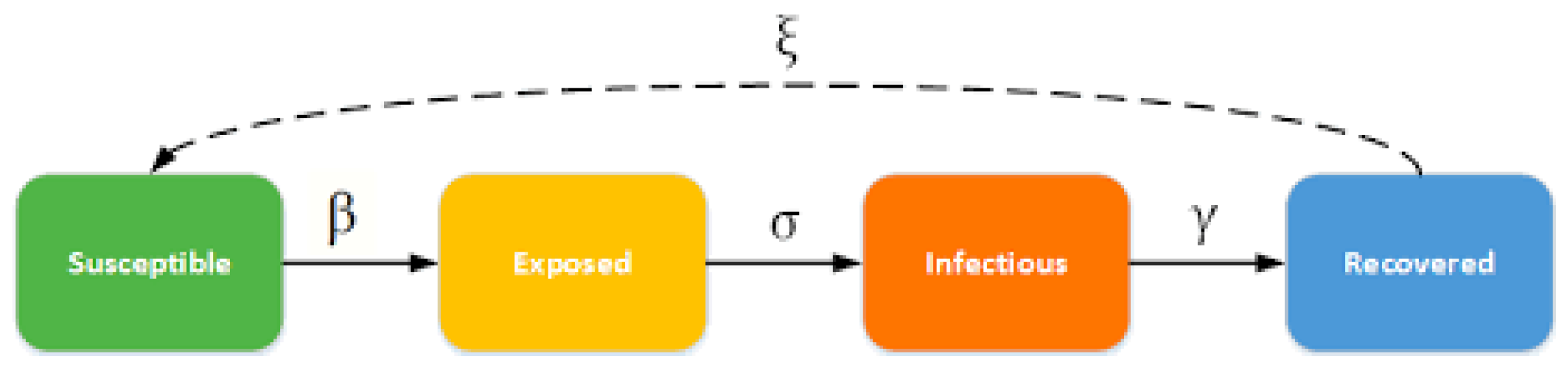
2.3. SEIR Model of COVID-19

The purpose of epidemiological studies is to discover a link between a risk factor and a specific ailment. We utilize a modified version of the SIR model that includes the E class [17]. The susceptible class is represented by an S in the diagram. This class represents the people who are vulnerable to coronavirus infection. Class E, which represents the exposed people, is the part of the population who are infected and has not been detected by testing. Class I, which stands for infectious class, is the class that has been tested and confirmed to be infected by this unique illness. Class R, which stands for recovery, represents the people who have completely recovered from the sickness. Clearly, certain assumptions are involved herein and are be shown in Figure 3.

The assumptions reported above also consider the size of population N, which can be expressed as:

$$N=S+E+I+R.$$

(1)

This population is assumed to be constant in this work. The characteristic equation is used to demonstrate that the population is constant, i.e.,

$$\frac{dN}{dt}=\frac{dS}{dt}+\frac{dE}{dt}+\frac{dI}{dt}+\frac{dR}{dt}=0.$$

(2)

To build our differential equation for class S, we utilize the arrows to represent the rates of flow in and out of the compartments. The rate is positive when an arrow enters the container. When the rate exits the chamber, it is negative. Class S stands for people who are vulnerable to sickness. Class E represents the exposure group. It is the group that is infected with the virus. Class I represents the contagious group. It is the group that has the infection. Class R represents the recovery group, which is the class of people who have either completely recovered or died as a result of the virus.

The path from S to E is the transition of becoming transmitted with COVID-19. Individuals in the exposed class become infected and migrate to the infected class as a result of their risk-taking behavior. Individuals in the exposed group may or may not contract COVID-19. If they do not, persons in the exposed class will be moved to the recovered class after fourteen days of quarantine. Because there is no therapy for COVID-19, there are some people who relocate to class I after recovering from the disease. When an individual has not fully recovered from therapy, they are on the route from I to R. Then, from class R, they shift back into the susceptible class, since they are now more exposed to the virus, and it is easier for the individual to come in contact with it. However, the following differential equations can be used to represent the model at hand [18]:

$$\begin{array}{cc}\hfill & \frac{dS\left(t\right)}{dt}=-\frac{{\alpha }_2}{N}I\left(t\right)S\left(t\right)+{\alpha }_1[N-S\left(t\right)],\hfill \\ \hfill & \frac{dE\left(t\right)}{dt}=-({\alpha }_1+{\alpha }_3)E\left(t\right)+\frac{{\alpha }_2}{N}I\left(t\right)S\left(t\right),\hfill \\ \hfill & \frac{dI\left(t\right)}{dt}=-({\alpha }_1+{\alpha }_4)I\left(t\right)+{\alpha }_{3}E\left(t\right),\hfill \\ \hfill & \frac{dR\left(t\right)}{dt}=-{\alpha }_{1}R\left(t\right)+{\alpha }_{4}I\left(t\right),\hfill \end{array}$$

(3)

where N is the number of the total population, and the parameters ${\alpha }_1$, ${\alpha }_2$, ${\alpha }_3$, and ${\alpha }_4$ represent the parameter of the exposing rate, the parameter of the infection rate, the parameter of recovery rate, and the parameter of mortality rate, respectively. In what follows, we present a new version of the model (3) by fractionalizing the derivative, and hence obtain the so-called fractional-order COVID-19 model which is formulated by operating the Caputo fractional-order derivative operator.

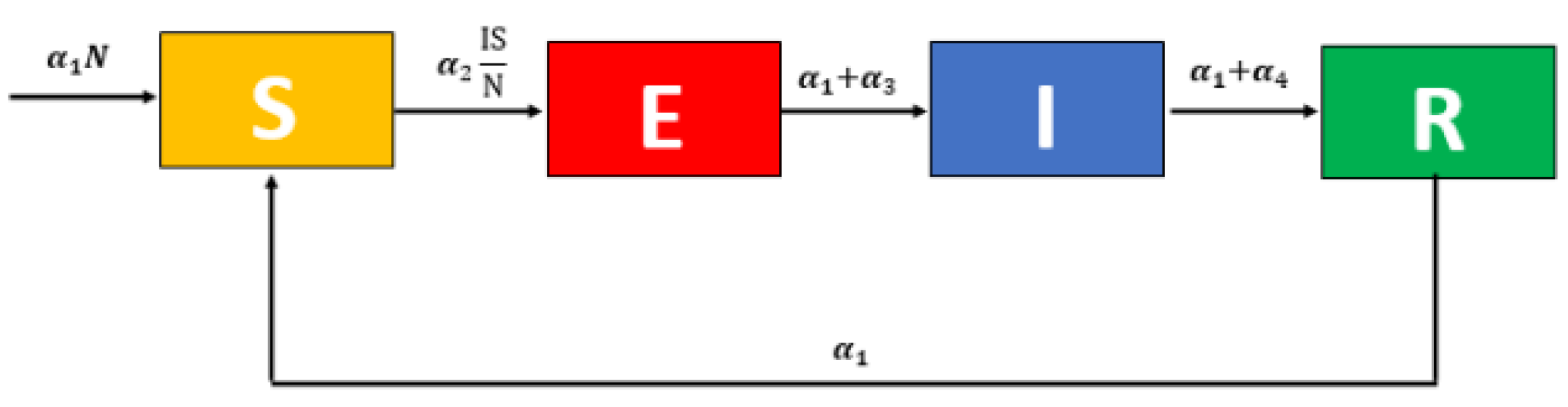
2.4. Fractional-Order COVID-19 Model

In applied mathematics, fractional-order models are connected to binary response models to some extent. Instead of predicting the chance of being in one of two bins of a dichotomous variable, the fractional-order model often works with variables that can take on any value in the unit interval. By using proper transformations, this model may be simply generalized to take on values on any other interval. In recent years, fractional calculus has played an essential role in the domains of mathematics, physics, electronics, mechanics, and engineering. Modeling approaches utilizing fractional operators have been continually developed and improved, particularly in recent decades.

The initial goal of this section is to carry out the Caputo operator on the traditional integer-order COVID-19 model given in (3), in order to create a new nonlinear fractional-order system and, secondly, to provide a certain numerical approach for dealing with such a system. This approach is the Fractional Euler Method (FEM). Anyhow, system (3) can be fictionalized to be as follows:

$$\begin{array}{cc}\hfill & D^{\alpha }S\left(t\right)=-\frac{{\alpha }_2}{N}I\left(t\right)S\left(t\right)+{\alpha }_1[N-S\left(t\right)],\hfill \\ \hfill & D^{\alpha }E\left(t\right)=-({\alpha }_1+{\alpha }_3)E\left(t\right)+\frac{{\alpha }_2}{N}I\left(t\right)S\left(t\right),\hfill \\ \hfill & D^{\alpha }I\left(t\right)=-({\alpha }_1+{\alpha }_4)I\left(t\right)+{\alpha }_{3}E\left(t\right),\hfill \\ \hfill & D^{\alpha }R\left(t\right)=-{\alpha }_{1}R\left(t\right)+{\alpha }_{4}I\left(t\right),\hfill \end{array}$$

(4)

where $D^{\alpha }$ is the Caputo fractional-order derivative operator, $\alpha$ is the fractional-order value, and ${\alpha }_1$, ${\alpha }_2$, ${\alpha }_3$, and ${\alpha }_4$ are the same parameters defined previously in the system (3).

2.5. Stability Analysis

2.5.1. The Equilibrium Small Point of the Model

In order to discuss the fractional-order model (4) in terms of its equilibrium points, it should be noted that there are two major types of such points. The first one is called the Disease-Free Equilibrium (DFE) point, whereas the second point is called the Endemic Equilibrium (EE) point. In particular, to obtain the DFE point, we assume that $I=0$, and the right-hand side of all equations of the ystem (4) are equal to 0. Then, the DFE point of this system is gained to be as follows:

$${\tilde{T}}_{DFE}=(N,0,0,0).$$

(5)

On the other hand, if one considers $I\ne 0$, then the EE is gained as follows:

$$-\frac{{\alpha }_2}{N}IS+{\alpha }_1[N-S]=0.$$

(6)

$$-({\alpha }_1+{\alpha }_3)E+\frac{{\alpha }_2}{N}IS=0.$$

(7)

$$-({\alpha }_1+{\alpha }_4)I+{\alpha }_{3}E=0.$$

(8)

$$-{\alpha }_{1}R+{\alpha }_{4}I=0.$$

(9)

Clearly, based on (8), we can have:

$$E=\frac{{\alpha }_1+{\alpha }_4}{{\alpha }_3}I.$$

(10)

Consequently, if we substitute (10) in (7) and then divide by I, we obtain:

$$S=\frac{N({\alpha }_1+{\alpha }_3)({\alpha }_1+{\alpha }_4)}{{\alpha }_2{\alpha }_3}.$$

(11)

The value of S in (11) can then be substituted in (6) to obtain:

$$I=\frac{{\alpha }_{1}N[{\alpha }_1{\alpha }_3-({\alpha }_1+{\alpha }_3)({\alpha }_1+{\alpha }_4)]}{{\alpha }_2({\alpha }_1+{\alpha }_3)({\alpha }_1+{\alpha }_4)}.$$

(12)

This would immediately provide an expression of E in (10). In other words, we have:

$$E=\frac{{\alpha }_{1}N[{\alpha }_1{\alpha }_3-({\alpha }_1+{\alpha }_3)({\alpha }_1+{\alpha }_4)]}{{\alpha }_2{\alpha }_3\left({\alpha }_1{\alpha }_3\right)}.$$

(13)

Finally, from (9) and (12), we can obtain:

$$R=\frac{{\alpha }_{4}N[{\alpha }_1{\alpha }_3-({\alpha }_1+{\alpha }_3)({\alpha }_1+{\alpha }_4)]}{{\alpha }_2({\alpha }_1+{\alpha }_3)({\alpha }_1+{\alpha }_4)}.$$

(14)

In view of the previous discussion, the EE point can hence be expressed as follows:

$${\tilde{T}}_{EE}=(S_0,E_0,I_0,R_0),$$

where

$$\begin{array}{cc}\hfill & S_0=\frac{N({\alpha }_1+{\alpha }_3)({\alpha }_1+{\alpha }_4)}{{\alpha }_2{\alpha }_3},\hfill \\ \hfill & E_0=\frac{{\alpha }_{1}N[{\alpha }_1{\alpha }_3-({\alpha }_1+{\alpha }_3)({\alpha }_1+{\alpha }_4)]}{{\alpha }_2{\alpha }_3\left({\alpha }_1{\alpha }_3\right)},\hfill \\ \hfill & I_0=\frac{{\alpha }_{1}N[{\alpha }_1{\alpha }_3-({\alpha }_1+{\alpha }_3)({\alpha }_1+{\alpha }_4)]}{{\alpha }_2({\alpha }_1+{\alpha }_3)({\alpha }_1+{\alpha }_4)},\hfill \\ \hfill & R_0=\frac{{\alpha }_{4}N[{\alpha }_1{\alpha }_3-({\alpha }_1+{\alpha }_3)({\alpha }_1+{\alpha }_4)]}{{\alpha }_2({\alpha }_1+{\alpha }_3)({\alpha }_1+{\alpha }_4)}.\hfill \end{array}$$

(15)

Actually, the usefulness of outlining the equilibrium points of the fractional-order COVID-19 model lies in their important role in several stability results related to the basic reproductive number $R_0$, which is handled in the upcoming subsection.

2.5.2. Basic Reproductive Number

In this part, we briefly introduce a capable scheme for calculating the basic reproductive number $R_0^{*}$ that indicates the average number of secondary cases resulting from initial infective cases in a population without disease immunity [19]. Such a critical scale is increasingly being employed as a primary quantity for calculating the force of needed interferences for epidemic control. The overall scheme for computing $R_0^{*}$, which was first established by Diekmann et al. in [20], and then developed by Van den Driessche et al. in [21], can be carried out using the matrix method of the next generation [22]. It is common knowledge in epidemic mathematical modeling that if $R_0^{*}<1$, then there is an absence of epidemics in natural populations. On the contrary, if $R_0^{*}>1$, the disease will then spread rapidly among the vulnerable populations. However, determining such a scale necessitates determining the spectral radius of the next generation matrix or the maximum absolute value of its eigenvalues, (i.e., $R_0^{*}=\rho \left(K\right)$, where K is the next generation matrix). The matrix K typically consists of two components, F and $V^{-1}$, where

$$\begin{array}{cc}\hfill & F=\left[\frac{\partial F_{\mathit{i}}\left({\tilde{T}}_{DFE}\right)}{\partial t_j}\right],V=\left[\frac{\partial V_{\mathit{i}}\left({\tilde{T}}_{DFE}\right)}{\partial t_j}\right],\hfill \end{array}$$

(16)

where $F_{\mathit{i}}$ indicates the flow of newly infected individuals in compartment $z_i$, and $V_i$ indicates the other leaving/entering fluxes associated with the compartment $z_i$ for $i,j=1,2,...,m$, in which m is the number of compartments established in the model.

To find the basic reproductive number, we return to system (4) again and assume the following states:

$$\begin{array}{cc}\hfill & F_1=-\frac{{\alpha }_2}{N}I\left(t\right)S\left(t\right)+{\alpha }_1[N-S\left(t\right)],\hfill \\ \hfill & F_2=-({\alpha }_1+{\alpha }_3)E\left(t\right)+\frac{{\alpha }_2}{N}I\left(t\right)S\left(t\right),\hfill \\ \hfill & F_3=-({\alpha }_1+{\alpha }_4)I\left(t\right)+{\alpha }_{3}E\left(t\right),\hfill \\ \hfill & F_4=-{\alpha }_{1}R\left(t\right)+{\alpha }_{4}I\left(t\right).\hfill \end{array}$$

(17)

Due to $F_1,F_2,F_3$, and $F_4$ of the system (4) describing the generation and the transition of infections, then the Jacobin matrix associated with the linearized subsystem can be obtained according to the following expression:

$$J=\left[\begin{array}{ccccc}\frac{\partial F_1}{\partial S}& \frac{\partial F_1}{\partial E}& & \frac{\partial F_1}{\partial I}& \frac{\partial F_1}{\partial R}\\ \frac{\partial F_2}{\partial S}& \frac{\partial F_2}{\partial E}& & \frac{\partial F_2}{\partial I}& \frac{\partial F_2}{\partial R}\\ \frac{\partial F_3}{\partial S}& \frac{\partial F_3}{\partial E}& & \frac{\partial F_3}{\partial I}& \frac{\partial F_3}{\partial R}\\ \frac{\partial F_4}{\partial S}& \frac{\partial F_4}{\partial E}& & \frac{\partial F_4}{\partial I}& \frac{\partial F_4}{\partial R}\end{array}\right].$$

(18)

Thus, based on (18), we can have:

$$J=\left(\begin{array}{cccc}-\frac{{\alpha }_{2}I}{N}-{\alpha }_1& 0& -\frac{{\alpha }_{2}S}{N}& 0\\ \frac{{\alpha }_{2}I}{N}& -({\alpha }_1+{\alpha }_3)& \frac{{\alpha }_{2}S}{N}& 0\\ 0& {\alpha }_3& -({\alpha }_1+{\alpha }_4)& 0\\ 0& 0& {\alpha }_4& -{\alpha }_4\end{array}\right).$$

(19)

Consequently, we have:

$$J_{{\tilde{T}}_{DFE}}=\left(\begin{array}{cccc}-{\alpha }_1& 0& -{\alpha }_2& 0\\ 0& -({\alpha }_1+{\alpha }_3)& {\alpha }_2& 0\\ 0& {\alpha }_3& -({\alpha }_1+{\alpha }_4)& 0\\ 0& 0& {\alpha }_4& -{\alpha }_4\end{array}\right).$$

(20)

Now, the matrix $J_{{\tilde{T}}_{DFE}}$ can be decomposed as $F-V$, where F is the flux of newly infected cases to compartment I, and V is the fluxes leaving from the compartment I. In other words, we can have:

$$J_{{\tilde{T}}_{DFE}}=\left(\begin{array}{cccc}0& 0& 0& 0\\ 0& 0& {\alpha }_2& 0\\ 0& {\alpha }_3& 0& 0\\ 0& 0& {\alpha }_4& 0\end{array}\right)-\left(\begin{array}{cccc}{\alpha }_1& 0& {\alpha }_2& 0\\ 0& ({\alpha }_1+{\alpha }_3)& 0& 0\\ 0& 0& ({\alpha }_1+{\alpha }_4)& 0\\ 0& 0& 0& {\alpha }_4\end{array}\right),$$

where

$$F=\left(\begin{array}{cccc}0& 0& 0& 0\\ 0& 0& {\alpha }_2& 0\\ 0& {\alpha }_3& 0& 0\\ 0& 0& {\alpha }_4& 0\end{array}\right),$$

and

$$V=\left(\begin{array}{cccc}{\alpha }_1& 0& {\alpha }_2& 0\\ 0& ({\alpha }_1+{\alpha }_3)& 0& 0\\ 0& 0& ({\alpha }_1+{\alpha }_4)& 0\\ 0& 0& 0& {\alpha }_4\end{array}\right).$$

Consequently, we can obtain:

$$V^{-1}=\left(\begin{array}{cccc}\frac{1}{{\alpha }_1}& 0& c& 0\\ 0& \frac{1}{({\alpha }_1+{\alpha }_3)}& 0& 0\\ 0& 0& \frac{1}{({\alpha }_1+{\alpha }_4)}& 0\\ 0& 0& 0& \frac{1}{{\alpha }_4}\end{array}\right),$$

where c is constant. As a result, the next generation matrix K can then be expressed as follows:

$$K=F{V}^{-1}=\left(\begin{array}{cccc}0& 0& 0& 0\\ 0& 0& {\alpha }_2& 0\\ 0& {\alpha }_3& 0& 0\\ 0& 0& {\alpha }_4& 0\end{array}\right)\left(\begin{array}{cccc}\frac{1}{{\alpha }_1}& 0& c& 0\\ 0& \frac{1}{({\alpha }_1+{\alpha }_3)}& 0& 0\\ 0& 0& \frac{1}{({\alpha }_1+{\alpha }_4)}& 0\\ 0& 0& 0& \frac{1}{{\alpha }_4}\end{array}\right),$$

(21)

i.e.,

$$K=\left(\begin{array}{cccc}0& 0& 0& 0\\ 0& 0& \frac{{\alpha }_2}{({\alpha }_1+{\alpha }_4)}& 0\\ 0& \frac{{\alpha }_3}{({\alpha }_4+{\alpha }_3)}& 0& 0\\ 0& 0& \frac{{\alpha }_4}{({\alpha }_1+{\alpha }_4)}& 0\end{array}\right).$$

(22)

This definitely leads us to deduce the final form of $R_0$, which represents the maximum eigenvalue of the matrix K (or the spectral radius of the matrix K), i.e.,

$$R_0^{*}=\rho \left(K\right)=Max\left|\lambda \right|=\frac{{\alpha }_2{\alpha }_3}{({\alpha }_1+{\alpha }_3)({\alpha }_1+{\alpha }_4)},$$

(23)

where $\lambda$ and $\sigma (·)$ are the eigenvalue and the spectrum of the matrix K, respectively.

In the following content, we study the stability of the system (4) according to its DFE point. This result is deemed one of the important results in this work. This is because such results can provide the society under consideration with certain data that can outline when the society is indeed facing epidemics.

Theorem 1. 

The DFE of the system (4) is asymptotically stable if $R_0^{*}<1$ and ${\alpha }_3>{\alpha }_2$.

Proof. 

To show this result, we should be concerned with the Jacobian matrix again at DFE. To this aim, we can find the characteristic equation by considering the following equation:

$$det(\lambda I-J_{{\tilde{T}}_{DFE}})=0.$$

(24)

This immediately implies:

$$\left|\begin{array}{cccc}\lambda +{\alpha }_1& 0& {\alpha }_2& 0\\ 0& \lambda +{\alpha }_1+{\alpha }_3& -{\alpha }_2& 0\\ 0& -{\alpha }_3& \lambda +{\alpha }_1+{\alpha }_4& 0\\ 0& 0& -{\alpha }_4& \lambda +{\alpha }_4\end{array}\right|=0.$$

As a result, we can reach the following equation:

$$(\lambda +{\alpha }_1)\times [(\lambda +{\alpha }_1+{\alpha }_3)(\lambda +{\alpha }_1+{\alpha }_4)(\lambda +{\alpha }_4)+{\alpha }_2(-{\alpha }_3(\lambda +{\alpha }_4))]=0.$$

(25)

After performing some long calculations, we can directly obtain all eigenvalues of the matrix $J_{{\tilde{T}}_{DFE}}$ to be as follows:

$$\begin{array}{cc}\hfill & {\lambda }_1=-{\alpha }_1,{\lambda }_2=-{\alpha }_4\hfill \\ \hfill & {\lambda }_3=\frac{-(2{\alpha }_1+{\alpha }_3+{\alpha }_4)-\sqrt{{({\alpha }_3-{\alpha }_4)}^2+4{\alpha }_2{\alpha }_3}}{2},\hfill \\ \hfill & {\lambda }_4=\frac{-(2{\alpha }_1+{\alpha }_3+{\alpha }_4)+\sqrt{{({\alpha }_3-{\alpha }_4)}^2+4{\alpha }_2{\alpha }_3}}{2}\hfill \end{array}$$

(26)

Obviously, ${\lambda }_i<0$, for $i=1,2,3$. Now, it remains to show that ${\lambda }_4<0$. For this purpose, we use the assumption $R_0^{*}<1$. That is, due to ${\alpha }_i>0$, for $i=1,2,3,4$, then:

$$\frac{{\alpha }_2{\alpha }_3}{({\alpha }_1+{\alpha }_3)({\alpha }_1+{\alpha }_4)}<1.$$

This consequently implies:

$${\alpha }_2{\alpha }_3<({\alpha }_1+{\alpha }_3)({\alpha }_1+{\alpha }_4).$$

(27)

By inserting (27) into the expression of ${\lambda }_4$, we obtain:

$${\lambda }_4<\frac{-(2{\alpha }_1+{\alpha }_3+{\alpha }_4)+\sqrt{{\alpha }_3^2-2{\alpha }_3{\alpha }_4+{\alpha }_4^2+4({\alpha }_1+{\alpha }_3)({\alpha }_1+{\alpha }_4)}}{2}.$$

After performing some long calculations, we can obtain the following inequality:

$${\lambda }_4<\frac{-(2{\alpha }_1+{\alpha }_3+{\alpha }_4)+\sqrt{{({\alpha }_3+{\alpha }_4)}^2+4({\alpha }_1^2+{\alpha }_1{\alpha }_3+{\alpha }_1{\alpha }_4)}}{2}.$$

From this point of view, it suffices to prove that:

$$(2{\alpha }_1+{\alpha }_3+{\alpha }_4)>\sqrt{{({\alpha }_3+{\alpha }_4)}^2+4({\alpha }_1^2+{\alpha }_1{\alpha }_2+{\alpha }_1{\alpha }_4)}.$$

For this purpose, we suppose by contrary that this claim is not true. This would assert:

$$(2{\alpha }_1+{\alpha }_3+{\alpha }_4)<\sqrt{{({\alpha }_3+{\alpha }_4)}^2+4({\alpha }_1^2+{\alpha }_1{\alpha }_2+{\alpha }_1{\alpha }_4)},$$

or

$${(2{\alpha }_1+{\alpha }_3+{\alpha }_4)}^2<{({\alpha }_3+{\alpha }_4)}^2+4({\alpha }_1^2+{\alpha }_1{\alpha }_2+{\alpha }_1{\alpha }_4).$$

Performing some long calculations yields the following inequality:

$$4{\alpha }_1{\alpha }_3<4{\alpha }_1{\alpha }_2.$$

Consequently, we have:

$${\alpha }_3<{\alpha }_2,$$

which is a contradiction to our assumption, and hence ${\lambda }_4<0$. This conclusion confirms that all eigenvalues of matrix $J_{{\tilde{T}}_{DFE}}$ are negative, validating that the DFE point of system (4) is indeed asymptotically stable. □

3. Solving Fractional-Order COVID-19 Model Using Fractional Euler Method

In this section, we aim to solve the fractional-order COVID-19 model numerically. This is performed by using the fractional Euler method which was proposed in [23,24]. Actually, many researchers are interested in developing mathematical models based on fractional-order differential equations see [25,26,27,28,29,30], as they represent important apparatuses for studying memory and some hereditary aspects of many biological components, as well as also being closely related to the fractal theory. In particular, generalizing a classical mathematical model to a fractional-order version allows for gaining more degrees of freedom. It can also integrate the memory effect of the traditional one. These are the primary benefits of fractional-order derivatives, rather than ordinary-order derivatives. As a result, the fractional-order derivatives have a more lifelike appearance than regular derivatives.

3.1. Fractional Euler Method

In this subsection, we introduce the fractional Euler method in view of the Caputo operator, which represents a generalized numerical scheme for the well-known Euler scheme. However, before that, we introduce a generalized Taylor’s theorem in the sense of the Caputo operator, which is deemed as a generalization of the traditional Taylor theorem.

Theorem 2. 

Suppose that $D^{ka}g\left(x\right)\in C(0,a]$ for k = 0, 1, 2, ..., n + 1, where $0<\alpha \le 1$. Then, we have:

$$g\left(x\right)=\sum _{i=0}^n\frac{x^{i\alpha }}{\mathsf{\Gamma }(i\alpha +1)}\left(D^{i\alpha }g\left(0\right)\right)(0+)+\frac{\left(D^{(n+1)\alpha }g\right)\left(\xi \right)}{\mathsf{\Gamma }\left(\right(n+1)\alpha +1)}{x}^{(n+1)\alpha }.$$

In order to illustrate the fractional Euler method that can be implemented numerically to solve the initial value problem with Caputo fractional-order derivative operator, one should note that such a method is a generalization of the classical Euler method. To this aim, we consider the following initial value problem:

$$D^{\alpha }y\left(t\right)=g(t,y\left(t\right)),y\left(0\right)=y_0,0<\alpha \le 1,t>0.$$

(28)

To deal with the above problem, we let $[0,a]$ be the interval over which we want to find the solution to the problem (28). In reality, we will not be able to find a function $y\left(t\right)$ that solves the problem (28). Instead, we generate a set of points $(t_i,y\left(t_i\right))$ and utilize the points for our approximation.

For convenience, we subdivide the interval $[0,a]$ into k subintervals $[t_j,t_{j+1}]$ of equal width $h=a/k$ by using the nodes $t_j=jh$ for $j=0,1,2,...,k$. Assume that $y\left(t\right)$, $D^{\alpha }y\left(t\right)$ and $D^{2\alpha }y\left(t\right)$ are continuous on $[0,a]$ and use the generalized Taylor’s formula to expand $y\left(t\right)$ about $t=t_0=0$. For each value t, there is a value $c_1$, so that:

$$y\left(t\right)=y\left(t_0\right)+\left(D^{\alpha }y\left(t\right)\right)\left(t_0\right)\frac{t^{\alpha }}{\mathsf{\Gamma }(\alpha +1)}+\left(D^{2\alpha }y\left(t\right)\right)\left(c_1\right)\frac{t^{2\alpha }}{\mathsf{\Gamma }(2\alpha +1)}.$$

(29)

When $\left(D^{\alpha }y\left(t\right)\right)\left(t_0\right)=g(t_0,y\left(t_0\right))$ and $h=t_1$ are substituted into Equation (29), the result of an expression for $y\left(t_1\right)$ will be then gained, i.e.,

$$y\left(t_1\right)=y\left(t_0\right)+g(t_0,y\left(t_0\right))\frac{h^{\alpha }}{\mathsf{\Gamma }(\alpha +1)}+\left(D^{2\alpha }y\left(t\right)\right)\left(c_1\right)\frac{h^{2\alpha }}{\mathsf{\Gamma }(2\alpha +1)}.$$

(30)

If one chooses a step size h small enough, then we may eliminate the second-order term of Equation (30) to obtain:

$$y\left(t_1\right)=y\left(t_0\right)+\frac{h^{\alpha }}{\mathsf{\Gamma }(\alpha +1)}g(t_0,y\left(t_0\right)).$$

(31)

This process is continued until a series of points is generated that approximates the aimed solution $y\left(t\right)$. The general formula for the fractional Euler method can then be outlined as follows:

$$\begin{array}{cc}\hfill & t_{j+1}=t_j+h,\hfill \\ \hfill & y\left(t_{j+1}\right)=y\left(t_j\right)+hg(t_j,y\left(t_j\right)),\hfill \end{array}$$

(32)

for $j=0,1,2,...,k-1$. It is clear that if $\alpha =1$, then the fractional Euler method (32) reduces to the classical Euler method.

3.2. Simulations of Fractional-Order COVID-19 Model

In this section, we use the fractional Euler method to solve the system (4). For this purpose, we can consider such a system again as follows:

$$\begin{array}{cc}\hfill & D^{\alpha }S\left(t\right)=g_1(t,S\left(t\right),E\left(t\right),I\left(t\right),R\left(t\right)),\hfill \\ \hfill & D^{\alpha }E\left(t\right)=g_2(t,S\left(t\right),E\left(t\right),I\left(t\right),R\left(t\right)),\hfill \\ \hfill & D^{\alpha }I\left(t\right)=g_3(t,S\left(t\right),E\left(t\right),I\left(t\right),R\left(t\right)),\hfill \\ \hfill & D^{\alpha }R\left(t\right)=g_4(t,S\left(t\right),E\left(t\right),I\left(t\right),R\left(t\right)),\hfill \end{array}$$

(33)

where

$$\begin{array}{cc}\hfill & g_1(t,S\left(t\right),E\left(t\right),I\left(t\right),R\left(t\right))=-\frac{{\alpha }_2}{N}I\left(t\right)S\left(t\right)+{\alpha }_1[N-S\left(t\right)],\hfill \\ \hfill & g_2(t,S\left(t\right),E\left(t\right),I\left(t\right),R\left(t\right))=-({\alpha }_1+{\alpha }_3)E\left(t\right)+\frac{{\alpha }_2}{N}I\left(t\right)S\left(t\right),\hfill \\ \hfill & g_3(t,S\left(t\right),E\left(t\right),I\left(t\right),R\left(t\right))=-({\alpha }_1+{\alpha }_4)I\left(t\right)+{\alpha }_{3}E\left(t\right),\hfill \\ \hfill & g_4(t,S\left(t\right),E\left(t\right),I\left(t\right),R\left(t\right))=-{\alpha }_{1}R\left(t\right)+{\alpha }_{4}I\left(t\right).\hfill \end{array}$$

For instance, in order to generate the set of points $\{t_k,S\left(t_k\right)\}$ of the class S formulated in such a system, we have to assume that each $S\left(t\right)$, $D^{\alpha }S\left(t\right)$, and $D^{2\alpha }S\left(t\right)$ are continuous on [0, T]. In this regard, if one supposes that $g_1(t,S\left(t\right))$=$-\frac{{\alpha }_2}{N}I\left(t\right)S\left(t\right)+{\alpha }_1[N-S\left(t\right)]$, and expands $D^{\alpha }S\left(t\right)=g(t,S\left(t\right))$ about $t_0=0$ by using the generalized Taylor’s formula, we obtain to the following expression:

$$S\left(t\right)=S\left(t_0\right)+\frac{h^{\alpha }}{\mathsf{\Gamma }(\alpha +1)}\left(D^{\alpha }S\left(t\right)\right)\left(t_0\right)+\frac{h^{2\alpha }}{\mathsf{\Gamma }(2\alpha +1)}\left(D^{2\alpha }S\left(t\right)\right)\left(c_1\right),\forall t,$$

(34)

where $c_1$ is an arbitrary constant. Ignoring the term $\frac{h^{2\alpha }}{\mathsf{\Gamma }(2\alpha +1)}\left(D^{2\alpha }S\left(t\right)\right)\left(c_1\right)$ by picking up a quite small step size h, and then substituting $\left(D^{\alpha }S\left(t\right)\right)\left(t_0\right)=g(t_0,S\left(t_0\right))$ together with $h=t_1$ into (34), yields a new expression for $S\left(t_1\right)$ of the form:

$$S\left(t_1\right)=S\left(t_0\right)+\frac{t_1^{\alpha }}{\mathsf{\Gamma }(\alpha +1)}g(t_0,S\left(t_0\right)).$$

(35)

This approach, of course, maybe iterated k-times, yielding the following explicit formula, which yields an approximate solution to $S\left(t\right)$:

$$S\left(t_{k+1}\right)=S\left(t_k\right)+\frac{t^{\alpha }}{\mathsf{\Gamma }(\alpha +1)}(-\frac{{\alpha }_2}{N}I\left(t\right)S\left(t\right)+{\alpha }_1[N-S\left(t\right)]),$$

(36)

where $t_{k+1}=t_k+h$ and $k=0,1,2,...,\ell -1$.

Similarly, the procedure outlined above can be used to obtain approximate numerical solutions for additional classes. Ultimately, we deduce the recursive states that represent the whole approximate numerical solution of the system (33):

$$\begin{array}{cc}\hfill & S\left(t_{k+1}\right)=S\left(t_k\right)+\frac{t^{\nu }}{\mathsf{\Gamma }(\nu +1)}(-\frac{{\alpha }_2}{N}I\left(t\right)S\left(t\right)+{\alpha }_1[N-S\left(t\right)]),\hfill \\ \hfill & E\left(t_{k+1}\right)=E\left(t_k\right)+\frac{t^{\nu }}{\mathsf{\Gamma }(\nu +1)}(-({\alpha }_1+{\alpha }_3)E\left(t\right)+\frac{{\alpha }_2}{N}I\left(t\right)S\left(t\right)),\hfill \\ \hfill & I\left(t_{k+1}\right)=I\left(t_k\right)+\frac{t^{\nu }}{\mathsf{\Gamma }(\nu +1)}(-({\alpha }_1+{\alpha }_4)I\left(t\right)+{\alpha }_{3}E\left(t\right)),\hfill \\ \hfill & R\left(t_{k+1}\right)=R\left(t_k\right)+\frac{t^{\nu }}{\mathsf{\Gamma }(\nu +1)}(-{\alpha }_{1}R\left(t\right)+{\alpha }_{4}I\left(t\right)),\hfill \end{array}$$

(37)

where $k=0,1,2,...,\ell -1.$

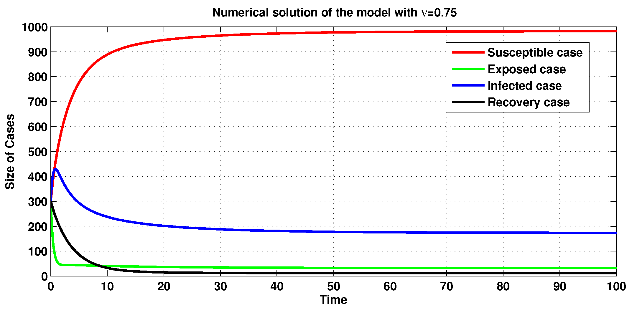
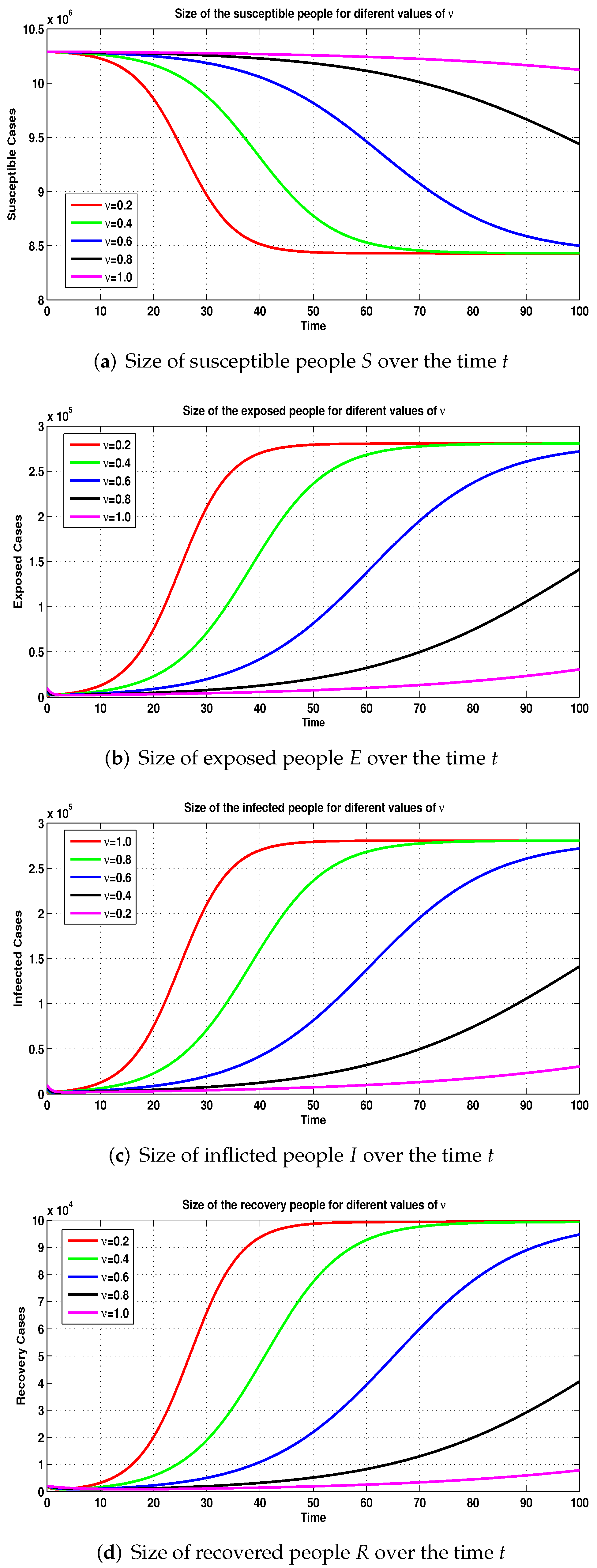
3.3. Numerical Simulations

In this part, we introduce some numerical simulations that illustrate what the proposed fractional-order COVID-19 looks like. In particular, we first present a graphical numerical solution of our proposed model in the sense of the Caputo operator by considering $\alpha =0.75$; several numerical simulations of susceptible, exposed, infected, and recovered people are also illustrated by taking different fractional-order values, and finally, a numerical comparison between the infected size gained from three stems is performed graphically. These stems are the infected results obtained from real data, the obtained results from the classical model, and finally, the obtained results from our COVID-19 model.

In this work, all numerical simulations are performed by using the MATLAB software package according to the initial values reported in

Table 1. The initial value of the classes of the model (4).

Class	Initial Value
S (0)	10,287,128
E (0)	10,000
I (0)	872
R (0)	2000

and to the values of parameters reported in

Table 2. The initial value of the classes of the model (4).

Parameter	Value
${\alpha }_1$	0.15
${\alpha }_2$	0.23
${\alpha }_3$	0.85
${\alpha }_4$	0.01

. As a matter of fact, the values declared in Table 2 were collected from some real data provided by the Ministry of Health in Jordan over 40 days, from 1 January 2022 up to 10 February 2022.

In order to highlight the numerical solution of the fractional-order COVID-19 model given in (6), obtained by using the fractional Euler method, Figure 4 shows the susceptible, exposed, infected, and recovered classes’ behavior over 100 days, along with taking the fractional-order value $\alpha =0.75$.

Here, we can observe that a symmetrical aspect appears in the susceptible and recovered subpopulations. In order to see how the approximate solutions for all classes of our proposed model look, Figure 5a–c illustrate such solutions that represent the whole size for each susceptible, exposed, infected, and recovered person over the time t. These figures are generated in light of several fractional-order values. In particular, Figure 5a represents the size of the susceptible people, which shows their decreasing state over 100 days. Figure 5b shows that the exposed cases are expected to be increasing over the same period. The infected cases are shown in Figure 5c, in which they are expected to also be increased. Finally, the recovery of people is expected to be increased over time, as shown in Figure 5d.

By viewing the above figures, one can see that any change in the fractional-order values has an effect on the present illness phase given in (7), confirming the presence of great degrees of freedom for such a proposed model.

With the aim of evaluating the performance of the fractional-order model (4) and its impacts, we make certain predictions by using such a proposed system based on a numerical comparison that was performed between its dynamics and some real data collected from Jordanian society over 40 days; from 1 January 2022 up to 10 February 2022, (see https:corona.moh.gov.jo/ar). Actually, this numerical compassion, which can be shown in Figure 6, is considered one of the main focuses of this work. For instance, Figure 6 reveals that the fractional-order COVID-19 model (4) is better than the traditional integer-order model (3), especially when we make a comparison between its dynamics and certain real data collected throughout the mentioned period. In other words, we note that these data aggregate and come closer to the infected cases curve of the system (4) more than they aggregate and come closer to the infected cases curve of the system (3). This means that the fractional-order model (4) formulated at $\alpha =0.91$ has proved its efficiency in describing the dynamics of the infected cases against the integer-order system (3). This outcome will undoubtedly enable specialists to predict the number of infected cases that may be correctly detected in the whole of a society, and hence allow decision makers and influencers to set the right plans and logical strategies that should be followed to face this pandemic.

4. Conclusions

The growth of COVID-19 dynamics applied to Jordan during a 40-day period, from 1 January 2022 to 10 February 2022, was suggested and examined in this study using a novel nonlinear fractional-order COVID-19 model. The dynamics of the established model were effectively simulated using the Fractional Euler Method (FEM). The fractional-order COVID-19 models were shown to be superior to the classical ones through some numerical comparisons because of what these models showed in comparison with some real data gathered from Jordanian culture. As a consequence, it can be concluded that the suggested fractional-order model is more effective than the integer-order one at predicting the development of COVID-19 dynamics. This conclusion can help key decision makers and influencers establish the appropriate plans and sensible courses of action to take in order to face a pandemic.

References

1. Tymoczko, D. A Geometry of Music: Harmony and Counterpoint in the Extended Common Practice; Oxford University Press: Oxford, UK, 2010. [Google Scholar]
2. Kornai, A. Mathematical Linguistics; Springer Science & Business Media: Berlin/Heidelberg, Germany, 2007. [Google Scholar]
3. Mišutka, J.; Galamboš, L. System description: Egomath2 as a tool for mathematical searching on Wikipedia. org. In Proceedings of the International Conference on Intelligent Computer Mathematics, Bertinoro, Italy, 18–23 July 2011; Springer: Berlin/Heidelberg, Germany, 2011; pp. 307–309. [Google Scholar]
4. Khan, T.; Ahmad, S.; Ullah, R.; Bonyah, E.; Ansari, K.J. The asymptotic analysis of novel coronavirus disease via fractional-order epidemiological model. AIP Adv. 2022, 12, 035349. [Google Scholar] [CrossRef]
5. Ahmad, S.; Owyed, S.; Abdel-Aty, A.H.; Mahmoud, E.E.; Shah, K.; Alrabaiah, H. Mathematical analysis of COVID-19 via new mathematical model. Chaos Solitons Fractals 2021, 143, 110585. [Google Scholar]
6. Ullah, A.; Ahmad, S.; ur Rahman, G.; Alqarni, M.M.; Mahmoud, E.E. Impact of pangolin bootleg market on the dynamics of COVID-19 model. Results Phys. 2021, 23, 103913. [Google Scholar] [CrossRef] [PubMed]
7. Liu, X.; Rahmamn, M.u.; Ahmad, S.; Baleanu, D.; Anjam, Y.N. A new fractional infectious disease model under the non-singular Mittag–Leffler derivative. Waves Random Complex Media 2022, 1–27. [Google Scholar] [CrossRef]
8. Ahmad, S.; Ullah, R.; Baleanu, D. Mathematical analysis of tuberculosis control model using nonsingular kernel type Caputo derivative. Adv. Differ. Equ. 2021, 2021, 26. [Google Scholar] [CrossRef]
9. Bezziou, M.; Dahmani, Z.; Jebril, I.; Kaid, M. Caputo-hadamard approach applications: Solvability for an integro-differential problem of lane and emden type. J. Math. Comput. Sci. 2021, 11, 1629–1649. [Google Scholar]
10. Tanimoto, J. Sociophysics Approach to Epidemics; Springer: Singapore, 2021; Volume 23, pp. 153–169. [Google Scholar]
11. Omame, A.; Abbas, M.; Onyenegecha, C.P. A fractional-order model for COVID-19 and tuberculosis co-infection using Atangana–Baleanu derivative. Chaos Solitons Fractals 2021, 153, 111486. [Google Scholar] [CrossRef]
12. Kermack, W.O.; Mckendrick, A.G. A contribution to the mathematical theory of epidemics. Proc. R. Soc. London. Ser. A Contain. Pap. Math. Phys. Character 1927, 115, 700–721. [Google Scholar]
13. Wirkus, S.A.; Swift, R.J. A Course in Ordinary Differential Equations; CRC Press: Boca Raton, FL, USA, 2006. [Google Scholar]
14. Cobb, N.L.; Sathe, N.A.; Duan, K.I.; Seitz, K.P.; Thau, M.R.; Sung, C.C.; Morrell, E.D.; Mikacenic, C.; Kim, H.N.; Liles, W.C.; et al. Comparison of clinical features and outcomes in critically ill patients hospitalized with COVID-19 versus influenza. Ann. Am. Thorac. Soc. 2021, 18, 632–640. [Google Scholar] [CrossRef]
15. Eppes, H. A Seir Mathematical Model of SAR-CoV-2. Ph.D. Thesis, Elizabeth City State University, Elizabeth City, NC, USA, 2021. [Google Scholar]
16. Wald, E.R.; Schmit, K.M.; Gusland, D.Y. A pediatric infectious disease perspective on COVID-19. Clin. Infect. Dis. 2021, 72, 1660–1666. [Google Scholar] [CrossRef]
17. Singh, P.S.K.; Arora, U. Stability of seir model of infectious diseases with human immunity. Glob. J. Pure Appl. Math. 2017, 13, 1811–1819. [Google Scholar]
18. Al-Raeei, M. The forecasting of covid-19 with mortality using sird epidemic model for the United States, Russia, China, and the Syrian Arab republic. AIP Adv. 2020, 10, 065325. [Google Scholar] [CrossRef]
19. Pengpeng, S.; Shengi, C.; Peihua, F. Seir transmission dynamics model of 2019 nCoV coronavirus with considering the weak infectious ability and changes in latency duration. MedRxiv 2020. [Google Scholar] [CrossRef]
20. Diekmann, O.; Heesterbeek, J.A.P.; Metz, J.A. On the definition and the computation of the basic reproduction ratio r 0 in models for infectious diseases in heterogeneous populations. J. Math. Biol. 1990, 28, 365–382. [Google Scholar] [CrossRef] [Green Version]
21. Van den Driessche, P. Reproduction numbers and sub-threshold endemic equilibria for compartmental models of disease transmission. Math. Biosci. 2002, 180, 29–48. [Google Scholar] [CrossRef]
22. Van den Driessche, P. Reproduction numbers of infectious disease models. Infect. Dis. Model. 2017, 2, 288–303. [Google Scholar] [CrossRef]
23. Odibat, Z.M.; Shawagfeh, N.T. Generalized taylor’s formula. Appl. Math. Comput. 2007, 186, 286–293. [Google Scholar] [CrossRef]
24. Dahmani, Z.; Anber, A.; Jebril, I. Solving Conformable Evolution Equations by an Extended Numerical Method. Jordan J. Math. Stat. 2022, 15, 363–380. [Google Scholar]
25. Debbouche, N.; Ouannas, A.; Batiha, I.M.; Grassi, G. Chaotic dynamics in a novel COVID-19 pandemic model described by commensurate and incommensurate fractional-order derivatives. Nonlinear Dyn. 2021, 109, 33–45. [Google Scholar] [CrossRef]
26. Albadarneh, R.B.; Batiha, I.M.; Ouannas, A.; Momani, S. Modeling COVID-19 pandemic outbreak using fractional-order systems. Int. J. Math. Comput. Sci. 2021, 16, 1405–1421. [Google Scholar]
27. Batiha, I.M.; Momani, S.; Ouannas, A.; Momani, Z.; Hadid, S.B. Fractional-order COVID-19 pandemic outbreak: Modeling and stability analysis. Int. J. Biomath. 2022, 15, 2150090. [Google Scholar] [CrossRef]
28. Djenina, N.; Ouannas, A.; Batiha, I.M.; Grassi, G.; Oussaeif, T.E.; Momani, S. A Novel Fractional-Order Discrete SIR Model for Predicting COVID-19 Behavior. Mathematics 2022, 10, 2224. [Google Scholar] [CrossRef]
29. Batiha, I.M.; Al-Nana, A.A.; Albadarneh, R.B.; Ouannas, A.; Al-Khasawneh, A.; Momani, S. Fractional-order coronavirus models with vaccination strategies impacted on Saudi Arabia’s infections. AIMS Math. 2022, 7, 12842–12858. [Google Scholar] [CrossRef]
30. Batiha, I.M.; Alshorm, S.; Ouannas, A.; Momani, S.; Ababneh, O.Y.; Albdareen, M. Modified Three-Point Fractional Formulas with Richardson Extrapolation. Mathematics 2022, 10, 3489. [Google Scholar] [CrossRef]
Figure 1. Illustration of SIR model.
Symmetry 14 02583 g001
Figure 2. Illustration of SEIR model and its four components.
Symmetry 14 02583 g002
Figure 3. Compartment diagram of the SEIR model considered in this study.
Symmetry 14 02583 g003
Figure 4. The numerical solution of model (4).
Symmetry 14 02583 g004
Figure 5. Size of all classes over the time t (in days) for system (4) in view of different values of α using FMEM.
Symmetry 14 02583 g005
Figure 6. Comparison between the infected size gained from the proposed model and real data.
Symmetry 14 02583 g006