A Simplification and Generalization of Elsayed and Ibrahim’s Two-Dimensional System of Third-Order Difference Equations

Abstract

A full Lie analysis of a system of third-order difference equations is performed. Explicit solutions, expressed in terms of the initial values, are derived. Furthermore, we give sufficient conditions for the existence of two-periodic and four-periodic solutions in certain cases. Our results generalize and simplify some work in the literature.

1. Introduction

The area of difference equations has attracted many researchers recently (see [1,2,3,4,5,6]). Methods for solving difference equations have been developed (see [7,8,9,10,11,12,13,14,15]) and the Lie symmetry approach is one of them. One of the most useful algorithms for computing the symmetries of difference equations is due to Hydon (see [12]). The Lie symmetry group of a system of difference equations is the largest group of point transformations acting on the space of dependent and independent variables that leave the equations unchanged. Thus, an element of such a group maps a solution of the difference equation onto another solution. In this method, the order of the difference equation is reduced, and using the invariance of the equation under group transformations or via the similarity variables, one can find the exact solutions. For more on symmetries, conservation laws and invariants, refer to [16,17].

In this paper, by applying the Lie symmetry method, we generalize some results in [18], where Elsayed and Ibrahim investigated the periodic nature and the form of the solutions of a nonlinear system of difference equations of order three:

$$\begin{array}{c}\hfill x_{n+1}=\frac{x_{n-2}{y}_{n-1}}{y_n(\pm 1\pm 1x_{n-2}{y}_{n-1})},y_{n+1}=\frac{y_{n-2}{x}_{n-1}}{x_n(\pm 1\pm 1y_{n-2}{x}_{n-1})}.\end{array}$$

(1)

We study the system

$$\begin{array}{c}\hfill x_{n+1}=\frac{x_{n-2}{y}_{n-1}}{y_n(a_n+b_n{x}_{n-2}{y}_{n-1})},y_{n+1}=\frac{y_{n-2}{x}_{n-1}}{x_n(c_n+d_n{y}_{n-2}{x}_{n-1})},\end{array}$$

(2)

where ${\left(a_n\right)}_{n\in {\mathbb{Z}}_{\ge 0}},{\left(b_n\right)}_{n\in {\mathbb{Z}}_{\ge 0}}$ are non-zero real sequences, and $x_{-2},x_{-1},x_0,y_{-2},y_{-1}$ and $y_0$ are initial values. Because of the definitions and notation we want to use, we study the equivalent system

$$\begin{array}{c}\hfill x_{n+3}=\frac{x_n{y}_{n+1}}{y_{n+2}(A_n+B_n{x}_n{y}_{n+1})},y_{n+3}=\frac{y_n{x}_{n+1}}{x_{n+2}(C_n+D_n{y}_n{x}_{n+1})},\end{array}$$

(3)

where ${\left(A_n\right)}_{n\in {\mathbb{Z}}_{\ge 0}},{\left(B_n\right)}_{n\in {\mathbb{Z}}_{\ge 0}}$ are non-zero real sequences.

In coming up with the solutions of (2) using the Lie symmetry method, we first find the Lie algebra of (2). We then reduce the order of the equations by utilizing the invariants and later use iterations to deduce the solutions.

Preliminaries

In this section, we give the background of the Lie symmetry analysis. The notation used comes from [12].

Definition 1

([19]). Let G be a local group of transformations acting on a manifold M. A subset $\mathcal{S}\subset M$ is called G-invariant, and G is called symmetry group of $\mathcal{S}$, if whenever $x\in \mathcal{S}$, and $g\in G$ is such that $g·x$ is defined, then $g·x\in \mathcal{S}$.

Definition 2

([19]). Let G be a connected group of transformations acting on a manifold M. A smooth real-valued function $\zeta :M\to \mathbb{R}$ is an invariant function for G if and only if

$$X\left(\zeta \right)=0\mathit{for}\mathit{all}x\in M,$$

and every infinitesimal generator X of G.

Definition 3

([12]). A parameterized set of point transformations,

$${\Gamma }_{\epsilon }:x\mapsto \widehat{x}(x;\epsilon ),$$

(4)

where $x=x_i,$$i=1,\cdots ,p$ are continuous variables, is a one-parameter local Lie group of transformations if the following conditions are satisfied:

1.

${\Gamma }_0$ is the identity map if $\widehat{x}=x$ when $\epsilon =0$.

2.

${\Gamma }_a{\Gamma }_b={\Gamma }_{a+b}$ for every a and b sufficiently close to 0.

3.

Each $\widehat{x_i}$ can be represented as a Taylor series (in a neighborhood of $\epsilon =0$ that is determined by x), and therefore

$$\widehat{x_i}(x:\epsilon )=x_i+\epsilon {\xi }_i\left(x\right)+O\left({\epsilon }^2\right),i=1,...,p.$$

(5)

Consider the system of ordinary difference equations

$$\begin{array}{c}\hfill \left\{\begin{array}{cc}{x}_{n+3}=\hfill & {\Omega }_1(x_n,x_{n+1},x_{n+2},y_n,y_{n+1},y_{n+2}),\hfill \\ y_{n+3}=\hfill & {\Omega }_2(x_n,x_{n+1},x_{n+2},y_n,y_{n+1},y_{n+2}),n\in D\hfill \end{array}\right.\end{array}$$

(6)

for some smooth function $\Omega =({\Omega }_1,{\Omega }_2)$ and a regular domain $D\subset \mathbb{Z}$. To find a symmetry group of (6), we consider the group of infinitesimal point transformations given by

$$G_{\epsilon }:(x_n,y_n)\mapsto (x_n+\epsilon Q_1(n,x_n),y_n+\epsilon Q_2(n,y_n)),$$

(7)

where $\epsilon$ is the parameter and $Q_i,i=1,2$, the continuous functions which we shall refer to as characteristics. Let

$$\begin{array}{cc}\hfill \mathcal{X}=& Q_1(n,x_n)\frac{\partial }{\partial x_n}+Q_2(n,y_n)\frac{\partial }{\partial y_n}\hfill \end{array}$$

(8)

be the corresponding infinitesimal generator of $G_{\epsilon }$ with the k-th extension

$$X=Q_1\frac{\partial }{\partial x_n}+Q_2\frac{\partial }{\partial y_n}+S{Q}_1\frac{\partial }{\partial x_{n+1}}+S{Q}_2\frac{\partial }{\partial y_{n+1}}+S^2{Q}_1\frac{\partial }{\partial x_{n+2}}+S^2{Q}_2\frac{\partial }{\partial y_{n+2}}.$$

(9)

Note that S is the forward shift operator, acting on n as follows: $S:n\to n+1$. Further, the linearized symmetry conditions are given by

$$\begin{array}{c}\hfill {\mathcal{S}}^{\left(3\right)}{Q}_1-X{\Omega }_1=0,{\mathcal{S}}^{\left(3\right)}{Q}_2-X{\Omega }_2=0.\end{array}$$

(10)

Once a characteristic $Q_i$ is known, the invariant ${\zeta }_i$ may be obtained by introducing the canonical coordinate [20]

$$\begin{array}{c}\hfill s_n=\int \frac{d{x}_n}{Q_1(n,x_n)}\mathrm{and}{t}_n=\int \frac{d{y}_n}{Q_2(n,y_n)}.\end{array}$$

(11)

In general, the constraints on the constants in the characteristics give one a clear idea (without any lucky guess) about the perfect choice of invariants.

The paper is organized as follows: In Section 2, we discuss the symmetries, reductions and exact solutions of (3). In Section 3, we look at the solutions of (2), and in Section 4, we discuss the periodicity of some solutions.

2. Symmetries, Reductions and Exact Solutions of (3)

Consider the system (3), that is,

$$\begin{array}{c}\hfill x_{n+3}=\frac{x_n{y}_{n+1}}{y_{n+2}(A_n+B_n{x}_n{y}_{n+1})},y_{n+3}=\frac{y_n{x}_{n+1}}{x_{n+2}(C_n+D_n{y}_n{x}_{n+1})}.\end{array}$$

(12)

2.1. Symmetries

To obtain the symmetries, we impose the infinitesimal criterion of invariance (10) to obtain

$$\begin{array}{cc}\hfill & \left(S^3{Q}_1\right)+\frac{(B_n{x}_n{y}_{n+1}+A_n)x_n{y}_{n+1}\left(S^2{Q}_2\right)-A_n{x}_n{y}_{n+2}\left(S{Q}_2\right)-A_n{y}_{n+1}{y}_{n+2}{Q}_1}{{(B_n{x}_n{y}_{n+1}+A_n)}^2}=0,\hfill \end{array}$$

(13)

$$\begin{array}{cc}\hfill & \left(S^3{Q}_2\right)+\frac{(D_n{y}_n{x}_{n+1}+C_n)y_n{x}_{n+1}\left(S^2{Q}_1\right)-C_n{y}_n{x}_{n+2}\left(S{Q}_1\right)-C_n{x}_{n+1}{x}_{n+2}{Q}_2}{{(D_n{y}_n{x}_{n+1}+C_n)}^2}=0.\hfill \end{array}$$

(14)

These are functional equations for the characteristics $Q_i,i=1,2$. To eliminate the first undesirable arguments $x_{n+3}$ and $y_{n+3}$, we apply the differential operator $\frac{\partial }{\partial x_n}-\frac{y_{n+1}}{x_n}\frac{\partial }{\partial y_{n+1}}$ on (13) and $\frac{\partial }{\partial y_n}-\frac{x_{n+1}}{y_n}\frac{\partial }{\partial x_{n+1}}$ on (14), and the following expressions are obtained after simplification:

$$\begin{array}{c}\hfill y_{n+1}{\left(S{Q}_2\right)}^{\prime }-y_{n+1}{Q}_1^{\prime }-S{Q}_2+\frac{y_{n+1}}{x_n}{Q}_1=0\end{array}$$

(15)

and

$$\begin{array}{c}\hfill x_{n+1}{\left(S{Q}_1\right)}^{\prime }-x_{n+1}{Q}_2^{\prime }-S{Q}_1+\frac{x_{n+1}}{y_n}{Q}_2=0.\end{array}$$

(16)

To eliminate the second undesirable arguments $x_{n+1}$ and $y_{n+1}$, we differentiate (15) with respect to $x_n$ and differentiate (16) with respect to $y_n$. This yields

$$\begin{array}{c}\hfill -x_n^2{Q}_1^{″}(n,x_n)+y_n{Q}_2^{\prime }(n,y_n)-Q_2(n,2_n)=0\end{array}$$

(17)

and

$$\begin{array}{c}\hfill -y_n^2{Q}_2^{″}(n,y_n)+y_n{Q}_2^{\prime }(n,y_n)-Q_2(n,y_n)=0.\end{array}$$

(18)

Solving the resulting differential equations for $Q_1$ and $Q_2$ gives

$$\begin{array}{c}\hfill Q_1(n,x_n)={\alpha }_n{x}_n+{\beta }_n{x}_{n}ln{x}_n\end{array}$$

(19)

and

$$\begin{array}{c}\hfill Q_2(n,y_n)={\lambda }_n{y}_n+{\mu }_n{y}_{n}ln{y}_n,\end{array}$$

(20)

where ${\alpha }_n,{\beta }_n,{\lambda }_n$ and ${\mu }_n$ are arbitrary functions of n. We gain more information on these functions by substituting Equations (19) and (20) in Equations (13) and (14). The resulting equations can be solved by the method of separation which yields the following systems:

$$\begin{array}{c}\hfill \begin{array}{cc}\hfill y_{n+1}{x_n}^2& :{\lambda }_{n+2}+{\alpha }_{n+3}=0\hfill \\ \hfill x_n& :{\lambda }_{n+2}+{\alpha }_{n+3}-{\alpha }_n-{\lambda }_{n+1}=0\hfill \end{array}\end{array}$$

(21)

and

$$\begin{array}{c}\hfill \begin{array}{cc}\hfill x_{n+1}{y_n}^2& :{\beta }_{n+2}+{\lambda }_{n+3}=0\hfill \\ \hfill y_n& :{\beta }_{n+2}+{\lambda }_{n+3}-{\lambda }_n-{\alpha }_{n+1}=0\hfill \end{array}\end{array}$$

(22)

or simply

$$\begin{array}{c}\hfill {\lambda }_n+{\alpha }_{n+1}=0,\mathrm{and}{\alpha }_n+{\lambda }_{n+1}=0.\end{array}$$

(23)

It turns out that ${\beta }_n$ and ${\mu }_n$ are zero. From (23), we can see that ${\lambda }_{n+2}-{\lambda }_n=0$. Thus, the solutions of (23) are given by ${\alpha }_n=-{\lambda }_n={(-1)}^n$, and therefore the characteristics are as follows:

$$\begin{array}{cc}\hfill Q_1=& {(-1)}^n{x}_n,Q_2=-{(-1)}^n{y}_n.\hfill \end{array}$$

(24)

The Lie algebra of (2) is then spanned by

$$\begin{array}{cc}\hfill \mathcal{X}=& {(-1)}^n{x}_n\frac{\partial }{\partial x_n}-{(-1)}^n{y}_n\frac{\partial }{\partial y_n}.\hfill \end{array}$$

(25)

2.2. Reduction and Solutions

Using (11) and (24), we found that the canonical coordinates are given by

$$\begin{array}{c}\hfill s_n={(-1)}^{n}ln|x_n|\mathrm{and}{t}_n={(-1)}^{n+1}ln\left|y_n\right|.\end{array}$$

(26)

We replace ${\alpha }_n$ and its shift (resp ${\lambda }_n$ and its shift) with $s_n{\alpha }_n$ and its shift (resp $t_n{\lambda }_n$ and its shift) in (23) and the left-hand sides of the resulting equations give the invariants:

$$\begin{array}{c}\hfill {\tilde{U}}_n=ln|x_n{y}_{n+1}|\mathrm{and}{\tilde{V}}_n=ln\left|x_{n+1}{y}_n\right|.\end{array}$$

(27)

The reader can verify that $X\left[{\tilde{U}}_n\right]=X\left[{\tilde{V}}_n\right]=0$. For the sake of convenience, we consider

$$\begin{array}{c}\hfill U_n=exp\{-{\tilde{U}}_n\}\mathrm{and}{V}_n=exp\{-{\tilde{V}}_n\}\end{array}$$

(28)

instead or simply $U_n=\pm 1/\left(x_n{y}_{n+1}\right)$ and $V_n=\pm 1/\left(x_{n+1}{y}_n\right)$. Using the plus sign, this leads to

$$\begin{array}{c}\hfill V_{n+2}=A_n{U}_n+B_n\mathrm{and}{U}_{n+2}=C_n{V}_n+D_n.\end{array}$$

(29)

For the equations in (29), replace $V_n$ in the second equation by $A_{n-2}{U}_{n-2}+B_{n-2}$ to obtain $U_{n+2}=C_n{A}_{n-2}{U}_{n-2}+C_n{B}_{n-2}+D_n$ which implies

$$\begin{array}{c}\hfill U_{n+4}=C_{n+2}{A}_n{U}_n+C_{n+2}{B}_n+D_{n+2}.\end{array}$$

(30)

Iterating several times, one obtains

$$\begin{array}{c}\hfill U_{4n+j}=U_j\prod _{k_1=0}^{n-1}{A}_{4k_1+j}{C}_{4k_1+j+2}+\sum _{l=0}^{n-1}\left((B_{4l+j}{C}_{4l+j+2}+D_{4l+j+2})\prod _{k_2=l+1}^{n-1}{A}_{4k_2+j}{C}_{4k_2+j+2}\right)\end{array}$$

(31)

where $j=0,1,2,3$. Similarly, we have

$$\begin{array}{cc}\hfill V_{4n+j}& =V_j\prod _{k_1=0}^{n-1}{A}_{4k_1+j+2}{C}_{4k_1+j}+\sum _{l=0}^{n-1}\left((A_{4l+j+2}{D}_{4l+j}+B_{4l+j+2})\prod _{k_2=l+1}^{n-1}{A}_{4k_2+j+2}{C}_{4k_2+j}\right)\hfill \end{array}$$

(32)

where $0\le j\le 3$.

The equations $U_n=1/\left(x_n{y}_{n+1}\right)$ and $V_n=1/\left(x_{n+1}{y}_n\right)$ imply that

$$\begin{array}{c}\hfill x_{n+2}=\frac{U_n}{V_{n+1}}{x}_n\mathrm{and}{y}_{n+2}=\frac{V_n}{U_{n+1}}{y}_n\end{array}$$

(33)

which yield

$$\begin{array}{c}\hfill x_{2n+j}=x_j\prod _{i=0}^{n-1}\frac{U_{2i+j}}{V_{2i+j+1}}\mathrm{and}{y}_{2n+j}=y_j\prod _{i=0}^{n-1}\frac{V_{2i+j}}{U_{2i+j+1}}\end{array}$$

(34)

where $j=0,1$.

Hence, we have

$$\begin{array}{cc}\hfill x_{4n+j}& =x_j\prod _{i=0}^{n-1}\frac{U_{4i+j}{U}_{4i+2+j}}{V_{4i+j+1}{V}_{4i+j+3}}\hfill \end{array}$$

(35)

and

$$\begin{array}{c}\hfill y_{4n+j}=y_j\prod _{i=0}^{n-1}\frac{V_{4i+j}{V}_{4i+2+j}}{U_{4i+j+1}{U}_{4i+j+3}}\end{array}$$

(36)

where $j=0,1,2,3$.

Substituting specific values of j and using (35) and (36), we have:

$$\begin{array}{cc}\hfill x_{4n}& =x_0{\displaystyle \prod _{s=0}^{n-1}}\frac{U_{4s}{U}_{4s+2}}{V_{4s+1}{V}_{4s+3}}\hfill \\ \hfill & =x_0{\displaystyle \prod _{s=0}^{n-1}}\frac{U_0{\displaystyle \prod _{k_1=0}^{s-1}}{A}_{4k_1}{C}_{4k_1+2}+{\displaystyle \sum _{l=0}^{s-1}}\left((B_{4l}{C}_{4l+2}+D_{4l+2}){\displaystyle \prod _{k_2=l+1}^{s-1}}{A}_{4k_2}{C}_{4k_2+2}\right)}{V_1{\displaystyle \prod _{k_1=0}^{s-1}}{A}_{4k_1+3}{C}_{4k_1+1}+{\displaystyle \sum _{l=0}^{s-1}}\left((A_{4l+3}{D}_{4l+1}+B_{4l+3}){\displaystyle \prod _{k_2=l+1}^{s-1}}{A}_{4k_2+3}{C}_{4k_2+1}\right)}\hfill \\ \hfill & \times \frac{U_2{\displaystyle \prod _{k_1=0}^{s-1}}{A}_{4k_1+2}{C}_{4k_1+4}+{\displaystyle \sum _{l=0}^{s-1}}\left((B_{4l+2}{C}_{4l+4}+D_{4l+4}){\displaystyle \prod _{k_2=l+1}^{s-1}}{A}_{4k_2+2}{C}_{4k_2+4}\right)}{V_3{\displaystyle \prod _{k_1=0}^{s-1}}{A}_{4k_1+5}{C}_{4k_1+3}+{\displaystyle \sum _{l=0}^{s-1}}\left((A_{4l+5}{D}_{4l+3}+B_{4l+5}){\displaystyle \prod _{k_2=l+1}^{s-1}}{A}_{4k_2+5}{C}_{4k_2+3}\right)},\hfill \end{array}$$

(37)

$$\begin{array}{cc}\hfill y_{4n}& =y_0{\displaystyle \prod _{s=0}^{n-1}}\frac{V_0{\displaystyle \prod _{k_1=0}^{s-1}}{A}_{4k_1+2}{C}_{4k_1}+{\displaystyle \sum _{l=0}^{s-1}}\left((A_{4l+2}{D}_{4l}+B_{4l+2}){\displaystyle \prod _{k_2=l+1}^{s-1}}{A}_{4k_2+2}{C}_{4k_2}\right)}{U_1{\displaystyle \prod _{k_1=0}^{s-1}}{A}_{4k_1+1}{C}_{4k_1+3}+{\displaystyle \sum _{l=0}^{s-1}}\left((B_{4l+1}{C}_{4l+3}+D_{4l+3}){\displaystyle \prod _{k_2=l+1}^{s-1}}{A}_{4k_2+1}{C}_{4k_2+3}\right)}\hfill \\ \hfill & \times \frac{V_2{\displaystyle \prod _{k_1=0}^{s-1}}{A}_{4k_1+4}{C}_{4k_1+2}+{\displaystyle \sum _{l=0}^{s-1}}\left((A_{4l+4}{D}_{4l+2}+B_{4l+4}){\displaystyle \prod _{k_2=l+1}^{s-1}}{A}_{4k_2+4}{C}_{4k_2+2}\right)}{U_3{\displaystyle \prod _{k_1=0}^{s-1}}{A}_{4k_1+3}{C}_{4k_1+5}+{\displaystyle \sum _{l=0}^{s-1}}\left((B_{4l+3}{C}_{4l+5}+D_{4l+5}){\displaystyle \prod _{k_2=l+1}^{s-1}}{A}_{4k_2+3}{C}_{4k_2+5}\right)},\hfill \end{array}$$

(38)

$$\begin{array}{cc}\hfill x_{4n+1}& =x_1{\displaystyle \prod _{s=0}^{n-1}}\frac{U_{4s+1}{U}_{4s+3}}{V_{4s+2}{V}_{4s+4}}\hfill \\ \hfill & =x_1{\displaystyle \prod _{s=0}^{n-1}}\frac{U_1{\displaystyle \prod _{k_1=0}^{s-1}}{A}_{4k_1+1}{C}_{4k_1+3}+{\displaystyle \sum _{l=0}^{s-1}}\left((B_{4l+1}{C}_{4l+3}+D_{4l+3}){\displaystyle \prod _{k_2=l+1}^{s-1}}{A}_{4k_2+1}{C}_{4k_2+3}\right)}{V_2{\displaystyle \prod _{k_1=0}^{s-1}}{A}_{4k_1+4}{C}_{4k_1+2}+{\displaystyle \sum _{l=0}^{s-1}}\left((A_{4l+4}{D}_{4l+2}+B_{4l+4}){\displaystyle \prod _{k_2=l+1}^{s-1}}{A}_{4k_2+4}{C}_{4k_2+2}\right)}\hfill \\ \hfill & \times \frac{U_3{\displaystyle \prod _{k_1=0}^{s-1}}{A}_{4k_1+3}{C}_{4k_1+5}+{\displaystyle \sum _{l=0}^{s-1}}\left((B_{4l+3}{C}_{4l+5}+D_{4l+5}){\displaystyle \prod _{k_2=l+1}^{s-1}}{A}_{4k_2+3}{C}_{4k_2+5}\right)}{V_0{\displaystyle \prod _{k_1=0}^s}{A}_{4k_1+2}{C}_{4k_1}+{\displaystyle \sum _{l=0}^s}\left((A_{4l+2}{D}_{4l}+B_{4l+2}){\displaystyle \prod _{k_2=l+1}^s}{A}_{4k_2+2}{C}_{4k_2}\right)},\hfill \end{array}$$

(39)

$$\begin{array}{cc}\hfill y_{4n+1}& =y_1{\displaystyle \prod _{i=0}^{n-1}}\frac{V_{4s+1}{V}_{4s+3}}{U_{4s+2}{U}_{4s+4}}\hfill \\ \hfill & =y_1{\displaystyle \prod _{i=0}^{n-1}}\frac{V_1{\displaystyle \prod _{k_1=0}^{s-1}}{A}_{4k_1+3}{C}_{4k_1+1}+{\displaystyle \sum _{l=0}^{s-1}}\left((A_{4l+3}{D}_{4l+1}+B_{4l+3}){\displaystyle \prod _{k_2=l+1}^{s-1}}{A}_{4k_2+3}{C}_{4k_2+1}\right)}{U_2{\displaystyle \prod _{k_1=0}^{s-1}}{A}_{4k_1+2}{C}_{4k_1+4}+{\displaystyle \sum _{l=0}^{s-1}}\left((B_{4l+2}{C}_{4l+4}+D_{4l+4}){\displaystyle \prod _{k_2=l+1}^{s-1}}{A}_{4k_2+2}{C}_{4k_2+4}\right)}\hfill \\ \hfill & \times \frac{V_3{\displaystyle \prod _{k_1=0}^{s-1}}{A}_{4k_1+5}{C}_{4k_1+3}+{\displaystyle \sum _{l=0}^{s-1}}\left((A_{4l+5}{D}_{4l+3}+B_{4l+5}){\displaystyle \prod _{k_2=l+1}^{s-1}}{A}_{4k_2+5}{C}_{4k_2+3}\right)}{U_0{\displaystyle \prod _{k_1=0}^s}{A}_{4k_1}{C}_{4k_1+2}+{\displaystyle \sum _{l=0}^s}\left((B_{4l}{C}_{4l+2}+D_{4l+2}){\displaystyle \prod _{k_2=l+1}^s}{A}_{4k_2}{C}_{4k_2+2}\right)},\hfill \end{array}$$

(40)

$$\begin{array}{cc}\hfill x_{4n+2}& =x_2{\displaystyle \prod _{s=0}^{n-1}}\frac{U_{4s+2}{U}_{4s+4}}{V_{4s+3}{V}_{4s+5}}\hfill \\ \hfill & =x_2{\displaystyle \prod _{s=0}^{n-1}}\frac{U_2{\displaystyle \prod _{k_1=0}^{s-1}}{A}_{4k_1+2}{C}_{4k_1+4}+{\displaystyle \sum _{l=0}^{s-1}}\left((B_{4l+2}{C}_{4l+4}+D_{4l+4}){\displaystyle \prod _{k_2=l+1}^{s-1}}{A}_{4k_2+2}{C}_{4k_2+4}\right)}{V_3{\displaystyle \prod _{k_1=0}^{s-1}}{A}_{4k_1+5}{C}_{4k_1+3}+{\displaystyle \sum _{l=0}^{s-1}}\left((A_{4l+5}{D}_{4l+3}+B_{4l+5}){\displaystyle \prod _{k_2=l+1}^{s-1}}{A}_{4k_2+5}{C}_{4k_2+3}\right)}\hfill \\ \hfill & \times \frac{U_0{\displaystyle \prod _{k_1=0}^s}{A}_{4k_1}{C}_{4k_1+2}+{\displaystyle \sum _{l=0}^s}\left((B_{4l}{C}_{4l+2}+D_{4l+2}){\displaystyle \prod _{k_2=l+1}^s}{A}_{4k_2}{C}_{4k_2+2}\right)}{V_1{\displaystyle \prod _{k_1=0}^s}{A}_{4k_1+3}{C}_{4k_1+1}+{\displaystyle \sum _{l=0}^s}\left((A_{4l+3}{D}_{4l+1}+B_{4l+3}){\displaystyle \prod _{k_2=l+1}^s}{A}_{4k_2+3}{C}_{4k_2+1}\right)},\hfill \end{array}$$

(41)

$$\begin{array}{cc}\hfill y_{4n+2}& =y_2{\displaystyle \prod _{s=0}^{n-1}}\frac{V_{4s+2}{V}_{4s+4}}{U_{4s+3}{U}_{4s+5}}\hfill \\ \hfill & =y_2{\displaystyle \prod _{s=0}^{n-1}}{\displaystyle \frac{V_2{\displaystyle \prod _{k_1=0}^{s-1}}{A}_{4k_1+4}{C}_{4k_1+2}+{\displaystyle \sum _{l=0}^{s-1}}\left((A_{4l+4}{D}_{4l+2}+B_{4l+4}){\displaystyle \prod _{k_2=l+1}^{s-1}}{A}_{4k_2+4}{C}_{4k_2+2}\right)}{U_3{\displaystyle \prod _{k_1=0}^{s-1}}{A}_{4k_1+3}{C}_{4k_1+5}+{\displaystyle \sum _{l=0}^{s-1}}\left((B_{4l+3}{C}_{4l+5}+D_{4l+5}){\displaystyle \prod _{k_2=l+1}^{s-1}}{A}_{4k_2+3}{C}_{4k_2+5}\right)}}\hfill \\ \hfill & \times \frac{V_0{\displaystyle \prod _{k_1=0}^s}{A}_{4k_1+2}{C}_{4k_1}+{\displaystyle \sum _{l=0}^s}\left((A_{4l+2}{D}_{4l}+B_{4l+2}){\displaystyle \prod _{k_2=l+1}^s}{A}_{4k_2+2}{C}_{4k_2}\right)}{U_1{\displaystyle \prod _{k_1=0}^s}{A}_{4k_1+1}{C}_{4k_1+3}+{\displaystyle \sum _{l=0}^s}\left((B_{4l+1}{C}_{4l+3}+D_{4l+3}){\displaystyle \prod _{k_2=l+1}^s}{A}_{4k_2+1}{C}_{4k_2+3}\right)},\hfill \end{array}$$

(42)

$$\begin{array}{cc}\hfill x_{4n+3}& =x_3{\displaystyle \prod _{s=0}^{n-1}}\frac{U_{4s+3}{U}_{4s+5}}{V_{4s+4}{V}_{4s+6}}\hfill \\ \hfill & =x_3{\displaystyle \prod _{s=0}^{n-1}}\frac{U_3{\displaystyle \prod _{k_1=0}^{s-1}}{A}_{4k_1+3}{C}_{4k_1+5}+{\displaystyle \sum _{l=0}^{s-1}}\left((B_{4l+3}{C}_{4l+5}+D_{4l+5}){\displaystyle \prod _{k_2=l+1}^{s-1}}{A}_{4k_2+3}{C}_{4k_2+5}\right)}{V_0{\displaystyle \prod _{k_1=0}^s}{A}_{4k_1+2}{C}_{4k_1}+{\displaystyle \sum _{l=0}^s}\left((A_{4l+2}{D}_{4l}+B_{4l+2}){\displaystyle \prod _{k_2=l+1}^s}{A}_{4k_2+2}{C}_{4k_2}\right)}\hfill \\ \hfill & \times \frac{U_1{\displaystyle \prod _{k_1=0}^s}{A}_{4k_1+1}{C}_{4k_1+3}+{\displaystyle \sum _{l=0}^s}\left((B_{4l+1}{C}_{4l+3}+D_{4l+3}){\displaystyle \prod _{k_2=l+1}^s}{A}_{4k_2+1}{C}_{4k_2+3}\right)}{V_2{\displaystyle \prod _{k_1=0}^s}{A}_{4k_1+4}{C}_{4k_1+2}+{\displaystyle \sum _{l=0}^s}\left((A_{4l+4}{D}_{4l+2}+B_{4l+4}){\displaystyle \prod _{k_2=l+1}^s}{A}_{4k_2+4}{C}_{4k_2+2}\right)},\hfill \end{array}$$

(43)

$$\begin{array}{cc}\hfill y_{4n+3}& =y_3{\displaystyle \prod _{s=0}^{n-1}}\frac{V_{4s+3}{V}_{4s+5}}{U_{4s+4}{U}_{4s+6}}\hfill \\ \hfill & =y_3{\displaystyle \prod _{s=0}^{n-1}}\frac{V_3{\displaystyle \prod _{k_1=0}^{s-1}}{A}_{4k_1+5}{C}_{4k_1+3}+{\displaystyle \sum _{l=0}^{s-1}}\left((A_{4l+5}{D}_{4l+3}+B_{4l+5}){\displaystyle \prod _{k_2=l+1}^{s-1}}{A}_{4k_2+5}{C}_{4k_2+3}\right)}{U_0{\displaystyle \prod _{k_1=0}^s}{A}_{4k_1}{C}_{4k_1+2}+{\displaystyle \sum _{l=0}^s}\left((B_{4l}{C}_{4l+2}+D_{4l+2}){\displaystyle \prod _{k_2=l+1}^s}{A}_{4k_2}{C}_{4k_2+2}\right)}\hfill \\ \hfill & \times \frac{V_1{\displaystyle \prod _{k_1=0}^s}{A}_{4k_1+3}{C}_{4k_1+1}+{\displaystyle \sum _{l=0}^s}\left((A_{4l+3}{D}_{4l+1}+B_{4l+3}){\displaystyle \prod _{k_2=l+1}^s}{A}_{4k_2+3}{C}_{4k_2+1}\right)}{U_2{\displaystyle \prod _{k_1=0}^s}{A}_{4k_1+2}{C}_{4k_1+4}+{\displaystyle \sum _{l=0}^s}\left((B_{4l+2}{C}_{4l+4}+D_{4l+4}){\displaystyle \prod _{k_2=l+1}^s}{A}_{4k_2+2}{C}_{4k_2+4}\right)}.\hfill \end{array}$$

(44)

3. Solutions of Equation (2)

From the previous section, replacing $x_n$ with $x_{n-2}$, $y_n$ with $y_{n-2}$, $V_n$ with $\frac{1}{x_{n-1}{y}_{n-2}}$, $U_n$ with $\frac{1}{x_{n-2}{y}_{n-1}}$ and $A_n,B_n,C_n,D_n$ with $a_n,b_n,c_n,d_n$, respectively, we obtain the solutions for (2) as follows:

$$\begin{array}{cc}\hfill x_{4n-2}& =\frac{x_2^n}{x_{-2}^{n-1}}{\displaystyle \prod _{s=0}^{n-1}}\frac{{\displaystyle \prod _{k_1=0}^{s-1}}{a}_{4k_1}{c}_{4k_1+2}+x_{-2}{y}_{-1}{\displaystyle \sum _{l=0}^{s-1}}\left((b_{4l}{c}_{4l+2}+d_{4l+2}){\displaystyle \prod _{k_2=l+1}^{s-1}}{a}_{4k_2}{c}_{4k_2+2}\right)}{{\displaystyle \prod _{k_1=0}^{s-1}}{a}_{4k_1+3}{c}_{4k_1+1}+x_0{y}_{-1}{\displaystyle \sum _{l=0}^{s-1}}\left((a_{4l+3}{d}_{4l+1}+b_{4l+3}){\displaystyle \prod _{k_2=l+1}^{s-1}}{a}_{4k_2+3}{c}_{4k_2+1}\right)}\hfill \\ \hfill & \times \frac{{\displaystyle \prod _{k_1=0}^{s-1}}{a}_{4k_1+2}{c}_{4k_1+4}+x_0{y}_1{\displaystyle \sum _{l=0}^{s-1}}\left((b_{4l+2}{c}_{4l+4}+d_{4l+4}){\displaystyle \prod _{k_2=l+1}^{s-1}}{a}_{4k_2+2}{c}_{4k_2+4}\right)}{{\displaystyle \prod _{k_1=0}^{s-1}}{a}_{4k_1+5}{c}_{4k_1+3}+x_2{y}_1{\displaystyle \sum _{l=0}^{s-1}}\left((a_{4l+5}{d}_{4l+3}+b_{4l+5}){\displaystyle \prod _{k_2=l+1}^{s-1}}{a}_{4k_2+5}{c}_{4k_2+3}\right)}\hfill \end{array}$$

$$\begin{array}{cc}\hfill & =\frac{x_2^n}{x_{-2}^{n-1}}{\displaystyle \prod _{s=0}^{n-1}}\frac{{\displaystyle \prod _{k_1=0}^{s-1}}{a}_{4k_1}{c}_{4k_1+2}+x_{-2}{y}_{-1}{\displaystyle \sum _{l=0}^{s-1}}\left((b_{4l}{c}_{4l+2}+d_{4l+2}){\displaystyle \prod _{k_2=l+1}^{s-1}}{a}_{4k_2}{c}_{4k_2+2}\right)}{{\displaystyle \prod _{k_1=0}^{s-1}}{a}_{4k_1+3}{c}_{4k_1+1}+x_0{y}_{-1}{\displaystyle \sum _{l=0}^{s-1}}(a_{4l+3}{d}_{4l+1}+b_{4l+3}){\displaystyle \prod _{k_2=l+1}^{s-1}}{a}_{4k_2+3}{c}_{4k_2+1}}\hfill \\ \hfill & \times \frac{{\displaystyle \prod _{k_1=0}^{s-1}}{a}_{4k_1+2}{c}_{4k_1+4}+\frac{x_{-1}{y}_{-2}}{c_0+d_0{x}_{-1}{y}_{-2}}{\displaystyle \sum _{l=0}^{s-1}}\left((b_{4l+2}{c}_{4l+4}+d_{4l+4}){\displaystyle \prod _{k_2=l+1}^{s-1}}{a}_{4k_2+2}{c}_{4k_2+4}\right)}{{\displaystyle \prod _{k_1=0}^{s-1}}{a}_{4k_1+5}{c}_{4k_1+3}+\frac{x_{-1}{y}_0}{a_1+b_1{x}_{-1}{y}_0}{\displaystyle \sum _{l=0}^{s-1}}\left((a_{4l+5}{d}_{4l+3}+b_{4l+5}){\displaystyle \prod _{k_2=l+1}^{s-1}}{a}_{4k_2+5}{c}_{4k_2+3}\right)}\hfill \end{array}$$

$$\begin{array}{cc}\hfill =& \frac{1}{x_{-2}^{n-1}}{\displaystyle \prod _{s=0}^{n-1}}(\frac{{\displaystyle \prod _{k_1=0}^{s-1}}{a}_{4k_1}{c}_{4k_1+2}+x_{-2}{y}_{-1}{\displaystyle \sum _{l=0}^{s-1}}\left((b_{4l}{c}_{4l+2}+d_{4l+2}){\displaystyle \prod _{k_2=l+1}^{s-1}}{a}_{4k_2}{c}_{4k_2+2}\right)}{{\displaystyle \prod _{k_1=0}^{s-1}}{a}_{4k_1+3}{c}_{4k_1+1}+x_0{y}_{-1}{\displaystyle \sum _{l=0}^{s-1}}\left((a_{4l+3}{d}_{4l+1}+b_{4l+3}){\displaystyle \prod _{k_2=l+1}^{s-1}}{a}_{4k_2+3}{c}_{4k_2+1}\right)}\times \hfill \\ \hfill & \frac{c_0{\displaystyle \prod _{k_1=0}^{s-1}}{a}_{4k_1+2}{c}_{4k_1+4}+\left(d_0{\displaystyle \prod _{k_1=0}^{s-1}}{a}_{4k_1+2}{c}_{4k_1+4}+{\displaystyle \sum _{l=0}^{s-1}}(b_{4l+2}{c}_{4l+4}+d_{4l+4}){\displaystyle \prod _{k_2=l+1}^{s-1}}{a}_{4k_2+2}{c}_{4k_2+4}\right)x_{-1}{y}_{-2}}{a_1{\displaystyle \prod _{k_1=0}^{s-1}}{a}_{4k_1+5}{c}_{4k_1+3}+\left(b_1{\displaystyle \prod _{k_1=0}^{s-1}}{a}_{4k_1+5}{c}_{4k_1+3}+{\displaystyle \sum _{l=0}^{s-1}}(a_{4l+5}{d}_{4l+3}+b_{4l+5}){\displaystyle \prod _{k_2=l+1}^{s-1}}{a}_{4k_2+5}{c}_{4k_2+3}\right)x_{-1}{y}_0})\hfill \\ \hfill & \times {\left(\frac{a_1+b_1{x}_{-1}{y}_0}{c_0+d_0{x}_{-1}{y}_{-2}}\right)}^n{\left(\frac{x_0{y}_0(c_0+d_0{x}_{-1}{y}_{-2})}{y_{-2}(a_1+b_1{x}_{-1}{y}_0)}\right)}^n\hfill \\ \hfill =& \frac{x_0^n{y}_0^n}{x_{-2}^{n-1}{y}_{-2}^n}{\displaystyle \prod _{s=0}^{n-1}}\frac{{\displaystyle \prod _{k_1=0}^{s-1}}{a}_{4k_1}{c}_{4k_1+2}+x_{-2}{y}_{-1}{\displaystyle \sum _{l=0}^{s-1}}\left((b_{4l}{c}_{4l+2}+d_{4l+2}){\displaystyle \prod _{k_2=l+1}^{s-1}}{a}_{4k_2}{c}_{4k_2+2}\right)}{{\displaystyle \prod _{k_1=0}^{s-1}}{a}_{4k_1+3}{c}_{4k_1+1}+x_0{y}_{-1}{\displaystyle \sum _{l=0}^{s-1}}\left((a_{4l+3}{d}_{4l+1}+b_{4l+3}){\displaystyle \prod _{k_2=l+1}^{s-1}}{a}_{4k_2+3}{c}_{4k_2+1}\right)}\times \hfill \\ \hfill & \frac{c_0{\displaystyle \prod _{k_1=0}^{s-1}}{a}_{4k_1+2}{c}_{4k_1+4}+\left(d_0{\displaystyle \prod _{k_1=0}^{s-1}}{a}_{4k_1+2}{c}_{4k_1+4}+{\displaystyle \sum _{l=0}^{s-1}}(b_{4l+2}{c}_{4l+4}+d_{4l+4}){\displaystyle \prod _{k_2=l+1}^{s-1}}{a}_{4k_2+2}{c}_{4k_2+4}\right)x_{-1}{y}_{-2}}{a_1{\displaystyle \prod _{k_1=0}^{s-1}}{a}_{4k_1+5}{c}_{4k_1+3}+\left(b_1{\displaystyle \prod _{k_1=0}^{s-1}}{a}_{4k_1+5}{c}_{4k_1+3}+{\displaystyle \sum _{l=0}^{s-1}}(a_{4l+5}{d}_{4l+3}+b_{4l+5}){\displaystyle \prod _{k_2=l+1}^{s-1}}{a}_{4k_2+5}{c}_{4k_2+3}\right)x_{-1}{y}_0},\hfill \end{array}$$

(45)

$$\begin{array}{cc}\hfill y_{4n-2}=& \frac{y_2^n}{y_{-2}^{n-1}}{\displaystyle \prod _{s=0}^{n-1}}\frac{{\displaystyle \prod _{k_1=0}^{s-1}}{a}_{4k_1+2}{c}_{4k_1}+x_{-1}{y}_{-2}{\displaystyle \sum _{l=0}^{s-1}}\left((a_{4l+2}{d}_{4l}+b_{4l+2}){\displaystyle \prod _{k_2=l+1}^{s-1}}{a}_{4k_2+2}{c}_{4k_2}\right)}{{\displaystyle \prod _{k_1=0}^{s-1}}{a}_{4k_1+1}{c}_{4k_1+3}+x_{-1}{y}_0{\displaystyle \sum _{l=0}^{s-1}}\left((b_{4l+1}{c}_{4l+3}+d_{4l+3}){\displaystyle \prod _{k_2=l+1}^{s-1}}{a}_{4k_2+1}{c}_{4k_2+3}\right)}\hfill \\ \hfill & \times \frac{{\displaystyle \prod _{k_1=0}^{s-1}}{a}_{4k_1+4}{c}_{4k_1+2}+x_1{y}_0{\displaystyle \sum _{l=0}^{s-1}}\left((a_{4l+4}{d}_{4l+2}+b_{4l+4}){\displaystyle \prod _{k_2=l+1}^{s-1}}{a}_{4k_2+4}{c}_{4k_2+2}\right)}{{\displaystyle \prod _{k_1=0}^{s-1}}{a}_{4k_1+3}{c}_{4k_1+5}+x_1{y}_2{\displaystyle \sum _{l=0}^{s-1}}\left((b_{4l+3}{c}_{4l+5}+d_{4l+5}){\displaystyle \prod _{k_2=l+1}^{s-1}}{a}_{4k_2+3}{c}_{4k_2+5}\right)}\hfill \\ \hfill =& \frac{y_2^n}{y_{-2}^{n-1}}{\displaystyle \prod _{s=0}^{n-1}}\frac{{\displaystyle \prod _{k_1=0}^{s-1}}{a}_{4k_1+2}{c}_{4k_1}+x_{-1}{y}_{-2}{\displaystyle \sum _{l=0}^{s-1}}\left((a_{4l+2}{d}_{4l}+b_{4l+2}){\displaystyle \prod _{k_2=l+1}^{s-1}}{a}_{4k_2+2}{c}_{4k_2}\right)}{{\displaystyle \prod _{k_1=0}^{s-1}}{a}_{4k_1+1}{c}_{4k_1+3}+x_{-1}{y}_0{\displaystyle \sum _{l=0}^{s-1}}\left((b_{4l+1}{c}_{4l+3}+d_{4l+3}){\displaystyle \prod _{k_2=l+1}^{s-1}}{a}_{4k_2+1}{c}_{4k_2+3}\right)}\hfill \\ \hfill & \times \frac{{\displaystyle \prod _{k_1=0}^{s-1}}{a}_{4k_1+4}{c}_{4k_1+2}+\frac{x_{-2}{y}_{-1}}{a_0+b_0{x}_{-2}{y}_{-1}}{\displaystyle \sum _{l=0}^{s-1}}\left((a_{4l+4}{d}_{4l+2}+b_{4l+4}){\displaystyle \prod _{k_2=l+1}^{s-1}}{a}_{4k_2+4}{c}_{4k_2+2}\right)}{{\displaystyle \prod _{k_1=0}^{s-1}}{a}_{4k_1+3}{c}_{4k_1+5}+\frac{x_0{y}_{-1}}{c_1+d_1{x}_0{y}_{-1}}{\displaystyle \sum _{l=0}^{s-1}}\left((b_{4l+3}{c}_{4l+5}+d_{4l+5}){\displaystyle \prod _{k_2=l+1}^{s-1}}{a}_{4k_2+3}{c}_{4k_2+5}\right)}\hfill \\ \hfill =& \frac{x_0^n{y}_0^n}{x_{-2}^n{y}_{-2}^{n-1}}{\displaystyle \prod _{s=0}^{n-1}}\frac{{\displaystyle \prod _{k_1=0}^{s-1}}{a}_{4k_1+2}{c}_{4k_1}+x_{-1}{y}_{-2}{\displaystyle \sum _{l=0}^{s-1}}\left((a_{4l+2}{d}_{4l}+b_{4l+2}){\displaystyle \prod _{k_2=l+1}^{s-1}}{a}_{4k_2+2}{c}_{4k_2}\right)}{{\displaystyle \prod _{k_1=0}^{s-1}}{a}_{4k_1+1}{c}_{4k_1+3}+x_{-1}{y}_0{\displaystyle \sum _{l=0}^{s-1}}\left((b_{4l+1}{c}_{4l+3}+d_{4l+3}){\displaystyle \prod _{k_2=l+1}^{s-1}}{a}_{4k_2+1}{c}_{4k_2+3}\right)}\times \hfill \\ \hfill & \frac{a_0{\displaystyle \prod _{k_1=0}^{s-1}}{a}_{4k_1+4}{c}_{4k_1+2}+\left(b_0{\displaystyle \prod _{k_1=0}^{s-1}}{a}_{4k_1+4}{c}_{4k_1+2}+{\displaystyle \sum _{l=0}^{s-1}}(a_{4l+4}{d}_{4l+2}+b_{4l+4}){\displaystyle \prod _{k_2=l+1}^{s-1}}{a}_{4k_2+4}{c}_{4k_2+2}\right)x_{-2}{y}_{-1}}{c_1{\displaystyle \prod _{k_1=0}^{s-1}}{a}_{4k_1+3}{c}_{4k_1+5}+\left(d_1{\displaystyle \prod _{k_1=0}^{s-1}}{a}_{4k_1+3}{c}_{4k_1+5}+{\displaystyle \sum _{l=0}^{s-1}}(b_{4l+3}{c}_{4l+5}+d_{4l+5}){\displaystyle \prod _{k_2=l+1}^{s-1}}{a}_{4k_2+3}{c}_{4k_2+5}\right)x_0{y}_{-1}}.\hfill \end{array}$$

(46)

Similarly, we obtain that

$$\begin{array}{cc}\hfill x_{4n-1}& ={\displaystyle \prod _{s=0}^{n-1}}\left(\frac{{\displaystyle \prod _{k_1=0}^{s-1}}{a}_{4k_1+1}{c}_{4k_1+3}+x_{-1}{y}_0{\displaystyle \sum _{l=0}^{s-1}}\left((b_{4l+1}{c}_{4l+3}+d_{4l+3}){\displaystyle \prod _{k_2=l+1}^{s-1}}{a}_{4k_2+1}{c}_{4k_2+3}\right)}{a_0{\displaystyle \prod _{k_1=0}^{s-1}}{a}_{4k_1+4}{c}_{4k_1+2}+\left(b_0{\displaystyle \prod _{k_1=0}^{s-1}}{a}_{4k_1+4}{c}_{4k_1+2}+{\displaystyle \sum _{l=0}^{s-1}}(a_{4l+4}{d}_{4l+2}+b_{4l+4}){\displaystyle \prod _{k_2=l+1}^{s-1}}{a}_{4k_2+4}{c}_{4k_2+2}\right)x_{-2}{y}_{-1}}\right.\hfill \\ \hfill & \left.\times \frac{c_1{\displaystyle \prod _{k_1=0}^{s-1}}{a}_{4k_1+3}{c}_{4k_1+5}+\left(d_1{\displaystyle \prod _{k_1=0}^{s-1}}{a}_{4k_1+3}{c}_{4k_1+5}+{\displaystyle \sum _{l=0}^{s-1}}(b_{4l+3}{c}_{4l+5}+d_{4l+5}){\displaystyle \prod _{k_2=l+1}^{s-1}}{a}_{4k_2+3}{c}_{4k_2+5}\right)x_0{y}_{-1}}{{\displaystyle \prod _{k_1=0}^s}{a}_{4k_1+2}{c}_{4k_1}+x_{-1}{y}_{-2}{\displaystyle \sum _{l=0}^s}\left((a_{4l+2}{d}_{4l}+b_{4l+2}){\displaystyle \prod _{k_2=l+1}^s}{a}_{4k_2+2}{c}_{4k_2}\right)}\right)\hfill \\ \hfill & \times \frac{x_{-1}{x}_{-2}^n{y}_{-2}^n}{x_0^n{y}_0^n},\hfill \end{array}$$

(47)

$$\begin{array}{cc}\hfill y_{4n-1}& ={\displaystyle \prod _{i=0}^{n-1}}\left(\frac{{\displaystyle \prod _{k_1=0}^{s-1}}{a}_{4k_1+3}{c}_{4k_1+1}+x_0{y}_{-1}{\displaystyle \sum _{l=0}^{s-1}}\left((a_{4l+3}{d}_{4l+1}+b_{4l+3}){\displaystyle \prod _{k_2=l+1}^{s-1}}{a}_{4k_2+3}{c}_{4k_2+1}\right)}{c_0{\displaystyle \prod _{k_1=0}^{s-1}}{a}_{4k_1+2}{c}_{4k_1+4}+\left(d_0{\displaystyle \prod _{k_1=0}^{s-1}}{a}_{4k_1+2}{c}_{4k_1+4}+{\displaystyle \sum _{l=0}^{s-1}}(b_{4l+2}{c}_{4l+4}+d_{4l+4}){\displaystyle \prod _{k_2=l+1}^{s-1}}{a}_{4k_2+2}{c}_{4k_2+4}\right)x_{-1}{y}_{-2}}\right.\hfill \\ \hfill & \left.\times \frac{a_1{\displaystyle \prod _{k_1=0}^{s-1}}{a}_{4k_1+5}{c}_{4k_1+3}+\left(b_1{\displaystyle \prod _{k_1=0}^{s-1}}{a}_{4k_1+5}{c}_{4k_1+3}+{\displaystyle \sum _{l=0}^{s-1}}(a_{4l+5}{d}_{4l+3}+b_{4l+5}){\displaystyle \prod _{k_2=l+1}^{s-1}}{a}_{4k_2+5}{c}_{4k_2+3}\right)x_{-1}{y}_0}{{\displaystyle \prod _{k_1=0}^s}{a}_{4k_1}{c}_{4k_1+2}+x_{-2}{y}_{-1}{\displaystyle \sum _{l=0}^s}\left((b_{4l}{c}_{4l+2}+d_{4l+2}){\displaystyle \prod _{k_2=l+1}^s}{a}_{4k_2}{c}_{4k_2+2}\right)}\right)\hfill \\ \hfill & \times \frac{y_{-1}{x}_{-2}^n{y}_{-2}^n}{x_0^n{y}_0^n},\hfill \end{array}$$

(48)

$$\begin{array}{cc}\hfill x_{4n}& ={\displaystyle \prod _{s=0}^{n-1}}\left(\frac{c_0{\displaystyle \prod _{k_1=0}^{s-1}}{a}_{4k_1+2}{c}_{4k_1+4}+\left(d_0{\displaystyle \prod _{k_1=0}^{s-1}}{a}_{4k_1+2}{c}_{4k_1+4}+{\displaystyle \sum _{l=0}^{s-1}}(b_{4l+2}{c}_{4l+4}+d_{4l+4}){\displaystyle \prod _{k_2=l+1}^{s-1}}{a}_{4k_2+2}{c}_{4k_2+4}\right)x_{-1}{y}_{-2}}{a_1{\displaystyle \prod _{k_1=0}^{s-1}}{a}_{4k_1+5}{c}_{4k_1+3}+\left(b_1{\displaystyle \prod _{k_1=0}^{s-1}}{a}_{4k_1+5}{c}_{4k_1+3}+{\displaystyle \sum _{l=0}^{s-1}}(a_{4l+5}{d}_{4l+3}+b_{4l+5}){\displaystyle \prod _{k_2=l+1}^{s-1}}{a}_{4k_2+5}{c}_{4k_2+3}\right)x_{-1}{y}_0}\right.\hfill \\ \hfill & \left.\times \frac{{\displaystyle \prod _{k_1=0}^s}{a}_{4k_1}{c}_{4k_1+2}+x_{-2}{y}_{-1}{\displaystyle \sum _{l=0}^s}\left((b_{4l}{c}_{4l+2}+d_{4l+2}){\displaystyle \prod _{k_2=l+1}^s}{a}_{4k_2}{c}_{4k_2+2}\right)}{{\displaystyle \prod _{k_1=0}^s}{a}_{4k_1+3}{c}_{4k_1+1}+x_0{y}_{-1}{\displaystyle \sum _{l=0}^s}\left((a_{4l+3}{d}_{4l+1}+b_{4l+3}){\displaystyle \prod _{k_2=l+1}^s}{a}_{4k_2+3}{c}_{4k_2+1}\right)}\right)\frac{x_0^{n+1}{y}_0^n}{x_{-2}^n{y}_{-2}^n},\hfill \end{array}$$

(49)

$$\begin{array}{cc}\hfill y_{4n}& ={\displaystyle \prod _{s=0}^{n-1}}\left(\frac{a_0{\displaystyle \prod _{k_1=0}^{s-1}}{a}_{4k_1+4}{c}_{4k_1+2}+\left(b_0{\displaystyle \prod _{k_1=0}^{s-1}}{a}_{4k_1+4}{c}_{4k_1+2}+{\displaystyle \sum _{l=0}^{s-1}}(a_{4l+4}{d}_{4l+2}+b_{4l+4}){\displaystyle \prod _{k_2=l+1}^{s-1}}{a}_{4k_2+4}{c}_{4k_2+2}\right)x_{-2}{y}_{-1}}{c_1{\displaystyle \prod _{k_1=0}^{s-1}}{a}_{4k_1+3}{c}_{4k_1+5}+\left(d_1{\displaystyle \prod _{k_1=0}^{s-1}}{a}_{4k_1+3}{c}_{4k_1+5}+{\displaystyle \sum _{l=0}^{s-1}}(b_{4l+3}{c}_{4l+5}+d_{4l+5}){\displaystyle \prod _{k_2=l+1}^{s-1}}{a}_{4k_2+3}{c}_{4k_2+5}\right)x_0{y}_{-1}}\right.\hfill \\ \hfill & \left.\times \frac{{\displaystyle \prod _{k_1=0}^s}{a}_{4k_1+2}{c}_{4k_1}+x_{-1}{y}_{-2}{\displaystyle \sum _{l=0}^s}\left((a_{4l+2}{d}_{4l}+b_{4l+2}){\displaystyle \prod _{k_2=l+1}^s}{a}_{4k_2+2}{c}_{4k_2}\right)}{{\displaystyle \prod _{k_1=0}^s}{a}_{4k_1+1}{c}_{4k_1+3}+x_{-1}{y}_0{\displaystyle \sum _{l=0}^s}\left((b_{4l+1}{c}_{4l+3}+d_{4l+3}){\displaystyle \prod _{k_2=l+1}^s}{a}_{4k_2+1}{c}_{4k_2+3}\right)}\right)\frac{x_0^n{y}_0^{n+1}}{x_{-2}^n{y}_{-2}^n},\hfill \end{array}$$

(50)

$$\begin{array}{cc}\hfill x_{4n+1}& ={\displaystyle \prod _{s=0}^{n-1}}\left(\frac{c_1{\displaystyle \prod _{k_1=0}^{s-1}}{a}_{4k_1+3}{c}_{4k_1+5}+\left(d_1{\displaystyle \prod _{k_1=0}^{s-1}}{a}_{4k_1+3}{c}_{4k_1+5}+{\displaystyle \sum _{l=0}^{s-1}}(b_{4l+3}{c}_{4l+5}+d_{4l+5}){\displaystyle \prod _{k_2=l+1}^{s-1}}{a}_{4k_2+3}{c}_{4k_2+5}\right)x_0{y}_{-1}}{{\displaystyle \prod _{k_1=0}^s}{a}_{4k_1+2}{c}_{4k_1}+x_{-1}{y}_{-2}{\displaystyle \sum _{l=0}^s}\left((a_{4l+2}{d}_{4l}+b_{4l+2}){\displaystyle \prod _{k_2=l+1}^s}{a}_{4k_2+2}{c}_{4k_2}\right)}\right.\hfill \\ \hfill & \left.\times \frac{{\displaystyle \prod _{k_1=0}^s}{a}_{4k_1+1}{c}_{4k_1+3}+x_{-1}{y}_0{\displaystyle \sum _{l=0}^s}\left((b_{4l+1}{c}_{4l+3}+d_{4l+3}){\displaystyle \prod _{k_2=l+1}^s}{a}_{4k_2+1}{c}_{4k_2+3}\right)}{a_0{\displaystyle \prod _{k_1=0}^s}{a}_{4k_1+4}{c}_{4k_1+2}+\left(b_0{\displaystyle \prod _{k_1=0}^s}{a}_{4k_1+4}{c}_{4k_1+2}+{\displaystyle \sum _{l=0}^s}(a_{4l+4}{d}_{4l+2}+b_{4l+4}){\displaystyle \prod _{k_2=l+1}^s}{a}_{4k_2+4}{c}_{4k_2+2}\right)x_{-2}{y}_{-1}}\right)\hfill \\ \hfill & \times \frac{x_{-2}^{n+1}{y}_{-2}^n{y}_{-1}}{x_0^n{y}_0^{n+1}(a_0+b_0{x}_{-2}{y}_{-1})},\hfill \end{array}$$

(51)

$$\begin{array}{cc}\hfill y_{4n+1}=& {\displaystyle \prod _{s=0}^{n-1}}\left(\frac{a_1{\displaystyle \prod _{k_1=0}^{s-1}}{a}_{4k_1+5}{c}_{4k_1+3}+\left(b_1{\displaystyle \prod _{k_1=0}^{s-1}}{a}_{4k_1+5}{c}_{4k_1+3}+{\displaystyle \sum _{l=0}^{s-1}}(a_{4l+5}{d}_{4l+3}+b_{4l+5}){\displaystyle \prod _{k_2=l+1}^{s-1}}{a}_{4k_2+5}{c}_{4k_2+3}\right)x_{-1}{y}_0}{{\displaystyle \prod _{k_1=0}^s}{a}_{4k_1}{c}_{4k_1+2}+x_{-2}{y}_{-1}{\displaystyle \sum _{l=0}^s}\left((b_{4l}{c}_{4l+2}+d_{4l+2}){\displaystyle \prod _{k_2=l+1}^s}{a}_{4k_2}{c}_{4k_2+2}\right)}\right.\hfill \\ \hfill & \left.\times \frac{{\displaystyle \prod _{k_1=0}^s}{a}_{4k_1+3}{c}_{4k_1+1}+x_0{y}_{-1}{\displaystyle \sum _{l=0}^s}\left((a_{4l+3}{d}_{4l+1}+b_{4l+3}){\displaystyle \prod _{k_2=l+1}^s}{a}_{4k_2+3}{c}_{4k_2+1}\right)}{c_0{\displaystyle \prod _{k_1=0}^s}{a}_{4k_1+2}{c}_{4k_1+4}+\left(d_0{\displaystyle \prod _{k_1=0}^s}{a}_{4k_1+2}{c}_{4k_1+4}+{\displaystyle \sum _{l=0}^s}(b_{4l+2}{c}_{4l+4}+d_{4l+4}){\displaystyle \prod _{k_2=l+1}^s}{a}_{4k_2+2}{c}_{4k_2+4}\right)x_{-1}{y}_{-2}}\right)\hfill \\ \hfill & \times \frac{x_{-2}^n{y}_{-2}^{n+1}{x}_{-1}}{x_0^{n+1}{y}_0^n(c_0+d_0{x}_{-1}{y}_{-2})}.\hfill \end{array}$$

(52)

Thus, the explicit solution ${\left\{x_n\right\}}_{n=-2}^{\infty }$, ${\left\{y_n\right\}}_{n=-2}^{\infty }$ to (2) is given by Equations (45)–(52). In the following section, we look at special cases, where the solutions are expressed in terms of the initial values. In some of these cases, we generalize and simplify some of the results found in [18].

3.1. The Cases $a_n,b_n{c}_n,d_n$ Are Constant and Explicit Solutions

Assume that $a_n=a,b_n=b,c_n=d,d_n=d$ are constants in the equations obtained in the previous section. The solution is then given by

$$\begin{array}{cc}\hfill x_{4n-2}& =\frac{x_0^n{y}_0^n}{y_{-2}^n{x}_{-2}^{n-1}}{\displaystyle \prod _{s=0}^{n-1}}\frac{{\left(ac\right)}^s+(bc+d)x_{-2}{y}_{-1}{\displaystyle \sum _{l=0}^{s-1}}{\left(ac\right)}^l}{{\left(ac\right)}^s+(ad+b)x_0{y}_{-1}{\displaystyle \sum _{l=0}^{s-1}}{\left(ac\right)}^l}\frac{(a^s{c}^{s+1}+\left({\left(ac\right)}^{s}d+(bc+d){\displaystyle \sum _{l=0}^{s-1}}{\left(ac\right)}^l\right)y_{-2}{x}_{-1}}{(a^{s+1}{c}^s+\left({\left(ac\right)}^{s}b+(ad+b){\displaystyle \sum _{l=0}^{s-1}}{\left(ac\right)}^l\right)x_{-1}{y}_0},\hfill \end{array}$$

(53)

$$\begin{array}{cc}\hfill x_{4n-1}& =\frac{x_{-1}{x}_{-2}^n{y}_{-2}^n}{x_0^n{y}_0^n}{\displaystyle \prod _{s=0}^{n-1}}\frac{{\left(ac\right)}^s+(bc+d)x_{-1}{y}_0{\displaystyle \sum _{l=0}^{s-1}}{\left(ac\right)}^l}{a^{s+1}{c}^s+\left({\left(ac\right)}^{s}b+(ad+b){\displaystyle \sum _{l=0}^{s-1}}{\left(ac\right)}^l\right)x_{-2}{y}_{-1}}\hfill \\ \hfill & \times \frac{a^s{c}^{s+1}+\left({\left(ac\right)}^{s}d+(bc+d){\displaystyle \sum _{l=0}^{s-1}}{\left(ac\right)}^l\right)x_0{y}_{-1}}{{\left(ac\right)}^{s+1}+(ad+b)x_{-1}{y}_{-2}{\displaystyle \sum _{l=0}^s}{\left(ac\right)}^l},\hfill \end{array}$$

(54)

$$\begin{array}{cc}\hfill x_{4n}& =\frac{x_0^{n+1}{y}_0^n}{x_{-2}^n{y}_{-2}^n}{\displaystyle \prod _{s=0}^{n-1}}\frac{(a^s{c}^{s+1}+\left({\left(ac\right)}^{s}d+(bc+d){\displaystyle \sum _{l=0}^{s-1}}{\left(ac\right)}^l\right)x_{-1}{y}_{-2}}{(a^{s+1}{c}^s+\left({\left(ac\right)}^{s}b+(ad+b){\displaystyle \sum _{l=0}^{s-1}}{\left(ac\right)}^l\right)x_{-1}{y}_0}\frac{{\left(ac\right)}^{s+1}+(bc+d)x_{-2}{y}_{-1}{\displaystyle \sum _{l=0}^s}{\left(ac\right)}^l}{{\left(ac\right)}^{s+1}+(ad+b)x_0{y}_{-1}{\displaystyle \sum _{l=0}^s}{\left(ac\right)}^l},\hfill \end{array}$$

(55)

$$\begin{array}{cc}\hfill x_{4n+1}& =\frac{x_{-2}^{n+1}{y}_{-2}^n{y}_{-1}}{x_0^n{y}_0^{n+1}(a+b{x}_{-2}{y}_{-1})}{\displaystyle \prod _{s=0}^{n-1}}\left(\frac{a^s{c}^{s+1}+\left({\left(ac\right)}^{s}d+(bc+d){\displaystyle \sum _{l=0}^{s-1}}{\left(ac\right)}^l\right)x_0{y}_{-1}}{{\left(ac\right)}^{s+1}+(ad+b)x_{-1}{y}_{-2}{\displaystyle \sum _{l=0}^s}{\left(ac\right)}^l}\right.\hfill \\ \hfill & \times \left.\frac{{\left(ac\right)}^{s+1}+(bc+d)x_{-1}{y}_0{\displaystyle \sum _{l=0}^s}{\left(ac\right)}^l}{a^{s+2}{c}^{s+1}+\left({\left(ac\right)}^{s+1}b+(ad+b){\displaystyle \sum _{l=0}^s}{\left(ac\right)}^l\right)x_{-2}{y}_{-1}}\right),\hfill \end{array}$$

(56)

$$\begin{array}{cc}\hfill y_{4n-2}& =\frac{x_0^n{y}_0^n}{x_{-2}^n{y}_{-2}^{n-1}}{\displaystyle \prod _{s=0}^{n-1}}\frac{{\left(ac\right)}^s+(ad+b)x_{-1}{y}_{-2}{\displaystyle \sum _{l=0}^{s-1}}{\left(ac\right)}^l}{{\left(ac\right)}^s+(bc+d)x_{-1}{y}_0{\displaystyle \sum _{l=0}^{s-1}}{\left(ac\right)}^l}\frac{a^{s+1}{c}^s+\left({\left(ac\right)}^{s}b+(ad+b){\displaystyle \sum _{l=0}^{s-1}}{\left(ac\right)}^l\right)x_{-2}{y}_{-1}}{(a^s{c}^{s+1}+\left({\left(ac\right)}^{s}d+(bc+d){\displaystyle \sum _{l=0}^{s-1}}{\left(ac\right)}^l\right)x_0{y}_{-1}},\hfill \end{array}$$

(57)

$$\begin{array}{cc}\hfill y_{4n-1}& =\frac{x_{-2}^n{y}_{-2}^n{y}_{-1}}{x_0^n{y}_0^n}{\displaystyle \prod _{i=0}^{n-1}}\frac{{\left(ac\right)}^s+(ad+b)x_0{y}_{-1}{\displaystyle \sum _{l=0}^{s-1}}{\left(ac\right)}^l}{a^s{c}^{s+1}+\left({\left(ac\right)}^{s}d+(bc+d){\displaystyle \sum _{l=0}^{s-1}}{\left(ac\right)}^l\right)x_{-1}{y}_{-2}}\hfill \\ \hfill & \times \frac{a^{s+1}{c}^s+\left({\left(ac\right)}^{s}b+(ad+b){\displaystyle \sum _{l=0}^{s-1}}{\left(ac\right)}^l\right)x_{-1}{y}_0}{{\left(ac\right)}^{s+1}+(bc+d)x_{-2}{y}_{-1}{\displaystyle \sum _{l=0}^s}{\left(ac\right)}^l},\hfill \end{array}$$

(58)

$$\begin{array}{cc}\hfill y_{4n}& =\frac{x_0^n{y}_0^{n+1}}{x_{-2}^n{y}_{-2}^n}{\displaystyle \prod _{s=0}^{n-1}}\frac{(a^{s+1}{c}^s+\left({\left(ac\right)}^{s}b+(ad+b){\displaystyle \sum _{l=0}^{s-1}}{\left(ac\right)}^l\right)x_{-2}{y}_{-1}}{{\displaystyle \prod _{k_1=0}^{s-1}}{a}^s{c}^{s+1}+\left({\left(ac\right)}^{s}d+(bc+d){\displaystyle \sum _{l=0}^{s-1}}{\left(ac\right)}^l\right)x_0{y}_{-1}}\frac{{\left(ac\right)}^{s+1}+(ad+b)x_{-1}{y}_{-2}{\displaystyle \sum _{l=0}^s}{\left(ac\right)}^l}{{\left(ac\right)}^{s+1}+(bc+d)x_{-1}{y}_0{\displaystyle \sum _{l=0}^s}{\left(ac\right)}^l},\hfill \end{array}$$

(59)

$$\begin{array}{cc}\hfill y_{4n+1}& =\frac{x_{-1}{x}_{-2}^n{y}_{-2}^{n+1}}{x_0^{n+1}{y}_0^n(c+d{x}_{-1}{y}_{-2})}{\displaystyle \prod _{s=0}^{n-1}}\left(\frac{a^{s+1}{c}^s+\left({\left(ac\right)}^{s}b+(ad+b){\displaystyle \sum _{l=0}^{s-1}}{\left(ac\right)}^l\right)x_{-1}{y}_0}{{\left(ac\right)}^{s+1}+(bc+d)x_{-2}{y}_{-1}{\displaystyle \sum _{l=0}^s}{\left(ac\right)}^l}\right.\hfill \\ \hfill & \times \left.\frac{{\left(ac\right)}^{s+1}+(ad+b)x_0{y}_{-1}{\displaystyle \sum _{l=0}^s}{\left(ac\right)}^l}{a^{s+1}{c}^{s+2}+\left({\left(ac\right)}^{s+1}d+(bc+d){\displaystyle \sum _{l=0}^s}{\left(ac\right)}^l\right)x_{-1}{y}_{-2}}\right).\hfill \end{array}$$

(60)

3.1.1. The Case $a=b=c=d=1$

The solution of the system, which is Theorem 1 of Elsayed [18], is:

$$\begin{array}{cc}\hfill x_{4n-2}& =\frac{x_0^n{y}_0^n}{y_{-2}^n{x}_{-2}^{n-1}}{\displaystyle \prod _{s=0}^{n-1}}\frac{1+2s{x}_{-2}{y}_{-1}}{1+2s{x}_0{y}_{-1}}\frac{1+(1+2s)y_{-2}{x}_{-1}}{1+(1+2s)x_{-1}{y}_0},\hfill \end{array}$$

(61)

$$\begin{array}{cc}\hfill x_{4n-1}& =\frac{x_{-1}{x}_{-2}^n{y}_{-2}^n}{x_0^n{y}_0^n}{\displaystyle \prod _{s=0}^{n-1}}\frac{1+2s{x}_{-1}{y}_0}{1+(1+2s)x_{-2}{y}_{-1}}\frac{1+(1+2s)x_0{y}_{-1}}{1+(2s+2)x_{-1}{y}_{-2}},\hfill \end{array}$$

(62)

$$\begin{array}{cc}\hfill x_{4n}& =\frac{x_0^{n+1}{y}_0^n}{x_{-2}^n{y}_{-2}^n}{\displaystyle \prod _{s=0}^{n-1}}\frac{1+(1+2s)x_{-1}{y}_{-2}}{1+(1+2s)x_{-1}{y}_0}\frac{1+(2s+2)x_{-2}{y}_{-1}}{1+(2s+2)x_0{y}_{-1}},\hfill \end{array}$$

(63)

$$\begin{array}{cc}\hfill x_{4n+1}& =\frac{x_{-2}^{n+1}{y}_{-2}^n{y}_{-1}}{x_0^n{y}_0^{n+1}(1+x_{-2}{y}_{-1})}{\displaystyle \prod _{s=0}^{n-1}}\frac{1+(1+2s)x_0{y}_{-1}}{1+(2s+2)x_{-1}{y}_{-2}}\frac{1+(2s+2)x_{-1}{y}_0}{1+(2s+3)x_{-2}{y}_{-1}},\hfill \end{array}$$

(64)

$$\begin{array}{cc}\hfill y_{4n-2}& =\frac{x_0^n{y}_0^n}{x_{-2}^n{y}_{-2}^{n-1}}{\displaystyle \prod _{s=0}^{n-1}}\frac{1+2s{x}_{-1}{y}_{-2}}{1+2s{x}_{-1}{y}_0}\frac{1+(1+2s)x_{-2}{y}_{-1}}{1+(1+2s)x_0{y}_{-1}},\hfill \end{array}$$

(65)

$$\begin{array}{cc}\hfill y_{4n-1}& =\frac{x_{-2}^n{y}_{-2}^n{y}_{-1}}{x_0^n{y}_0^n}{\displaystyle \prod _{i=0}^{n-1}}\frac{1+2s{x}_0{y}_{-1}}{1+(1+2s)x_{-1}{y}_{-2}}\frac{1+(1+2s)x_{-1}{y}_0}{1+(2s+2)x_{-2}{y}_{-1}},\hfill \end{array}$$

(66)

$$\begin{array}{cc}\hfill y_{4n}& =\frac{x_0^n{y}_0^{n+1}}{x_{-2}^n{y}_{-2}^n}{\displaystyle \prod _{s=0}^{n-1}}\frac{1+(1+2s)x_{-2}{y}_{-1}}{1+(1+2s)x_0{y}_{-1}}\frac{1+(2s+2)x_{-1}{y}_{-2}}{1+(2s+2)x_{-1}{y}_0},\hfill \end{array}$$

(67)

$$\begin{array}{cc}\hfill y_{4n+1}& =\frac{x_{-1}{x}_{-2}^n{y}_{-2}^{n+1}}{x_0^{n+1}{y}_0^n(1+x_{-1}{y}_{-2})}{\displaystyle \prod _{s=0}^{n-1}}\frac{1+(1+2s)x_{-1}{y}_0}{1+(2s+2)x_{-2}{y}_{-1}}\frac{1+(2s+2)x_0{y}_{-1}}{1+(2s+3)x_{-1}{y}_{-2}}.\hfill \end{array}$$

(68)

3.1.2. The Case $a=c=1,b=d=-1$

In this case, we obtain Theorem 2 of Elsayed [18] as follows:

$$\begin{array}{cc}\hfill x_{4n-2}& =\frac{x_0^n{y}_0^n}{y_{-2}^n{x}_{-2}^{n-1}}{\displaystyle \prod _{s=0}^{n-1}}\frac{1-2s{x}_{-2}{y}_{-1}}{1-2s{x}_0{y}_{-1}}\frac{1-(1+2s)y_{-2}{x}_{-1}}{1-(1+2s)x_{-1}{y}_0},\hfill \end{array}$$

(69)

$$\begin{array}{cc}\hfill x_{4n-1}& =\frac{x_{-1}{x}_{-2}^n{y}_{-2}^n}{x_0^n{y}_0^n}{\displaystyle \prod _{s=0}^{n-1}}\frac{1-2s{x}_{-1}{y}_0}{1-(1+2s)x_{-2}{y}_{-1}}\frac{1-(1+2s)x_0{y}_{-1}}{1-(2s+2)x_{-1}{y}_{-2}},\hfill \end{array}$$

(70)

$$\begin{array}{cc}\hfill x_{4n}& =\frac{x_0^{n+1}{y}_0^n}{x_{-2}^n{y}_{-2}^n}{\displaystyle \prod _{s=0}^{n-1}}\frac{1-(1+2s)x_{-1}{y}_{-2}}{1-(1+2s)x_{-1}{y}_0}\frac{1-(2s+2)x_{-2}{y}_{-1}}{1-(2s+2)x_0{y}_{-1}},\hfill \end{array}$$

(71)

$$\begin{array}{cc}\hfill x_{4n+1}& =\frac{x_{-2}^{n+1}{y}_{-2}^n{y}_{-1}}{x_0^n{y}_0^{n+1}(1-x_{-2}{y}_{-1})}{\displaystyle \prod _{s=0}^{n-1}}\frac{1-(1+2s)x_0{y}_{-1}}{1-(2s+2)x_{-1}{y}_{-2}}\frac{1-(2s+2)x_{-1}{y}_0}{1-(2s+3)x_{-2}{y}_{-1}},\hfill \end{array}$$

(72)

$$\begin{array}{cc}\hfill y_{4n-2}& =\frac{x_0^n{y}_0^n}{x_{-2}^n{y}_{-2}^{n-1}}{\displaystyle \prod _{s=0}^{n-1}}\frac{1-2s{x}_{-1}{y}_{-2}}{1-2s{x}_{-1}{y}_0}\frac{1-(1+2s)x_{-2}{y}_{-1}}{1-(1+2s)x_0{y}_{-1}},\hfill \end{array}$$

(73)

$$\begin{array}{cc}\hfill y_{4n-1}& =\frac{x_{-2}^n{y}_{-2}^n{y}_{-1}}{x_0^n{y}_0^n}{\displaystyle \prod _{i=0}^{n-1}}\frac{1-2s{x}_0{y}_{-1}}{1-(1+2s)x_{-1}{y}_{-2}}\frac{1-(1+2s)x_{-1}{y}_0}{1-(2s+2)x_{-2}{y}_{-1}},\hfill \end{array}$$

(74)

$$\begin{array}{cc}\hfill y_{4n}& =\frac{x_0^n{y}_0^{n+1}}{x_{-2}^n{y}_{-2}^n}{\displaystyle \prod _{s=0}^{n-1}}\frac{1-(1+2s)x_{-2}{y}_{-1}}{1-(1+2s)x_0{y}_{-1}}\frac{1-(2s+2)x_{-1}{y}_{-2}}{1-(2s+2)x_{-1}{y}_0},\hfill \end{array}$$

(75)

$$\begin{array}{cc}\hfill y_{4n+1}& =\frac{x_{-1}{x}_{-2}^n{y}_{-2}^{n+1}}{x_0^{n+1}{y}_0^n(1-x_{-1}{y}_{-2})}{\displaystyle \prod _{s=0}^{n-1}}\frac{1-(1+2s)x_{-1}{y}_0}{1-(2s+2)x_{-2}{y}_{-1}}\frac{1-(2s+2)x_0{y}_{-1}}{1-(2s+3)x_{-1}{y}_{-2}}.\hfill \end{array}$$

(76)

3.1.3. Some Cases Where the Constants Are Unit

Substituting the following values, we obtain the solution that Elsayed [18] obtained:

$a=c=d=-1,b=1$ (Theorem 3 in [18]);

$a=b=c=-1,d=1$ (Theorem 4 in [18]);

$a=b=c=1,d=-1$ (Theorem 13 in [18]);

$a=c=d=1,b=-1$ (Theorem 14 in [18]);

$a=c=-1,b=d=1$(Theorem 15 in [18]);

$a=b=c=d=-1$ (Theorem 16 in [18]).

3.1.4. Remaining Cases Where the Constants Are Unit

For each of the following cases:

$b=c=d=1,a=-1$;

$a=b=d=-1,c=1$;

$a=b=1,c=d=-1$;

$a=d=1,b=c=-1$;

$a=b=d=1,c=-1$;

$a=b=-1,c=d=1$;

$b=c=d=-1,a=1$;

$a=d=-1,b=c=1$;

our solution is represented by 8 equations, whereas in Elsayed’s case [18] (see Theorems 5–12), the solution is represented by 16 equations. Thus, ours is a great simplification of Elsayed’s solution.

3.2. The Case When $a_n,b_n,c_n,d_n$ Are Sequences of Period 4

In this setting, the solution is given by:

$$\begin{array}{cc}\hfill x_{4n-2}& =\frac{x_0^n{y}_0^n}{x_{-2}^{n-1}{y}_{-2}^n}{\displaystyle \prod _{s=0}^{n-1}}\frac{{\left(a_0{c}_2\right)}^s+(b_0{c}_2+d_2)x_{-2}{y}_{-1}{\displaystyle \sum _{l=0}^{s-1}}{\left(a_0{c}_2\right)}^l}{{\left(a_3{c}_1\right)}^s+(a_3{d}_1+b_3)x_0{y}_{-1}{\displaystyle \sum _{l=0}^{s-1}}{\left(a_3{c}_1\right)}^l}\hfill \\ \hfill & \times \frac{c_0{\left(a_2{c}_0\right)}^s+\left(d_0{\left(a_2{c}_0\right)}^s+(b_2{c}_0+d_0){\displaystyle \sum _{l=0}^{s-1}}{\left(a_2{c}_0\right)}^l\right)x_{-1}{y}_{-2}}{a_1{\left(a_1{c}_3\right)}^s+\left(b_1{\left(a_1{c}_3\right)}^s+(a_1{d}_3+b_1){\displaystyle \sum _{l=0}^{s-1}}{\left(a_1{c}_3\right)}^l\right)x_{-1}{y}_0},\hfill \end{array}$$

(77)

$$\begin{array}{cc}\hfill y_{4n-2}& =\frac{x_0^n{y}_0^n}{x_{-2}^n{y}_{-2}^{n-1}}{\displaystyle \prod _{s=0}^{n-1}}\frac{{\left(a_2{c}_0\right)}^s+(a_2{d}_0+b_2)x_{-1}{y}_{-2}{\displaystyle \sum _{l=0}^{s-1}}{\left(a_2{c}_0\right)}^l}{{\left(a_1{c}_3\right)}^s+(b_1{c}_3+d_3)x_{-1}{y}_0{\displaystyle \sum _{l=0}^{s-1}}{\left(a_1{c}_3\right)}^l}\hfill \\ \hfill & \times \frac{a_0{\left(a_0{c}_2\right)}^l+\left(b_0{\left(a_0{c}_2\right)}^s+(a_0{d}_2+b_0){\displaystyle \sum _{l=0}^{s-1}}{\left(a_0{c}_2\right)}^l\right)x_{-2}{y}_{-1}}{c_1{\left(a_3{c}_1\right)}^s+\left(d_1{\left(a_3{c}_1\right)}^s+(b_3{c}_1+d_1){\displaystyle \sum _{l=0}^{s-1}}{\left(a_3{c}_1\right)}^l\right)x_0{y}_{-1}},\hfill \end{array}$$

(78)

$$\begin{array}{cc}\hfill x_{4n-1}& =\frac{x_{-1}{x}_{-2}^n{y}_{-2}^n}{x_0^n{y}_0^n}{\displaystyle \prod _{s=0}^{n-1}}\frac{{\displaystyle \prod _{k_1=0}^{s-1}}{a}_1{c}_3+x_{-1}{y}_0{\displaystyle \sum _{l=0}^{s-1}}\left((b_1{c}_3+d_3){\displaystyle \prod _{k_2=l+1}^{s-1}}{a}_1{c}_3\right)}{a_0{\displaystyle \prod _{k_1=0}^{s-1}}{a}_0{c}_2+\left(b_0{\displaystyle \prod _{k_1=0}^{s-1}}{a}_0{c}_2+{\displaystyle \sum _{l=0}^{s-1}}(a_0{d}_2+b_0){\displaystyle \prod _{k_2=l+1}^{s-1}}{a}_0{c}_2\right)x_{-2}{y}_{-1}}\hfill \\ \hfill & \times \frac{c_1{\left(a_3{c}_1\right)}^s+\left(d_1{\left(a_3{c}_1\right)}^s+(b_3{c}_1+d_1){\displaystyle \sum _{l=0}^{s-1}}{\left(a_3{c}_1\right)}^l\right)x_0{y}_{-1}}{{\left(a_2{c}_0\right)}^{s+1}+(a_2{d}_0+b_2)x_{-1}{y}_{-2}{\displaystyle \sum _{l=0}^s}{\left(a_2{c}_0\right)}^l},\hfill \end{array}$$

(79)

$$\begin{array}{cc}\hfill y_{4n-1}& =\frac{y_{-1}{x}_{-2}^n{y}_{-2}^n}{x_0^n{y}_0^n}{\displaystyle \prod _{i=0}^{n-1}}\frac{{\left(a_3{c}_1\right)}^s+(a_3{d}_1+b_3)x_0{y}_{-1}{\displaystyle \sum _{l=0}^{s-1}}{\left(a_3{c}_1\right)}^l}{c_0{\left(a_2{c}_0\right)}^s+\left(d_0{\left(a_2{c}_0\right)}^s+(b_2{c}_0+d_0){\displaystyle \sum _{l=0}^{s-1}}{\left(a_2{c}_0\right)}^l\right)x_{-1}{y}_{-2}}\hfill \\ \hfill & \times \frac{a_1{\left(a_1{c}_3\right)}^s+\left(b_1{\left(a_1{c}_3\right)}^s+(a_1{d}_3+b_1){\displaystyle \sum _{l=0}^{s-1}}{\left(a_1{c}_3\right)}^l\right)x_{-1}{y}_0}{{\left(a_0{c}_2\right)}^{s+1}+(b_{4l}{c}_2+d_2)x_{-2}{y}_{-1}{\displaystyle \sum _{l=0}^s}{\left(a_0{c}_2\right)}^l},\hfill \end{array}$$

(80)

$$\begin{array}{cc}\hfill x_{4n}& =\frac{x_0^{n+1}{y}_0^n}{x_{-2}^n{y}_{-2}^n}{\displaystyle \prod _{s=0}^{n-1}}\frac{c_0{\left(a_2{c}_0\right)}^s+\left(d_0{\left(a_2{c}_0\right)}^s+(b_2{c}_0+d_0){\displaystyle \sum _{l=0}^{s-1}}{\left(a_2{c}_0\right)}^l\right)x_{-1}{y}_{-2}}{a_1{\left(a_1{c}_3\right)}^s+\left(b_1{\left(a_1{c}_3\right)}^s+(a_1{d}_3+b_1){\displaystyle \sum _{l=0}^{s-1}}{\left(a_1{c}_3\right)}^l\right)x_{-1}{y}_0}\hfill \\ \hfill & \times \frac{{\left(a_0{c}_2\right)}^{s+1}+(b_0{c}_2+d_2)x_{-2}{y}_{-1}{\displaystyle \sum _{l=0}^s}{\left(a_0{c}_2\right)}^l}{{\left(a_3{c}_1\right)}^{s+1}+(a_3{d}_1+b_3)x_0{y}_{-1}{\displaystyle \sum _{l=0}^s}{\left(a_3{c}_1\right)}^l},\hfill \end{array}$$

(81)

$$\begin{array}{cc}\hfill y_{4n}& =\frac{x_0^n{y}_0^{n+1}}{x_{-2}^n{y}_{-2}^n}{\displaystyle \prod _{s=0}^{n-1}}\frac{a_0{\left(a_0{c}_2\right)}^s+\left(b_0{\left(a_0{c}_2\right)}^s+(a_0{d}_2+b_0){\displaystyle \sum _{l=0}^{s-1}}{\left(a_0{c}_2\right)}^l\right)x_{-2}{y}_{-1}}{c_1{\left(a_3{c}_1\right)}^s+\left(d_1{\left(a_3{c}_1\right)}^s+(b_3{c}_1+d_1){\displaystyle \sum _{l=0}^{s-1}}{\left(a_3{c}_1\right)}^l\right)x_0{y}_{-1}}\hfill \\ \hfill & \times \frac{{\left(a_2{c}_0\right)}^{s+1}+(a_2{d}_0+b_2)x_{-1}{y}_{-2}{\displaystyle \sum _{l=0}^s}{\left(a_2{c}_0\right)}^l}{{\left(a_1{c}_3\right)}^{s+1}+(b_1{c}_3+d_3)x_{-1}{y}_0{\displaystyle \sum _{l=0}^s}{\left(a_1{c}_3\right)}^l},\hfill \end{array}$$

(82)

$$\begin{array}{cc}\hfill x_{4n+1}& =\frac{x_{-2}^{n+1}{y}_{-2}^n{y}_{-1}}{x_0^n{y}_0^{n+1}(a_0+b_0{x}_{-2}{y}_{-1})}{\displaystyle \prod _{s=0}^{n-1}}\frac{c_1{\left(a_3{c}_1\right)}^s+\left(d_1{\left(a_3{c}_1\right)}^s+(b_3{c}_1+d_1){\displaystyle \sum _{l=0}^{s-1}}{\left(a_3{c}_1\right)}^l\right)x_0{y}_{-1}}{{\left(a_2{c}_0\right)}^{s+1}+(a_2{d}_{4l}+b_2)x_{-1}{y}_{-2}{\displaystyle \sum _{l=0}^s}{\left(a_2{c}_0\right)}^l}\hfill \\ \hfill & \times \frac{{\left(a_1{c}_3\right)}^{s+1}+(b_1{c}_3+d_3)x_{-1}{y}_0{\displaystyle \sum _{l=0}^s}{\left(a_1{c}_3\right)}^l}{a_0{\left(a_0{c}_2\right)}^{s+1}+\left(b_0{\left(a_0{c}_2\right)}^{s+1}+(a_0{d}_2+b_0){\displaystyle \sum _{l=0}^s}{\left(a_0{c}_2\right)}^l\right)x_{-2}{y}_{-1}},\hfill \end{array}$$

(83)

$$\begin{array}{cc}\hfill y_{4n+1}& =\frac{x_{-2}^n{y}_{-2}^{n+1}{x}_{-1}}{x_0^{n+1}{y}_0^n(c_0+d_0{x}_{-1}{y}_{-2})}{\displaystyle \prod _{s=0}^{n-1}}\frac{a_1{\left(a_1{c}_3\right)}^s+\left(b_1{\left(a_1{c}_3\right)}^s+(a_1{d}_3+b_1){\displaystyle \sum _{l=0}^{s-1}}{\left(a_1{c}_3\right)}^l\right)x_{-1}{y}_0}{{\left(a_0{c}_2\right)}^{s+1}+(b_0{c}_2+d_2)x_{-2}{y}_{-1}{\displaystyle \sum _{l=0}^s}{\left(a_0{c}_2\right)}^l}\hfill \\ \hfill & \times \frac{{\left(a_3{c}_1\right)}^{s+1}+(a_3{d}_1+b_3)x_0{y}_{-1}{\displaystyle \sum _{l=0}^s}{\left(a_3{c}_1\right)}^l}{c_0{\left(a_2{c}_0\right)}^{s+1}+\left(d_0{\left(a_2{c}_0\right)}^{s+1}+(b_2{c}_0+d_0){\displaystyle \sum _{l=0}^s}{\left(a_2{c}_0\right)}^l\right)x_{-1}{y}_{-2}}.\hfill \end{array}$$

(84)

4. Existence of Two-Periodic and Four-Periodic Solutions

Theorem 1.

If $x_{-2}=x_0,y_{-2}=y_0,a=c,b=d$ and $x_{-1}{y}_{-2}=x_{-2}{y}_{-1}=\frac{1-a}{b}$, then the solution of the system $x_{n+1}=\frac{x_{n-2}{y}_{n-1}}{y_n(a+b{x}_{n-2}{y}_{n-1})},y_{n+1}=\frac{y_{n-2}{x}_{n-1}}{x_n(c+d{y}_{n-2}{x}_{n-1})}$ is periodic with period two.

Proof. 

Under the assumptions $b=d,a=c$, it is clear that

$$\begin{array}{cc}\hfill x_{4n-2}& =\frac{x_0^n{y}_0^n}{y_{-2}^n{x}_{-2}^{n-1}}{\displaystyle \prod _{s=0}^{n-1}}\frac{{\left(ac\right)}^s+(bc+d)x_{-2}{y}_{-1}{\displaystyle \sum _{l=0}^{s-1}}{\left(ac\right)}^l}{{\left(ac\right)}^s+(ad+b)x_0{y}_{-1}{\displaystyle \sum _{l=0}^{s-1}}{\left(ac\right)}^l}\frac{(a^s{c}^{s+1}+\left({\left(ac\right)}^{s}d+(bc+d){\displaystyle \sum _{l=0}^{s-1}}{\left(ac\right)}^l\right)y_{-2}{x}_{-1}}{(a^{s+1}{c}^s+\left({\left(ac\right)}^{s}b+(ad+b){\displaystyle \sum _{l=0}^{s-1}}{\left(ac\right)}^l\right)x_{-1}{y}_0},\hfill \\ \hfill & =x_{-2},\hfill \end{array}$$

(85)

$$\begin{array}{cc}\hfill x_{4n-1}& =\frac{x_{-1}{x}_{-2}^n{y}_{-2}^n}{x_0^n{y}_0^n}{\displaystyle \prod _{s=0}^{n-1}}\frac{a^{2s}+(ba+b)x_{-1}{y}_0{\displaystyle \sum _{l=0}^{s-1}}{a}^{2l}}{a^{2s+1}+\left(a^{2s}b+(ab+b){\displaystyle \sum _{l=0}^{s-1}}{a}^{2l}\right)x_{-2}{y}_{-1}}\frac{a^{2s+1}+\left(a^{2s}b+(ba+b){\displaystyle \sum _{l=0}^{s-1}}{a}^{2l}\right)x_0{y}_{-1}}{a^{2s+2}+(ab+b)x_{-1}{y}_{-2}{\displaystyle \sum _{l=0}^s}{a}^{2l}},\hfill \\ \hfill & =x_{-1}{\displaystyle \prod _{s=0}^{n-1}}\frac{a^{2s}+(ba+b)x_{-1}{y}_{-2}{\displaystyle \sum _{l=0}^{s-1}}{a}^{2l}}{a^{2s+2}+(ab+b)x_{-1}{y}_{-2}{\displaystyle \sum _{l=0}^{s-1}}{a}^{2l}+(ab+b)x_{-1}{y}_{-2}{a}^{2s}}.\hfill \end{array}$$

(86)

However, $x_{-1}{y}_{-2}=\frac{1-a}{b}$ implies $a^2+(ab+b)x_{-1}{y}_{-2}=1$ so that $a^{2s+2}+(ab+b)x_{-1}{y}_{-2}{a}^{2s}=a^{2s}$. This yields

$$x_{4n-1}=x_{-1}.$$

$$\begin{array}{cc}\hfill x_{4n}& =\frac{x_0^{n+1}{y}_0^n}{x_{-2}^n{y}_{-2}^n}{\displaystyle \prod _{s=0}^{n-1}}\frac{a^{2s+1}+\left(a^{2s}b+(ba+b){\displaystyle \sum _{l=0}^{s-1}}{a}^{2l}\right)x_{-1}{y}_{-2}}{a^{2s+1}+\left(a^{2s}b+(ab+b){\displaystyle \sum _{l=0}^{s-1}}{a}^{2l}\right)x_{-1}{y}_0}\frac{a^{2s+2}+(ba+b)x_{-2}{y}_{-1}{\displaystyle \sum _{l=0}^s}{a}^{2l}}{a^{2s+2}+(ab+b)x_0{y}_{-1}{\displaystyle \sum _{l=0}^s}{a}^{2l}}\hfill \\ \hfill & =x_0\hfill \end{array}$$

(87)

$$\begin{array}{cc}\hfill x_{4n+1}& =\frac{x_{-2}^{n+1}{y}_{-2}^n{y}_{-1}}{x_0^n{y}_0^{n+1}(a+b{x}_{-2}{y}_{-1})}{\displaystyle \prod _{s=0}^{n-1}}\left(\frac{a^{2s+1}+\left(a^{2s}b+(ba+b){\displaystyle \sum _{l=0}^{s-1}}{a}^{2l}\right)x_0{y}_{-1}}{a^{2s+2}+(ab+b)x_{-1}{y}_{-2}{\displaystyle \sum _{l=0}^s}{a}^{2l}}\right.\hfill \\ \hfill & \times \left.\frac{a^{2s+2}+(ba+b)x_{-1}{y}_0{\displaystyle \sum _{l=0}^s}{a}^{2l}}{a^{2s+3}+\left(a^{2s+2}b+(ab+b){\displaystyle \sum _{l=0}^s}{a}^{2l}\right)x_{-2}{y}_{-1}}\right),\hfill \\ \hfill & =\frac{x_0{y}_{-1}}{y_0(a+b{x}_{-2}{y}_{-1})}{\displaystyle \prod _{s=0}^{n-1}}\frac{a^{2s+1}+\left(a^{2s}b+(ba+b){\displaystyle \sum _{l=0}^{s-1}}{a}^{2l}\right)x_0{y}_{-1}}{a^{2s+3}+\left(a^{2s+2}b+(ab+b){\displaystyle \sum _{l=0}^s}{a}^{2l}\right)x_{-2}{y}_{-1}}\hfill \\ \hfill & =x_1{\displaystyle \prod _{s=0}^{n-1}}\frac{a^{2s+1}+\left(a^{2s}b+(ba+b){\displaystyle \sum _{l=0}^{s-1}}{a}^{2l}\right)x_0{y}_{-1}}{a^{2s+3}+\left(a^{2s+2}b+(ab+b){\displaystyle \sum _{l=0}^s}{a}^{2l}\right)x_{-2}{y}_{-1}}.\hfill \end{array}$$

(88)

However, $x_{-2}{x}_{-1}=\frac{1-a}{b}$ implies that $a+b{x}_0{x}_{-1}=a^3+a^{2}b{x}_{-2}{y}_{-1}+(ab+b)x_{-2}{y}_{-1}$, which in turn yields $a^{2s+1}+a^{2s+2}b{x}_0{x}_{-1}=a^{2s+3}+a^{2s+2}b{x}_{-2}{y}_{-1}+(ab+b)a^{2s}{x}_{-2}{y}_{-1}$. Thus,

$$x_{4n+1}=x_1.$$

Similarly, it is not difficult to show that $y_{4n+j}=y_j$ for all $n\ge 0$ and $j\ge -2$. Because $x_{-2}=x_0$ and $y_{-2}=y_0$, we must have $x_{2+j}=x_j$ and $y_{2+j}=$ for all $j\ge -2$. Thus, the solution has period 2. □

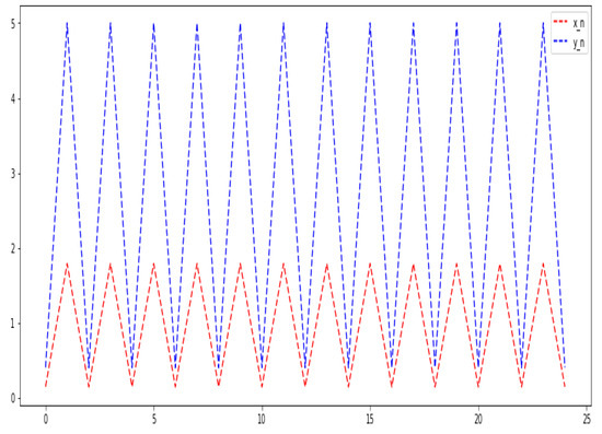
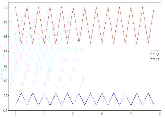
For illustration, we give numerical examples (see Figure 1 and Figure 2).

Theorem 2.

If $x_0=-x_{-2},y_0=-y_{-2},a=c,b=-d$ and $x_{-1}{y}_{-2}=-x_{-2}{y}_{-1}=\frac{1+a}{b}$, then the solution of the system $x_{n+1}=\frac{x_{n-2}{y}_{n-1}}{y_n(a+b{x}_{n-2}{y}_{n-1})},y_{n+1}=\frac{y_{n-2}{x}_{n-1}}{x_n(c+d{y}_{n-2}{x}_{n-1})}$ is periodic with period four.

Proof. 

Under the given assumptions $x_0=-x_{-2},y_0=-y_{-2},a=c,b=-d$, we have

$$\begin{array}{cc}\hfill x_{4n-2}& =\frac{x_0^n{y}_0^n}{y_{-2}^n{x}_{-2}^{n-1}}{\displaystyle \prod _{s=0}^{n-1}}\frac{a^{2s}+(ab-b)x_{-2}{y}_{-1}{\displaystyle \sum _{l=0}^{s-1}}{a}^{2l}}{a^{2s}+(ab-b)x_{-2}{y}_{-1}{\displaystyle \sum _{l=0}^{s-1}}{a}^{2l}}\frac{a^{2s+1}+\left(-a^{2s}b+(ab-b){\displaystyle \sum _{l=0}^{s-1}}{a}^{2l}\right)y_{-2}{x}_{-1}}{a^{2s+1}+\left(a^{2s}b+(-ab+b){\displaystyle \sum _{l=0}^{s-1}}{\left(ac\right)}^l\right)x_{-1}{y}_0}\hfill \\ \hfill & =\frac{x_0^n{y}_0^n}{y_{-2}^n{x}_{-2}^{n-1}}{\displaystyle \prod _{s=0}^{n-1}}\frac{a^{2s+1}+\left(-a^{2s}b+(ab-b){\displaystyle \sum _{l=0}^{s-1}}{a}^{2l}\right)(-y_0)x_{-1}}{a^{2s+1}+\left(a^{2s}b+(-ab+b){\displaystyle \sum _{l=0}^{s-1}}{\left(ac\right)}^l\right)x_{-1}{y}_0}\hfill \\ \hfill & =x_{-2},\hfill \end{array}$$

(89)

$$\begin{array}{cc}\hfill x_{4n-1}& =\frac{x_{-1}{x}_{-2}^n{y}_{-2}^n}{x_0^n{y}_0^n}{\displaystyle \prod _{s=0}^{n-1}}\left(\frac{{\left(a\right)}^{2s}+(ab-b)x_{-1}{y}_0{\displaystyle \sum _{l=0}^{s-1}}{\left(ac\right)}^l}{a^{2s+1}+\left({\left(a\right)}^{2s}b+(-ab+b){\displaystyle \sum _{l=0}^{s-1}}{\left(a\right)}^{2l}\right)x_{-2}{y}_{-1}}\right.\hfill \\ \hfill & \left.\times \frac{a^{2s+1}+\left(-{\left(a\right)}^{2s}b+(ab-b){\displaystyle \sum _{l=0}^{s-1}}{\left(a\right)}^{2l}\right)x_0{y}_{-1}}{{\left(a\right)}^{2s+2}+(-ab+b)x_{-1}{y}_{-2}{\displaystyle \sum _{l=0}^s}{\left(a\right)}^{2l}}\right)\hfill \\ \hfill & =\frac{x_{-1}{x}_{-2}^n{y}_{-2}^n}{x_0^n{y}_0^n}{\displaystyle \prod _{s=0}^{n-1}}\frac{{\left(a\right)}^{2s}+(ab-b)x_{-1}{y}_0{\displaystyle \sum _{l=0}^{s-1}}{\left(ac\right)}^l}{{\left(a\right)}^{2s+2}+(ab-b)x_{-1}{y}_0{\displaystyle \sum _{l=0}^s}{\left(a\right)}^{2l}}.\hfill \end{array}$$

(90)

However, $x_{-1}{y}_{-2}=\frac{1+a}{b}$, i.e., $x_{-1}{y}_0=-\frac{(1+a)(1-a)}{b(1-a)}$ implies that $(a-1)b{x}_{-1}{y}_0=(1-a)(1+a)$, i.e., $a^2+(ab-b)x_{-1}{y}_0=1$ implying

$$a^{2s+2}+(ab-b)x_{-1}{y}_0{a}^{2s}=a^{2s}$$

so that

$$x_{4n-1}=x_{-1}.$$

$$\begin{array}{cc}\hfill x_{4n}& =\frac{x_0^{n+1}{y}_0^n}{x_{-2}^n{y}_{-2}^n}{\displaystyle \prod _{s=0}^{n-1}}\frac{a^{2s+1}+\left(-a^{2s}b+(ab-b){\displaystyle \sum _{l=0}^{s-1}}{a}^{2l}\right)x_{-1}(-y_0)}{a^{2s+1}+\left(a^{2s}b+(-ab+b){\displaystyle \sum _{l=0}^{s-1}}{a}^{2l}\right)x_{-1}{y}_0}\frac{{\left(a\right)}^{2s+2}+(ab-b)x_{-2}{y}_{-1}{\displaystyle \sum _{l=0}^s}{a}^{2l}}{a^{2s+2}+(-ab+b)x_0{y}_{-1}{\displaystyle \sum _{l=0}^s}{a}^{2l}}\hfill \\ \hfill & =x_0,\hfill \end{array}$$

(91)

$$\begin{array}{cc}\hfill x_{4n+1}& =\frac{x_{-2}^{n+1}{y}_{-2}^n{y}_{-1}}{x_0^n{y}_0^{n+1}(a+b{x}_{-2}{y}_{-1})}{\displaystyle \prod _{s=0}^{n-1}}\left(\frac{a^{2s+1}+\left(-{\left(a\right)}^{2s}b+(ab-b){\displaystyle \sum _{l=0}^{s-1}}{\left(a\right)}^{2l}\right)x_0{y}_{-1}}{{\left(a\right)}^{2s+2}+(-ab+b)x_{-1}{y}_{-2}{\displaystyle \sum _{l=0}^s}{\left(a\right)}^{2l}}\right.\hfill \\ \hfill & \times \left.\frac{{\left(a\right)}^{2s+2}+(ab-b)x_{-1}{y}_0{\displaystyle \sum _{l=0}^s}{\left(a\right)}^{2l}}{a^{2s+3}+\left({\left(a\right)}^{2s+2}b+(-ab+b){\displaystyle \sum _{l=0}^s}{\left(a\right)}^{2l}\right)x_{-2}{y}_{-1}}\right)\hfill \\ \hfill & =\frac{x_{-2}^{n+1}{y}_{-2}^n{y}_{-1}}{x_0^n{y}_0^{n+1}(a+b{x}_{-2}{y}_{-1})}{\displaystyle \prod _{s=0}^{n-1}}\left(\frac{a^{2s+1}+\left({\left(a\right)}^{2s}b+(-ab+b){\displaystyle \sum _{l=0}^{s-1}}{\left(a\right)}^{2l}\right)x_{-2}{y}_{-1}}{a^{2s+3}+\left({\left(a\right)}^{2s+2}b+(-ab+b){\displaystyle \sum _{l=0}^s}{\left(a\right)}^{2l}\right)x_{-2}{y}_{-1}}\right).\hfill \end{array}$$

(92)

However, $-x_{-2}{y}_{-1}=\frac{1+a}{b}$ implies that $a^3+(a^{2}b-ab+b)x_{-2}{y}_{-1}=a+b{x}_{-2}{y}_{-1}$ which yields

$$a^{2s+3}+(a^{2s+2}b+(-ab+b)a^{2s})x_{-2}{y}_{-1}=a^{2s+1}+a^{2s}b{x}_{-2}{y}_{-1}$$

so that

$$x_{4n+1}=x_1.$$

Similarly, one can show that $y_{4n+j}=y_j$ for all $n\ge 0$ and $j\ge -2$. Indeed, the solution under the given assumptions is periodic with period four. □

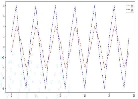
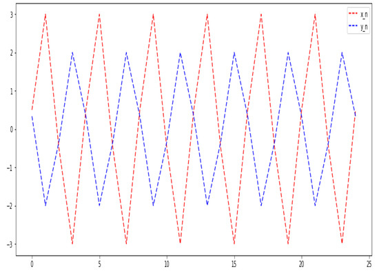
For illustration, we give numerical examples (see Figure 3 and Figure 4).

Remark 1.

If $x_0=-x_{-2},y_0=-y_{-2},a=c=1,d=-1$, then the solution of the system $x_{n+1}=\frac{x_{n-2}{y}_{n-1}}{y_n(a+b{x}_{n-2}{y}_{n-1})},y_{n+1}=\frac{y_{n-2}{x}_{n-1}}{x_n(c+d{y}_{n-2}{x}_{n-1})}$ is periodic with period four. The condition $x_{-1}{y}_{-2}=\frac{1+a}{b}$ is not needed. This is clearly seen from the form of the solution where one replaces $ab-b=0$. This is the case of Theorem 18 of Elsayed [18].

5. Conclusions

We derived the Lie point symmetries of the difference equation (3). The higher-order equations were reduced to lower-order equations, and via iterations, we were able to obtain the solutions of the system of difference equations (2) in an explicit form. The results found in this paper not only generalize the solutions found by Elsayed and Ibrahim in [18] but also greatly simplify the solutions in Theorems 5–12 in the same paper by using only 8 equations instead of 16 equations. It remains an open problem to determine whether or not there are other sufficient conditions for the periodicities in Theorems 1 and 2.

References

- Almatrafi, M.B.; Elsayed, E.M.; Alzahrani, F. The Solution and Dynamic Behavior of Some Difference Equations of Fourth Order. Discret. Impuls. Syst. Ser. Math. Anal. 2022, 29, 33–50. [Google Scholar]
- Almatrafi, M.B. Exact solutions and stability of sixth order difference equations. Electron. J. Math. Anal. Appl. 2022, 10, 209–225. [Google Scholar]
- Almatrafi, M.B.; Alzubaidis, M. The solution and dynamic behaviour of some difference equations of seventh order. J. Appl. Nonlinear Dyn. 2021, 10, 709–719. [Google Scholar] [CrossRef]
- Almatrafi, M.B.; Alzubaidi, M. Stability analysis for a rational difference equation. Arab. J. Basic Appl. Sci. 2020, 27, 114–120. [Google Scholar] [CrossRef]
- Almatrafi, M.B. Analysis of Solutions of Some Discrete Systems of Rational Difference Equations. J. Comput. Anal. Appl. 2021, 29, 355–368. [Google Scholar]
- Almatrafi, M.B.; Alzubaidi, M. Periodic solutions and stability of eight order rational difference equations. J. Math. Comput. Sci. 2022, 26, 405–417. [Google Scholar] [CrossRef]
- Maeda, S. The similarity method for difference equations. IMA J. Appl. Math. 1987, 38, 129–134. [Google Scholar] [CrossRef]
- Ibrahim, T.F.; Khan, A.Q. Forms of solutions for some two-dimensional systems of rational Partial Recursion Equations. Math. Probl. Eng. 2021, 2021, 9966197. [Google Scholar] [CrossRef]
- Ibrahim, T.K. Behavior of Two and Three-Dimensional Systems of Difference Equations in Modelling Competitive Populations. Dyn. Contin. Discret. Impuls. Syst. Ser. 2017, 24, 395–418. [Google Scholar]
- Folly-Gbetoula, M.; Nyirenda, D. Lie Symmetry Analysis and Explicit Formulas for Solutions of some Third-order Difference Equations. Quaest. Math. 2019, 42, 907–917. [Google Scholar] [CrossRef]
- Folly-Gbetoula, M.; Nyirenda, D. On some sixth-order rational recursive sequences. J. Comput. Anal. Appl. 2019, 27, 1057–1069. [Google Scholar]
- Hydon, P.E. Difference Equations by Differential Equation Methods; Cambridge University Press: Cambridge, UK, 2014. [Google Scholar]
- Mnguni, N.; Folly-Gbetoula, M. Invariance analysis of a third-order difference equation with variable coefficients. Dyn. Contin. Discret. Impuls. Syst. Appl. Algorithms 2018, 25, 63–73. [Google Scholar]
- Levi, D.; Vinet, L.; Winternitz, P. Lie group formalism for difference equations. J. Phys. A Math. Gen. 1997, 30, 633–649. [Google Scholar] [CrossRef]
- Folly-Gbetoula, M.; Kara, A.H. Symmetries, conservation laws, and ‘integrability’ of difference equations. Adv. Differ. Equ. 2014, 2014, 224. [Google Scholar] [CrossRef]
- Akbulut, A.; Mirzazadeh, M.; Hashemi, M.S.; Hosseini, K.; Salahshour, S.; Park, C. Triki–Biswas model: Its symmetry reduction, Nucci’s reduction and conservation laws. Int. J. Mod. Phys B 2022, 2022, 2350063. [Google Scholar] [CrossRef]
- Chu, Y.M.; Inc, M.; Hashemi, M.S.; Eshaghi, S. Analytical treatment of regularized Prabhakar fractional differential equations by invariant subspaces. Comput. Appl. Math. 2022, 41, 271. [Google Scholar] [CrossRef]
- Elsayed, E.M.; Ibrahim, T.F. Periodicity and solutions for some systems of nonlinear rational difference equations. Hacet. J. Math. Stat. 2015, 44, 1361–1390. [Google Scholar] [CrossRef]
- Olver, P.J. Applications of Lie Groups to Differential Equations, 2nd ed.; Springer: New York, NY, USA, 1993. [Google Scholar]
- Joshi, N.; Vassiliou, P. The existence of Lie Symmetries for First-Order Analytic Discrete Dynamical Systems. J. Math. Anal. Appl. 1995, 195, 872–887. [Google Scholar] [CrossRef][Green Version]
Publisher’s Note: MDPI stays neutral with regard to jurisdictional claims in published maps and institutional affiliations. |
© 2022 by the authors. Licensee MDPI, Basel, Switzerland. This article is an open access article distributed under the terms and conditions of the Creative Commons Attribution (CC BY) license (https://creativecommons.org/licenses/by/4.0/).