Proton Electromagnetic Form Factors in the Time-like Region through the Scan Technique

Abstract

For over 100 y, scientists have investigated the properties of the proton, which is one of the most abundant components of visible matter in the universe. Nevertheless, researchers do not fully understand many details about its internal structure and dynamics. Time-like electromagnetic form factors are some of the observable quantities that can help us achieve a deeper understanding. In this review article, we present an overview of the current experimental status in this field, consisting of measurements of the time-like reactions $e^{+}{e}^{-}\to p\overline{p}$ and $p\overline{p}\to e^{+}{e}^{-}$ and future measurements of $p\overline{p}\to {\mu }^{+}{\mu }^{-}$. The focus is put on recent high-precision results of the reaction $e^{+}{e}^{-}\to p\overline{p}$ that have been obtained after analyzing 688.5 pb${}^{-1}$ of data taken at the BESIII experiment. They are compared to and put into perspective with results from previous measurements in this channel. We discuss the channels $p\overline{p}\to e^{+}{e}^{-}$ and $p\overline{p}\to {\mu }^{+}{\mu }^{-}$ in terms of the few existing, as well as future measurements, which the PANDA experiment will perform. Finally, we review several new theoretical models and phenomenological approaches inspired by the BESIII high-precision results and then discuss their implications for a deeper understanding of the proton’s structure and inner dynamics.

1. Introduction

The proton, along with its partner nucleon, the neutron, makes up more than 99.9% of the visible matter in the universe. The internal structure and dynamics of the proton, which originate from the strong interaction, has therefore been the target of intense investigations over the past 100 y since the discovery of the proton. Despite that, many questions are still not answered satisfactorily, recent examples being the proton radius puzzle, the proton spin crisis, or the origin of the proton mass. A detailed theoretical description of the internal proton structure and its constituents’ dynamics is made difficult by the non-perturbative nature of the underlying theory, quantum chromodynamics (QCD), within the energy regime of the nucleon. Therefore, precise knowledge of one of the most simple observables that parametrize the proton’s structure and dynamics, the electromagnetic (EM) form factors (FFs), is crucial for understanding the proton structure. In turn, these quantities also provide a perfect testing ground for our understanding of QCD.

The discovery of the proton dates back to the earliest investigations of atomic structure. W. Wien and J. J. Thomson identified a positively charged particle with a mass equal to the hydrogen atom when studying streams of ionized gaseous atoms and molecules whose electrons had been stripped. E. Rutherford indicated that the nitrogen under $\alpha$ particle bombardment ejects what appear to be hydrogen nuclei in 1919. Subsequently, in 1920, E. Rutherford accepted the hydrogen nucleus as an elementary particle, denominating its proton. In 1937, O. Stern observed an anomalous magnetic moment of nucleons (${\mu }_p=2.79{\mu }_N$, ${\mu }_n=-1.91{\mu }_N$), where ${\mu }_N=\frac{e\hslash }{2m_{N}c}$ is the nuclear magneton, while theoretically, the magnetic moment of the point-like proton and neutron is ${\mu }_N$ and zero, respectively. Furthermore, this is the most direct evidence that nucleons are not point-like particles [1]. Afterward, R. Hofstadter established an apparatus for discovering nuclei’s internal structure by elastic scattering of electrons and protons (see Figure 1a). In the 1950s, R. Hofstadter investigated the charge distribution in atomic nuclei and the charge and magnetic moment distributions in the proton and neutron. Nuclei were thereby proven not to be homogeneous, but to have internal structures [2,3]. After that, J. I. Friedman, H. W. Kendall, and R. E. Taylor investigated the deep inelastic scattering of electrons on protons and bound neutrons (see also Figure 1a). This research has been of essential significance for the development of the quark model in particle physics [4,5].

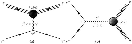
Figure 1. Lowest-order Feynman diagrams for elastic electron–proton scattering $e^{-}p\to e^{-}p$ (a) and for the annihilation process $e^{+}{e}^{-}\to p\overline{p}$ (b).

Until today, the research of the internal structures of protons is one of the hottest topics in nuclear physics. The proton spin crisis and proton radius puzzle are the most critical issues of the research. In 2017, the $\chi$QCD Collaboration reported that the gluon helicity contributes to half of the total proton spin by Lattice QCD [6]. Afterwards, Jefferson Laboratory (PRad) reported a proton radius of $r_p=0.831\pm 0.007\left(\mathrm{stat}\right)\pm 0.012\left(\mathrm{syst}\right)$ [7], which supports the value found by two previous muonic hydrogen experiments [8,9].

Nucleon EM FFs parametrize the difference between a point-like photon-nucleon vertex to one that considers the internal structure of the nucleon. For spin 1/2 particles, such as protons and neutrons, this structure is encoded into two FFs, the Dirac FF ($F_1$) and the Pauli FF ($F_2$), where the first describes the difference from a point-like charge distribution and the second from a point-like magnetization distribution. More commonly used than these Dirac and Pauli FFs are the so-called Sachs FFs $G_E$ and $G_M$, which are simple linear combinations of the former. Proton EM FFs can be explored in two kinematic regions, the spacelike (SL, momentum transfer $q^2<0$) and time-like (TL, momentum transfer $q^2>0$) region. The former region has been extensively investigated through electron–proton scattering experiments (see Figure 1a) since the 1950s, and consequently, proton TL EM FFs are known with low uncertainties of the order of a few percent. Experimental data on the TL region, commonly obtained by investigating annihilation reactions (Figure 1b), has been much more scarce for a long time. Only within the last two decades, more experiments have provided data within this region, and only very recent high-luminosity measurements have brought the precision up to par with the SL region. FFs enter explicitly in the coupling of a virtual photon with the hadron electromagnetic current. Their measurements can be directly compared to hadron models and thereby provide constraints to the description of the internal structure of hadrons [9]. The extension of the proton EM FFs to the TL region opens further possibilities to investigate peculiarities in the structure of the proton. While the information contained in the TL FFs has a less intuitive interpretation compared to the electric and magnetic distribution densities of the nucleon deduced from SL FFs, they play a crucial role in understanding the long-range behavior of strong interactions. Moreover, proton EM FFs can be used to make theoretical predictions for the behavior of other baryons’ FFs, e.g., the neutrons [10].

In terms of $G_E$ and $G_M$, the cross-section of the process $e^{+}{e}^{-}\leftrightarrow p\overline{p}$ reads:

$$\begin{array}{c}\hfill {\sigma }_{e^{+}{e}^{-}\leftrightarrow p\overline{p}}\left(s\right)=\frac{4\pi {\alpha }^2\beta C}{3s}\left[|G_M{\left(s\right)}^2|+\frac{2m_p^2}{s}|G_E{\left(s\right)}^2|\right],\end{array}$$

(1)

where $\alpha$ is the fine structure constant, $\beta =\sqrt{1-4m_p^2/s}$ is the proton velocity, $m_p$ is the proton mass, and C is the Coulomb enhancement factor [11]. From this integrated cross-section, a so-called effective FF ($G_{\mathrm{eff}}$) can be deduced under the assumption of $|G_E\left(s\right)|=|G_M\left(s\right)|$:

$$\begin{array}{c}\hfill |G_{\mathrm{eff}}\left(s\right)|=\sqrt{\frac{{\sigma }_{e^{+}{e}^{-}\leftrightarrow p\overline{p}}\left(s\right)}{\frac{4\pi {\alpha }^2\beta C}{3s}(1+\frac{2m_p^2}{s})}}=\sqrt{\frac{|G_M{\left(s\right)}^2|+\frac{2m_p^2}{s}|G_E{\left(s\right)}^2|}{1+\frac{2m_p^2}{s}}}.\end{array}$$

(2)

This $|G_{\mathrm{eff}}|$ was mainly used by older experiments with limited statistics and was calculated from the measured cross-section using the middle part of the above equation. More recent experiments have been able to perform a measurement of the differential cross-section through an angular analysis in one-photon exchange approximation in the $e^{+}{e}^{-}$ center-of-mass (c.m.) system, which allows determining the individual FFs $|G_E\left(s\right)|$ and $|G_M\left(s\right)|$:

$$\begin{array}{c}\hfill \frac{d{\sigma }_{p\overline{p}}\left(s\right)}{d\Omega }=\frac{{\alpha }^2\beta C}{4s}\left[|G_M{\left(s\right)|}^2(1+{cos}^2\theta )+\frac{4m_p^2}{s}{|G_E\left(s\right)|}^2{sin}^2\theta \right],\end{array}$$

(3)

where $\theta$ is the polar angle of the outgoing particles.

Various approaches to providing a theoretical description of the proton EM FFs exist, among them approaches based on modified versions of the old, yet still relevant, vector meson dominance (VMD) model [12], models based on the unitarity and analyticity of the proton FFs using dispersion theoretical approaches [13], descriptions based on a relativistic constituent quark model [14], and more. A comprehensive review of all these approaches is outside the scope of this article. Instead, the focus is put on a review of the experimental results for the proton TL FFs, especially from the most recent high-luminosity BESIII energy scan and the current, primarily phenomenological theoretical approaches to describe the newly observed features in the effective TL proton FF, as well as the individual electric and magnetic FF.

2. Scan Method

Measuring nucleon EM FFs over a wide kinematical range is possible through two different methods, the so-called initial state radiation (ISR) and scan methods. The ISR method uses collider data at a fixed c.m. energy and analyses events where a photon is emitted from the initial state (see Figure 2a), thus reducing the momentum transfer $q^2$ of the process. This allows measuring FFs at $q^2$ values from the threshold up to the fixed c.m. energy of the collider. For the scan method, this is achieved by taking energy scan data sets, where the c.m. energy of the collider is systematically varied. Within this paper, only former results, as well as future experiments employing the scan method, are reviewed, whereas an overview of results with the ISR method can be found in [15]. Further reviews about nucleon EM FFs in the TL region in general and other baryon FFs can be found in [16] and [17], respectively.

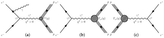
Figure 2. Feynman diagrams for the ISR (a) and Born (b) process of $e^{+}{e}^{-}\to p\overline{p}$, as well as the time-reverse process $p\overline{p}\to e^{+}{e}^{-}$ (c).

3. Overview of Time-like Electromagnetic Form Factor Measurements for the Proton

3.1. Previous Measurements of the Proton EM FFs

Previous measurements of the proton EM FFs using the scan method have been performed with the processes $e^{+}{e}^{-}\to p\overline{p}$, as well as the time-reverse process, $p\overline{p}\to e^{+}{e}^{-}$ (see Figure 2b,c). While processes where muons replace the electron and positron are possible, no FF measurements have been performed employing these channels yet. So far, such measurements were infeasible either due to a lack of ${\mu }^{+}{\mu }^{-}$ colliders or, in the time-reversed case, due to a combination of low statistics and high background contamination, and the same is true for tauons. Proposals for measurements in the muon channel will be discussed in the next section.

The earliest attempts to measure proton EM FFs in the time-like region were performed in the 1970s, in the case of electron–positron annihilation at the ADONE collider in Frascati [18] and in the case of $p\overline{p}$ annihilation reactions with the Proton Synchrotron (PS) at CERN [19]. In the 1980s and 1990s, measurements of electron–positron annihilation were continued at these facilities with the FENICE experiment [20,21,22] at ADONE, as well as the DM1 [23] and DM2 [24,25] experiments at the Orsay colliding beam facility (DCI) in Orsay. FENICE measured at five energy scan points between 1.90 GeV and 2.44 GeV with a total integrated luminosity (${\mathcal{L}}_{\mathrm{int}}$) of 0.36 pb${}^{-1}$, whereas DM1 and its successor DM2 both performed scans with an integrated luminosity of about 0.4 pb${}^{-1}$ between 1.925 GeV and 2.226 GeV in four and six energy steps, respectively. The time-reversed channel was further explored with the PS170 [26,27,28] experiment, using the $\overline{p}$ beam available at the Low Energy Antiproton Ring (LEAR) at CERN, in a series of scan measurements performed between 1991 and 1994 with momentum transfer from the proton–antiproton production threshold up to 2.05 GeV. Additional measurements using this reaction at higher momentum transfer were also performed at the E760 [29] and E835 [30,31] experiments at Fermilab, in the case of E760 in three steps between 2.98 GeV and 3.6 GeV (${\mathcal{L}}_{\mathrm{int}}=26.5$ pb${}^{-1}$) and in the case of E835 in a total of ten steps between 2.97 GeV and 4.29 GeV (${\mathcal{L}}_{\mathrm{int}}=194.5$ pb${}^{-1}$). In the 2000s, the first high-precision, high-luminosity measurements started in the electron–positron channel in the form of an extended energy scan between 2.00 GeV and 3.07 GeV performed with the Beijing Spectrometer (BES) at the Beijing Electron–Positron Collider (BEPC) [32], as well as a single high-luminosity scan point at 3.671 GeV obtained with the CLEO-c detector at the Cornell Electron Storage Ring (CESR) [33]. The CMD-3 experiment at the VEPP-2000 $e^{+}{e}^{-}$ collider performed a fine energy scan of the proton TL EM FFs between the threshold and 2 GeV, divided into 10 energy points in 2016 and an additional 11 energy points in 2019 [34,35]. Finally, the most recent and by far most precise results for the proton time-like EM FFs obtained with the energy scan technique stem from a new high-luminosity scan measurement performed in 2015 [36] and 2020 [37] with the BESIII detector at BEPCII. This new data comprise 22 energy scan points between 2.00 GeV and 3.08 GeV, with a total integrated luminosity of 688.5 pb${}^{-1}$. The high luminosity of this new data allows a precise determination of the individual FFs $|G_E|$ and $|G_M|$, as well as their ratio R, whereas most previous experiments have been limited to the determination of $|G_{\mathrm{eff}}|$.

3.2. Future Experimental Prospects

Further measurements of the proton TL EM FFs are necessary to confirm the results obtained by the newest BESIII measurement for the individual FFs $|G_E|$ and $|G_M|$, as well as their ratio. In addition, more data are necessary to investigate newly found structures that appear both in the effective and the individual FFs. An extension of the measured kinematical range for the separate FFs, both towards higher c.m. energies and the threshold region, is also desirable.

For proton TL EM FF measurements with the scan technique, the most promising upcoming experiment is the PANDA experiment currently under construction at the Facility for Antiproton and Ion Research (FAIR) in Darmstadt. Located at the High-Energy Storage Ring (HESR), which will provide a $\overline{p}$ beam with luminosities up to ${10}^{32}$ cm⁻²s⁻¹ and momenta between 1.5 GeV/c and 15 GeV/c, the PANDA detector will be divided into a target spectrometer and a forward spectrometer. A detailed description of the detector can be found in [38].

Proposals for proton TL EM FF measurements exist both for the channel $p\overline{p}\to e^{+}{e}^{-}$, as well as $p\overline{p}\to {\mu }^{+}{\mu }^{-}$. Measurements, especially of the individual proton TL EM FFs employing the first channel, will be of high interest since they are the only existing. Rather, an old measurement by PS170 is in disagreement with newer $e^{+}{e}^{-}\to p\overline{p}$ results both from the scan and ISR method. The second channel will be the first access to proton TL EM FFs using leptons other than electrons, which will also allow for tests of lepton universality. Feasibility studies exist for both channels: for the electron channel [39], the expected relative uncertainties range between 1% and 5% for the FF ratio ($|G_E/G_M|$) and 1% and 4% for $|G_E|$ in the already explored $q^2$ range up to 3 GeV/c. The expected uncertainty for both R and $|G_E|$ grows to more than 50% at 3.73 GeV/c. However, this would still be an essential extension of the kinematical range of the measurement of the individual FFs. Uncertainties for $|G_M|$ would be well below 1% for all momentum transfers. In the case of the muon channel [40], uncertainties would range between 3% and 27% for $|G_E|$, 2% and 10% for $|G_M|$, and 5% and 37% for the $|G_E/G_M|$ in the energy range between 2.25 GeV and 2.86 GeV.

4. Discussion of Proton TL EM FF Results

Within this section, the different TL EM FF measurements of the experiments introduced in the last section are compared and put into perspective. The comparison starts with the cross-section of the process $e^{+}{e}^{-}\leftrightarrow p\overline{p}$ in Section 4.1, which was determined by most experiments performing scan measurements of proton FFs. While it is not directly a measurement of proton FFs, the cross-section is closely related to the effective FF $|G_{\mathrm{eff}}|$ (see Equation (2)), which is discussed in Section 4.2. Therefore, the discussion in the latter section applies to both the cross-section and $|G_{\mathrm{eff}}|$. Finally, the measurements of the FF ratio, as well as the individual electric ($|G_E|$) and magnetic ($|G_E|$) proton FFs are compared in Section 4.3 and Section 4.4, respectively.

4.1. Measurements of the Cross-Section of $e^{+}{e}^{-}\leftrightarrow p\overline{p}$

Measurements of the cross-section of $e^{+}{e}^{-}\leftrightarrow p\overline{p}$ from $e^{+}{e}^{-}$ colliders employing the scan technique are summarized in Figure 3a for c.m. energies from the threshold up to 2.35 GeV and in Figure 3b for c.m. energies between 2.35 GeV and 4.00 GeV.

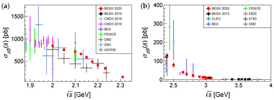
Figure 3. Comparison of the results for the $e^{+}{e}^{-}\leftrightarrow p\overline{p}$ cross-section using the energy scan strategy in (a) $2m_p<\sqrt{s}<2.35$ GeV and (b) $2.35<\sqrt{s}<4.00$ GeV. Shown are the published measurements from BESIII [36,37], CMD3 [34,35], CLEO [33], BES [32], FENICE [20,21,22], E835 [30,31], E760 [29], DM2 [24,25], DM1 [23], and ADONE [18].

4.2. Measurements of the Effective FF $|G_{eff}|$ of the Proton

Measurements of the proton EM FFs of most previous experiments in the TL region were restricted to measuring $|G_{\mathrm{eff}}|$, as shown in Equation (2), due to limited statistics. Instead of the assumption of $|G_E|=|G_M|$, some experiments at high values of $q^2$ (e.g., E760 and E835) also measured the magnetic FF $|G_M|$ under the assumption that the $|G_E|$ contribution is negligible at high energies due to the suppression by a factor of $1/\tau$ (see Equation (3)), with $\tau =\frac{s}{4m_p^2}$.

A comparison of $|G_{\mathrm{eff}}|$ of the proton determined by the different experiments is shown in Figure 4a for c.m. energies from the threshold up to 2.35 GeV and in Figure 4b for c.m. energies between 2.35 GeV and 4.00 GeV. Within their respective uncertainties, the measurements agree well with each other. Measurements close to the threshold, especially by the PS170 experiment, show a steep rise of $|G_{\mathrm{eff}}|$ towards the threshold, while data at higher momentum transfer mostly follow a dipole behavior. A deviation from this behavior can only be seen in the most precise measurement recently performed at BESIII, where a periodic behavior was found to be superimposed over the monotonous decrease of $|G_{\mathrm{eff}}|$. The origin of this structure is still under debate, with possible sources being rescattering of the forming final state particles or intermediate resonance states before the formation of the proton–antiproton state, which enhances the cross-section of the process within a certain momentum transfer region. A more detailed discussion of this phenomenon can be found in Section 5.3.

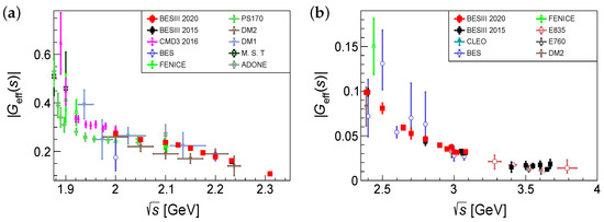
Figure 4. Comparison of the results for $|G_{\mathrm{eff}}|$ using the energy scan strategy in (a) $2m_p<\sqrt{s}<2.35$ GeV and (b) $2.35<\sqrt{s}<4.00$ GeV. Shown are all the published measurements from BESIII [36,37], CMD3 [34,35], CLEO [33], BES [32], FENICE [20,21,22], E835 [30,31], E760 [29], PS170 [26,27,28], DM2 [24,25], DM1 [23], M.S.T [19], and ADONE [18].

4.3. Measurements of the FF Ratio $|G_E/G_M|$ of the Proton

Measurements with the scan technique of the individual proton TL EM FFs over a wider momentum transfer range are limited to three published measurements, two of which were performed with the BESIII detector. A determination of the ratio of the electric and magnetic FF requires an angular analysis of the data, while a separate measurement of $|G_E|$ and $|G_M|$ additionally requires precise knowledge of the luminosity of the acquired data. For most proton TL EM FF measurements, either this knowledge was missing or the amount of detected events did not allow for a measurement of the differential cross-section.

In one-photon approximation, the FFs $|G_E|$ and $|G_M|$, or equivalently their ratio $|G_E/G_M|$ and $|G_M|$, can be determined from a fit to the proton angular distribution for energy points with a sufficiently high number of selected candidates. The range of the angular analysis in most experiments is limited to $cos\theta$ from $-0.8$ to $0.8$. The formula used to fit the proton angular distribution, deduced from Equation (3), can be expressed as:

$$\begin{array}{c}\hfill \begin{array}{c}\hfill \frac{dN}{ϵ\left(1+\delta \right)\times dcos\theta }=\frac{{\mathcal{L}}_{\mathrm{int}}\pi {\alpha }^2\beta C}{2s}{|G_M|}^2\left[\left(1+{cos}^2\theta \right)+\frac{4m_p^2}{s}{\left|\frac{G_E}{G_M}\right|}^2\left(1-{cos}^2\theta \right)\right],\end{array}\end{array}$$

(4)

where $ϵ(cos\theta )$ is the angular-dependent efficiency, including both the detector efficiency and the efficiency from the event selection, and $(1+\delta )(cos\theta )$ is the correction factor for both radiative corrections, such as ISR and final state radiation (FSR), as well as vacuum polarization effects. Both correction factors were obtained from Monte Carlo (MC) simulation. After applying the corrections, the $|cos\theta |$ distribution is fit with Equation (4). An example of the angular distribution of outgoing protons including such a fit is shown in Figure 5 at 2.125 GeV and 2.396 GeV from the most recent BESIII measurement [37].

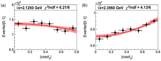
Figure 5. Fit to the $|cos\theta |$ distributions at (a) 2.125 GeV and (b) 2.396 GeV at BESIII [37], after the application of angular-dependent $ϵ(1+\delta )$ factors.

The published results for the existing measurements of the $|G_E/G_M|$ using the scan technique are shown in Figure 6. The most recent BESIII results are the most extensive and precise ones. They agree well with the previous BESIII results obtained with smaller statistics. The single measurement point from CMD3 is also in good agreement within its uncertainties. In contrast, the PS170 results show a systematic trend towards smaller values of $|G_E/G_M|$, which is not confirmed by the BESIII results.

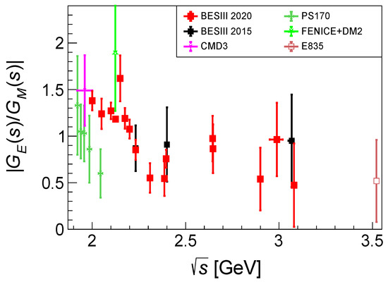
Figure 6. Comparison of the results for $|G_E/G_M|$ using the energy scan strategy. Shown are all the published measurements from BESIII [36,37], CMD3 [34,35], PS170 [26,27,28], FENICE+DM2 [20,21,22,24,25,41], and E835 [30,31,41].

4.4. Measurements of the $|G_E|$ and $|G_M|$ of the Proton

In the case of $|G_E|$, the only published results are from the recent BESIII high-luminosity scan measurement. However, both the smaller, previous BESIII scan, as well as PS170 measured $|G_E/G_M|$ and $|G_M|$, which would allow for the calculation of $|G_E|$. The sole direct measurement of $|G_E|$ is shown on the left side of Figure 7a, while the right side (b) shows a comparison of the results for $|G_M|$.

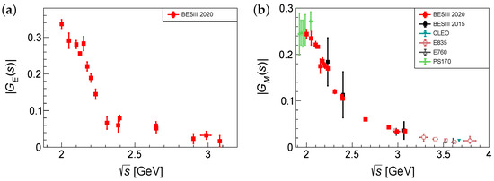
Figure 7. Comparison of the results for (a) $|G_M|$ and (b) $|G_E|$ using the energy scan strategy. Shown are all the published measurements from BESIII [36,37], CLEO [33], E835 [30,31], E760 [29], and PS170 [26,27,28].

For $|G_M|$, the available measurements are all in agreement, albeit the BESIII measurement from 2020 is by far the most precise. It should be noted that the three measurements at high momentum transfer by CLEO, E780, and E835 were performed under the assumption of $|G_E|=0$ instead of extraction through angular analysis. Therefore, they are more of an $|G_{\mathrm{eff}}|$, albeit the assumption may be justified due to the strong suppression of $|G_E|$ at higher energies.

Both $|G_E/G_M|$, as well as the individual FF measurement, especially that of $|G_E|$, seem to show a periodic structure on top of a dipole-like, monotonously falling behavior. This structure is similar to the one already observed in $|G_{\mathrm{eff}}|$; however, in the case of the individual FFs, it is only visible for the high-precision fine-scan data from 2020. The first approaches to describe these features have been made from the theoretical side with mostly phenomenological approaches. However, more investigations, especially concerning the origin of these structures, are necessary. From the experimental side, independent confirmation of the BESIII measurement of $|G_E/G_M|$, $|G_E|$, and $|G_M|$ is needed to confirm this behavior. An attempt at a phenomenological description of these structures can be found in Section 5.4.

5. Theoretical Approaches to the Description of Time-like Electromagnetic Proton Form Factors

5.1. Test of Perturbative QCD and Low-Energy Effective Theory for QCD

The recently obtained high-precision results in the TL region provide information to improve our understanding of the proton’s inner structure and test theoretical models that depend on perturbative QCD (pQCD) and low-energy effective theory for QCD (low-energy-eff-QCD). The low energy region is the regime of low-energy-eff-QCD due to the growing of the running QCD coupling constant and the associated confinement of quarks and gluons. The energy region between 2.00 GeV and 3.08 GeV connects the low-energy-eff-QCD and the pQCD regime. Therefore, Reference [37] suggested a fit function for the energy dependence of ${\sigma }_{p\overline{p}}$ within this energy region, consisting of a low-energy-eff-QCD and a pQCD part:

$$\begin{array}{c}\hfill {\sigma }_{p\overline{p}}\left(s\right)=\left\{\begin{array}{c}\hfill \begin{array}{cc}\hfill {\sigma }_{\mathrm{eff}-\mathrm{QCD}}\left(s\right)& =\frac{e^{a_c}{\pi }^2{\alpha }^3}{s\left[1-e^{-\frac{\pi {\alpha }_s\left(s\right)}{\beta \left(s\right)}}\right]\left[1+{\left(\frac{\sqrt{s}-2m_p{c}^2}{a_0}\right)}^{a_1}\right]},\sqrt{s}\le 2.3094\mathrm{GeV},\hfill \end{array}\\ \hfill \begin{array}{cc}\hfill {\sigma }_{\mathrm{pQCD}}\left(s\right)& =\frac{2\pi {\alpha }^2\beta \left(s\right)C\left[2+{\left(\frac{2m_p{c}^2}{\sqrt{s}}\right)}^2\right]e^{2a_2}}{3s^5{\left[4{ln}^2\left(\frac{\sqrt{s}}{a_0}\right)+{\pi }^2\right]}^2},\sqrt{s}>2.3094\mathrm{GeV},\hfill \end{array}\end{array}\right.\end{array}$$

(5)

with the strong coupling constant ${\alpha }_s\left(s\right)$ and the fine-structure constant $\alpha$. For the strong coupling constant, the following parametrization is used:

$$\begin{array}{cc}\hfill {\alpha }_s\left(s\right)& ={\left[\frac{1}{{\alpha }_s\left(m_Z^2{c}^4\right)}+\frac{25}{12\pi }ln\left(\frac{s}{m_Z^2{c}^4}\right)\right]}^{-1},\end{array}$$

(6)

with the mass of the Z boson $m_Z=91.1876$ GeV/$c^2$ and the strong coupling constant at the Z pole ${\alpha }_s\left(m_Z^2{c}^4\right)=0.11856$. Instead of introducing the Coulomb enhancement factor, the suggested fit function in [37] (Equation 5) uses an alternative approach close to the $p\overline{p}$ threshold by considering gluon exchange between the $B\overline{B}$ pair. In addition, the first part of Equation (5) describes the behavior near the threshold by considering strong interaction effects from the low-energy-eff-QCD for the low-energy region near the $p\overline{p}$ threshold [42,43]. The second part of the formula describes the pQCD behavior of the cross-section, computed in leading order for the continuum region at high momentum transfer [44].

In conclusion, the low-energy-eff-QCD-based description is suitable for the lower-energy behavior below 2.3094 GeV, while the pQCD-based approach provides a good description for the cross-section data at higher energy, which is illustrated in Figure 8. The results and meaning of the fit parameters are as follows: $a_0=332\pm 3$ MeV is the overall QCD parameter; $a_1=4.78\pm 0.13$ is the ${\sigma }_{p\overline{p}}\left(s\right)$ power-law dependence, which is related to the number of valence quarks; $a_2=4.39\pm 0.01$ is a normalization constant. Finally, $a_c$ makes ${\sigma }_{\mathrm{low}\text{-}\mathrm{energy}\text{-}\mathrm{eff}\text{-}\mathrm{QCD}}\left(2.3094\mathrm{GeV}\right)={\sigma }_{\mathrm{pQCD}}\left(2.3094\mathrm{GeV}\right)$ and does not attend to the global fit.

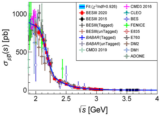
Figure 8. Summary of the $e^{+}{e}^{-}\leftrightarrow p\overline{p}$ cross-section and a fit to the data (blue solid line and band) according to Equation (5). The shown data are the published measurements from BESIII [36,37,45,46], BABAR [47,48,49], CMD3 [34,35], CLEO [33], BES [32], FENICE [20,21,22], E835 [30,31], E760 [29], DM2 [24,25], DM1 [23], and ADONE [18]. In the fit, ${\chi }^2$ is defined as ${\chi }^2={\sum }_i{[f\left(x_i\right)-y_i]}^2/{\mathrm{err}}_i^2$, where ${\mathrm{err}}_i$ is the error of the measured results including statistical and correlated systematic uncertainties, f is the fit function, and n.d.f. is the number of degrees of freedom.

5.2. Possible Resonance Structures in the $p\overline{p}$ System

A description of the cross-section of $e^{+}{e}^{-}\leftrightarrow p\overline{p}$ according to a pQCD and low-energy-eff-QCD model was introduced in Section 5.1. The slight ridges and bump structures occurring here imply that the model in Section 5.1 and its description of the low-energy-eff-QCD and pQCD regime are not perfect. Various approaches have been proposed to describe these deviations, including resonance structures [50] and periodic interference structures [44]. In the first instance, possible resonance structures are considered as convex modifications to the overall concave function describing $|G_{\mathrm{eff}}|$ at invariant masses of around 2.00–2.25 GeV. The approach will be introduced in the following, and the fit parameters are extracted with improved precision by including the new high-luminosity data from BESIII. The line shape of $|G_{\mathrm{eff}}|$ is fit using a coherent sum of a Breit–Wigner function and a nonresonant term [50]:

$$\begin{array}{c}\hfill {\sigma }_{e^{+}{e}^{-}\leftrightarrow p\overline{p}}\left(s\right)=\frac{4\pi {\alpha }^2\beta C}{3s}\left(1+\frac{2m_p^2}{s}\right){|G_{\mathrm{eff}}^{\mathrm{n}.\mathrm{r}.}+A_{p\overline{p}}^{\mathrm{Res}\left(2150\right)}|}^2.\end{array}$$

(7)

The first term $G_{\mathrm{eff}}^{\mathrm{n}.\mathrm{r}.}$ is the nonresonant contribution,

$$\begin{array}{c}\hfill G_{\mathrm{eff}}^{\mathrm{n}.\mathrm{r}.}=\sqrt{\frac{3s{\sigma }_{p\overline{p}}\left(s\right)}{4\pi {\alpha }^2\beta C(1+\frac{2m_p^2}{s})}},\end{array}$$

(8)

where ${\sigma }_{p\overline{p}}\left(s\right)$ is from Equation (5). The second term $A_{p\overline{p}}^{\mathrm{Res}\left(2150\right)}$ is the Breit–Wigner amplitude:

$$\begin{array}{c}\hfill A_{p\overline{p}}^{\mathrm{Res}\left(2150\right)}=\frac{e^{a_3+i{\Psi }_{\mathrm{Res}\left(2150\right)}}}{m_{\mathrm{Res}\left(2150\right)}^2-s-i{\Gamma }_{\mathrm{Res}\left(2150\right)}{m}_{\mathrm{Res}\left(2150\right)}},\end{array}$$

(9)

with normalization factor $a_3$, mass $m_{\mathrm{Res}\left(2150\right)}$, width ${\Gamma }_{\mathrm{Res}\left(2150\right)}$, and relative phase angle to the nonresonant component ${\Psi }_{\mathrm{Res}\left(2150\right)}$. The results of the fit parameters are as follows: $a_0={383}_{-20}^{+19}$ MeV, $a_1=6.{20}_{-0.71}^{+0.87}$, $a_2=4.{43}_{-0.03}^{+0.03}$, $a_3=5.{95}_{-0.63}^{+0.43}$, $m_{\mathrm{Res}\left(2150\right)}={2114}_{-19}^{+14}$ MeV/$c^2$, ${\Gamma }_{\mathrm{Res}\left(2150\right)}={240}_{-49}^{+42}$ MeV and ${\Psi }_{\mathrm{Res}\left(2150\right)}=0.{12}_{-0.22}^{+0.27}$, which is illustrated in Figure 9a. This structure at around 2.15 GeV can be attributed, e.g., to the $\rho \left(2150\right)$ resonance [51].

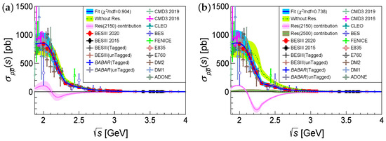
Figure 9. Summary for the $e^{+}{e}^{-}\leftrightarrow p\overline{p}$ cross-section and a fit to the data (blue solid line and band) according to (a) Equation (7) and (b) Equation (10), with the low-energy-eff-QCD and pQCD model (green dashed-dotted curve and band), and contributions from possible resonances at around 2.15 GeV (magenta dotted curve and band) and around 2.5 GeV (teal dashed curve and band). The data shown are the published measurements from BESIII [36,37,45,46], BABAR [47,48,49], CMD3 [34,35], CLEO [33], BES [32], FENICE [20,21,22], E835 [30,31], E760 [29], DM2 [24,25], DM1 [23], and ADONE [18]. The definition of ${\chi }^2$ is the same as in Figure 8.

An additional resonance at around 2.5 GeV can also be considered in the fit [50]:

$$\begin{array}{c}\hfill {\sigma }_{e^{+}{e}^{-}\leftrightarrow p\overline{p}}\left(s\right)=\frac{4\pi {\alpha }^2\beta C}{3s}\left(1+\frac{2m_p^2}{s}\right){|G_{\mathrm{eff}}^{\mathrm{n}.\mathrm{r}.}+A_{p\overline{p}}^{\mathrm{Res}\left(2150\right)}+A_{p\overline{p}}^{\mathrm{Res}\left(2500\right)}|}^2,\end{array}$$

(10)

where $A_{p\overline{p}}^{\mathrm{Res}\left(2500\right)}$ is the Breit–Wigner amplitude:

$$\begin{array}{c}\hfill A_{p\overline{p}}^{\mathrm{Res}\left(2500\right)}=\frac{e^{a_4+i{\Psi }_{\mathrm{Res}\left(2500\right)}}}{m_{\mathrm{Res}\left(2500\right)}^2-s-i{\Gamma }_{\mathrm{Res}\left(2500\right)}{m}_{\mathrm{Res}\left(2500\right)}},\end{array}$$

(11)

with normalization factor $a_4$, mass $m_{\mathrm{Res}\left(2500\right)}$, width ${\Gamma }_{\mathrm{Res}\left(2500\right)}$, and relative phase angle to the nonresonant component ${\Psi }_{\mathrm{Res}\left(2500\right)}$. The results of the fit parameters are as follows: $a_0={438}_{-17}^{+14}$ MeV, $a_1=12.{39}_{-2.76}^{+4.58}$, $a_2=4.{59}_{-0.07}^{+0.07}$, $a_3=7.{03}_{-0.38}^{+0.37}$, $m_{\mathrm{Res}\left(2150\right)}={2178}_{-16}^{+20}$ MeV/$c^2$, ${\Gamma }_{\mathrm{Res}\left(2150\right)}={296}_{-47}^{+54}$ MeV, ${\Psi }_{\mathrm{Res}\left(2150\right)}=0.{65}_{-0.12}^{+0.12}$, $a_4=5.{10}_{-0.52}^{+0.52}$, $m_{\mathrm{Res}\left(2500\right)}={2540}_{-68}^{+67}$ MeV/$c^2$, ${\Gamma }_{\mathrm{Res}\left(2500\right)}={238}_{-86}^{+103}$ MeV and ${\Psi }_{\mathrm{Res}\left(2500\right)}=-0.{13}_{-0.74}^{+0.54}$, which is illustrated in Figure 9b. The significance of the two possible resonance structures is determined to be 4.2$\sigma$.

The corresponding work states that this is not a rigorous analysis since these resonance structures overlap and are not separable from the background. Nevertheless, the addition of two resonances peaking at around 2.15 GeV and 2.50 GeV significantly improves the description of the data [50].

5.3. Periodic Interference Structures in the TL Proton FF

The second mentioned approach to describe the periodic structures in $|G_{\mathrm{eff}}|$ is presented in this section. The corresponding variables of the fit are determined with improved precision with the new high-luminosity data from BESIII.

The data of the time-like $|G_{\mathrm{eff}}|$ are best reproduced by the three-pole model function proposed in [52],

$$\begin{array}{c}\hfill F_{3\mathrm{p}}\left(s\right)=\frac{\mathcal{A}}{(1+\frac{s}{m_a^2{c}^4}){[1-\frac{s}{0.71{\mathrm{GeV}}^2}]}^2}.\end{array}$$

(12)

A global fit to all available results for $|G_{\mathrm{eff}}|$ using the above equation was performed and is shown as the green dashed-dotted curve and band in Figure 10a. The residuals between the fit function and the experimental data indicate a periodic structure when they are represented as a function of the relative momentum $p\left(s\right)=\sqrt{s(\frac{s}{4m_p^2}-1)}$ of the $p\overline{p}$ pair [53]. Phenomenologically, the structure can be described by an oscillating function suggested in [53]:

$$\begin{array}{c}\hfill F_{\mathrm{osc}}\left[p\left(s\right)\right]=b_0^{\mathrm{osc}}{e}^{-b_1^{\mathrm{osc}}p\left(s\right)}cos[b_2^{\mathrm{osc}}p\left(s\right)+b_3^{\mathrm{osc}}].\end{array}$$

(13)

The corresponding fit to the residuals is shown as the magenta dotted curve and band in Figure 10a and the magenta solid curve and band in Figure 10b. Additionally, a global fit to $|G_{\mathrm{eff}}|$ using the sum of two contributions [44,54] was performed:

$$\begin{array}{c}\hfill |G_{\mathrm{eff}}\left(s\right)|=F_{3\mathrm{p}}\left(s\right)+F_{\mathrm{osc}}\left[p\left(s\right)\right].\end{array}$$

(14)

Here, $\mathcal{A}=8.{79}_{-0.21}^{+0.22}$, $m_a^2=9.{04}_{-0.58}^{+0.62}$ GeV${}^2/c^4$, $b_0^{\mathrm{osc}}=0.06\pm 0.01$, $b_1^{\mathrm{osc}}=0.93\pm 0.07$ GeV/$c^{-1}$, $b_2^{\mathrm{osc}}=5.{02}_{-0.09}^{+0.10}$ GeV/$c^{-1}$, and $b_3^{\mathrm{osc}}=0.{61}_{-0.16}^{+0.15}$ are obtained from our fit, which is illustrated as the blue solid line and band in Figure 10a.

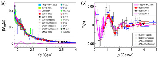
Figure 10. Summary of (a) the effective FF of the proton $|G_{\mathrm{eff}}|$ and a fit to the data (blue solid line and band) according to Equation (14) suggested in [44,54] with the 3-pole (green dashed-dotted curve and band) and oscillation (magenta dotted curve and band) contributions; (b) residuals of the proton $|G_{\mathrm{eff}}|$, after subtraction of the smooth function described by Equation (12), as a function of the relative momentum $p\left(s\right)=\sqrt{s(\frac{s}{4m_p^2}-1)}$ with a fit of the oscillation according to Equation (13) (magenta solid curve and band). The shown data are the published measurements from BESIII [36,37,45,46], BABAR [47,48,49], CMD3 [34,35], CLEO [33], BES [32], FENICE [20,21,22], E835 [30,31], E760 [29], PS170 [26,27,28], DM2 [24,25], DM1 [23], M. S. T [19], and ADONE [18]. The definition of ${\chi }^2$ is the same as in Figure 8.

Periodic interference structures of $|G_{\mathrm{eff}}|$ for the proton manifest as a deviation from a modified dipole behavior. A similar oscillation with a comparable frequency is observed for the neutron, albeit with a significant phase difference, as illustrated in Figure 11. The fit yields $b_2^{\mathrm{osc}}=5.{05}_{-0.09}^{+0.10}$ GeV/$c^{-1}$, the phase of proton, $b_{3\left(p\right)}^{\mathrm{osc}}=0.{57}_{-0.16}^{+0.14}$, $b_{3\left(n\right)}^{\mathrm{osc}}=2.{82}_{-0.21}^{+0.22}$, and a phase difference of $\Delta b_3^{\mathrm{osc}}=|b_{3\left(p\right)}^{\mathrm{osc}}-b_{3\left(n\right)}^{\mathrm{osc}}|={\left({129}_{-10}^{+11}\right)}^{\circ }$. The result indicates unexplored intrinsic dynamics that lead to almost orthogonal oscillations.

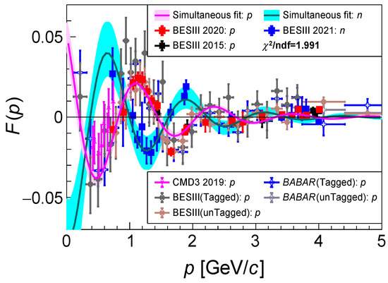
Figure 11. Summary of the residuals of the proton and neutron $|G_{\mathrm{eff}}|$, after subtraction of the smooth function described by Equation (12), as a function of the relative momentum $p\left(s\right)=\sqrt{s(\frac{s}{4m_p^2}-1)}$ with a fit of the oscillation according to Equation (13) (magenta and cyan solid curve and band for the proton and neutron, respectively). The shown data are the published measurements from BESIII (proton [36,37,45,46] and neutron [55]), BABAR [47,48,49], and CMD3 [34,35]. The definition of ${\chi }^2$ is the same as in Figure 8.

5.4. Phenomenological Analysis of $|G_E/G_M|$

Following a similar approach as for $|G_{\mathrm{eff}}|$ in Section 5.3, a fit is performed on the ratio of $|G_E|$ and $|G_M|$ in the TL region, using a function that consists of a damped oscillation on top of a decreasing monopole part [54]:

$$\begin{array}{c}\hfill |\frac{G_E\left[\omega \left(s\right)\right]}{G_M\left[\omega \left(s\right)\right]}|=\frac{1}{1+\frac{\omega {\left(s\right)}^2}{c_0}}\{1+c_1{e}^{-c_2\omega \left(s\right)}sin\left[c_3\omega \left(s\right)\right]\},\end{array}$$

(15)

where $\omega \left(s\right)=\sqrt{s}-2m_p{c}^2$, and the unitary normalization at the production threshold $|\frac{G_E\left[\omega \left(4m_p^2\right)\right]}{G_M\left[\omega \left(4m_p^2\right)\right]}|=1$ is imposed. A fit to the available $|G_E/G_M|$ results returns the parameters $c_0=3.{56}_{-1.47}^{+4.14}$ GeV${}^2$, $c_1=0.{58}_{-0.13}^{+0.21}$, $c_2=2.{17}_{-1.05}^{+1.50}$ GeV${}^{-1}$, and $c_3=9.{48}_{-0.57}^{+0.46}$ GeV${}^{-1}$. The results of the fit are shown in Figure 12 as the blue solid curve and band. The green dashed-dotted curve and its band in the same figure represent the monopole component, the magenta dotted curve, and its band represents the oscillation component (shifted up by 0.5). The red dashed-dotted curve in Figure 12 represents the Kuraev model, another form of monopole model [56]:

$$\begin{array}{c}\hfill |\frac{G_E\left(s\right)}{G_M\left(s\right)}|=\frac{{\mu }_p}{1+\frac{s-4m_p^2{c}^4}{c_4}},\end{array}$$

(16)

where ${\mu }_p$ is the proton anomalous magnetic moment (${\mu }_p=2.79$ in units of Bohr magnetons), $c_4=0.74\pm 0.03$ GeV from the fit. The unitary normalization at the production threshold $|\frac{G_E\left(2m_p\right)}{G_M\left(2m_p\right)}|={\mu }_p$ is imposed.

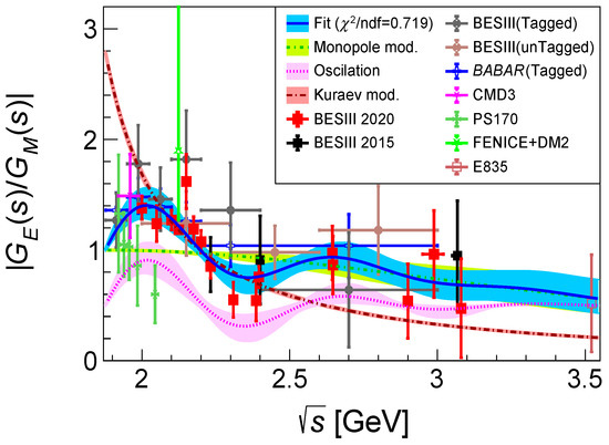
Figure 12. Summary of the ratio $|G_E/G_M|$ of the proton and a fit to the data (blue solid line and band) according to Equation (15) with the monopole (green dashed-dotted curve and band) and oscillation (magenta dotted curve and band) component (shifted up by 0.5), and the Kuraev model [56] (red dashed-dotted curve and band) according to Equation (16). The shown data are the published measurements from BESIII [36,37,45,46], BABAR [47,48,49], CMD3 [34,35], FENICE [20,21,22,41], E835 [30,31,41], PS170 [26,27,28], and DM2 [24,25,41]. The definition of ${\chi }^2$ is the same as in Figure 8.

5.5. Individual FFs $|G_E|$ and $|G_M|$

Using the definition of the effective FF $|G_{\mathrm{eff}}|$ in Equation (2), the electric and magnetic FF can be expressed in terms of $|G_{\mathrm{eff}}|$ and their ratio $|G_E/G_M|$ [54]:

$$\begin{array}{c}\hfill |G_E\left(s\right)|=|G_{\mathrm{eff}}\left(s\right)|\sqrt{\frac{1+\frac{s}{2m_p^2}}{1+\frac{s}{2m_p^2{|\frac{G_E\left(s\right)}{G_M\left(s\right)}|}^2}}},\end{array}$$

(17)

$$\begin{array}{c}\hfill |G_M\left(s\right)|=|G_{\mathrm{eff}}\left(s\right)|\sqrt{\frac{1+\frac{s}{2m_p^2}}{|\frac{G_E\left(s\right)}{G_M\left(s\right)}{|}^2+\frac{s}{2m_p^2}}}.\end{array}$$

(18)

These relations allow calculating $|G_E|$ and $|G_M|$ from the fit results obtained for $|G_E/G_M|$ (Equation (15)) and $|G_{\mathrm{eff}}|$ (Equation (14)) in the previous section. The resulting curves are shown in Figure 13a,b. Here, the blue solid curves and bands represent the fit functions according to Equations (17) and (18), deduced from the fit results of Figure 10 and Figure 12, and the red dashed-dotted curves represent the the Kuraev model [56]:

$$\begin{array}{c}\hfill |G_E\left(s\right)|=\frac{1}{1+\frac{s-4m_p^2{c}^4}{d_0}}\frac{1}{{(1+\frac{s-4m_p^2{c}^4}{d_1})}^2},\end{array}$$

(19)

$$\begin{array}{c}\hfill |G_M\left(s\right)|=\frac{1}{{\mu }_p{(1+\frac{s-4m_p^2{c}^4}{d_2})}^2},\end{array}$$

(20)

where $d_0=0.{41}_{-0.02}^{+0.03}$ GeV${}^2$, $d_1=9.{61}_{-1.87}^{+2.60}$ GeV${}^2$, and $d_2=2.79\pm 0.03$ GeV${}^2$ are obtained from a fit to the available data.

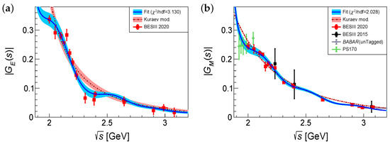
Figure 13. Summary of (a) the electric FF of the proton $|G_E|$ and a fit to the data (blue solid line and band) according to Equation (17) and the Kuraev model [56] Equation (19) (red dashed-dotted line and band); (b) the magnetic FF of the proton $|G_M|$ and a fit to the data (blue solid line and band) according to Equation (18) and the Kuraev model [56] Equation (20) (red dashed-dotted line and band). The shown data are the published measurements from BESIII [36,37,45,46], BABAR [47,48,49], and PS170 [26,27,28]. The definition of ${\chi }^2$ is the same as in Figure 8.

5.6. Theoretical Estimates of the Proton Radius

Precise measurements of FFs in the TL region can also be used to improve the theoretical estimates of the proton radius [44,57]. A direct comparison of the measured TL and space-like (SL) results of the proton EM FF ratio is shown in Figure 14, together with a simple fit according to the model proposed in [56]:

$$\begin{array}{c}\hfill |\frac{G_E\left(s\right)}{G_M\left(s\right)}|=\frac{1}{{\mu }_p(1+\frac{s}{c_0})},\end{array}$$

(21)

where $c_0$ is the same parameter as in Equation (15) and is determined to be $c_0=5.{61}_{-1.33}^{+1.37}$ GeV${}^2$ from the TL-SL joint fit.

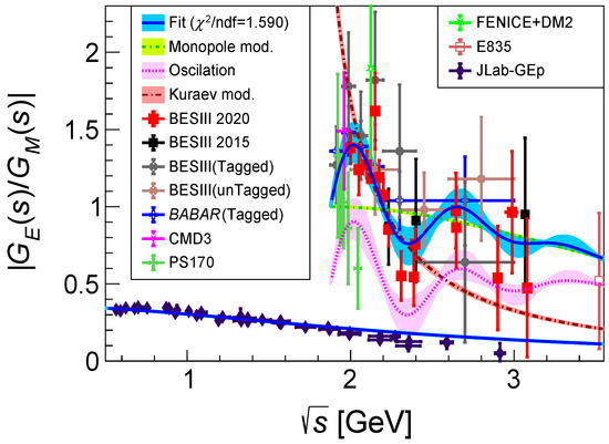
Figure 14. Measured $|G_E/G_M|$ in the time-like region from BESIII [36,37,45,46], BABAR [47,48,49], CMD3 [34,35], BES [32], FENICE+DM2 [20,21,22,24,25,41], E835 [30,31], and PS170 [26,27,28] and in the spacelike region from the GEp Collaboration [58]. The red dashed-dotted line and band are monopole-like fits. The definition of ${\chi }^2$ is the same as in Figure 8.

The model of Equation (21) allows for a prediction of proton EM FFs by connecting annihilation reactions ($l^{+}{l}^{-}\leftrightarrow p\overline{p}$) in the TL region to $ep$ elastic scattering in the SL region. Since there are more data available for SL FFs, they have a larger weight compared to TL FFs. Therefore, more TL experimental data over a wider energy range are highly desirable.

6. Conclusions and Prospect

Within this review, the progress in the determination and understanding of the proton EM FF in the TL region, both from the experimental and the theoretical point of view, was highlighted, on the experimental side focusing on the results obtained with the energy scan technique. The development of the field, from early pioneering experimental works, for example, at Frascati [18,20,21,22], up to the unprecedented accuracy results from the BESIII experiment [36,37], was outlined, and exciting future prospects such as the PANDA experiment at HESR [38] show that the investigation of proton EM FFs is still a hot topic even 100 y after the discovery of the proton.

The first successful investigations of the proton TL EM FFs with the scan technique were conducted by measurements of the total cross-section of $e^{+}{e}^{-}\leftrightarrow p\overline{p}$ at $e^{+}{e}^{-}$ or $p\overline{p}$ colliders (illustrated in Figure 3), which resulted in the determination of an effective FF $|G_{\mathrm{eff}}|$, assuming $|G_E|=|G_M|$ (illustrated in Figure 4). Today, most available measurements only provide this auxiliary quantity, which is extracted under an assumption that does not hold over the whole momentum transfer range. Only recently, experiments have been successful in disentangling the proton EM FFs in the TL region through angular analysis (illustrated in Figure 5), measuring the ratio of the two FFs $|G_E/G_M|$ (illustrated in Figure 6). The high luminosity of the most recent BESIII scan data [37] in addition to a precise knowledge of its integrated luminosity allowed for a breakthrough in the comprehension of the proton through the individual determination of $|G_E|$ and $|G_M|$ (illustrated in Figure 7).

As shown in the theoretical interpretation of the experimental data for the cross-section of the reaction, $e^{+}{e}^{-}\leftrightarrow p\overline{p}$, pQCD and low-energy-eff-QCD were authenticated. An interesting phenomenology, in particular the superposition of small periodic structures on an otherwise smooth dipole parametrization of $|G_{\mathrm{eff}}|$, was discovered. Two different approaches currently under discussion to explain these structures were presented: firstly, the possibility of resonant structures around 2.15 GeV and 2.50 GeV, represented as Breit–Wigner functions on top of the non-resonant pQCD and low-energy-eff-QCD description (illustrated in Figure 9a,b) and, secondly, a description based on an oscillating function superimposed on the smooth dipole parametrization (illustrated in Figure 10a,b). Furthermore, a similar periodic behavior for the neutron was observed (illustrated in Figure 11). Using the oscillation approach, the conjoint frequency with the proton oscillation of $b_2^{\mathrm{osc}}=5.{05}_{-0.09}^{+0.10}$ GeV/$c^{-1}$ was extracted, with a phase difference from the proton case of $\Delta b_3^{\mathrm{osc}}=|b_{3\left(p\right)}^{\mathrm{osc}}-b_{3\left(n\right)}^{\mathrm{osc}}|={\left({129}_{-10}^{+11}\right)}^{\circ }$. Similar to the oscillations of $|G_{\mathrm{eff}}|$, a periodic behavior of the ratio $|G_E/G_M|$ was also observed, which can be extended to $|G_E|$ and $|G_M|$ (illustrated in Figure 12 and Figure 13a,b). The period of these oscillations can be related to subhadronic-scale processes [44,59]. We discussed a faster average decrease in $|G_E|$ and $|G_M|$, following a similar behavior as in the SL region, which is in agreement with the predictions of [56] (illustrated in Figure 12 and Figure 13a,b). Finally, we examined the connection of the TL and SL region by a TL–SL joint fit to improve our comprehension of the radius of the proton (illustrated in Figure 14).

Though much progress has been made to deepen our understanding of the proton structure, most experimental results were reported under the scenario of one-photon approximation. In recent years, the scenario of two-photon exchange (TPE) has been re-discussed, starting from a precise measurement of the $G_E/G_M$ ratio by polarized $ep$ scattering experiments [60,61,62,63]. TPE would manifest in a forward–backward asymmetry in the angular distribution in the TL region. Precise measurements of such an asymmetry at BESIII are ongoing, bringing valuable new insights into the contribution of TPE to the process. The ultimate goal in the field of TL nucleon FFs would be the investigation of the phases between the two complex-valued FFs. Theoretical efforts in this direction have already been carried out and will be further pursued in the near future. Experimentally, a measurement of the phase would require a measurement of the proton polarization perpendicular to the plane of the incoming particles, which could be achieved by including a polarimeter in the experimental setup of a collider experiment.

In summary, the study of the proton EM FFs in the TL region has come a long way. Measurements with the scan strategy have been the working horse of previous experiments, as well as future prospects such as PANDA. Independent confirmation of recent high-precision results, as well as further improvements both on the precision, as well as the measured $q^2$ range will further improve our understanding of the proton’s inner structure and dynamics.

References

- Estermann, I.; Simpson, O.C.; Stern, O. The Magnetic Moment of the Proton. Phys. Rev. 1937, 52, 535. [Google Scholar] [CrossRef]
- Hofstadter, R.; McAllister, R.W. Electron Scattering from the Proton. Phys. Rev. 1955, 98, 217. [Google Scholar] [CrossRef]
- McAllister, R.W.; Hofstadter, R. Elastic Scattering of 188 MeV Electrons from the Proton and the Alpha Particle. Phys. Rev. 1956, 102, 851. [Google Scholar] [CrossRef]
- Bloom, E.D.; Coward, D.H.; DeStaebler, H.; Drees, J.; Miller, G.; Mo, L.W.; Taylor, R.E.; Breidenbach, M.; Friedman, J.I.; Hartmann, G.C.; et al. High-Energy Inelastic e−p Scattering at 6∘ and 10∘. Phys. Rev. Lett. 1969, 23, 930. [Google Scholar] [CrossRef]
- Breidenbach, M.; Friedman, J.I.; Kendall, H.W.; Bloom, E.D.; Coward, D.H.; DeStaebler, H.; Drees, J.; Mo, L.W.; Taylor, R.E. Observed Behavior of Highly Inelastic Electron-Proton Scattering. Phys. Rev. Lett. 1969, 23, 935. [Google Scholar] [CrossRef]
- Yang, Y.B.; Sufian, R.S.; Alexandru, A.; Draper, T.; Glatzmaier, M.J.; Liu, K.-F.; Zhao, Y. (χQCD Collaboration). Glue Spin and Helicity in the Proton from Lattice QCD. Phys. Rev. Lett. 2017, 118, 102001. [Google Scholar] [CrossRef]
- Xiong, W.; Gasparian, A.; Gao, H.; Dutta, D.; Khandaker, M.; Liyanage, N.; Pasyuk, E.; Peng, C.; Bai, X.; Ye, L.; et al. A small proton charge radius from an electron–proton scattering experiment. Nature 2019, 575, 147–150. [Google Scholar] [CrossRef]
- Antognini, A.; Nez, F.; Schuhmann, K.; Amaro, F.D.; Biraben, F.; Cardoso, J.M.R.; Covita, D.S.; Dax, A.; Dhawan, S.; Diepold, M.; et al. Proton structure from the measurement of 2S–2P transition frequencies of muonic hydrogen. Science 2013, 339, 417–420. [Google Scholar] [CrossRef]
- Pohl, R.; Antognini, A.; Nez, F.; Amaro, F.D.; Biraben, F.; Cardoso, J.M.R.; Covita, D.S.; Dax, A.; Dhawan, S.; Fernandes, L.M.P.; et al. The size of the proton. Nature 2010, 466, 213–216. [Google Scholar] [CrossRef]
- Dubničková, A.Z.; Dubnička, S. Prediction of neutron electromagnetic form factors behaviors just by the proton electromagnetic form factors data. Eur. Phys. J. A 2021, 57, 307. [Google Scholar] [CrossRef]
- Baldini, R.; Pacetti, S.; Zallo, A.; Zichichi, A. Unexpected features of e+e−→ and e+e−→ cross-sections near threshold. Eur. Phys. J. A 2009, 39, 315–321. [Google Scholar] [CrossRef]
- Lomon, E.L.; Pacetti, S. Timelike and spacelike electromagnetic form factors of nucleons, a unified description. Phys. Rev. D 2012, 85, 113004. [Google Scholar] [CrossRef]
- Lin, Y.H.; Hammer, H.W.; Meißner, U.-G. Dispersion-theoretical analysis of the electromagnetic form factors of the nucleon: Past, present and future. Eur. Phys. J. A 2021, 57, 255. [Google Scholar] [CrossRef]
- de Melo, J.P.B.C.; Frederico, T.; Pace, E.; Pisano, S.; Salmè, G. Timelike and spacelike nucleon electromagnetic form factors beyond relativistic constituent quark models. Phys. Lett. B 2009, 671, 153–157. [Google Scholar] [CrossRef]
- Lin, D.X.; Dbeyssi, A.; Maas, F.E. Time-Like Proton Form Factors in Initial State Radiation Process. Symmetry 2022, 14, 91. [Google Scholar] [CrossRef]
- Denig, A.; Salmè, G. Nucleon electromagnetic form factors in the time-like region. Prog. Part. Nucl. Phys. 2013, 68, 113–157. [Google Scholar] [CrossRef]
- Huang, G.S.; Ferroli, R.B. Probing the internal structure of baryons. Nat. Sci. Rev. 2021, 8, nwab187. [Google Scholar] [CrossRef]
- Castellano, M.; Di Giugno, G.; Humphrey, J.W.; Sassi Palmieri, E.; Troise, G.; Troya, U.; Vitale, S. (ADONE Collaboration). The reaction e+e−→ at a total energy of 2.1 GeV. Nuovo Cimento 1973, 14, 1–20. [Google Scholar] [CrossRef]
- Bassompierre, G.; Binder, G.; Dalpiaz, P.; Dalpiaz, P.F.; Gissinger, G.; Jacquey, S.; Peroni, C.; Schneegans, M.A.; Tecchio, L. (M. S. T Collaboration). First determination of the proton electromagnetic form factors at the threshold of the time-like region. Phys. Lett. B 1977, 68, 477–479. [Google Scholar] [CrossRef]
- Antonelli, A.; Baldini, R.; Bertani, M.; Biagini, M.E.; Bidoli, V.; Bini, C.; Bressani, T.; Calabrese, R.; Cardarelli, R.; Carlin, R.; et al. (FENICE Collaboration). First measurement of the neutron electromagnetic form factor in the time-like region. Phys. Lett. B 1993, 313, 283–287. [Google Scholar] [CrossRef]
- Antonelli, A.; Baldini, R.; Bertani, M.; Biagini, M.E.; Bidoli, V.; Bini, C.; Bressani, T.; Calabrese, R.; Cardarelli, R.; Carlin, R.; et al. (FENICE Collaboration). Measurement of the electromagnetic form factor of the proton in the time-like region. Phys. Lett. B 1994, 334, 431–434. [Google Scholar] [CrossRef]
- Antonelli, A.; Baldini, R.; Benasi, P.; Bertani, M.; Biagini, M.E.; Bidoli, V.; Bini, C.; Bressani, T.; Calabrese, R.; Cardarelli, R.; et al. (FENICE Collaboration). The first measurement of the neutron electromagnetic form factors in the time-like region. Nucl. Phys. B 1998, 517, 3–35. [Google Scholar] [CrossRef]
- Delcourt, B.; Derado, I.; Bertrand, J.L.; Bisello, D.; Bizot, J.C.; Buon, J.; Cordier, A.; Eschstruth, P.; Fayard, L.; Jeanjean, J.; et al. (DM1 Collaboration). Study of the reaction e+e−→ in the total energy range 1925–2180 MeV. Phys. Lett. B 1979, 86, 395–398. [Google Scholar] [CrossRef]
- Bisello, D.; Limentani, S.; Nigro, M.; Pescara, L.; Posocco, M.; Sartori, P.; Augustin, J.E.; Busetto, G.; Cosme, G.; Couchot, F.; et al. (DM2 Collaboration). A measurement of e+e−→ for (1975 ≤ ≤ 2250) MeV. Nucl. Phys. B 1983, 224, 379–395. [Google Scholar] [CrossRef]
- Bisello, D.; Busetto, G.; Castro, A.; Nigro, M.; Pescara, L.; Posocco, M.; Sartori, P.; Stanco, L.; Antonelli, A.; Biagini, M.E.; et al. (DM2 Collaboration). Baryon pairs production in e+e− annihilation at = 2.4 GeV. Z. Phys. C 1990, 48, 23–28. [Google Scholar]
- Bardin, G.; Burgun, G.; Calabrese, R.; Capon, G.; Carlin, R.; Dalpiaz, P.; Dalpiaz, P.F.; de Brion, J.P.; Derre, J.; Dosselli, U.; et al. (PS170 Collaboration). Measurement of the proton electromagnetic form factor near threshold in the time-like region. Phys. Lett. B 1991, 255, 149–154. [Google Scholar] [CrossRef]
- Bardin, G.; Burgun, G.; Calabrese, R.; Capon, G.; Carlin, R.; Dalpiaz, P.; Dalpiaz, P.F.; Derre, J.; Dosselli, U.; Duclos, J.; et al. (PS170 Collaboration). Precise determination of the electromagnetic form factor of the proton in the time-like region up to s = 4.2 GeV2. Phys. Lett. B 1991, 257, 514–518. [Google Scholar] [CrossRef]
- Bardin, G.; Burgun, G.; Calabrese, R.; Capon, G.; Carlin, R.; Dalpiaz, P.; Dalpiaz, P.F.; Derre, J.; Dosselli, U.; Duclos, J.; et al. (PS170 Collaboration). Determination of the electric and magnetic form factors of the proton in the time-like region. Nucl. Phys. B 1994, 411, 3–32. [Google Scholar] [CrossRef]
- Armstrong, T.A.; Bettoni, D.; Bharadwaj, V.; Biino, C.; Borreani, G.; Broemmelsiek, D.; Buzzo, A.; Calabrese, R.; Ceccucci, A.; Cester, R.; et al. (E760 Collaboration). Proton electromagnetic form factors in the time-like region from 8.9 to 13.0 GeV2. Phys. Rev. Lett. 1993, 70, 1212. [Google Scholar] [CrossRef]
- Ambrogiani, M.; Bagnasco, S.; Baldini, W.; Bettoni, D.; Borreani, G.; Buzzo, A.; Calabrese, R.; Cester, R.; Dalpiaz, P.; Fan, X.; et al. (E835 Collaboration). Measurements of the magnetic form factor of the proton in the time-like region at large momentum transfer. Phys. Rev. D 1999, 60, 032002. [Google Scholar] [CrossRef]
- Andreotti, M.; Bagnasco, S.; Baldini, W.; Bettoni, D.; Borreani, G.; Buzzo, A.; Calabrese, R.; Cester, R.; Cibinetto, G.; Dalpiaz, P.; et al. (E835 Collaboration). Measurements of the magnetic form factor of the proton for time-like momentum transfers. Phys. Lett. B 2003, 559, 20–25. [Google Scholar] [CrossRef]
- Ablikim, M.; Bai, J.Z.; Ban, Y.; Bian, J.G.; Cai, X.; Chen, H.F.; Chen, H.S.; Chen, H.X.; Chen, J.C.; Chen, J.; et al. (BES Collaboration). Measurement of the cross-section for e+e−→ at center-of-mass energies from 2.00 to 3.07 GeV. Phys. Lett. B 2005, 630, 14–20. [Google Scholar] [CrossRef][Green Version]
- Pedlar, T.K.; Cronin-Hennessy, D.; Gao, K.Y.; Gong, D.T.; Hietala, J.; Kubota, Y.; Klein, T.; Lang, B.W.; Li, S.Z.; Poling, R.; et al. (CLEO Collaboration). Precision Measurements of the Timelike Electromagnetic Form Factors of Pion, Kaon, and Proton. Phys. Rev. Lett. 2005, 95, 261803. [Google Scholar] [CrossRef] [PubMed]
- Akhmetshin, R.R.; Amirkhanov, A.N.; Anisenkov, A.V.; Aulchenko, V.M.; Banzarov, V.S.; Bashtovoy, N.S.; Berkaev, D.E.; Bondar, A.E.; Bragin, A.V.; Eidelman, S.I.; et al. (CMD Collaboration). Study of the process e+e−→ in the c.m. energy range from threshold to 2 GeV with the CMD-3 detector. Phys. Lett. B 2016, 759, 634–640. [Google Scholar] [CrossRef]
- Akhmetshin, R.R.; Amirkhanov, A.N.; Anisenkov, A.V.; Aulchenko, V.M.; Banzarov, V.S.; Bashtovoy, N.S.; Berkaev, D.E.; Bondar, A.E.; Bragin, A.V.; Eidelman, S.I.; et al. (CMD Collaboration). Observation of a fine structure in e+e−→hadrons production at the nucleon-antinucleon threshold. Phys. Lett. B 2019, 794, 64–68. [Google Scholar] [CrossRef]
- Ablikim, M.; Achasov, M.N.; Ai, X.C.; Albayrak, O.; Albrecht, M.; Ambrose, D.J.; Amoroso, A.; An, F.F.; An, Q.; Bai, J.Z.; et al. (BESIII Collaboration). Measurement of the proton form factor by studying e+e−→. Phys. Rev. D 2015, 91, 112004. [Google Scholar] [CrossRef]
- Ablikim, M.; Achasov, M.N.; Adlarson, P.; Ahmed, S.; Albrecht, M.; Alekseev, M.; Amoroso, A.; An, F.F.; An, Q.; Anita, Y.; et al. (BESIII Collaboration). Measurement of Proton Electromagnetic Form Factors in e+e−→ in the Energy Region 2.00-3.08 GeV. Phys. Rev. Lett. 2020, 124, 042001. [Google Scholar] [CrossRef]
- Lutz, M.F.M.; Pire, B.; Scholten, O.; Timmermans, R.; Boucher, J.; Hennino, T.; Kunne, R.; Marchand, D.; Ong, S.; Pouthas, J.; et al. (PANDA Collaboration). Physics Performance Report for PANDA: Strong Interaction Studies with Antiprotons. arXiv 2009, arXiv:0903.3905v1. [Google Scholar]
- Singh, B.; Erni, W.; Krusche, B.; Steinacher, M.; Walford, N.; Liu, B.; Liu, H.; Liu, Z.; Shen, X.; Wang, C.; et al. (PANDA Collaboration). Feasibility studies of time-like proton electromagnetic form factors at ANDA at FAIR. Eur. Phys. J. A 2016, 52, 325. [Google Scholar] [CrossRef]
- Barucca, G.; Davì, F.; Lancioni, G.; Mengucci, P.; Montalto, L.; Natali, P.P.; Paone, N.; Rinaldi, D.; Scalise, L.; Erni, W.; et al. (PANDA Collaboration). Feasibility studies for the measurement of time-like proton electromagnetic form factors from p→μ+μ− at ANDA at FAIR. Eur. Phys. J. A 2021, 57, 30. [Google Scholar] [CrossRef]
- Ferroli, R.B.; Bini, C.; Gauzzi, P.; Mirazita, M.; Negrini, M.; Pacetti, S. A description of the ratio between electric and magnetic proton form factors by using space-like, time-like data and dispersion relations. Eur. Phys. J. C 2006, 46, 421. [Google Scholar]
- Solovtsova, O.P.; Chernichenko, Y.D. Threshold Resummation S Factor in QCD: The Case of Unequal Masses. Phys. Atom. Nucl. 2010, 73, 1612–1621. [Google Scholar] [CrossRef]
- Ferroli, R.B.; Pacetti, S.; Gauzzi, A. No Sommerfeld resummation factor in →e+e−? Eur. Phys. J. A 2012, 48, 33. [Google Scholar] [CrossRef]
- Bianconi, A.; Tomasi-Gustafsson, E. Periodic Interference Structures in the Timelike Proton Form Factor. Phys. Rev. Lett. 2015, 114, 232301. [Google Scholar] [CrossRef]
- Ablikim, M.; Achasov, M.N.; Adlarson, P.; Ahmed, S.; Albrecht, M.; Alekseev, M.; Amoroso, A.; An, F.F.; An, Q.; Bai, Y.; et al. (BESIII Collaboration). Study of the process e+e−→ via initial state radiation at BESIII. Phys. Rev. D 2019, 99, 092002. [Google Scholar] [CrossRef]
- Ablikim, M.; Achasov, M.N.; Adlarson, P.; Ahmed, S.; Albrecht, M.; Aliberti, R.; Amoroso, A.; An, M.R.; An, Q.; Bai, X.H.; et al. (BESIII Collaboration). Measurement of proton electromagnetic form factors in the time-like region using initial state radiation at BESIII. Phys. Lett. B 2021, 817, 136328. [Google Scholar] [CrossRef]
- Aubert, B.; Barate, R.; Boutigny, D.; Couderc, F.; Karyotakis, Y.; Lees, J.P.; Poireau, V.; Tisserand, V.; Zghiche, A.; Grauges, E.; et al. (BABAR Collaboration). Study of e+e−→ using initial state radiation with BABAR. Phys. Rev. D 2006, 73, 012005. [Google Scholar] [CrossRef]
- Lees, J.P.; Poireau, V.; Tisserand, V.; Grauges, E.; Palano, A.; Eigen, G.; Stugu, B.; Brown, D.N.; Kerth, L.T.; Kolomensky, Y.G.; et al. (BABAR Collaboration). Study of e+e−→ via initial-state radiation at BABAR. Phys. Rev. D 2013, 87, 092005. [Google Scholar] [CrossRef]
- Lees, J.P.; Poireau, V.; Tisserand, V.; Grauges, E.; Palano, A.; Eigen, G.; Stugu, B.; Brown, D.N.; Kerth, L.T.; Kolomensky, Y.G.; et al. (BABAR Collaboration). Measurement of the e+e−→ cross-section in the energy range from 3.0 to 6.5 GeV. Phys. Rev. D 2013, 88, 072009. [Google Scholar] [CrossRef]
- Lorenz, I.T.; Hammer, H.W.; Meißner, U.G. New structures in the proton–antiproton system. Phys. Rev. D 2015, 92, 034018. [Google Scholar] [CrossRef]
- Biagini, M.E.; Dubnicka, S.; Etim, E.; Kolàr, P. Phenomenological evidence for a third radial excitation of ρ (770). Il Nuovo Cimento A 1991, 104, 363–369. [Google Scholar] [CrossRef]
- Tomasi-Gustafsson, E.; Rekalo, M.P. Search for evidence of asymptotic regime of nucleon electromagnetic form factors from a compared analysis in space- and time-like regions. Phys. Lett. B 2001, 504, 291–295. [Google Scholar] [CrossRef]
- Bianconi, A.; Tomasi-Gustafsson, E. Phenomenological analysis of near-threshold periodic modulations of the proton time-like form factor. Phys. Rev. C 2016, 93, 035201. [Google Scholar] [CrossRef]
- Tomasi-Gustafsson, E.; Bianconi, A.; Pacetti, S. New fit of time-like proton electromagnetic form factors from e+e− colliders. Phys. Rev. C 2021, 103, 035203. [Google Scholar] [CrossRef]
- Ablikim, M.; Achasov, M.N.; Adlarson, P.; Ahmed, S.; Albrecht, M.; Aliberti, R.; Amoroso, A.; An, Q.; Lavania, A.; Bai, X.H.; et al. (BESIII Collaboration). Oscillating features in the electromagnetic structure of the neutron. Nat. Phys. 2021, 17, 1200–1204. [Google Scholar]
- Kuraev, E.A.; Dbeyssi, A.; Tomasi-Gustafsson, E. A model for space and time-like proton (neutron) form factors. Phys. Lett. B 2012, 712, 240–244. [Google Scholar] [CrossRef]
- Lorenz, I.T.; Hammer, H.W.; Meißner, U.G. The size of the proton: Closing in on the radius puzzle. Eur. Phys. J. A 2012, 48, 151. [Google Scholar] [CrossRef]
- Puckett, A.J.R.; Brash, E.J.; Jones, M.K.; Luo, W.; Meziane, M.; Pentchev, L.; Perdrisat, C.F.; Punjabi, V.; Wesselmann, F.R.; Afanasev, A.; et al. (GEp Collaboration). Polarization transfer observables in elastic electron–proton scattering at Q2 = 2.5, 5.2, 6.8 and 8.5 GeV2. Phys. Rev. C 2017, 96, 055203, Errutum in Phys. Rev. C 2018, 98, 019907. [Google Scholar] [CrossRef]
- Bianconi, A.; Tomasi-Gustafsson, E. Fourth dimension of the nucleon structure: Spacetime analysis of the time-like electromagnetic proton form factors. Phys. Rev. C 2017, 95, 015204. [Google Scholar] [CrossRef][Green Version]
- Tomasi-Gustafsson, E.; Osipenko, M.; Kuraev, E.A.; Bystritskiy, Y.M. Compilation and analysis of charge asymmetry measurements from electron and positron scattering on nucleon and nuclei. Phys. Atomic. Nucl 2013, 76, 937–946. [Google Scholar] [CrossRef][Green Version]
- Punjabi, V.; Perdrisat, C.F.; Aniol, K.A.; Baker, F.T.; Berthot, J.; Bertin, P.Y.; Bertozzi, W.; Besson, A.; Bimbot, L.; Boeglin, W.U.; et al. (Jefferson Lab Hall A Collaboration). Proton elastic form factor ratios to Q2 = 3.5 GeV2 by polarization transfer. Phys. Rev. C 2005, 71, 055202. [Google Scholar] [CrossRef]
- Gayou, O.; Wijesooriya, K.; Afanasev, A.; Amarian, M.; Aniol, K.; Becher, S.; Benslama, K.; Bimbot, L.; Bosted, P.; Brash, E.; et al. (Jefferson Lab Hall A Collaboration). Measurements of the elastic electromagnetic form factor ratio μpGEp/GMp via polarization transfer. Phys. Rev. C 2001, 64, 038202. [Google Scholar] [CrossRef]
- Gayou, O.; Aniol, K.A.; Averett, T.; Benmokhtar, F.; Bertozzi, W.; Bimbot, L.; Brash, E.J.; Calarco, J.R.; Cavata, C.; Chai, Z.; et al. (Jefferson Lab Hall A Collaboration). Measurement of GEp/GMp in p→e to Q2 = 5.6 GeV/c2. Phys. Rev. Lett. 2002, 88, 092301. [Google Scholar] [CrossRef] [PubMed]
Publisher’s Note: MDPI stays neutral with regard to jurisdictional claims in published maps and institutional affiliations. |
© 2022 by the authors. Licensee MDPI, Basel, Switzerland. This article is an open access article distributed under the terms and conditions of the Creative Commons Attribution (CC BY) license (https://creativecommons.org/licenses/by/4.0/).