
Methodology for Measuring the Cutting Inserts Wear


1
Department of Manufacturing Engineering, Transilvania University of Brasov, B-dul Eroilor 29, 500036 Brasov, Romania
2
SC Siemens Industry Software, B-dul Gării 13A, 500227 Brasov, Romania
*
Author to whom correspondence should be addressed.
Symmetry 2022, 14(3), 469; https://doi.org/10.3390/sym14030469
Submission received: 7 February 2022
/
Revised: 18 February 2022
/
Accepted: 23 February 2022
/
Published: 25 February 2022
(This article belongs to the Special Issue Symmetry in Manufacturing Systems Engineering — Concept and Theory to Improve Design, Process, Quality and Circularity as the Basis for Future Manufacturing Philosophy)
Abstract
:In the industrial manufacturing, the wear of the cutting tool represents the main factor that causes machine downtime and it has a negative influence over the machined surface roughness and dimensional and position deviations. For this reason, the accurate measurement of tool wear both on-line (during machining) and off-line (outside of the machining process) is a necessity. Due to the continuous technology innovation, finding new and more effective methods to measure precisely the wear represents a permanent interest for research. In this paper, after a review of recent developed methods in this field, showing the methods of measuring wear and indicating the error sources when measuring the wear of cutting inserts, the necessity to have a unitary methodology for measuring the flank wear is emphasized. Applying it could obtain the same wear-measured values in the same conditions. For this purpose, the measurement errors are determined, and a new methodology for measuring the cutting insert wear is developed. It was tested in the case of six worn cutting inserts used for the turning process of specimens (1C45 steel), of 50 mm diameter and 300 mm length. By testing the developed methodology, it was found that the errors that can be made by various researchers while measuring wear are acceptable, leading to results that can be considered correct from a practical point of view. In the paper is also presented how the principle of symmetry is used to characterize the wear of the cutting inserts.
Keywords:
asymmetry; cutting process; cutting insert; measurement; symmetry; tool condition monitoring; wear1. Introduction
The current industry is still based on the most common metal cutting processes such as turning, drilling, milling, and grinding due to their performances in precision and quality. The latest research in CAD/CAE/CAPP/CAM systems and modern CNC machines leads to the development of flexible manufacturing systems that are useful for obtaining products at lower prices in medium and even small production systems.
A permanent field of interest for increasing productivity of the flexible manufacturing systems is reducing machine downtime. During machining processes, important time is lost by stopping the process in order to change or restore the cutting tool. The main factor that leads to the process interruption is the wear of the cutting edge. The criteria used to determine the right moment to stop the machining process is the cutting tool life, which represents the effective cutting time until the appearance of the admissible wear.
The importance of a correct determination of the tool life is also supported by the fact that the quality of the final products is directly influenced by the state of the cutting edge in terms of surface roughness, dimensional and shape deviations [1], and cutting with an excessive worn tool can lead to burns and scratches on the machined surface and has a negative influence on the stability of the machining process.
Knowing these facts, it can be stated that the wear of the cutting tools affects the machining process in terms of quality and cost, and this justifies the necessity of new research into wear assessment.
In the literature the methods for tool condition monitoring are synthesized [2], but because there are recent studies in this direction, and this field presents a permanent interest for the industry, their synthesizing in this paper came as a necessity.
From the studied literature it was found that a unitary methodology for measuring the wear of the cutting edge had to be developed so that the results of the measurements could be compared between different researchers. Large measurement errors occur especially when the edge wear is uneven (asymmetrical).
As a consequence, a methodology is proposed and argued with experimental data, and a quantitative analysis of possible human errors is made, when repeatedly measuring the wear, by the same operator, using the same instrument.
A new method is also developed and presented, based on the principles of symmetry, to characterize the flank wear.
2. State of the Art
2.1. The Wear of Cutting Tools and Tool Life
The wear represents the phenomenon of material removal from the active surfaces of the tool during the cutting process and the main causes that lead to its appearance are presented in Figure 1. Zhu et al. [2] present, in their research, a more detailed description of tool wear mechanism. In addition, Xu et al. [3] discovered in their research that the wear due to oxidation, adhesion and diffusion appear mainly on the rake face and the adhesive and diffusion wear appear on the flank face.
According to [4], the cutting tool wear is classified into four main types: the corner wear, the flank wear, the notch wear and the crater wear. The first three types appear on the clearance surface at the contact between the cutting tool and workpiece and the crater wear appears on the rake surface at the contact between tool and chip.
The greatest interest is presented for the flank wear because it appears on every cutting edge of every type of cutting tool and it represents the criteria used for tool life determination.
The flank wear characteristics are described, in accordance with reference [4], in Figure 2 [5], where the worn part of the cutting edge is divided into three main areas: C area—the corner wear, B area—the flank wear, and N area—the notch wear. The cutting tool life is determined by the two main wear parameters: VBMAX—the maximum width and VBB—the average width. These characteristics are measured in the B area. The recommended values for the admissible wear are VBB = 0.3 mm for a regular, uniform wear and VBMAX = 0.6 mm for an irregular wear [1].
Regarding to the crater wear, which can appear together or concomitant with the flank wear, the characteristics are presented, according to [4], in Figure 3 [5], and described as follows: KT—crater depth, KM—distance between the cutting edge and the deepest crater point, KB—distance between the cutting edge and the back crater contour, KF—width of the land between the crater and the cutting edge, KE—radial displacement of the tool corner.
Tool wear evolution in time is marked by three phases [3]: phase I—the break-in, phase II—the normal wear until the admissible wear is reached, phase III—the accelerated wear that can lead to tool fracture. At the end of phase II, the machining process must be stopped, and the cutting edge must be replaced or restored by sharpening. For this reason, to estimate correctly the moment of reaching the admissible wear value, Tool Condition Monitoring (TCM) represents a permanent field of interest.
2.2. Cutting Tool Wear Measurement Methods
Depending on its purpose, the wear measurement can be undertaken on-line, directly on the machine-tool during the cutting process, or off-line, separately of the machine-tool, using the measurement and control instruments.
The on-line method of wear determination is commonly known as the tool condition monitoring technique and, can be classified into direct TCM and indirect TCM. Direct TCM consists in measuring the wear itself with the cutting edge still on the machine-tool, using optical systems, and indirect TCM refers to wear estimation during the machining process, based on measuring other factors correlated with the wear value.
Wear assessment using direct TCM is clearly more accurate than the indirect estimation, but it has some disadvantages. The main disadvantage is represented by the fact that it is still difficult to precisely measure the wear without interrupting the cutting process, thus the machining operation should be stopped for the wear to be measured using vision systems, with the cutting edge still on the machine-tool. Other disadvantages consist of the fact that the cutting edge must be cleaned of chips or cutting fluid, and that the illumination inside the machine-tool is improper.
Indirect TCM relies on sensors that are sensitive to the parameters of the cutting process such as the cutting force, acoustic emission, spindle power, vibration, temperature, and analyzes them in order to evaluate the wear state of the cutting edge and appreciate the moment when it reaches the admissible value, when tool replacement is necessary.
When establishing an indirect TCM method for wear measurement it is necessary to take into consideration all the factors that influence its appearance and development: cutting parameters, material of the workpiece and material of the cutting edge, geometry of the cutting tool and cutting fluids.
Based on these factors used as entry parameters, the machining process outputs signals such as cutting forces, acoustic emission, cutting sound, vibrations, spindle power and current, and temperature, that are acquired and analyzed by TCM systems in order to estimate the wear state of the cutting tool.
In Figure 4 are synthesized the actual methods that are used for cutting tools wear assessment.
For the industrial environment, the research conducted in the TCM field is very important because it is still difficult to find a method that fulfils all the requirements regarding accuracy, reaction speed, productivity, as well as user friendly and low cost. The optical off-line methods for wear assessment are suitable in the research conducted especially for cutting tools manufacturers.
In the research conducted by Attanasio et al. [6], a model for simulation of wear based on FEM on turning was developed. Experimental tests were also performed to validate the results of the EMF and both similarities and discrepancies were found. Haddag and Nouari [7] used FEM to estimate tool wear in turning modeling, and the strength and temperature of the input parameters were measured directly from the cutting process. Binder et al. [8], in the simulation of FEM wear on turning, also used complex coated cutting tools and calibrated the coating model. Pimenov and Guzeev [9] used FEM as an indirect method for wear estimation, simulating the stress conditions at the flank surface and obtaining an intensity equation for the flank wear, for face milling process. The obtained mathematical model can be applied to calculate cutting forces and the flank wear value.
Shi et al. [10] proposed a new method for cutting tool wear simulation and prediction based on the combination between dynamic nodes movement technology and wear rate model. The model was validated by experimental tries at turning with uncoated carbide tool.
2.2.1. On-Line Methods
Direct Tool Condition Monitoring
Measuring the wear during the machining process represents a challenge for the researchers. Due to the cutting fluid, chips and improper illumination, achieving accurate values for wear width could be difficult, and if it is wanted to obtain a wear assessment without interrupting the process, this operation becomes more difficult, but possible due to the continuous development of computer vision and image processing technology.
A very important aspect for obtaining accurate values for the wear is represented by the illumination system. There are several types of illumination systems such as fluorescent or halogen lamps, LED lights, laser or flashlights, and the use of infrared band filters is recommended for obtaining a clearer wear profile [11]. After the flank wear image is captured, image processing techniques are used for improving the clarity of the wear image by noise reduction, for separating the worn surface from the unworn surface and for obtaining the wear contour in order to determine its characteristics.
Currently, machine vision technologies are mostly used for on-machine measurements. Using a Charge-Coupled Device (CCD) camera a system based on successive image analysis for periodic measurement of flank wear [12] in the case of milling operation was developed; images of the worn flank were captured without stopping the spindle, but for low spindle speed.
Zhang developed an algorithm using machine vision for direct wear measurement for ball-end milling cutters, with very accurate results, that involved programming the tool to stop in the same position and cleaning the tool for the measurements [13]. A similar method was developed by Li et al. [14] for cutting inserts, and it was integrated with the CNC machining center.
Other research [15] was proposed for micro-milling, a new region growing method for processing images of the tool wear, based on morphological component analysis. In addition, for monitoring the state of a micro-milling tool is developed a machine vision system using two CCD cameras [16].
Li and An [17] proposed a method for an automatic focusing and segmentation of the worn surface in order to obtain precise values of the flank wear, during turning operation.
To overcome the cutting fluid layer problem in direct TCM method using machine vision, the confocal fluorescence microscopy system is proposed, using a confocal microscope, a CCD camera and a diode laser to induce fluorescence [18].
Regarding the crater wear, its deepness characteristics can be evaluated with additional equipment such as a microscope or a fringe projector that makes 3D data obtaining possible. For this purpose, a tool measurement system is developed [19] and a clamping device for on-machine application using 2D profile laser displacement Keyance. D’Addona et al. deal with both flank and crater wear by interrupting the turning process from minute to minute to capture the image of the flank wear and to measure the crater wear with a microscope to train an artificial neural network and DNA—based computing for wear prediction [20].
Regarding the grinding process, an on-line method for the grinding wheel is presented using a 3D scanning system, based on the analysis of geometrical changes of the flat surfaces. The grinding wheel is scanned on the machine, the method implies the process interruption [21].
Indirect Tool Condition Monitoring
A TCM system consists of both hardware and software and, according to [3], the hardware is used for the signal acquisition and the software for the signal processing and uses artificial intelligence techniques for decision making. Figure 5 presents the indirect TCM system and centralizes information from literature [2,11,22].
- a.
- Cutting force
Cutting force is known to be extremely sensitive to the evolution of tool wear. An increasing wear is sensed by increasing cutting forces, especially tangential and feed force. For the force signal acquisition there are used dynamometers and strain gauges. Two strain gauges mounted on the tool holder were used to detect the changes in both feed force (Fx) and tangential force (Fz), and a statistical signal processing method was used to correlate the input parameters with the wear value [23]. In Ref. [3], for the force signal acquisition during milling process, a dynamometer placed under the workpiece and for feature extraction was used for the time—frequency domain. A method for tool wear monitoring in the case of the milling process was developed [24]. It tracks four cutting force coefficients that seemed to be independent of the cutting conditions, but still correlated with the state of the cutting tool.
A prediction program based on cutting forces during turning with ceramic tools is presented in Ref. [25]. It predicts total tool wear and the wear due to different wear mechanisms. Other mathematical models for wear prediction based on the cutting force were identified in Refs. [26,27,28,29]; in their research the authors of Ref. [30] the cutting force as well as the wear images obtained with a microscope or machine vision system.
Neural networks were used for decision making when the input signal was represented by the cutting forces by research for milling [31]. The authors of Refs. [32,33] used a neuro-fuzzy model to predict wear during the turning process and cutting force as monitoring signal, and introduced the Levenberg–Marquardt algorithm to train an auto-associative neural network to evaluate the wear status during the milling process [34]. Gao et al. [35] introduced for tool wear state monitoring during turning, using a Hidden Markov tree for the statistical processing of cutting force. The latest research uses different signals, concomitant, to monitor the cutting process. For example, for the milling process Ref. [36] uses cutting forces, as well as vibration and acoustic emission to develop a prediction method using support vector regression. The same input parameters but during the turning process were used by Karam et al. [37] to train a neural network decision making algorithm regarding wear monitoring. For the drilling process are used, as input parameters, the cutting force, torque, chip thickness and the wear values obtained with a microscope, and the authors proposed a co-evolutionary particle swarm optimization-based selective neural network ensembles enabled tool wear prediction model [38]. It was demonstrated that the model is more effective than the conventional single neural network model.
- b.
- Vibration
The cutting forces, under the influence of many factors, become inconstant in time, a fact that leads to the vibration appearance. This phenomenon leads to an improper quality of the machined surface and to a faster wear evolution or even to cutting tool failure.
Research as in Ref. [39] presented the influence of the cutting tool wear on the vibration, and the experiments conducted by Fang et al. [40] showed that vibrations increase while wear evolves. The experiments presented in Ref. [41] showed that when a certain critical vibrational intensity is exceeded, the wear of the cutting tool is dramatically increased.
The sensors used for vibration signal acquisition are accelerometers. In Ref. [42] these were used to measure the vibration signals from the workpiece of a Laser Doppler Vibrometer, during turning operation.
Rmili et al. developed an automatic detector for tool wear state, in case of turning process, using vibration signal. The extracted feature from the acquisitioned signal was mean power and it was demonstrated that this parameter is relevant for wear description [43]. The k-star algorithm was used to classify the extracted features from vibrational signal during turning, based on the entropy [44].
Aghdam et al. modeled the vibration signals using autoregressive moving average models in order to obtain the relation between them and the flank wear [45], and Ref. [46] used, besides vibration signals, force and acoustic emission to train a back propagation neural network in order to estimate the remaining useful life of the cutting tool during the milling process.
For de-noising the vibration signal and feature extraction, Kilundu et al. [47] combined singular spectrum analysis and band-pass filtering, and the obtained results recommend using data mining techniques for tool condition monitoring.
Cutting tool life estimation methods are also approached in the woodworking industry where the influence of cutting vibration on tool wear during milling process was studied using an industrial robot [48].
- c.
- Acoustic emission and cutting sound
The acoustic emission can be defined, according to Refs. [11,49], as a spontaneous energy release due to a local change in the material microstructure. The acoustic emission signal is collected using microphones or thin film piezoelectric sensors. For the signal acquisition, the sensors should be placed as close as possible to the cutting site, but some limitations exist, such as the cutting fluids or chips that will cover them, or such as other ambient sounds that will interfere with the cutting sound. If these limitations are overcome, acoustic emission signal can successfully detect wear evolution.
For tool wear monitoring using acoustic emission, to correlate the signal with the tool wear, the Power-Spectral Density and auto-covariance techniques are used [49]. Bhuiyan et al. conducted an experiment replicating the cutting insert wear by grinding process, where the workpiece is represented by the cutting insert, and the cutting tool is the grinding wheel [50].
Kulandaivelu et al. separated the flank wear and the crater wear for tool condition monitoring and correlated each one with the emitted acoustic signals [51]. During their experimental tries, the correlation between the acoustic emission and the flank wear was realized by placing the piezoelectric sensor on the side surface of the tool holder and the correlation with the crater wear, by placing the sensor on the top surface of the tool holder. Zafar et al. in Ref. [52] used neural networks for noise filtration in the acoustic signal during the turning process. Other research that used acoustic emission signals for tool condition monitoring were also conducted [53,54].
Ren et al. [55] proposed a tool condition monitoring system based on type-2 fuzzy modeling of the acoustic emission signal, during turning process. Li et al. [56] predicted tool wear using logistic regression models and wavelet analysis for signal processing and feature extraction. The conducted experiments for milling led to the conclusion that acoustic emission together with cutting forces can better predict the wear state. In this direction, both acoustic emission and cutting force resulted from the turning process for tool condition monitoring are used [57,58].
Another signal lately used in tool wear monitoring is the cutting sound. The experiments conducted by Besmir and Kim [59] during the end-milling process, led to the result that the cutting sound recorded by the microphone could successfully detect the wear evolution change, from the stable wear phase to the accelerated wear phase. Seemuang et al. recorded the sound emitted during turning with a microphone and filtered the unwanted noise. The results showed that, between the frequency of spindle noise and tool wear there exists no link, but the magnitude of spindle noise frequency spectrum andits cumulative value can be used for wear monitoring [60]. Zhang et al. conducted the experiments using both acoustic emission and cutting sound for tool wear monitoring and found that they complement each other, a fact that makes this monitoring technique better than using only one of them [61].
- d.
- Motor current and spindle power
Several research targeted the correlation between the cutting force and the motor current signal of the machine-tool. The results showed that the cutting forces can be successfully estimated by measuring the motor current signal, and used this correlation for tool wear monitoring during machining processes. Nouri Khajavi et al. used, in their research, feed motor current, spindle speed, cutting feed and cutting depth as input parameters for a neural network to predict the wear state of the cutting tool during the milling process [62].
Another monitored signal used for wear assessment during cutting processes is the power consumption. Ref. [63] is presented how the mean power consumption for every minute during turning and developed correlations with the wear evolution is recorded
Even though this method represents a simple, low-cost wear monitoring technique without interfering with the machining process, it is less sensitive to the wear evolution than the monitoring the cutting forces method [1].
- e.
- Machined surface roughness
The surface roughness of the machined workpiece represents a parameter which is directly affected by the tool wear. The machined surface roughness can be monitored using machine vision, profilometers and surface roughness analyzers [1], or for obtaining an on-line 3D analysis of the surface texture, a laser holographic interferometer can be used [64].
The latest research has focused on developing new and effective methods for feature extraction from the machined surface texture images and correlating them with the wear evolution. Research presented in Ref. [65] used gray level co-occurrence method and run-length statistical techniques for milled surface texture analysis, with the result that the grey level non-uniformity and contrast features were well correlated with the tool wear.
Regarding surfaces obtained using the turning process, in research [66], texture analysis using Gray-Level Co-occurrence Matrix (GLCM) technique was used, with the result that the contrast and homogeneity texture descriptors are well correlated with the state of the cutting tool. Other relevant features for tool wear monitoring were extracted using the discrete wavelet transform technique [67]. In research conducted by Dutta et al. [68] for turning, GLCM, Voronoi tessellation and discrete wavelet transform techniques in order were used to extract eight texture descriptors that predicted the wear evolution well. A prediction model was developed using support vector machine model, based on regression analysis, and an on-line wear classification was developed based on the turned surface texture analysis [69].
- f.
- Other methods for indirect wear monitoring
The first studied parameter outputted from the cutting process that is directly connected to the wear of the cutting tool is the temperature in the cutting zone. The temperature significantly affects the wear evolution by accelerating it, and its on-line measurement becomes a necessity. In some research the correlation between the temperature and the tool wear during turning process is investigated [70] and the methods for measuring temperature are synthesized, including thermocouple technique, thin film sensor technique, infrared radiation and infrared thermography [71]. The most used method for temperature measurement is represented by the thermocouples that can be embedded in tools or the workpiece [72].
Directly connected to the temperature, another studied parameter is the electric current at cutting. During metal cutting processes with good electricity conductor edges, at the contact between tool and workpiece appears an electrical current, due mainly to the released heat. Ref. [73] presents a review of the electrical current during machining processes, including the connection with the wear of the cutting tool, and Ref. [74] investigated the influence of the electrical current on the cutting tool life. The electrical current can be measured using digital multimeters or data loggers.
Another parameter used for tool condition monitoring is represented by the displacement of the tool edge. The displacement takes place due to the flank wear, during turning [1]. In Ref. [1] several methods for displacement monitoring are centralized, such as optoelectronic sensors or a nozzle and a pressure medium. Research conducted by Ratava et al. [75] estimates the displacement during interrupted cutting, using an acceleration sensor and use the acquisition signal for tool condition monitoring.
2.2.2. Off-Line Methods
Off-line methods imply measuring the wear of the cutting tool outside the machining process, in laboratory conditions, for very accurate results.
The optical method is the most used for off-line wear assessment and the basic instrument for this measurement is the microscope. Mandal et al. [76] used a stereo microscope for measuring flank wear.
The most accurate results for wear assessment are obtained using Scanning Electron Microscope (SEM), this method being widely used [77]. In research both optical microscope and SEM are used to measure the cutting tool wear characteristics [78,79,80].
Other research in this field is focused on finding new methods for off-line wear assessment and one of them is represented by Reverse Engineering technique. In their research, Valerga et al. [81], after completely modeling the cutting tools, observed that the wear detail appears in the new obtained physical models too, but did not measure it. Ref. [82] presented how this technique for wear measurement is used by digitizing the cutting insert with a laser scanner and developing the CAD model. The results were validated by comparing them with the ones obtained by a stereo microscope.
2.3. Conclusions Regarding Literature Review
Due to continuous technological innovation, finding new and more effective ways to measure wear precisely is of permanent interest. It can be observed that both on-line and off-line methods for wear measurement present a great point of interest for researchers. Regarding on-line direct methods, the trend is focused on using new vision technology more precisely to capture the wear image during the cutting process, with the development of new efficient methods for image processing and feature extraction. Another approached field in latest research is represented by developing decision-making algorithms based on the captured wear images. A certain future trend in on-line direct measurement of the wear is developing technologies and techniques for wear assessment during the cutting process, without interrupting it.
Regarding on-line indirect methods, the latest research is not focused on finding new parameters that are correlated with the wear or with developing new sensors because the ones which have been used up until now are still considered adequate for tool condition monitoring. The research is more orientated on developing mathematical models [83,84,85], on finding the best methods to process the acquisitioned signal and methods of extracting features that precisely determine the wear evolution, and on decision making algorithms [86,87,88]. A trend for future research is the development of self-powering, wireless sensor technologies for tool condition monitoring [89].
Regarding off-line methods, the accuracy of the results obtained for wear measurement depend on more factors, some of them being the measurement instrument, the conditions in which the measurement was performed and also the experience of the operator in appreciating the transition from the worn surface to the unworn surface. Since the human factor also has an influence on the final result, a unitary methodology for measuring the wear comes as a necessity, in order to minimize the measurement errors and to obtain comparable results between researchers.
Research concerning tool condition monitoring must be carried on to find accurate, user friendly, low cost and flexible methods that can be applied in the industrial environment to increase productivity by reducing machine downtime.
3. Materials and Methods
The materials and means that were used are presented in research [5]. There were used six carbide cutting inserts SPMR150612, P type, produced by Carmesin Bucharest, Romania, and from each insert one cutting edge was used for turning. The front clearance angle was 5°, the back rake angle was 6° and the side cutting edge angle was 45°. The turning process was performed on a universal lathe SNB400 produced by Aris Arad, Romania, without cooling, and it was used as a specimen of Ø50 and 300 mm length, from C45(1.0503) steel, supplied by Antera steel Targoviste, Romania, material which has the following chemical composition, in accordance to [90]: C = 0.45%, Si = 0.22%, Mn = 0.56%, P = 0.025%, S = 0.034. The tensile strength of C45(1.0503) steel is 660 MPa and the hardness is 224 HB.
At the beginning, a first specimen was made from a bar of Ø50 mm at which the surface layer was removed by cutting, and the final diameter measured with a classic micrometer was Ø42.19 mm; with the lathe rotational speed of n = 800 rev/min, the actual cutting speed (Table 1) was calculated and it was used for turning with all the inserts. For further use of the specimen, the rotational speed was increased to n = 1000 rev/min and in order to keep the same value for the cutting speed, the diameter of the specimen was brought to the value of Ø27 mm, and a new turning was performed with the insert to be worn. In this way, on a specimen it was turned 3 times at the same cutting speed; the effective cutting times for a specimen were calculated and the adopted tool life of 10 min was divided by the cutting time of a specimen, resulting in 3 cutting cycles on a specimen to wear an edge.
The used cutting parameters for each edge, used in the research, can be seen in Table 1 [5]. The values for the depth-of-cut were randomly chosen between 2 ÷ 4 mm. Different values were chosen for the depth-of-cut to obtain different lengths of worn edge in order to determine the number of points at which to measure the flank wear. It was considered that the cutting speed and the feed rate did not affect the length of the worn edge and consequently remained constant, a unique value to obtaining the cutting edge wear.
The wear measurements were performed using the Mitutoyo microscope shown in Figure 6. The measurement range of the microscope is 0–50 mm, the digital step of the microscope micrometer is 0.001 µm and the maximum permissible error is ±3 µm [91,92]. The uncertainty of measurement is not indicated precisely for this type of microscope, but for similar microscopes is given by the relation [93]: uncertainty (X,Y) = (2.5 + 0.02 L) µm, where L is the length to be measured. If it is calculated with the length of the longest worn cutting edge (almost 8 mm) it will result an uncertainty of 2.66 µm.
The method for measuring the wear was microscopic visualization and identification of the wear height with an increment of 0.1 mm, the viewing direction being perpendicular to the flank wear. For this purpose, it was necessary to tilt the surface on which the cutting insert lies (Figure 6).
4. Results and Discussions
With the cutting inserts it was turned up to a maximum flank wear of 0.6 ÷ 0.7 mm. The images of the obtained wear can be seen in Figure 7, Figure 8, Figure 9, Figure 10, Figure 11 and Figure 12 [5].
Analyzing Figure 7, Figure 8, Figure 9, Figure 10, Figure 11 and Figure 12, the wear of cutting insert 1 (Figure 7) has the greatest non-uniformity and consequently is most difficult to measure.
The optimization of the measurement increment was presented in research [89], the optimal value being 0.1 mm.
To identify the length of the rectilinear worn edge, in order to determine the number of points at which wear will be measured, the scheme from Figure 13 is used.
For cutting insert 1, the length of the rectilinear worn edge is Lx = 2.705 mm and the real cutting depth is ap = 2.264 mm, even if the lathe setting was at 2.25 mm.
Based on Figure 13 the rectilinear portion of the cutting edge wear was determined without entering the area of the nose radius (r = 1.2 mm) of the cutting plate. At the beginning using the microscope, the M dimension between the end of the wear and the tangent to the radius r (for the squared inserts the tangent is identical to the secondary edge) is measured. From the value of the dimension M, the value of the radius r is subtracted and results in the length of the rectilinear edge Lx. With the length of the rectilinear edge Lx, the number of points where the wear will be measured are determined with the relation Lx/p + 1, in which p = 0.1 mm is the measurement increment. The first point at which wear will be measured is the end of the worn edge. For example, for insert 1 (Figure 7), Lx = 2.705 mm, so the result of Lx/p + 1 will be 28. This means that the number of points at which wear will be measured will be 28.
The measurement increment was performed in [5], the resultant value being 0.1 mm. The cutting insert 1 was used (Figure 7) because it has the most ununiform wear. On the rectilinear portion of the edge, from the end of wear to the nose of the insert, wear was measured using 12 different increments: 0.025 mm, 0.05 mm, 0.075 mm, 0.1 mm, 0.125 mm, 0.15 mm, 0.175 mm, 0.2 mm, 0.25 mm, 0.3 mm, 0.4 mm and 0.5 mm. The average wear for each increment was determined and the values were compared with the average wear determined for the smallest increment (0.025 mm). It was found that the closest average value of wear to that increment of 0.025 mm was obtained with the increment of 0.1 mm.
4.1. Identify Sources of Human Error When Measuring Wear
In order to develop a unitary methodology, it is necessary to analyze the sources of error when measuring wear, but also the error that can be made when repeating measurements by the same operator or the error that can be made when measuring the same wear by different operators using the same measuring instrument. Human errors in the wear measurement can be made regardless of the form of wear (uniform or uneven wear). The sources of human error are shown in Figure 14 on the wear profile associated with the cutting insert 1 viewed under the Hirox RH-2000 microscope, provided by Global Systems, Brasov, Romania. This microscope was used only for obtaining the 3D image of the cutting insert 1 wear. Hirox RH-2000 allows 2D and 3D measurements, and 3D scanning through a high-resolution video system [95].
The first source of human error in measuring flank wear is the alignment of the horizontal reticle 1 of the microscope with the cutting edge. The error in this case is due to the overlap of the horizontal reticle over the cutting edge, an overlap that determines the reference line against which the flank wear VBB is measured. To determine the overlap error, the horizontal reticle was positioned on the edge of the cutting insert. Twenty repetitions were performed of the positioning of the reticle, and the deviation from the first positioning was determined. The result is centralized in Table 2.
The analysis of the data presented in Table 2 shows that the maximum difference of 0.005 mm is insignificant for wear in the cutting process. Only the reticle of the microscope has a thickness of 1µm. In conclusion, this type of error can be overlooked.
The second source of human error in measuring the flank wear is the positioning of the vertical reticle at the end of the wear, on the right side (Figure 14). The reticle determines the origin from which the incremental measurement begins. In this case, 20 repetitions of the positioning of the reticle were performed and the deviation from the first positioning was determined, the result being presented in Table 3.
Analyzing the data in Table 3, it is found that, this time, the maximum deviation increased to 0.006 µm due to the greater difficulty of positioning the vertical reticle.
The third source of human error in measuring the flank wear (Figure 14) is given by the more difficult assessment of the transition from the worn surface of the flank to the unworn surface. This error occurs when the measurements are performed by different operators, but also when the measurements are repeated by the same operator.
4.2. Determination of Operator-Induced Measurement Error
In order to determine the measurement error induced by the operator, 12 measurements of the same wear were performed (Figure 8—insert 1). The starting point of the measurements were given each time by the same indication of the digital micrometer, this determining the same initial position for the vertical reticle in position 2, and the increment of the measured points was 0.1 mm. Wear was measured at 28 points (the number of points being determined with the data in Section 4). A total of 336 measurements were taken. Figure 15 shows the maximum difference between the 12 measurements at each of the 28 points.
Figure 16 shows the average wear value for the 12 measurements of a single operator. It can be seen that the first set of five measurements give approximately the same average wear but with intervening fatigue of the operator, at repetitions, the difference between the average wear increases. The maximum difference between the average wear is 0.011 mm.
- maximum difference between readings is 0.031 mm at points 6, 13, 22 and 26, which means that at these points it is more difficult to notice the transition from relief face to wear;
- maximum difference between the average wears is 0.0106 mm, which is more than acceptable;
- all repeats indicated maximum wear in point 9.
For both the maximum wear of the cutting edge and for the average wear, the deviation resulting from repetition is insignificant for the cutting process and is therefore acceptable. Only at a deviation of 0.1 mm the cutting process is sensitive.
4.3. Difference between Measurements Made by Independent Operators
To see if there were differences between independent operators when measuring the same wear, on the same microscope, six operators measured, separately, the same wear after a session of training. The basis for comparison was the first measurement of the operator, who measured the same wear 12 times. The graphical representation of the results can be seen in Figure 17.
From Figure 17 it can be concluded:
- maximum difference for the measured wear values by operators is 0.068 mm at point 1, which is understandable, being the first measurement; already when measuring the wear in point 2 the difference was reduced to 0.059 mm and then it returned to normal, the difference being as for the first operator, when 12 repetitions were performed;
- maximum difference between the average wears for the six operators is 0.008 mm, which is more than acceptable;
- repeats indicated maximum wear in point 9;
- the points where the transition appreciation from the unworn surface to the worn surface was made with greater difficulty were, namely, points 1, 2, 6, 10, 19, 22 and 25.
4.4. Methodology for Measuring the Flank Wear
The development of a unitary methodology for measuring the flank wear is necessary so that researchers, from anywhere, can obtain the same values. For irregular wear (Figure 7 and Figure 8), applying the unitary methodology, the differences between operators in determining the average wear should not be greater than 0.008 mm. The sequence of steps in the proposed methodology, when measuring the wear on the microscope, is as follows:
- Step 1. Identify the characteristics of the worn cutting insert, especially the nose radius;
- Step 2. Identify the characteristics of the cutting tool holder, first of all of the front clearance angle when positioning on the machine tool;
- Step 3. Position the insert on the microscope table so that the wear on the flank is visible perpendicularly;
- Step 4. Microscopic measurement of the M dimension to determine the worn rectilinear edge Lx (Figure 13);
- Step 5. Determine the number of points on the rectilinear edge where the wear on the flank will be measured (Section 4), the increment being p = 0.1 mm;
- Step 6. Position the horizontal reticle of the microscope along the unworn edge;
- Step 7. Position the vertical reticle of the microscope at the end of wear so that the measurements are made towards the tip of the cutting tool (in this way the nose radius of the cutting insert is avoided—Figure 14);
- Step 8. Wear measurement at each point identified in step 5;
- Step 9. Identify the maximum flank wear VBMAX;
- Step 10. Calculate of the average wear VBB taking into account the maximum value;
- Step 11. Calculate of the ratio between maximum wear and average wear, a ratio that characterizes the degree of non-uniformity of wear.
The application of the proposed methodology to the six worn cutting inserts (Figure 7, Figure 8, Figure 9, Figure 10, Figure 11 and Figure 12) led to the results from Table 4 and Table 5.
From Table 5 it is easy to see that if the ratio between maximum wear and average wear is between 1.1 and 1.2, wear is uniform (Figure 9, Figure 10, Figure 11 and Figure 12), and if the ratio between maximum wear and average wear is between 1.2 and 1.25, that wear has a pronounced un-uniform character (Figure 7 and Figure 8).
4.5. Applying the Principles of Symmetry to Characterize the Wear
One of the principles of symmetry tells us that the more symmetrical an entity is, the more uniform it is. This principle can also be applied to the wear of the edge of a cutting tool, which completes the characterization of the degree of uniformity of the wear by the ratio between the maximum wear and the average wear.
Wear symmetry can be assessed by dividing the flank wear into two equal parts (Figure 18) and calculating the average wear on each side. The ratio between the two average wears, along with the ratio between maximum wear and average wear characterize the degree of uniformity of wear.
Based on the Figure 18 and the data from the Table 4 and Table 5, the resultant data are presented in Table 6. If the number of points where the wear on the flank is measured is odd, then for the first part it will be taken with one point more than the second part. The reverse can also be undertaken, the deviation from the average wear compared to the first case being a maximum of 0.005 mm.
The data from Table 6 indicate that if the superunit ratio between VBB,I and VBB,II is in the range 1 ÷ 1.25 the wear has a symmetrical character, an aspect that is similar to the conclusion obtained by using the ratio VBMAX/VBB. If the superunit ratio between VBB,I and VBB,II is greater than 1.25 the wear has an asymmetric character.
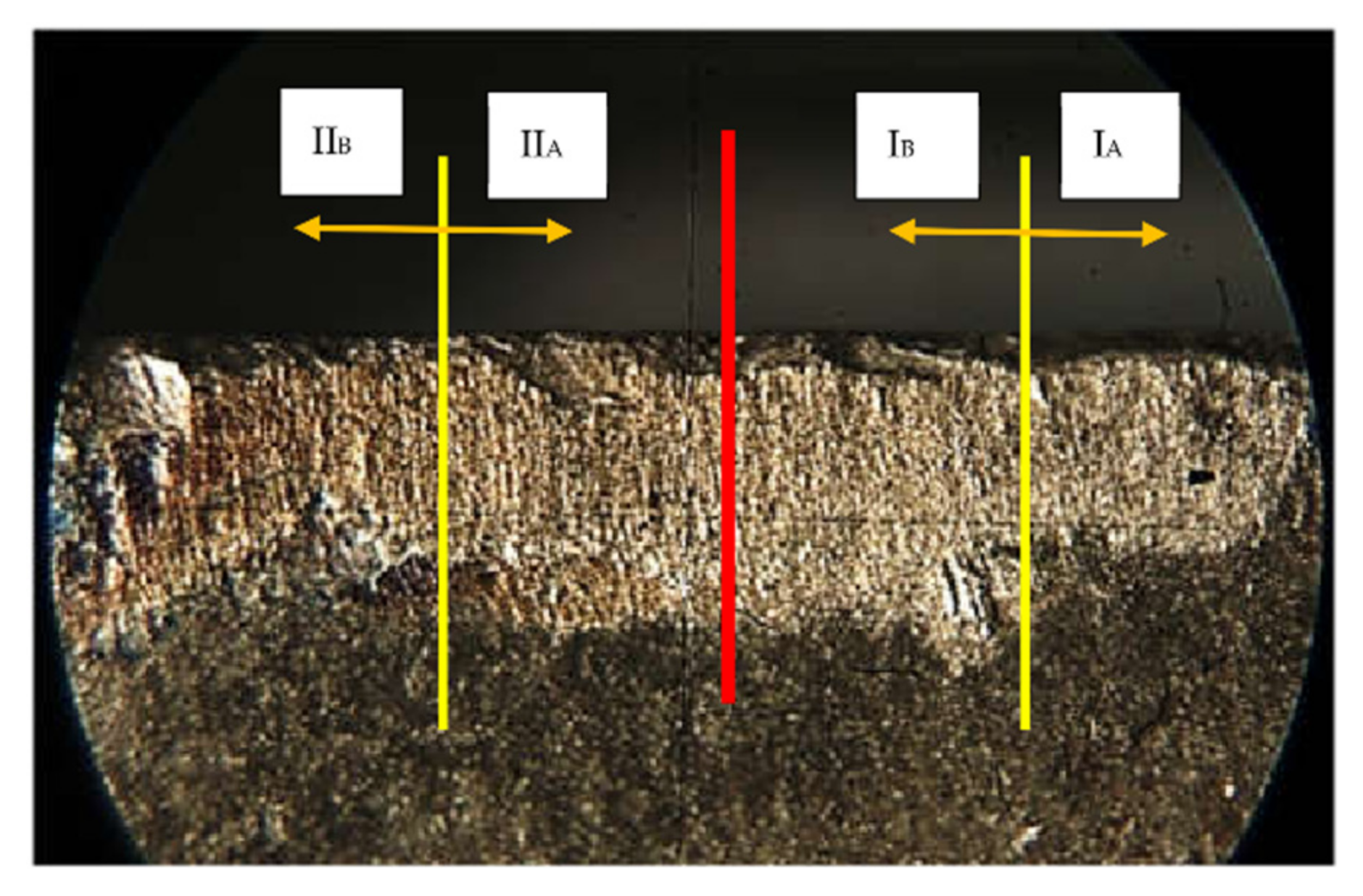
For the edge no. 1 there is a contradiction, namely, the VBMAX/VBB ratio indicates that the wear has a pronounced non-uniform character and the supra-unit ratio between VBB,I and VBB,II shows that the wear is uniform. In order to resolve the contradiction, the symmetry segmentation is applied for the two parts I and II (Figure 19). Using the data in Table 4, Table 7 is obtained.
Based on Table 7, this time, it is clear that part I has a pronounced asymmetric character and the VBMAX/VBB ratio indicates the same thing; consequently, the wear has a pronounced ununiform character.
5. Conclusions
The development of this research lead to the following conclusions:
- This paper, in the state of the art section, presented the actual methods used to assess the wear of cutting tools, centralizing 88 researches and studies over the last decade;
- It highlighted the importance of continuous research in the wear of cutting tools field and also the necessity of a unitary methodology of measurement;
- In this paper is proposed a unitary methodology for measuring wear by microscope so that researchers can obtain comparable values; this methodology can be applied with a level of confidence argued by experimental attempts;
- The development of the proposed methodology requires experimental tries to identify the errors that may occur during the wear measurement; this research also identifies and analyzes the sources of human error in measuring the flank wear;
- The obtained experimental data show the magnitude of the errors that can be made by an operator and also by independent operators when measuring the flank wear;
- The methodology was tested in the case of six worn inserts SPMR150612 type, and from each insert was used one cutting edge for turning C45(1.0503) specimens;
- In a separate section, based on the experimental data, the principles of symmetry were applied and is demonstrated that the wear has a pronounced ununiform character;
- The proposed methodology used to measure the flank wear of the cutting inserts with minimal errors, allows for the collection of results which can be compared between different researchers and can also be easily reproduced.
Author Contributions
Conceptualization, R.D. and G.O.; methodology, R.D. and G.O.; validation, R.D. and G.O.; formal analysis, R.D. and G.O.; investigation, R.D. and G.O.; resources, R.D. and G.O.; data curation, R.D.; writing—original draft preparation, R.D.; writing—review and editing, R.D. and G.O.; supervision, G.O.; project administration, R.D. All authors have read and agreed to the published version of the manuscript.
Funding
This research received no external funding.
Institutional Review Board Statement
Not applicable.
Informed Consent Statement
Not applicable.
Data Availability Statement
Data sharing is not applied.
Conflicts of Interest
The authors declare no conflict of interest.
References
- Siddhpura, A.; Paurobally, R. A review of flank wear prediction methods for tool condition monitoring in a turning process. Int. J. Adv. Manuf. Technol. 2013, 65, 371–393. [Google Scholar] [CrossRef]
- Zhu, D.; Zhang, X.; Ding, H. Tool wear characteristics in machining of nickel-based superalloys. Int. J. Mach. Tools Manuf. 2013, 64, 60–77. [Google Scholar] [CrossRef]
- Xu, C.; Dou, J.; Chai, Y.; Li, H.; Shi, Z.; Xu, J. The relationships between cutting parameters, tool wear, cutting force and vibration. Adv. Mech. Eng. 2018, 10, 1687814017750434. [Google Scholar] [CrossRef]
- International Organization of Standardization. Available online: www.iso.org/standard/9151 (accessed on 1 February 2022).
- Daicu, R.; Dițu, V. Particularities Regarding the Wear of SPMR150612-P30 Metallic Carbide Inserts. Recent J. 2019, 20, 123–128. [Google Scholar] [CrossRef]
- Attanasio, A.; Ceretti, E.; Fiorentino, A.; Cappellini, C.; Giardini, C. Investigation and FEM-based simulation of tool wear in turning operations with uncoated carbide tools. Wear 2010, 269, 344–350. [Google Scholar] [CrossRef]
- Haddag, B.; Nouari, M. Tool wear and heat transfer analyses in dry machining based on multi-steps numerical modelling and experimental validation. Wear 2013, 302, 1158–1170. [Google Scholar] [CrossRef]
- Binder, M.; Klocke, F.; Lung, D. Tool wear simulation of complex shaped coated cutting tools. Wear 2015, 330–331, 600–607. [Google Scholar] [CrossRef]
- Pimenov, D.Y.; Guzeev, V.I. Mathematical model of plowing forces to account for flank wear using FME modeling for orthogonal cutting scheme. Int. J. Adv. Manuf. Technol. 2016, 89, 3149–3159. [Google Scholar] [CrossRef]
- Shi, Z.; Li, X.; Duan, N.; Yang, Q. Evaluation of tool wear and cutting performance considering effects of dynamic nodes movement based on FEM simulation. Chin. J. Aeronaut. 2020, 34, 140–152. [Google Scholar] [CrossRef]
- Dutta, S.; Pal, S.K.; Sen, R. Digital Image Processing in Machining. In Modern Mechanical Engineering. Materials Forming, Machining and Tribology; Davim, J.P., Ed.; Springer: Berlin/Heidelberg, Germany, 2014; Chapter 13; pp. 367–410. [Google Scholar] [CrossRef]
- Wang, W.; Wong, Y.; Hong, G. Flank wear measurement by successive image analysis. Comput. Ind. 2005, 56, 816–830. [Google Scholar] [CrossRef]
- Zhang, C.; Zhang, J. On-line tool wear measurement for ball-end milling cutter based on machine vision. Comput. Ind. 2013, 64, 708–719. [Google Scholar] [CrossRef]
- Li, W.; Singh, H.M.; Guo, Y.B. An online optical system for inspecting tool condition in milling of H13 tool steel and IN 718 alloy. Int. J. Adv. Manuf. Technol. 2012, 67, 1067–1077. [Google Scholar] [CrossRef]
- Zhu, K.; Yu, X. The monitoring of micro milling tool wear conditions by wear area estimation. Mech. Syst. Signal Process. 2017, 93, 80–91. [Google Scholar] [CrossRef]
- Szydłowski, M.; Powalka, B.; Matuszak, M.; Kochmański, P. Machine vision micro-milling tool wear inspection by image reconstruction and light reflectance. Precis. Eng. 2016, 44, 236–244. [Google Scholar] [CrossRef]
- Li, L.; An, Q. An in-depth study of tool wear monitoring technique based on image segmentation and texture analysis. Measurement 2016, 79, 44–52. [Google Scholar] [CrossRef]
- Takaya, Y.; Maruno, K.; Michihata, M.; Mizutani, Y. Measurement of a tool wear profile using confocal fluorescence microscopy of the cutting fluid layer. CIRP Ann. 2016, 65, 467–470. [Google Scholar] [CrossRef]
- Čerče, L.; Pušavec, F.; Kopač, J. 3D cutting tool-wear monitoring in the process. J. Mech. Sci. Technol. 2015, 29, 3885–3895. [Google Scholar] [CrossRef]
- D’Addona, D.M.; Ullah, A.S.; Matarazzo, D. Tool-wear prediction and pattern-recognition using artificial neural network and DNA-based computing. J. Intell. Manuf. 2015, 28, 1285–1301. [Google Scholar] [CrossRef]
- Lipiński, D.; Kacalak, W.; Tomkowski, R. Methodology of evaluation of abrasive tool wear with the use of laser scanning microscopy. Scanning 2013, 36, 53–63. [Google Scholar] [CrossRef]
- Zhang, C.; Yao, X.; Zhang, J.; Jin, H. Tool Condition Monitoring and Remaining Useful Life Prognostic Based on a Wireless Sensor in Dry Milling Operations. Sensors 2016, 16, 795. [Google Scholar] [CrossRef] [Green Version]
- Ghani, J.; Rizal, M.; Nuawi, M.; Ghazali, M.; Haron, C. Monitoring online cutting tool wear using low-cost technique and user-friendly GUI. Wear 2011, 271, 2619–2624. [Google Scholar] [CrossRef]
- Nouri, M.; Fussell, B.K.; Ziniti, B.L.; Linder, E. Real-time tool wear monitoring in milling using a cutting condition independent method. Int. J. Mach. Tools Manuf. 2014, 89, 1–13. [Google Scholar] [CrossRef]
- Singh, D.; Rao, P.V. Flank wear prediction of ceramic tools in hard turning. Int. J. Adv. Manuf. Technol. 2010, 50, 479–493. [Google Scholar] [CrossRef]
- Jozić, S.; Lela, B.; Bajić, D. A New Mathematical Model for Flank Wear Prediction Using Functional Data Analysis Methodology. Adv. Mater. Sci. Eng. 2014, 2014, 138168. [Google Scholar] [CrossRef] [Green Version]
- Denkena, B.; Krüger, M.; Schmidt, J. Condition-based tool management for small batch production. Int. J. Adv. Manuf. Technol. 2014, 74, 471–480. [Google Scholar] [CrossRef]
- Chinchanikar, S.; Choudhury, S.K. Cutting force modeling considering tool wear effect during turning of hardened AISI 4340 alloy steel using multi-layer TiCN/Al2O3/TiN-coated carbide tools. Int. J. Adv. Manuf. Technol. 2015, 83, 1749–1762. [Google Scholar] [CrossRef]
- Jeyakumar, S.; Marimuthu, K.; Ramachandran, T. Prediction of cutting force, tool wear and surface roughness of Al6061/SiC composite for end milling operations using RSM. J. Mech. Sci. Technol. 2013, 27, 2813–2822. [Google Scholar] [CrossRef]
- Wang, G.; Guo, Z.; Qian, L. Tool wear prediction considering uncovered data based on partial least square regression. J. Mech. Sci. Technol. 2014, 28, 317–322. [Google Scholar] [CrossRef]
- Kaya, B.; Oysu, C.; Ertunc, H.M. Force-torque based on-line tool wear estimation system for CNC milling of Inconel 718 using neural networks. Adv. Eng. Softw. 2011, 42, 76–84. [Google Scholar] [CrossRef]
- Rizal, M.; Ghani, J.A.; Nuawi, M.Z.; Haron, C.H.C. Online tool wear prediction system in the turning process using an adaptive neuro-fuzzy inference system. Appl. Soft Comput. 2013, 13, 1960–1968. [Google Scholar] [CrossRef]
- Liu, T.-I.; Song, S.-D.; Liu, G.; Wu, Z. Online monitoring and measurements of tool wear for precision turning of stainless steel parts. Int. J. Adv. Manuf. Technol. 2012, 65, 1397–1407. [Google Scholar] [CrossRef]
- Wang, G.; Cui, Y. On line tool wear monitoring based on auto associative neural network. J. Intell. Manuf. 2012, 24, 1085–1094. [Google Scholar] [CrossRef]
- Gao, D.; Liao, Z.; Lv, Z.; Lu, Y. Multi-scale statistical signal processing of cutting force in cutting tool condition monitoring. Int. J. Adv. Manuf. Technol. 2015, 80, 1843–1853. [Google Scholar] [CrossRef]
- Benkedjouh, T.; Medjaher, K.; Zerhouni, N.; Rechak, S. Health assessment and life prediction of cutting tools based on support vector regression. J. Intell. Manuf. 2015, 26, 213–223. [Google Scholar] [CrossRef] [Green Version]
- Karam, S.; Centobelli, P.; D’Addona, D.M.; Teti, R. Online Prediction of Cutting Tool Life in Turning via Cognitive Decision Making. Procedia CIRP 2016, 41, 927–932. [Google Scholar] [CrossRef]
- Yang, W.-A.; Zhou, W.; Liao, W.; Guo, Y. Prediction of drill flank wear using ensemble of co-evolutionary particle swarm optimization based-selective neural network ensembles. J. Intell. Manuf. 2014, 27, 343–361. [Google Scholar] [CrossRef]
- Fang, N.; Pai, P.S.; Edwards, N. A comparative study of high-speed machining of Ti-6Al-4V and Inconel 718—part II: Effect of dynamic tool edge wear on cutting vibrations. Int. J. Adv. Manuf. Technol. 2013, 68, 1417–1428. [Google Scholar] [CrossRef]
- Fang, N.; Pai, P.S.; Edwards, N. A method of using Hoelder exponents to monitor tool-edge wear in high-speed finish machining. Int. J. Adv. Manuf. Technol. 2014, 72, 1593–1601. [Google Scholar] [CrossRef]
- Postnov, V.V.; Idrisova, Y.V.; Fetsak, S.I. Influence of machine-tool dynamics on the tool wear. Russ. Eng. Res. 2015, 35, 936–940. [Google Scholar] [CrossRef]
- Rao, K.V.; Murthy, B.; Rao, N.M. Cutting tool condition monitoring by analyzing surface roughness, work piece vibration and volume of metal removed for AISI 1040 steel in boring. Measurement 2013, 46, 4075–4084. [Google Scholar] [CrossRef]
- Rmili, W.; Ouahabi, A.; Serra, R.; Leroy, R. An automatic system based on vibratory analysis for cutting tool wear monitoring. Measurement 2016, 77, 117–123. [Google Scholar] [CrossRef]
- Painuli, S.; Elangovan, M.; Sugumaran, V. Tool condition monitoring using K-star algorithm. Expert Syst. Appl. 2014, 41, 2638–2643. [Google Scholar] [CrossRef]
- Aghdam, B.H.; Vahdati, M.; Sadeghi, M.H. Vibration-based estimation of tool major flank wear in a turning process using ARMA models. Int. J. Adv. Manuf. Technol. 2014, 76, 1631–1642. [Google Scholar] [CrossRef]
- Sun, H.; Zhang, X.; Niu, W. In-process cutting tool remaining useful life evaluation based on operational reliability assessment. Int. J. Adv. Manuf. Technol. 2015, 86, 841–851. [Google Scholar] [CrossRef]
- Kilundu, B.; Dehombreux, P.; Chiementin, X. Tool wear monitoring by machine learning techniques and singular spectrum analysis. Mech. Syst. Signal Process. 2011, 25, 400–415. [Google Scholar] [CrossRef]
- Tratar, J.; Pusavec, F.; Kopac, J. Tool wear in terms of vibration effects in milling medium-density fibreboard with an industrial robot. J. Mech. Sci. Technol. 2014, 28, 4421–4429. [Google Scholar] [CrossRef]
- Salonitis, K.; Kolios, A. Reliability assessment of cutting tool life based on surrogate approximation methods. Int. J. Adv. Manuf. Technol. 2014, 71, 1197–1208. [Google Scholar] [CrossRef] [Green Version]
- Bhuiyan, S.; Choudhury, I.; Dahari, M.; Nukman, Y.; Dawal, S. Application of acoustic emission sensor to investigate the frequency of tool wear and plastic deformation in tool condition monitoring. Measurement 2016, 92, 208–217. [Google Scholar] [CrossRef]
- Kulandaivelu, P.; Kumar, P.S.; Sundaram, S. Wear monitoring of single point cutting tool using acoustic emission tech-niques. Sadhana 2013, 38, 211–234. [Google Scholar]
- Zafar, T.; Kamal, K.; Sheikh, Z.; Mathavan, S.; Ali, U.; Hashmi, M.H. A neural network based approach for background noise reduction in airborne acoustic emission of a machining process. J. Mech. Sci. Technol. 2017, 31, 3171–3182. [Google Scholar] [CrossRef]
- Prakash, M.; Kanthababu, M. In-process tool condition monitoring using acoustic emission sensor in microendmilling. Mach. Sci. Technol. 2013, 17, 209–227. [Google Scholar] [CrossRef]
- Bhuiyan, M.S.H.; Choudhury, I.A.; Dahari, M. Monitoring the tool wear, surface roughness and chip formation occurrences using multiple sensors in turning. J. Manuf. Syst. 2014, 33, 476–487. [Google Scholar] [CrossRef]
- Ren, Q.; Baron, L.; Balazinski, M.; Botez, R.; Bigras, P. Tool wear assessment based on type-2 fuzzy uncertainty estimation on acoustic emission. Appl. Soft Comput. 2015, 31, 14–24. [Google Scholar] [CrossRef]
- Li, H.; Wang, Y.; Zhao, P.; Zhang, X.; Zhou, P. Cutting tool operational reliability prediction based on acoustic emission and logistic regression model. J. Intell. Manuf. 2014, 26, 923–931. [Google Scholar] [CrossRef]
- Bombiński, S.; Błażejak, K.; Nejman, M.; Jemielniak, K. Sensor Signal Segmentation for Tool Condition Monitoring. Procedia CIRP 2016, 46, 155–160. [Google Scholar] [CrossRef] [Green Version]
- Balsamo, V.; Caggiano, A.; Jemielniak, K.; Kossakowska, J.; Nejman, M.; Teti, R. Multi Sensor Signal Processing for Catastrophic Tool Failure Detection in Turning. Procedia CIRP 2016, 41, 939–944. [Google Scholar] [CrossRef]
- Cuka, B.; Kim, D.-W. Fuzzy logic based tool condition monitoring for end-milling. Robot. Comput. Manuf. 2017, 47, 22–36. [Google Scholar] [CrossRef]
- Seemuang, N.; McLeay, T.; Slatter, T. Using spindle noise to monitor tool wear in a turning process. Int. J. Adv. Manuf. Technol. 2016, 86, 2781–2790. [Google Scholar] [CrossRef] [Green Version]
- Zhang, K.-F.; Yuan, H.-Q.; Nie, P. A method for tool condition monitoring based on sensor fusion. J. Intell. Manuf. 2015, 26, 1011–1026. [Google Scholar] [CrossRef]
- Khajavi, M.N.; Nasernia, E.; Rostaghi, M. Milling tool wear diagnosis by feed motor current signal using an artificial neural network. J. Mech. Sci. Technol. 2016, 30, 4869–4875. [Google Scholar] [CrossRef]
- Letot, C.; Serra, R.; Dossevi, M.; Dehombreux, P. Cutting tools reliability and residual life prediction from degradation indicators in turning process. Int. J. Adv. Manuf. Technol. 2015, 86, 495–506. [Google Scholar] [CrossRef]
- Liao, Y.; Stephenson, D.A.; Ni, J. A Multifeature Approach to Tool Wear Estimation Using 3D Workpiece Surface Texture Parameters. J. Manuf. Sci. Eng. 2010, 132, 061008. [Google Scholar] [CrossRef]
- Dutta, S.; Kanwat, A.; Pal, S.K.; Sen, R. Correlation study of tool flank wear with machined surface texture in end milling. Measurement 2013, 46, 4249–4260. [Google Scholar] [CrossRef]
- Dutta, S.; Datta, A.; Das Chakladar, N.; Pal, S.; Mukhopadhyay, S.; Sen, R. Detection of tool condition from the turned surface images using an accurate grey level co-occurrence technique. Precis. Eng. 2012, 36, 458–466. [Google Scholar] [CrossRef]
- Dutta, S.; Pal, S.K.; Sen, R. Progressive tool flank wear monitoring by applying discrete wavelet transform on turned surface images. Measurement 2016, 77, 388–401. [Google Scholar] [CrossRef]
- Dutta, S.; Pal, S.K.; Sen, R. On-machine tool prediction of flank wear from machined surface images using texture analyses and support vector regression. Precis. Eng. 2016, 43, 34–42. [Google Scholar] [CrossRef]
- Bhat, N.N.; Dutta, S.; Vashisth, T.; Pal, S.; Pal, S.K.; Sen, R. Tool condition monitoring by SVM classification of machined surface images in turning. Int. J. Adv. Manuf. Technol. 2016, 83, 1487–1502. [Google Scholar] [CrossRef]
- Senthilkumar, N.; Tamizharasan, T. Experimental investigation of cutting zone temperature and flank wear correlation in turning AISI 1045 steel with different tool geometries. Indian J. Eng. Mater. Sci. 2014, 21, 139–148. Available online: http://nopr.niscair.res.in/bitstream/123456789/28780/3/IJEMS%2021(2)%20139-148.pdf (accessed on 6 February 2022).
- Bagavathiappan, S.; Lahiri, B.B.; Suresh, S.; Philip, J.; Jayakumar, T. Online monitoring of cutting tool temperature during micro-end milling using infrared thermography. Insight Non Destr. Test. Cond. Monit. 2015, 57, 9–17. [Google Scholar] [CrossRef]
- Lauro, C.; Brandão, L.; Baldo, D.; Reis, R.; Davim, J.P. Monitoring and processing signal applied in machining processes—A review. Measurement 2014, 58, 73–86. [Google Scholar] [CrossRef]
- Daicu, R.; Oancea, G. Electrical Current at Metal Cutting Process: A Literature Review. Appl. Mech. Mater. 2015, 808, 40–47. [Google Scholar] [CrossRef]
- Medison, V.V. Influence of thermoelectric current on the tool life in cutting titanium alloys. Russ. Eng. Res. 2014, 34, 235–238. [Google Scholar] [CrossRef]
- Ratava, J.; Lohtander, M.; Varis, J. Tool condition monitoring in interrupted cutting with acceleration sensors. Robot. Comput. Manuf. 2017, 47, 70–75. [Google Scholar] [CrossRef]
- Mandal, N.; Mondal, B.; Doloi, B. Application of Back Propagation Neural Network Model for Predicting Flank Wear of Yttria Based Zirconia Toughened Alumina (ZTA) Ceramic Inserts. Trans. Indian Inst. Met. 2015, 68, 783–789. [Google Scholar] [CrossRef]
- DAS, S.R.; Dhupal, D.; Kumar, A. Study of surface roughness and flank wear in hard turning of AISI 4140 steel with coated ceramic inserts. J. Mech. Sci. Technol. 2015, 29, 4329–4340. [Google Scholar] [CrossRef]
- Li, H.; He, G.; Qin, X.; Wang, G.; Lu, C.; Gui, L. Tool wear and hole quality investigation in dry helical milling of Ti-6Al-4V alloy. Int. J. Adv. Manuf. Technol. 2014, 71, 1511–1523. [Google Scholar] [CrossRef]
- Bushlya, V.M.; Gutnichenko, O.A.; Zhou, J.M.; Ståhl, J.-E.; Gunnarsson, S. Tool wear and tool life of PCBN, binderless cBN and wBN-cBN tools in continuous finish hard turning of cold work tool steel. J. Superhard Mater. 2014, 36, 49–60. [Google Scholar] [CrossRef]
- Chinchanikar, S.; Choudhury, S.K. Wear behaviors of single-layer and multi-layer coated carbide inserts in high speed machining of hardened AISI 4340 steel. J. Mech. Sci. Technol. 2013, 27, 1451–1459. [Google Scholar] [CrossRef]
- Valerga, A.; Batista, M.; Bienvenido, R.; Fernández-Vidal, S.; Wendt, C.; Marcos, M. Reverse Engineering Based Methodology for Modelling Cutting Tools. Procedia Eng. 2015, 132, 1144–1151. [Google Scholar] [CrossRef] [Green Version]
- Cabibbo, M.; Forcellese, A.; Raffaeli, R.; Simoncini, M. Reverse Engineering and Scanning Electron Microscopy Applied to the Characterization of Tool Wear in Dry Milling Processes. Procedia CIRP 2017, 62, 233–238. [Google Scholar] [CrossRef]
- Wang, J.; Wang, P.; Gao, R.X. Enhanced particle filter for tool wear prediction. J. Manuf. Syst. 2015, 36, 35–45. [Google Scholar] [CrossRef]
- Hsu, B.-M.; Shu, M.-H.; Wu, L. Dynamic performance modelling and measuring for machine tools with continuous-state wear processes. Int. J. Prod. Res. 2013, 51, 4718–4731. [Google Scholar] [CrossRef]
- Xu, W.; Cao, L. Optimal tool replacement with product quality deterioration and random tool failure. Int. J. Prod. Res. 2014, 53, 1736–1745. [Google Scholar] [CrossRef]
- Salimiasl, A.; Özdemir, A. Analyzing the performance of artificial neural network (ANN)-, fuzzy logic (FL)-, and least square (LS)-based models for online tool condition monitoring. Int. J. Adv. Manuf. Technol. 2016, 87, 1145–1158. [Google Scholar] [CrossRef]
- Yang, W.-A.; Zhou, Q.; Tsui, K.-L. Differential evolution-based feature selection and parameter optimisation for extreme learning machine in tool wear estimation. Int. J. Prod. Res. 2015, 54, 4703–4721. [Google Scholar] [CrossRef]
- Jafarian, F.; Taghipour, M.; Amirabadi, H. Application of artificial neural network and optimization algorithms for optimizing surface roughness, tool life and cutting forces in turning operation. J. Mech. Sci. Technol. 2013, 27, 1469–1477. [Google Scholar] [CrossRef]
- Ostasevicius, V.; Jurenas, V.; Augutis, V.; Gaidys, R.; Cesnavicius, R.; Kizauskiene, L.; Dundulis, R. Monitoring the condition of the cutting tool using self-powering wireless sensor technologies. Int. J. Adv. Manuf. Technol. 2016, 88, 2803–2817. [Google Scholar] [CrossRef] [Green Version]
- European Steel and Alloy Grades/Numbers. Available online: http://www.steelnumber.com/en/steel_composition_eu.php?name_id=152 (accessed on 1 February 2022).
- Microscope International. Available online: https://microscopeinternational.com/mitutoyo-vision-unit-10d-system-retrofit-microscopes-export/ (accessed on 6 February 2022).
- Shop Mitutoyo. Available online: https://shop.mitutoyo.ro/web/mitutoyo/en_RO/mitutoyo/01.02.07.01/Digital%20Micrometer%20Head/$catalogue/mitutoyoData/PR/164-163/index.xhtml (accessed on 6 February 2022).
- Mitutoyo. Available online: https://www.mitutoyo.se/application/files/8315/5888/7807/PRE13034_Measuring_Microscopes_SMALL.pdf (accessed on 6 February 2022).
- Daicu, R. Innovative Approaches to Metal Cutting. Ph.D. Thesis, Transilvania University of Brasov, Brasov, Romania, July 2021. [Google Scholar]
- Hirox. Available online: https://www.hirox.com/catalog/pdf/cat_RH-2000_en2_A.pdf (accessed on 6 February 2022).
Figure 1.
Main causes for wear appearance.

Figure 2.
Flank wear, according to reference [4].
Figure 2.
Flank wear, according to reference [4].
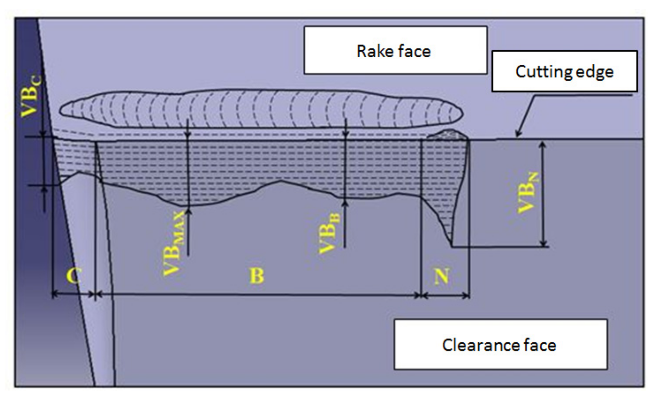
Figure 3.
Crater wear, according to reference [4].
Figure 3.
Crater wear, according to reference [4].
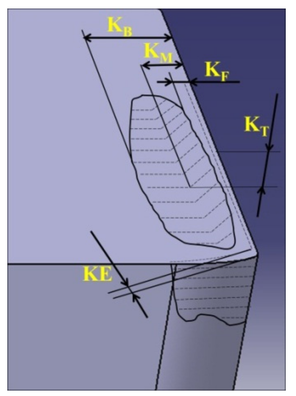
Figure 4.
Cutting tool wear measurement methods.
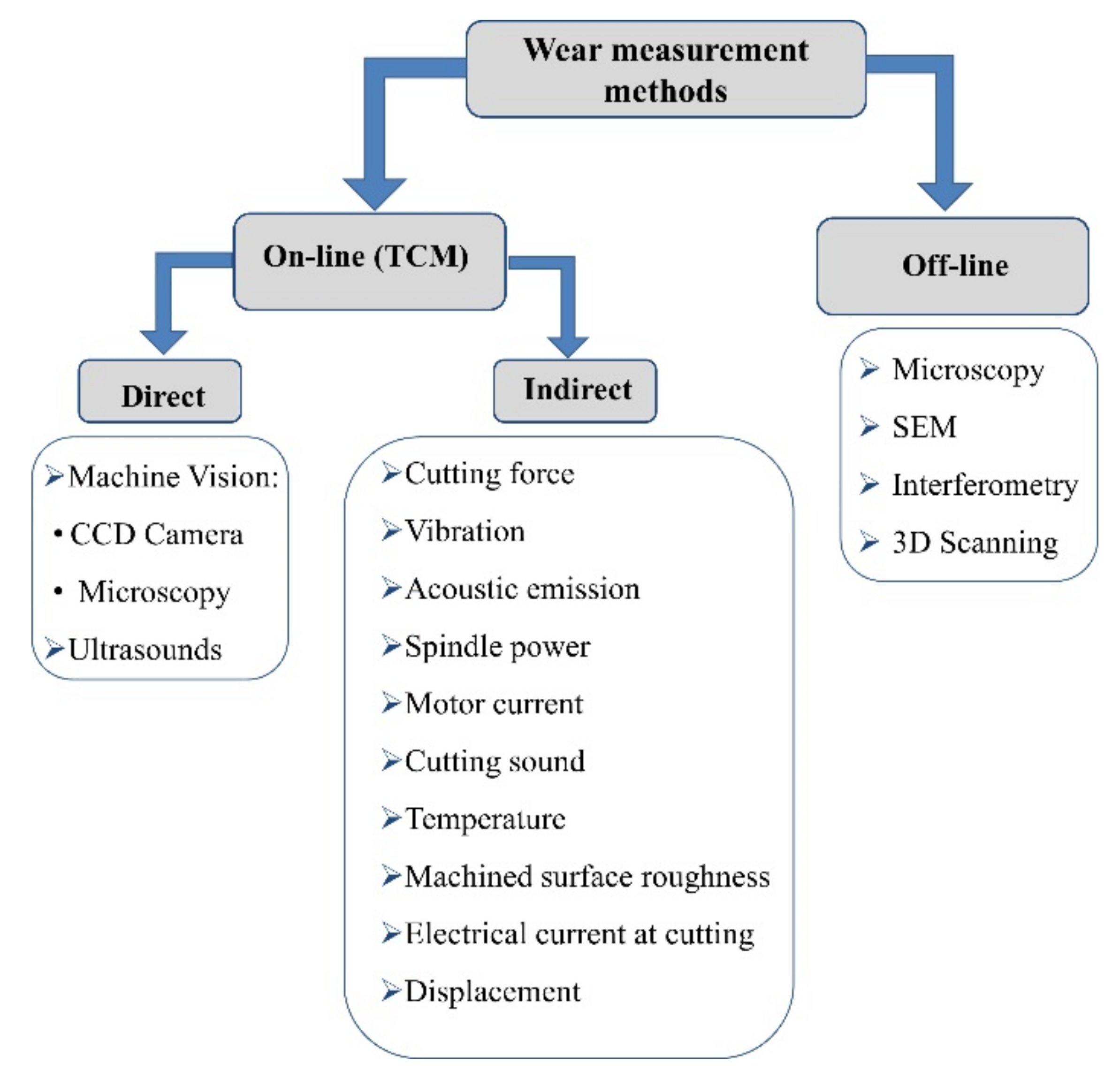

Figure 6.
Microscope for measuring the cutting insert wear [5].
Figure 6.
Microscope for measuring the cutting insert wear [5].
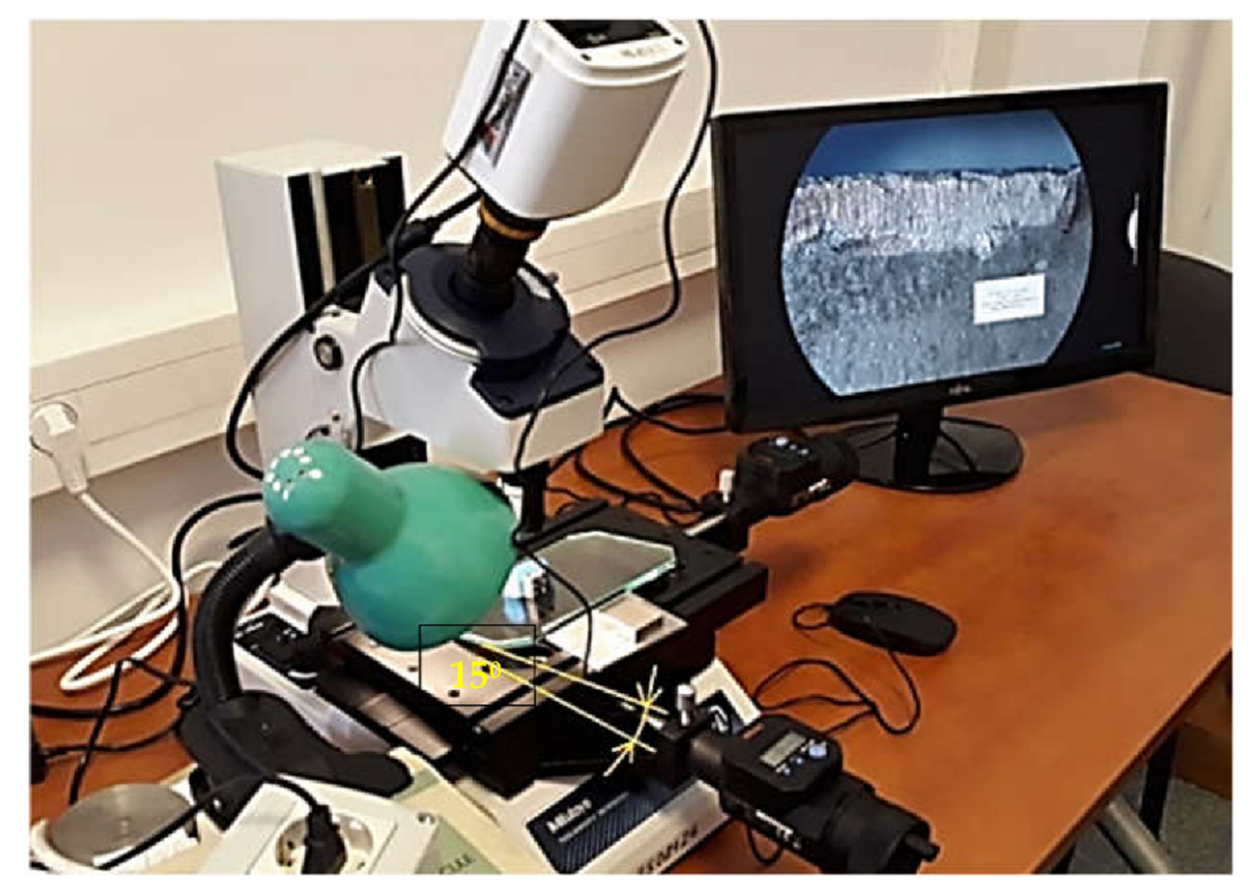
Figure 7.
Wear of cutting insert 1 [5].
Figure 7.
Wear of cutting insert 1 [5].

Figure 8.
Wear of cutting insert 2 [5].
Figure 8.
Wear of cutting insert 2 [5].
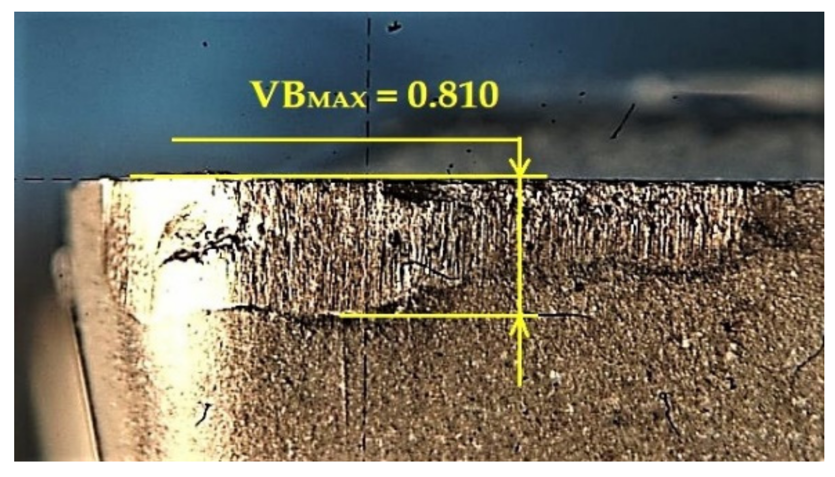
Figure 9.
Wear of cutting insert 3 [5].
Figure 9.
Wear of cutting insert 3 [5].
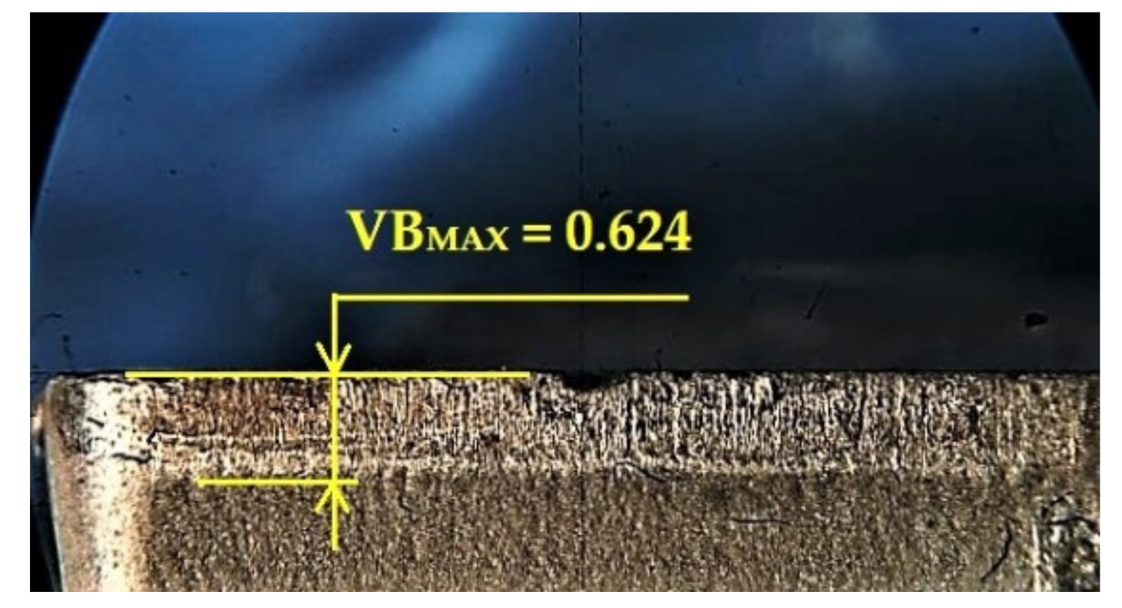
Figure 10.
Wear of cutting insert 4 [5].
Figure 10.
Wear of cutting insert 4 [5].
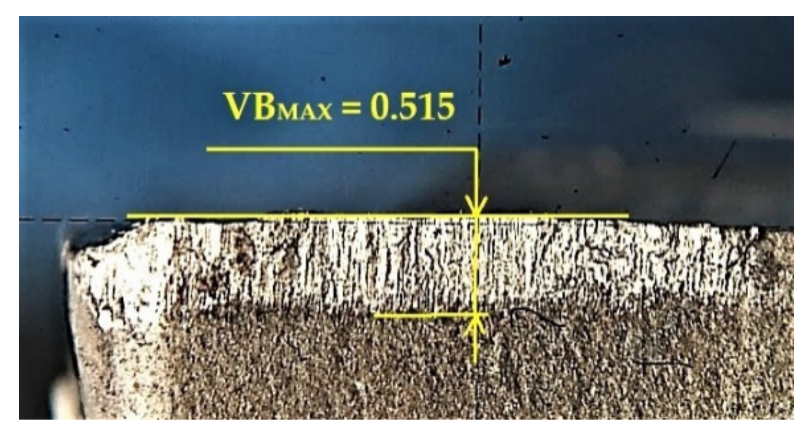
Figure 11.
Wear of cutting insert 5 [5].
Figure 11.
Wear of cutting insert 5 [5].
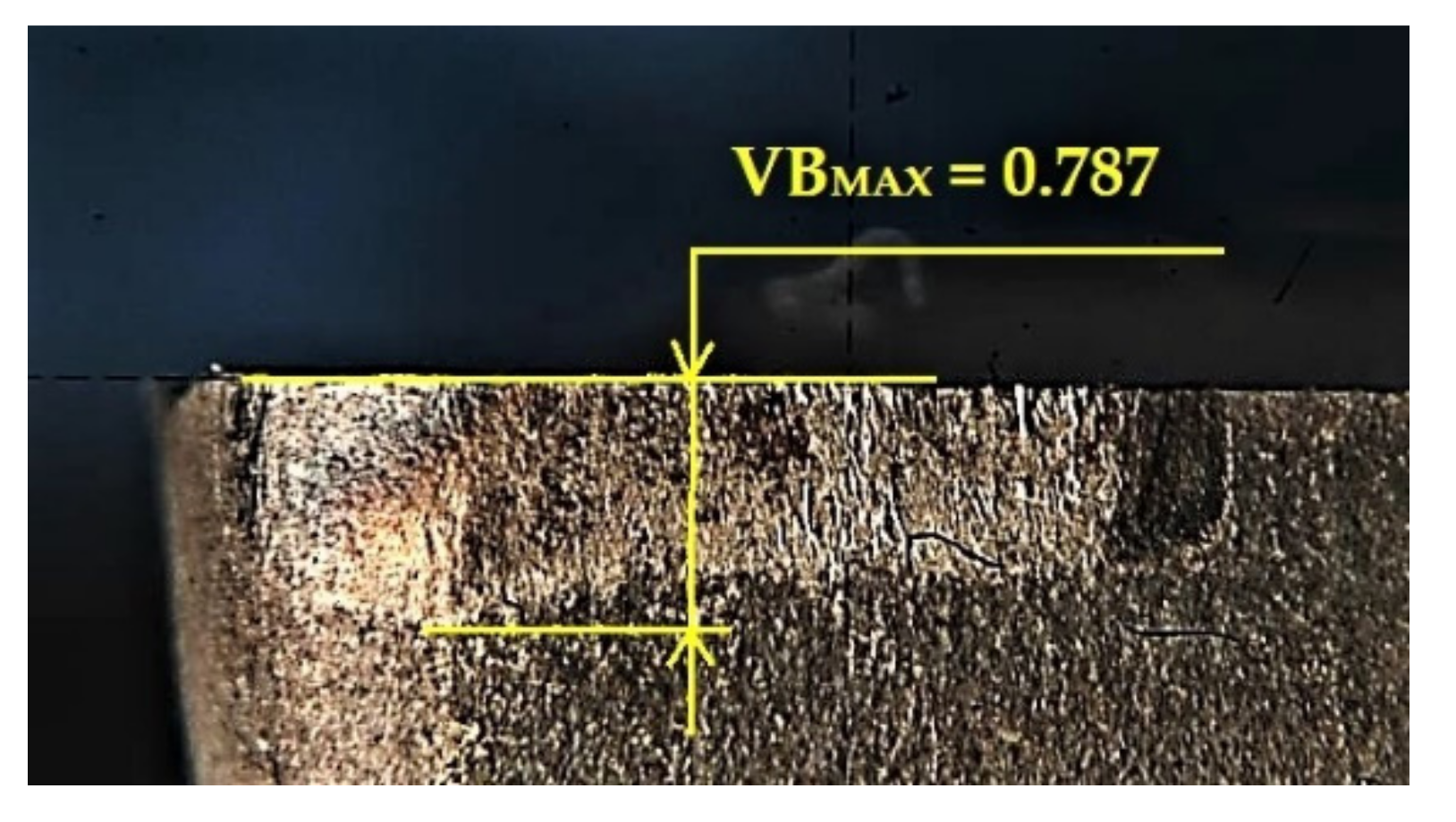
Figure 12.
Wear of cutting insert 6 [5].
Figure 12.
Wear of cutting insert 6 [5].

Figure 13.
Determination of the rectilinear worn edge length [94].
Figure 13.
Determination of the rectilinear worn edge length [94].
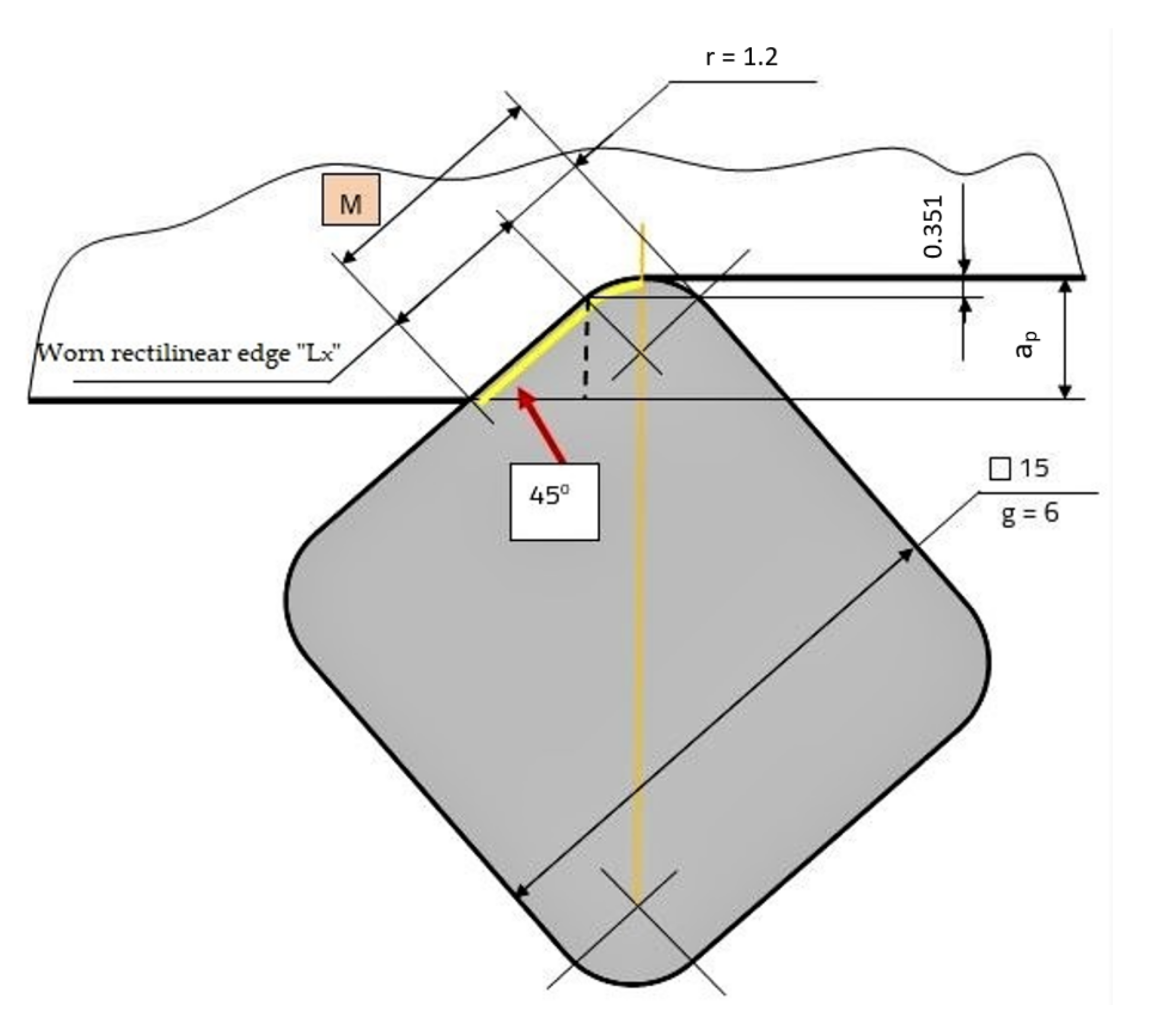
Figure 14.
Sources of human error in measuring wear [91].
Figure 14.
Sources of human error in measuring wear [91].
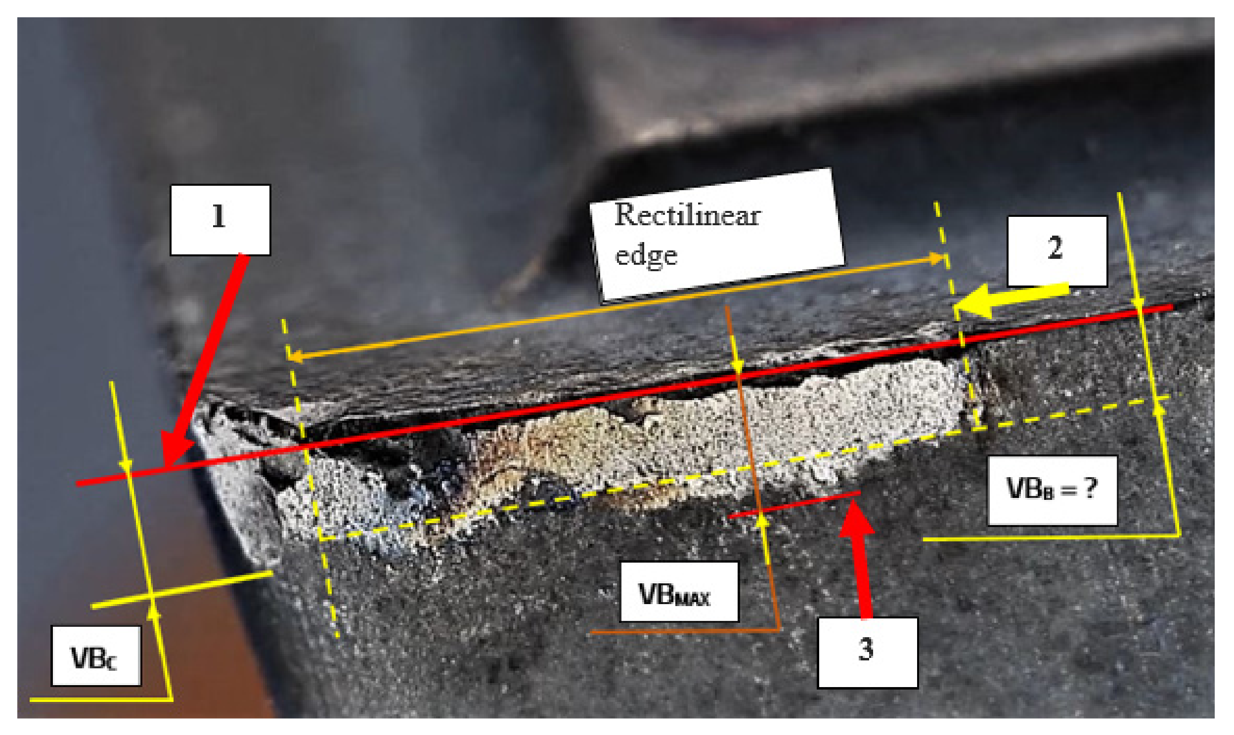
Figure 15.
Maximum difference for measurements repeated 12 times by a single operator [94].
Figure 15.
Maximum difference for measurements repeated 12 times by a single operator [94].
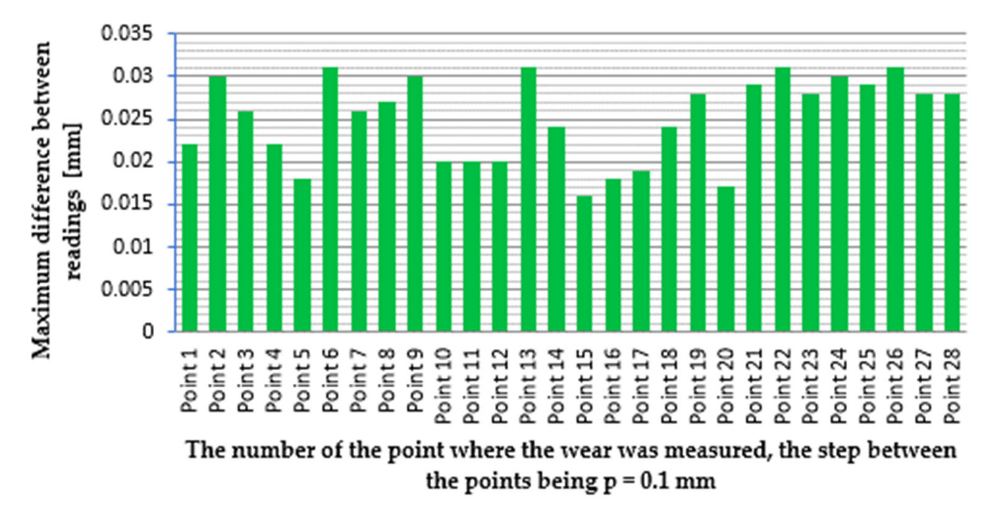
Figure 16.
Average wear value for 12 measurements [94].
Figure 16.
Average wear value for 12 measurements [94].
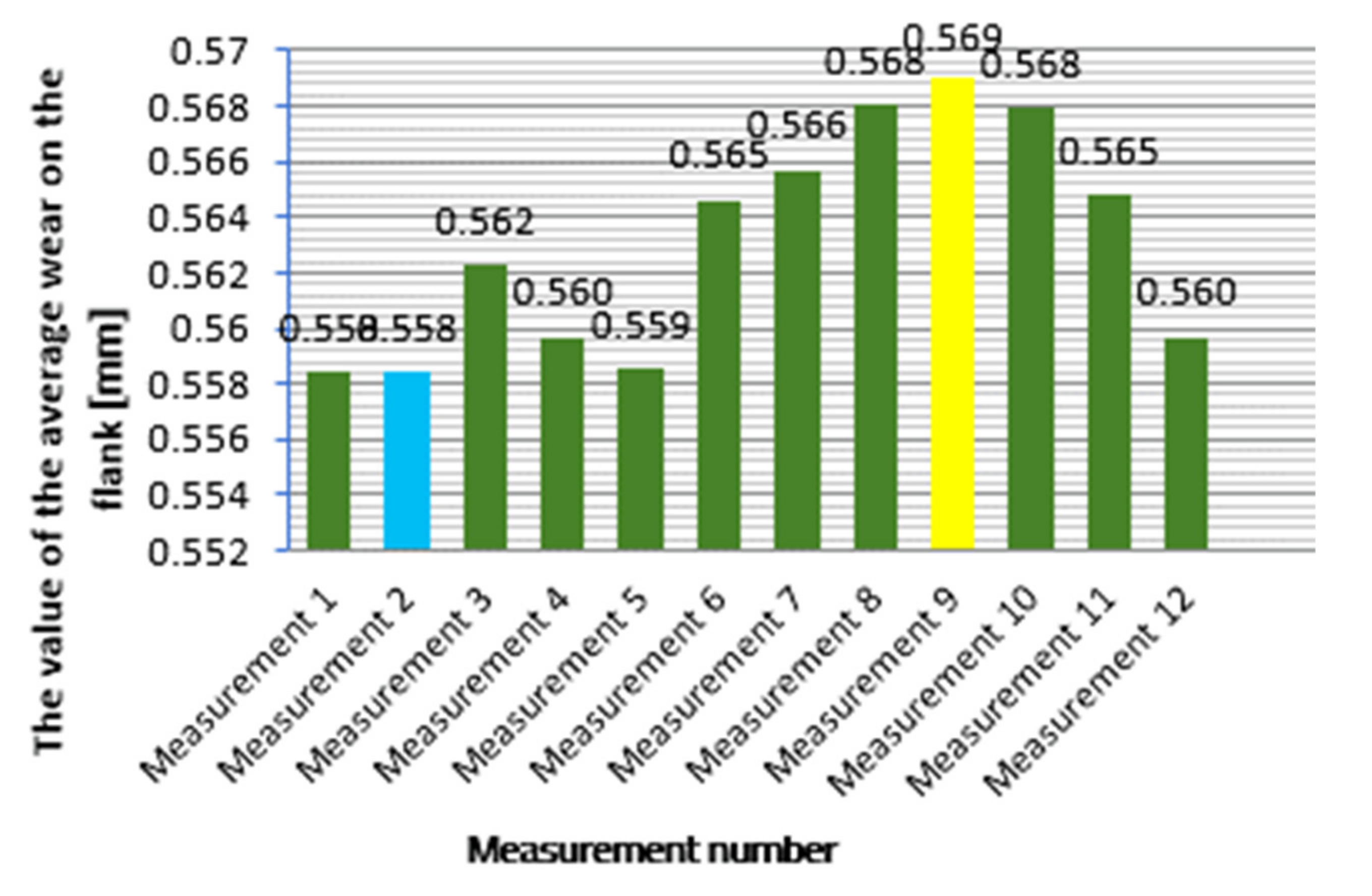
Figure 17.
Maximum difference for the measured wear values by independent operators [94].
Figure 17.
Maximum difference for the measured wear values by independent operators [94].
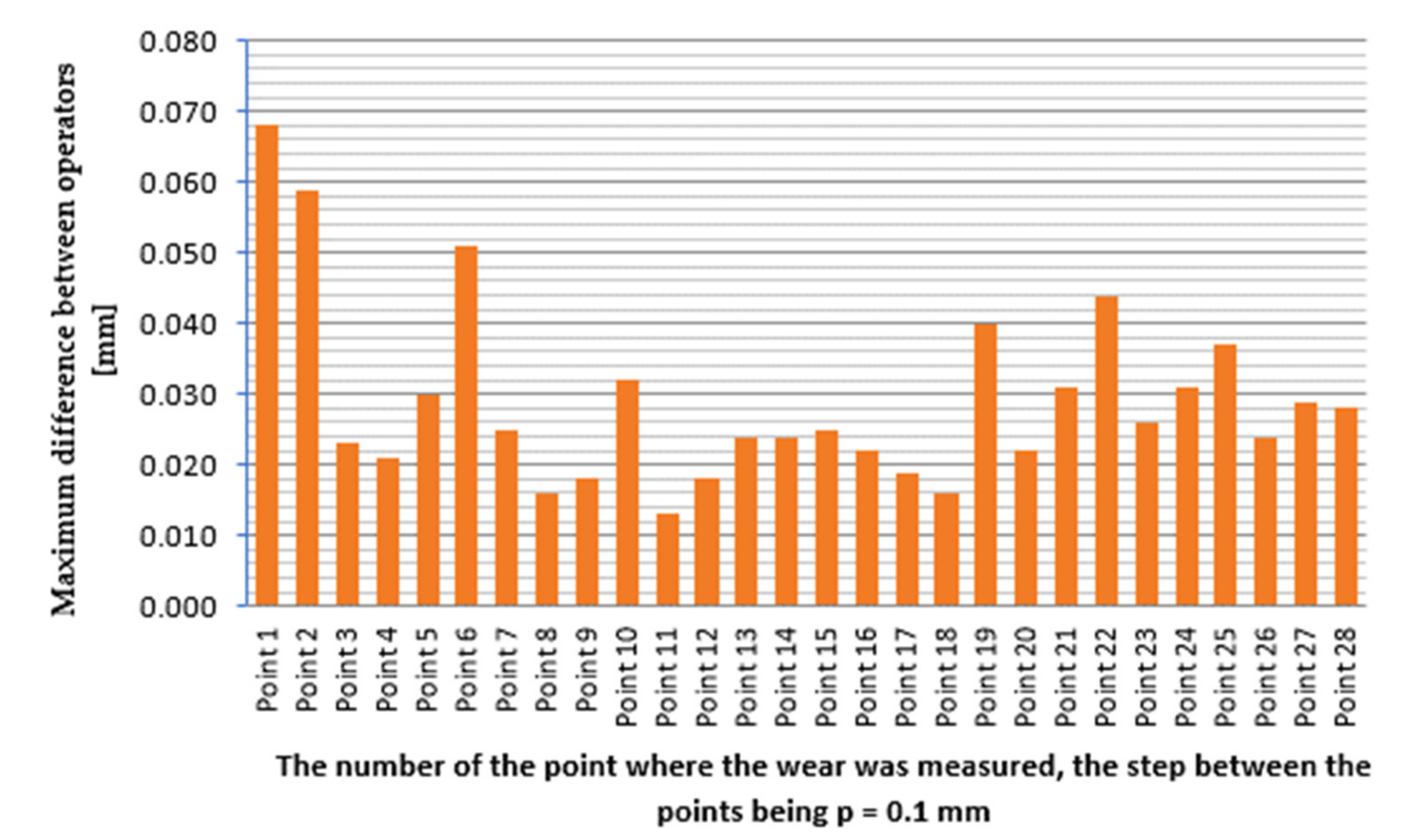
Figure 18.
Applying symmetry principle to characterize the wear.
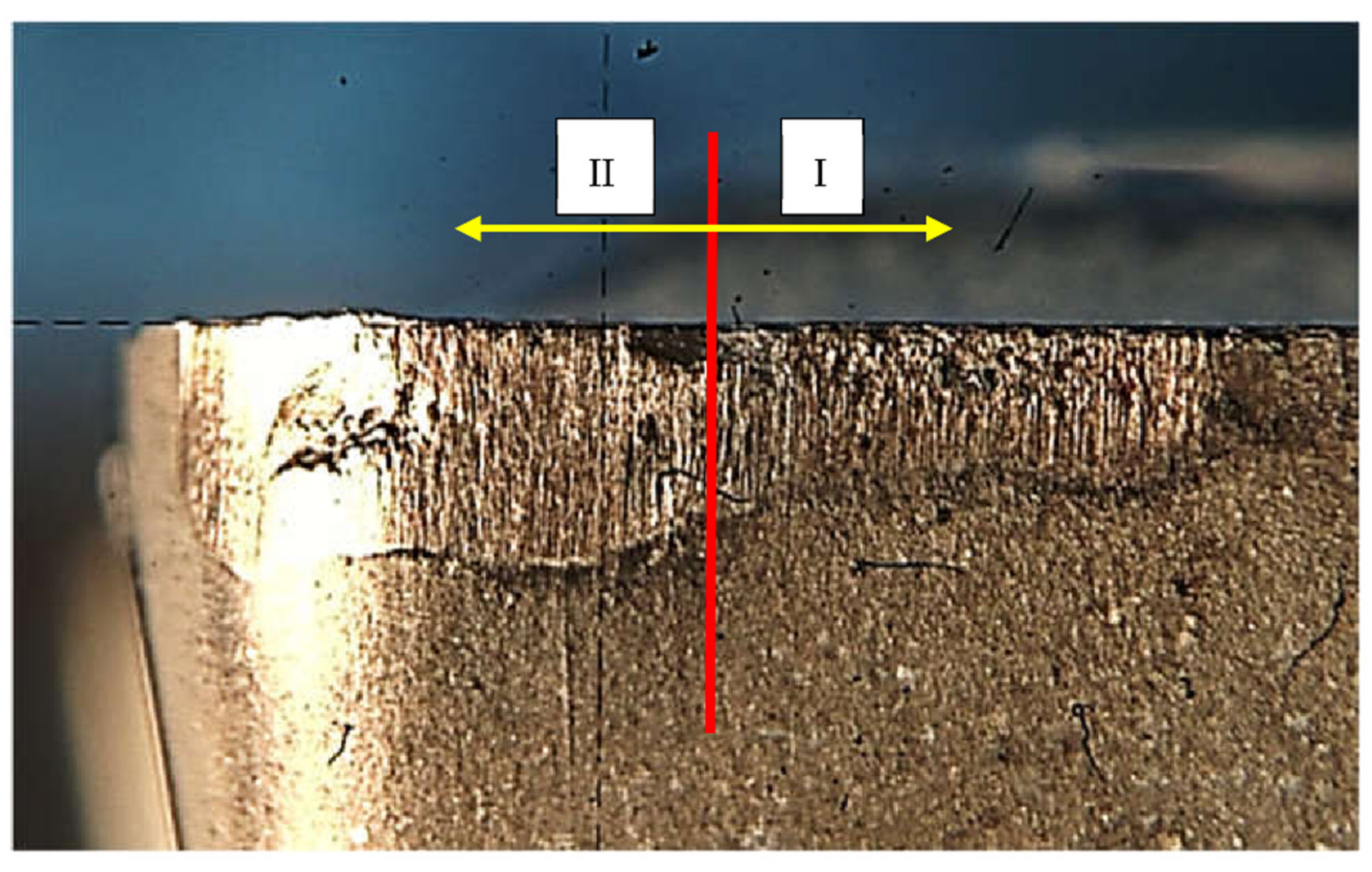
Figure 19.
Symmetry segmentation when characterizing wear for edge no. 1.

Table 1.
Cutting parameters used for turning [5].
Table 1.
Cutting parameters used for turning [5].
| Cutting Parameters No. Cutting Fluids | Cutting Insert 1 | Cutting Insert 2 | Cutting Insert 3 | Cutting Insert 4 | Cutting Insert 5 | Cutting Insert 6 |
|---|---|---|---|---|---|---|
| Cutting speed [m/min] | 106 | 106 | 106 | 106 | 106 | 106 |
| Feed rate [mm/rev] | 0.208 | 0.208 | 0.208 | 0.208 | 0.208 | 0.208 |
| Depth-of-cut [mm] | 2.25 | 2.5 | 4.4 | 3 | 2 | 2.5 |
Table 2.
Values of repeated positioning of the horizontal reticle of the 2D microscope on the edge of the cutting insert [94].
Table 2.
Values of repeated positioning of the horizontal reticle of the 2D microscope on the edge of the cutting insert [94].
| Repetition No. | Deviation from the First Positioning (mm) | Repetition No. | Deviation from the First Positioning (mm) | Repetition No. | Deviation from the First Positioning (mm) |
|---|---|---|---|---|---|
| 1 | 0.002 | 8 | −0.002 | 15 | −0.003 |
| 2 | 0.001 | 9 | 0.001 | 16 | −0.002 |
| 3 | 0.000 | 10 | 0.001 | 17 | 0.000 |
| 4 | 0.002 | 11 | −0.001 | 18 | 0.000 |
| 5 | 0.002 | 12 | 0.001 | 19 | 0.001 |
| 6 | −0.001 | 13 | 0.000 | 20 | −0.001 |
| 7 | 0.000 | 14 | 0.000 | ||
| Maximum difference from the first positioning | 0.003 | ||||
| The average difference from the first positioning | 0.0005 | ||||
| Maximum difference | 0.005 | ||||
Table 3.
Values of repeated positioning of the vertical reticle of the 2D microscope on the edge of the cutting insert [94].
Table 3.
Values of repeated positioning of the vertical reticle of the 2D microscope on the edge of the cutting insert [94].
| Repetition No. | Deviation from the First Positioning (mm) | Repetition No. | Deviation from the First Positioning (mm) | Repetition No. | Deviation from the First Positioning (mm) |
|---|---|---|---|---|---|
| 1 | −0.002 | 8 | −0.003 | 15 | 0.000 |
| 2 | −0.001 | 9 | −0.004 | 16 | 0.002 |
| 3 | 0.002 | 10 | −0.003 | 17 | 0.001 |
| 4 | −0.003 | 11 | 0.000 | 18 | −0.003 |
| 5 | 0.000 | 12 | 0.000 | 19 | 0.002 |
| 6 | −0.001 | 13 | 0.000 | 20 | 0.001 |
| 7 | −0.001 | 14 | 0.001 | ||
| Maximum difference from the first positioning | 0.004 | ||||
| The average difference from the first positioning | 0.0006 | ||||
| Maximum difference | 0.006 | ||||
Table 4.
Measured wear values [94].
Table 4.
Measured wear values [94].
| Edge No. | The No. of Points for Measuring the Wear | Wear Values VBB [mm] |
|---|---|---|
| 1 | 28 | 0.372; 0.450; 0.459; 0.472; 0.458; 0.483; 0.559; 0.652; 0.686; 0.595; 0.596; 0.608; 0.624; 0.599; 0.598; 0.604; 0.619; 0.593; 0.563; 0.570; 0.543; 0.458; 0.451; 0.499; 0.585; 0.643; 0.643; 0.654 |
| 2 | 31 | 0.110; 0.247; 0.467; 0.512; 0.536; 0.527; 0.530; 0.483; 0.465; 0.477; 0.493; 0.504; 0.502; 0.489; 0.511; 0.546; 0.584; 0.626; 0.640; 0.685; 0.708; 0.746; 0.797; 0.805; 0.804; 0.810; 0.779; 0.756; 0.747; 0.753; 0.764 |
| 3 | 58 | 0.423; 0.492; 0.494; 0.481; 0.521; 0.555; 0.545; 0.548; 0.550; 0.553; 0.567; 0.574; 0.533; 0.541; 0.547; 0.529; 0.534; 0.553; 0.555; 0.530; 0.542; 0.539; 0.536; 0.538; 0.517; 0.504; 0.515; 0.520; 0.514; 0.537; 0.541; 0.518; 0.538; 0.558; 0.547; 0.563; 0.546; 0.558; 0.545; 0.537; 0.560; 0.576; 0.562; 0.548; 0.563; 0.541; 0.560; 0.578; 0.562; 0.571; 0.582; 0.597; 0.624; 0.588; 0.579; 0.578; 0.594; 0.596 |
| 4 | 38 | 0.424; 0.433; 0.464; 0.434; 0.455; 0.401; 0.397; 0.406; 0.456; 0.472; 0.501; 0.454; 0.440; 0.447; 0.445; 0.466; 0.482; 0.455; 0.469; 0.478; 0.477; 0.474; 0.482; 0.515; 0.504; 0.478; 0.502; 0.468; 0.471; 0.467; 0.470; 0.438; 0.478; 0.503; 0.484; 0.582; 0.598; 0.578 |
| 5 | 25 | 0.424; 0.518; 0.545; 0.586; 0.612; 0.606; 0.616; 0.631; 0.622; 0.645; 0.662; 0.631; 0.654; 0.701; 0.665; 0.664; 0.695; 0.740; 0.757; 0.745; 0.733; 0.722; 0.749; 0.787; 0.782 |
| 6 | 31 | 0.591; 0.608; 0.634; 0.626; 0.609; 0.628; 0.673; 0.676; 0.713; 0.690; 0.661; 0.637; 0.641; 0.649; 0.639; 0.652; 0.650; 0.638; 0.662; 0.647; 0.685; 0.658; 0.654; 0.650; 0.664; 0.611; 0.613; 0.592; 0.610; 0.639; 0.443 |
Table 5.
Average wear, maximum wear and VBMAX/VBB ratio [94].
Table 5.
Average wear, maximum wear and VBMAX/VBB ratio [94].
| Edge No. | The No. of Points for Measuring the Wear | Average Wear VBB (mm) | Maximum Wear VBMAX (mm) | VBMAX/VBB |
|---|---|---|---|---|
| 1 | 28 | 0.558 | 0.686 | 1.229 |
| 2 | 31 | 0.647 | 0.810 | 1.252 |
| 3 | 58 | 0.547 | 0.624 | 1.141 |
| 4 | 38 | 0.463 | 0.515 | 1.112 |
| 5 | 25 | 0.660 | 0.787 | 1.192 |
| 6 | 31 | 0.637 | 0.713 | 1.119 |
Table 6.
Average and maximum wear, VBMAX/VBB, average wear I and II, superunit ratio between VBB,I and VBB,II.
Table 6.
Average and maximum wear, VBMAX/VBB, average wear I and II, superunit ratio between VBB,I and VBB,II.
| Edge No. | The No. of Points for Measuring the Wear | Average Wear VBB (mm) | Maximum Wear VBMAX (mm) | VBMAX/VBB | VBB,I (mm) | VBB,II (mm) | Superunit Ratio between VBB,I and VBB,II |
|---|---|---|---|---|---|---|---|
| 1 | 28 | 0.558 | 0.686 | 1.229 | 0.544 | 0.574 | 1.055 |
| 2 | 31 | 0.647 | 0.810 | 1.252 | 0.462 | 0.734 | 1.589 |
| 3 | 58 | 0.547 | 0.624 | 1.141 | 0.529 | 0.564 | 1.066 |
| 4 | 38 | 0.463 | 0.515 | 1.112 | 0.447 | 0.497 | 1.112 |
| 5 | 25 | 0.660 | 0.787 | 1.192 | 0.596 | 0.728 | 1.221 |
| 6 | 31 | 0.637 | 0.713 | 1.119 | 0.645 | 0.628 | 1.027 |
Table 7.
Average and maximum wear, VBMAX/VBB, average wear A, average wear B, and superunit ratio between VBB,A and VBB,B.
Table 7.
Average and maximum wear, VBMAX/VBB, average wear A, average wear B, and superunit ratio between VBB,A and VBB,B.
| Edge No. | The No. of Points for Measuring the Wear | Average Wear VBB (mm) | Maximum Wear VBMAX (mm) | VBMAX/VBB | VBB,A (mm) | VBB,B (mm) | Superunit Ratio between VBB,A and VBB,B |
|---|---|---|---|---|---|---|---|
| I | 14 | 0.544 | 0.686 | 1.261 | 0.465 | 0.623 | 1.340 |
| II | 14 | 0.573 | 0.654 | 1.141 | 0.584 | 0.562 | 1.039 |
Publisher’s Note: MDPI stays neutral with regard to jurisdictional claims in published maps and institutional affiliations. |
© 2022 by the authors. Licensee MDPI, Basel, Switzerland. This article is an open access article distributed under the terms and conditions of the Creative Commons Attribution (CC BY) license (https://creativecommons.org/licenses/by/4.0/).
Share and Cite
MDPI and ACS Style
Daicu, R.; Oancea, G. Methodology for Measuring the Cutting Inserts Wear. Symmetry 2022, 14, 469. https://doi.org/10.3390/sym14030469
AMA Style
Daicu R, Oancea G. Methodology for Measuring the Cutting Inserts Wear. Symmetry. 2022; 14(3):469. https://doi.org/10.3390/sym14030469
Chicago/Turabian StyleDaicu, Raluca, and Gheorghe Oancea. 2022. "Methodology for Measuring the Cutting Inserts Wear" Symmetry 14, no. 3: 469. https://doi.org/10.3390/sym14030469
Note that from the first issue of 2016, this journal uses article numbers instead of page numbers. See further details here.